IFIC/16-34
Lepton number violation in 331 models

Abstract

Different models based on the extended $SU(3)_{C}\times SU(3)_{L}\times U(1)_{X}$ (331) gauge group have been proposed over the past four decades. Yet, despite being an active research topic, the status of lepton number in 331 models has not been fully addressed in the literature, and furthermore many of the original proposals can not explain the observed neutrino masses. In this paper we review the basic features of various 331 models, focusing on potential sources of lepton number violation. We then describe different modifications which can be made to the original models in order to accommodate neutrino (and charged lepton) masses.

March 15, 2024

Keywords: 331 models, extended gauge groups, neutrino mass, lepton number.

1 Introduction

It is conceivable that the Standard Model gauge symmetry $SU(3)_{C}\times SU(2)_{L}\times U(1)_{Y}$ (321) is just a remnant of a larger one. Indeed, such scenarios are attractive as they are able to unify the three gauge couplings, provided that the extended gauge group is simple [1, 2, 3, 4]. However, one should not exclude the possibility that the enlarged group is a product of simple factors. This could happen as an intermediate step towards a grand unified group. A famous example is the left-right symmetric group $SU(3)_{C}\times SU(2)_{L}\times SU(2)_{R}\times U(1)_{B-L}$ [5, 6, 7], which fits neatly into $SO(10)$. Another possibility is $SU(3)_{C}\times SU(3)_{L}$, yet with such models one cannot get the correct fermion masses [8]. On the other hand, it was realized long ago [9, 10, 11] that with an extra $U(1)_{X}$ it is possible to construct viable models.

These $SU(3)_{C}\times SU(3)_{L}\times U(1)_{X}$ (331) models have received considerable attention in connection with various topics: neutrino mass generation [12, 13, 14, 15, 16, 17, 18, 19, 20, 21, 22, 23, 24, 25, 26, 27, 28, 29, 30, 31], flavour symmetries [32, 33, 34, 35, 36, 37, 38, 39, 40, 41, 42, 43], quark flavour observables [44, 45, 46, 47, 48, 49, 50, 51] or the recent LHC diphoton excess [52, 53, 54, 55, 56, 57], among others. Underpinning this interest is the fact that the 331 to 321 symmetry breaking energy scale can be of the TeV order, hence it could possibly be explored at the LHC; see for example [58, 59, 60, 61, 62, 63, 64, 65].

However, despite the large list of papers on 331 models, the issue of lepton number violation (LNV) has not been fully addressed in the literature and, in fact, many misleading statements on the subject can be found in papers on 331 models. It turns out that models based on this extended symmetry can be quite different from one another since the way the 321 group is embedded in the 331 group is not unique. In particular (a) the existence of neutrino masses, (b) the nature of neutrinos and (c) the status of lepton number varies markedly among 331 models. As such, with this work we intend to collect and summarize the relevant information concerning lepton number and neutrino mass generation in this class of models.

We have found that several of the originally proposed 331 models can not explain correctly the observed neutrino masses (nor charged lepton masses, in one case). Thus, it is necessary to extend these models and we present several possible modifications that can bring these models in agreement with experimental data, some of which have already been considered before [66, 67, 68, 69, 70, 14]. We focus here (mostly) on neutrino masses and mixings and leave aside other LNV processes, which we mention only briefly when it is relevant.

The rest of this paper is organized as follows. Section 2 describes the basic features of six different 331 models. Four of these fall into a particular subclass since they have a common structure (they all follow what we call the SVS framework, after its prototype model [9]). To cover the full variety of 331 models, we then discuss two more models, which do not follow the SVS scheme, and clarify LNV related issues in them as well. None of the basic models in the SVS class generates lepton masses and mixings in a fully satisfactory way, hence modifications are required. A list of simple improvements is discussed in section 3. For each of the possibilities in our list we give a brief description on how the modified versions of the original models can be brought into agreement with experimental neutrino (and charged lepton) data. Finally, in section 4 we summarize the most important points in this manuscript. An appendix at the end of the text provides supplementary information.

2 The $SU(3)_{L}\times U(1)_{X}$ group and basic 331 models

One can build different 331 models, not just by changing the field content, but also by varying the way in which the SM electroweak gauge group is embedded in $SU(3)_{L}\times U(1)_{X}$. This can be encoded in a continuous parameter $\beta$ which controls the relation between the hypercharge $Y$, $X$, and the $T_{8}$ generator of $SU(3)_{L}$:

$$Y =\beta T_{8}+X\,.$$ (1)

From here one can derive that $SU(3)_{L}\times U(1)_{X}$ representations break as follows into $SU(2)_{L}\times U(1)_{Y}$ representations (more details can be found in the appendix):

$$\left(\mathbf{3},x\right) \rightarrow\left(\widehat{\mathbf{2}},x+\frac{1}{2\sqrt{3}}\beta\right)+\left(\widehat{\mathbf{1}},x-\frac{1}{\sqrt{3}}\beta\right)\,,$$ (2)

$$\left(\overline{\mathbf{6}},x\right) \rightarrow\left(\widehat{\mathbf{3}},x-\frac{1}{\sqrt{3}}\beta\right)+\left(\widehat{\mathbf{2}},x+\frac{1}{2\sqrt{3}}\beta\right)+\left(\widehat{\mathbf{1}},x+\frac{2}{\sqrt{3}}\beta\right)\,,$$ (3)

$$\left(\mathbf{8},0\right) \rightarrow\left(\widehat{\mathbf{3}},0\right)+\left(\widehat{\mathbf{1}},0\right)+\left(\widehat{\mathbf{2}},-\frac{\sqrt{3}}{2}\beta\right)+\left(\widehat{\mathbf{2}},\frac{\sqrt{3}}{2}\beta\right)\,.$$ (4)

Together with the requirement $\left|\beta\right|<\tan^{-1}\theta_{W}\approx 1.8$ (obtainable from equation (143) and the fact that $g^{2}_{X}$ must be positive), these equations show that there are only four values of $\beta$ for which it is possible to avoid colorless, fractionally charged fermions. Bearing this constraint in mind, we can then describe six different 331 models:

• In the first four models, the three lepton families are in equal representations, but the quarks are not. The structure of these models is similar, with the main difference between them being the value of $\beta$: $-1/\sqrt{3}$ in the Singer-Valle-Schechter (SVS) model [9], $-\sqrt{3}$ in the Pisano-Pleitez-Frampton (PPF) model [10, 11], $1/\sqrt{3}$ in the Pleitez-Özer model [71, 72], and $\sqrt{3}$ in what we call the model X. They all share a common structure, which we call the SVS framework below.

• The flipped model [73], where quark families are all in the same representations, but leptons are not.

• The $E_{6}$ model [74], where complete family replication is true for both the lepton and quark sectors.

2.1 The Singer-Valle-Schechter (SVS) model

The first 331 model with three generations of quarks and leptons was proposed in [9], using $\beta=-1/\sqrt{3}$. As stated previously, this model can be considered the prototype model for what might be called the SVS framework. All four models in this class have in common the following features:

• The SM lepton doublets are placed in three triplets of $SU(3)_{L}$.

• Two families of left-handed quarks are placed inside anti-triplets of $SU(3)_{L}$ while the third one is placed in a triplet.

• Extra $SU(3)_{L}$ fermion singlets are necessary in order to include some of the SM $SU(2)_{L}$ singlets, and also to provide the necessary vector partners to some extra fermions contained in the triplets of $SU(3)_{L}$.

• Three scalar triplets of $SU(3)_{L}$ are used to generate the necessary Yukawa interactions with fermions.

These conditions guarantee that models in this class recover correctly the SM fermion content in the limit where 331 is first broken to 321, and they also have a sufficiently large scalar sector to achieve both 331 symmetry breaking and a realistic quark spectrum.

In the specific case of the SVS model where $\beta=-1/\sqrt{3}$, right-handed neutrinos, here denoted $N^{c}$, are included in the same extended gauge multiplet $\psi_{\ell}$ as the SM left-handed leptons. The full field content of the original SVS model is shown in table 1. In addition to the SM fermions, extra vector-like quarks appear, which are a common feature of all 331 models.

Field	331 representation	$G_{SM}$ decomposition	# flavours	Components	Lepton number
$\psi_{\ell,\alpha}$	$\left(\mathbf{1},\mathbf{3},-\frac{1}{3}\right)$	$\left(\mathbf{1},\widehat{\mathbf{2}},-\frac{1}{2}\right)+\left(\mathbf{1},\widehat{\mathbf{1}},0\right)$	3	$\left(\left(\nu_{\alpha},\ell_{\alpha}\right),N_{\alpha}^{c}\right)^{T}$	$\left(1,1,-1\right)^{T}$
$\ell_{\alpha}^{c}$	$\left(\mathbf{1},\mathbf{1},1\right)$	$\left(\mathbf{1},\widehat{\mathbf{1}},1\right)$	3	$\ell_{\alpha}^{c}$	$-1$
$Q_{\alpha=1,2}$	$\left(\mathbf{3},\overline{\mathbf{3}},0\right)$	$\left(\mathbf{3},\widehat{\mathbf{2}},\frac{1}{6}\right)+\left(\mathbf{3},\widehat{\mathbf{1}},-\frac{1}{3}\right)$	2	$\left(\left(d_{\alpha},-u_{\alpha}\right),D_{\alpha}\right)^{T}$	$\left(0,0,2\right)^{T}$
$Q_{3}$	$\left(\mathbf{3},\mathbf{3},\frac{1}{3}\right)$	$\left(\mathbf{3},\widehat{\mathbf{2}},\frac{1}{6}\right)+\left(\mathbf{3},\widehat{\mathbf{1}},\frac{2}{3}\right)$	1	$\left(\left(t,b\right),U\right)^{T}$	$\left(0,0,-2\right)^{T}$
$u_{\alpha}^{c}$	$\left(\overline{\mathbf{3}},\mathbf{1},-\frac{2}{3}\right)$	$\left(\overline{\mathbf{3}},\widehat{\mathbf{1}},-\frac{2}{3}\right)$	4	$u_{\alpha}^{c}$	0
$d_{\alpha}^{c}$	$\left(\overline{\mathbf{3}},\mathbf{1},\frac{1}{3}\right)$	$\left(\overline{\mathbf{3}},\widehat{\mathbf{1}},\frac{1}{3}\right)$	5	$d_{\alpha}^{c}$	0
$\phi_{1}$	$\left(\mathbf{1},\mathbf{3},\frac{2}{3}\right)$	$\left(\mathbf{1},\widehat{\mathbf{2}},\frac{1}{2}\right)+\left(\mathbf{1},\widehat{\mathbf{1}},1\right)$	1	$\left(\left(\phi_{1}^{+},\phi_{1}^{0}\right),\widetilde{\phi}_{1}^{+}\right)^{T}$	$\left(0,0,-2\right)^{T}$
$\phi_{i=2,3}$	$\left(\mathbf{1},\mathbf{3},-\frac{1}{3}\right)$	$\left(\mathbf{1},\widehat{\mathbf{2}},-\frac{1}{2}\right)+\left(\mathbf{1},\widehat{\mathbf{1}},0\right)$	2	$\left(\left(\phi_{i}^{0},\phi_{i}^{-}\right),\widetilde{\phi}_{i}^{0}\right)^{T}$	$\left(0,0,-2\right)^{T}$

Table 1: Field content of the Singer-Valle-Schechter (SVS) model [9]. The indices $\alpha$ and $i$ denote different flavours.

To determine whether or not there is lepton number conservation in a given model, one can simply attempt to build diagrams describing processes where the number of leptons changes. Finding one such diagram would prove conclusively that there is LNV. On the other hand, if one is able to show that no such diagram exists, then lepton number is preserved (perturbatively at least). The latter, however, can be quite cumbersome, when worked out with the language of Feynman diagrams.

In practice, thus, it is better to replace this pragmatic approach by the following simpler one: show whether or not the total Lagrangian of the model has a global $U(1)_{L}$ symmetry under which the SM (anti)leptons have $+1$($-1$) charge, and (anti)quarks as well as the SM gauge bosons have no charge. Lepton number is violated if and only if no such symmetry exists.

If there is LNV, then usually there is no single coupling which is responsible for it — rather, it is the existence of several interactions which gives rise to the phenomenon. Nevertheless, in practice only a few of the couplings in a given model are relevant for LNV and in their absence, the Lagrangian gains a $U(1)_{L}$ symmetry with the characteristics previously described. However, this means that one can have situations where the removal of either of two sets of interactions — $\left\{I_{i}\right\}$, $\left\{I^{\prime}_{i}\right\}$ — both lead to a lepton number conserving scenario, hence the procedure of labeling LNV interactions is not unique, see below.

Finally, one has to bear in mind that, even if the Lagrangian is $U(1)_{L}$ preserving, it is still possible for lepton number to be broken spontaneously by the vacuum expectation value (VEV) of scalars which carry a non-zero $U(1)_{L}$ charge.

We now exemplify once the application of these well known (but often neglected) comments, and derive the $U(1)_{L}$ charges in the last column of table 1, which correspond to the SVS model. For reasons which will become obvious later, we first put the coefficient of the term $\phi_{1}\phi_{2}\phi_{3}$ to zero. Using the field notation in that table, we then may start from the lepton Yukawa interactions $\psi_{\ell}\psi_{\ell}\phi_{1}$ and $\psi_{\ell}\ell^{c}\phi_{1}^{*}$: from the first one it follows that $L\left(\phi_{1}^{+}\right)=L\left(\phi_{1}^{0}\right)=-1-L\left(N_{\alpha}^{c}\right)$ and $L\left(\widetilde{\phi}_{1}^{+}\right)=-2$, while from the second interaction we conclude that $L\left(\phi_{1}^{+}\right)=L\left(\phi_{1}^{0}\right)=0$ and $L\left(\widetilde{\phi}_{1}^{+}\right)=-1-L\left(N_{\alpha}^{c}\right)$. Hence $L\left(N_{\alpha}^{c}\right)=-1$ and therefore $L\left(\psi_{\ell,\alpha}\right)=\left(1,1,-1\right)^{T}$ and $L\left(\phi_{1}\right)=\left(0,0,-2\right)^{T}$. Moving along to the quark sector, we do not know the lepton number of the third component of the multiplets $Q_{1,2}$ and $Q_{3}$ (which we call $D_{1,2}$ and $U$ respectively), but these can be inferred from the interactions $Q_{1,2}u^{c}\phi_{1}$ and $Q_{3}d^{c}\phi_{1}^{*}$. Indeed, from the first interaction it follows that $L\left(D_{1,2}\right)=2$, while the second one yields $L\left(U\right)=-2$. At this point, the only $U(1)_{L}$ fermion/scalar charges yet to be found are those of the components of the scalar triplets $\phi_{2,3}$. But from the interactions $Q_{1,2}d^{c}\phi_{2,3}$ one readily obtains that $L\left(\phi_{2,3}\right)=\left(0,0,-2\right)^{T}$. Note that the extra Yukawa coupling $Q_{3}u^{c}\phi_{2,3}^{*}$ does preserve this lepton number assignment.

It is clear that the constrains on the $U(1)_{L}$ charges discussed above form a linear system of equations, which can be solved at once:

$$\begin{array}[]{c}\psi_{\ell}\psi_{\ell}\phi_{1}\left\{\begin{array}[]{c}\\ \\ \\ \end{array}\right.\\ \psi_{\ell}\ell^{c}\phi_{1}^{*}\left\{\begin{array}[]{c}\\ \\ \\ \end{array}\right.\\ Q_{1,2}u^{c}\phi_{1}\left\{\begin{array}[]{c}\\ \\ \\ \end{array}\right.\\ Q_{3}d^{c}\phi_{1}^{*}\left\{\begin{array}[]{c}\\ \\ \\ \end{array}\right.\\ Q_{1,2}d^{c}\phi_{2,3}\left\{\begin{array}[]{c}\\ \\ \\ \end{array}\right.\\ Q_{3}u^{c}\phi_{2,3}^{*}\left\{\begin{array}[]{c}\\ \\ \\ \end{array}\right.\end{array}\left(\begin{array}[]{ccccccccc}0&0&0&0&0&1&0&0&0\\ 1&0&0&0&1&0&0&0&0\\ 1&0&0&1&0&0&0&0&0\\ 0&0&0&1&0&0&0&0&0\\ 0&0&0&0&1&0&0&0&0\\ 1&0&0&0&0&-1&0&0&0\\ 0&0&0&1&0&0&0&0&0\\ 0&0&0&0&1&0&0&0&0\\ 0&1&0&0&0&1&0&0&0\\ 0&0&0&1&0&0&0&0&0\\ 0&0&0&0&1&0&0&0&0\\ 0&0&1&0&0&-1&0&0&0\\ 0&0&0&0&0&0&1&0&0\\ 0&0&0&0&0&0&0&1&0\\ 0&1&0&0&0&0&0&0&1\\ 0&0&0&0&0&0&1&0&0\\ 0&0&0&0&0&0&0&1&0\\ 0&0&1&0&0&0&0&0&-1\end{array}\right)\cdot\left(\begin{array}[]{c}L\left(N_{\alpha}^{c}\right)\\ L\left(D_{1,2}\right)\\ L\left(U\right)\\ L\left(\phi_{1}^{+}\right)\\ L\left(\phi_{1}^{0}\right)\\ L\left(\widetilde{\phi}_{1}^{+}\right)\\ L\left(\phi_{2,3}^{0}\right)\\ L\left(\phi_{2,3}^{-}\right)\\ L\left(\widetilde{\phi}_{2,3}^{0}\right)\end{array}\right)=\begin{pmatrix}-2\\ -1\\ -1\\ 0\\ 0\\ 1\\ 0\\ 0\\ 0\\ 0\\ 0\\ 0\\ 0\\ 0\\ 0\\ 0\\ 0\\ 0\end{pmatrix}\,.$$ (56)

We now turn to gauge bosons. The $SU(3)_{L}$ gauge interactions for triplets $T=\left(T_{1},T_{2},T_{3}\right)^{T}$ and anti-triplets $A=\left(A_{1},A_{2},A_{3}\right)^{T}$ are of the forms $-ig_{L}\overline{T}\gamma^{\mu}\mathcal{M}_{\mu}T$ and $ig_{L}\overline{A}\gamma^{\mu}\mathcal{M}_{\mu}^{T}A$ with

$$\mathcal{M}_{\mu}=\frac{1}{2}\left(\begin{array}[]{ccc}W_{L,\mu}^{3}+\frac{W_{L,\mu}^{8}}{\sqrt{3}}&W_{L,\mu}^{1}-iW_{L,\mu}^{2}&W_{L,\mu}^{4}-iW_{L,\mu}^{5}\\ W_{L,\mu}^{1}+iW_{L,\mu}^{2}&\frac{W_{L,\mu}^{8}}{\sqrt{3}}-W_{L,\mu}^{3}&W_{L,\mu}^{6}-iW_{L,\mu}^{7}\\ W_{L,\mu}^{4}+iW_{L,\mu}^{5}&W_{L,\mu}^{6}+iW_{L,\mu}^{7}&-\frac{2W_{L,\mu}^{8}}{\sqrt{3}}\end{array}\right)\,.$$ (60)

So, given that the lepton number of the components of triplets and anti-triplets are always of the form of either $\left(x,x,x-2\right)$ or $\left(y,y,y+2\right)$ for some arbitrary values of $x$ and $y$, it is clear that gauge interactions preserve the $U(1)_{L}$ we have been discussing, with $L\left(W_{L,\mu}^{1,2,3,8}\right)=0$ while $\frac{1}{\sqrt{2}}\left(W_{L,\mu}^{4}\pm iW_{L,\mu}^{5}\right)$ and $\frac{1}{\sqrt{2}}\left(W_{L,\mu}^{6}\pm iW_{L,\mu}^{7}\right)$ carry $\mp 2$ units of lepton number.

One can easily check that with these assignments all terms in the scalar potential — except one — conserve the $U(1)_{L}$. This particular term is identified as $\phi_{1}\phi_{2}\phi_{3}$ and with the assignments given in table 1 it violates $U(1)_{L}$ by two units. If we had switched off the interactions $\psi_{\ell}\psi_{\ell}\phi_{1}$ or $\psi_{\ell}\ell^{c}\phi_{1}^{*}$ instead of following the procedure above, different $U(1)_{L}$ symmetries could be defined. Thus, as discussed previously, it is the simultaneous presence of various couplings which violates explicitly lepton number. We remind, however, that even in the absence of the trilinear term $\phi_{1}\phi_{2}\phi_{3}$ the SVS model does break $U(1)_{L}$ spontaneously through non-zero VEVs in the third component of the scalars $\phi_{2,3}$.

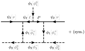
Figure 1: One loop contribution to neutrino masses in the original SVS model. There are in total four diagrams, since (on top of exchanging the internal $\psi_{L}$ and $\ell^{c}$) one can exchange everywhere $\phi_{2}$ with $\phi_{3}$.

In the form just presented, the SVS model is not viable as it cannot accommodate the known neutrino oscillation data. This can be understood as follows. The $\psi_{\ell}\psi_{\ell}\phi_{1}$ interaction is completely anti-symmetric in the flavour indices. This leads to the tree-level prediction of a degenerate light neutrino mass spectrum with eigenvalues $\left(0,m,m\right)$. Since lepton number is violated in the SVS model, one expects that radiative corrections to this tree-level result will generate Majorana neutrino masses and lead to a non-zero splitting of the degenerate states. Figure 1 shows an example. However, in the original SVS model all loop corrections to neutrino masses are necessarily themselves proportional to the $\psi_{\ell}\psi_{\ell}\phi_{1}$ interaction, which is the coupling responsible for the generation of neutrino masses at tree level. (Indeed, any loop contributing to neutrino masses must have an odd number of $\psi_{\ell}\psi_{\ell}\phi_{1}$ interactions.) The 1-loop corrections are then related to the tree-level mass and the relative size of $\delta m_{\nu}^{\rm 1-loop}/m_{\nu}^{\rm tree}$ can be estimated to be at most $\sim\frac{1}{16\pi^{2}}h_{\tau}^{2}\times\cdots<10^{-6}$, where $h_{\tau}$ is the tau Yukawa coupling and the dots stand for other factors which are at most one. We will return to a more explicit calculation of this loop in the next section. For now it suffices to say that neutrino oscillation data requires that the smaller mass splitting in the neutrino sector relative to the larger one must be larger than very roughly $1/6$, in gross contradiction to the above estimate for the original SVS model.

Just for completeness, note that in the diagram of figure 1 the LNV interaction $\phi_{1}\phi_{2}\phi_{3}$ and its conjugate are present, hence the real source of LNV in this case are the $\widetilde{\phi}_{2}^{0}$ and $\widetilde{\phi}_{3}^{0}$ VEVs. This does not, however, mean that the LNV in the trilinear interaction is irrelevant in general. In fact, it is easy to built up diagrams containing $\psi_{\ell}\psi_{\ell}\phi_{1}$, the SM charged current and this trilinear interaction to generate processes such as $e^{-}e^{-}\to 4j$ (or $6j$) at loop-level (tree-level).

2.2 The Pisano-Pleitez-Frampton (PPF) model

Following the generic framework of the SVS model, in 1992 a different 331 model was presented [10, 11]. This model chooses $\beta=-\sqrt{3}$ and thus the third component of the lepton triplet field $\psi_{\ell}$ has charge +1, hence it is identifiable as a right-handed charged lepton — see table 2.

Field	331 representation	$G_{SM}$ decomposition	# flavours	Components	Lepton number
$\psi_{\ell,\alpha}$	$\left(\mathbf{1},\mathbf{3},0\right)$	$\left(\mathbf{1},\widehat{\mathbf{2}},-\frac{1}{2}\right)+\left(\mathbf{1},\widehat{\mathbf{1}},1\right)$	3	$\left(\left(\nu_{\alpha},\ell_{\alpha}\right),\ell_{\alpha}^{c}\right)^{T}$	$\left(1,1,-1\right)^{T}$
$Q_{\alpha=1,2}$	$\left(\mathbf{3},\overline{\mathbf{3}},-\frac{1}{3}\right)$	$\left(\mathbf{3},\widehat{\mathbf{2}},\frac{1}{6}\right)+\left(\mathbf{3},\widehat{\mathbf{1}},-\frac{4}{3}\right)$	2	$\left(\left(d_{\alpha},-u_{\alpha}\right),J_{\alpha}^{c}\right)^{T}$	$\left(0,0,2\right)^{T}$
$Q_{3}$	$\left(\mathbf{3},\mathbf{3},\frac{2}{3}\right)$	$\left(\mathbf{3},\widehat{\mathbf{2}},\frac{1}{6}\right)+\left(\mathbf{3},\widehat{\mathbf{1}},\frac{5}{3}\right)$	1	$\left(\left(t,b\right),J_{3}^{c}\right)^{T}$	$\left(0,0,-2\right)^{T}$
$u_{\alpha}^{c}$	$\left(\overline{\mathbf{3}},\mathbf{1},-\frac{2}{3}\right)$	$\left(\overline{\mathbf{3}},\widehat{\mathbf{1}},-\frac{2}{3}\right)$	3	$u_{\alpha}^{c}$	0
$d_{\alpha}^{c}$	$\left(\overline{\mathbf{3}},\mathbf{1},\frac{1}{3}\right)$	$\left(\overline{\mathbf{3}},\widehat{\mathbf{1}},\frac{1}{3}\right)$	3	$d_{\alpha}^{c}$	0
$J_{\alpha=1,2}$	$\left(\overline{\mathbf{3}},\mathbf{1},\frac{4}{3}\right)$	$\left(\overline{\mathbf{3}},\widehat{\mathbf{1}},\frac{4}{3}\right)$	2	$J_{\alpha}$	-2
$J_{3}$	$\left(\overline{\mathbf{3}},\mathbf{1},-\frac{5}{3}\right)$	$\left(\overline{\mathbf{3}},\widehat{\mathbf{1}},-\frac{5}{3}\right)$	1	$J_{3}$	2
$\phi_{1}$	$\left(\mathbf{1},\mathbf{3},1\right)$	$\left(\mathbf{1},\widehat{\mathbf{2}},\frac{1}{2}\right)+\left(\mathbf{1},\widehat{\mathbf{1}},2\right)$	1	$\left(\left(\phi_{1}^{+},\phi_{1}^{0}\right),\widetilde{\phi}_{1}^{++}\right)^{T}$	$\left(0,0,-2\right)^{T}$
$\phi_{2}$	$\left(\mathbf{1},\mathbf{3},-1\right)$	$\left(\mathbf{1},\widehat{\mathbf{2}},-\frac{3}{2}\right)+\left(\mathbf{1},\widehat{\mathbf{1}},0\right)$	1	$\left(\left(\phi_{2}^{-},\phi_{2}^{--}\right),\widetilde{\phi}_{2}^{0}\right)^{T}$	$\left(2,2,0\right)^{T}$
$\phi_{3}$	$\left(\mathbf{1},\mathbf{3},0\right)$	$\left(\mathbf{1},\widehat{\mathbf{2}},-\frac{1}{2}\right)+\left(\mathbf{1},\widehat{\mathbf{1}},1\right)$	1	$\left(\left(\phi_{3}^{0},\phi_{3}^{-}\right),\widetilde{\phi}_{3}^{+}\right)^{T}$	$\left(0,0,-2\right)^{T}$

Table 2: Field content of the Pisano-Pleitez-Frampton (PPF) model [10, 11].

A central assertion in [10] is that lepton number is violated by charged scalars and gauge bosons. However, we want to stress here that this is not the case. Using the procedure outlined above for the SVS model, the PPF model with the interactions described in [10] preserves the $U(1)_{L}$ symmetry under which the various fields have the charges indicated in table 2, so there is no explicit lepton number violation in the model as written down in [10]. Moreover, unlike the SVS model, here all neutral scalar components have $L=0$ hence there cannot be spontaneous lepton number violation either. Thus the original model of [10] is lepton number conserving. It is important to note, however, that PPF neglected some quartic scalar interactions which are allowed by the gauge symmetry. Most notably it can be shown that the coupling $\phi_{1}\phi_{2}\phi_{3}^{*}\phi_{3}^{*}$, missing in the original paper, violates lepton number by two units.

From now on, we will call the version of this model with the most general gauge invariant Lagrangian the Pisano-Pleitez-Frampton model. This PPF model is indeed lepton number violating. Thus, LNV processes such as neutrinoless double beta decay, will occur. Interestingly, the PPF model, however, does not generate a non-zero neutrino mass. This can be understood by following the possible interactions of the $\psi_{\ell}$ triplet, which contains the SM leptons. Apart from gauge interactions, there is only the $y_{\ell}\psi_{\ell}\psi_{\ell}\phi_{3}$ Yukawa interaction where gauge indices are contracted anti-symmetrically. Hence $y_{\ell}$ must be an anti-symmetric matrix (in flavour space). Yet, one must have an odd number of $y_{\ell}$ matrices along the $\psi_{\ell}$ fermion line in any diagram contributing to a neutrino mass matrix (see figure 2). Hence the flavour matrix $\mathcal{O}$ associated to the effective operator $\mathcal{O}_{\alpha\beta}\psi_{\ell,\alpha}\psi_{\ell,\beta}\times(scalars)$ will always be anti-symmetric (note that the gauge interactions do not change flavour). Thus, no $\nu\nu$ term will be generated at any order of a perturbative expansion.

Figure 2: The only interactions of the $\psi_{\ell}$ multiplet in the PPF model are the ones with the gauge bosons (which do not change flavour) and those of the form $\psi_{\ell}\psi_{\ell}\phi_{3}$, which are anti-symmetric in flavour space. Since an odd number of these latter interactions are needed to build a mass diagram for $\psi_{\ell}$, such a mass must necessarily be flavour anti-symmetric and hence it cannot generate (Majorana) neutrino masses.

That a LNV model can have zero Majorana neutrino masses but a finite half-life for neutrinoless double beta decay, seems to be a contradiction of the well-known “black-box” theorem [76]. However, this apparent contradiction can be traced to another flaw of the PPF model. In it, the $\psi_{\ell}\psi_{\ell}\phi_{3}$ interaction is the only source of charged lepton masses. Its antisymmetry implies that the tree-level charged lepton masses are $(0,m,m)$. (This prediction is analogous to the one for neutrino masses in the SVS model discussed previously.) This is in clear disagreement with the experimentally observed charged lepton masses and thus requires a modification of the PPF model. Moreover, this prediction for the charged lepton spectrum violates the (implicit) assumption in the formulation of the black box theorem [76, 77] that the electron has a non-zero mass. If one follows the procedure given in the original papers on the black box theorem of completing the $0\nu\beta\beta$ decay diagram with charged current interactions, in order to form a Majorana neutrino mass term, one finds that mass insertions are necessary to convert right-handed electrons into left-handed ones. For the PPF model all contributions to $0\nu\beta\beta$ decay produce final states with $e_{L}e_{R}$. The particular prediction for the charged lepton spectrum in this model then leads to an exact zero of the $e_{R}\to e_{L}$ insertions, independent of the flavour compositions of the three mass eigenstates. This is most easily seen for the case where the only non-zero entry in $y_{\ell}$ is $y_{\ell}^{\mu\tau}$. In this case, the massless state is the electron and it is obvious that $e_{R}\to e_{L}$ conversion is impossible. For other cases, the two contributions from the degenerate leptons cancel each other exactly. However, one expects that once that the PPF model has been modified to correct for the unrealistic charged lepton spectrum, non-zero Majorana masses will also automatically appear and the standard form of the black-box theorem is recovered. A discussion of modified PPF models is given below in section 3.

2.3 The Pleitez-Özer (PÖ) model

The generic SVS framework with $\beta=1/\sqrt{3}$ gives rise to the Pleitez-Özer model [71, 72]. In it, the third component of $\psi_{\ell}$ has charge $-1$, so it can be interpreted as the vector partner of the SM right-handed charged leptons $\ell^{c}$ . Since there are 3 flavours of $\psi_{\ell}$, 6 copies of $\ell^{c}$ are then necessary to account for the SM right-handed charged leptons as well as 3 extra vector fermion pairs $\left(\ell^{c},E\right)$. There are no right-handed neutrinos and it can be checked that there is an unbroken global $U(1)_{L}$ (see table 3). Furthermore, none of the neutral scalars carries lepton number, thus there is also no spontaneous violation of lepton number. Neutrinos are therefore massless and the model is not satisfactory from this point of view.

Field	331 representation	$G_{SM}$ decomposition	# flavours	Components	Lepton number
$\psi_{\ell,\alpha}$	$\left(\mathbf{1},\mathbf{3},-\frac{2}{3}\right)$	$\left(\mathbf{1},\widehat{\mathbf{2}},-\frac{1}{2}\right)+\left(\mathbf{1},\widehat{\mathbf{1}},-1\right)$	3	$\left(\left(\nu_{\alpha},\ell_{\alpha}\right),E_{\alpha}\right)^{T}$	$\left(1,1,1\right)^{T}$
$\ell_{\alpha}^{c}$	$\left(\mathbf{1},\mathbf{1},1\right)$	$\left(\mathbf{1},\widehat{\mathbf{1}},1\right)$	6	$\ell_{\alpha}^{c}$	-1
$Q_{\alpha=1,2}$	$\left(\mathbf{3},\overline{\mathbf{3}},\frac{1}{3}\right)$	$\left(\mathbf{3},\widehat{\mathbf{2}},\frac{1}{6}\right)+\left(\mathbf{3},\widehat{\mathbf{1}},\frac{2}{3}\right)$	2	$\left(\left(d_{\alpha},-u_{\alpha}\right),U_{\alpha}\right)^{T}$	$\left(0,0,0\right)^{T}$
$Q_{3}$	$\left(\mathbf{3},\mathbf{3},0\right)$	$\left(\mathbf{3},\widehat{\mathbf{2}},\frac{1}{6}\right)+\left(\mathbf{3},\widehat{\mathbf{1}},-\frac{1}{3}\right)$	1	$\left(\left(t,b\right),D\right)^{T}$	$\left(0,0,0\right)^{T}$
$u_{\alpha}^{c}$	$\left(\overline{\mathbf{3}},\mathbf{1},-\frac{2}{3}\right)$	$\left(\overline{\mathbf{3}},\widehat{\mathbf{1}},-\frac{2}{3}\right)$	5	$u_{\alpha}^{c}$	0
$d_{\alpha}^{c}$	$\left(\overline{\mathbf{3}},\mathbf{1},\frac{1}{3}\right)$	$\left(\overline{\mathbf{3}},\widehat{\mathbf{1}},\frac{1}{3}\right)$	4	$d_{\alpha}^{c}$	0
$\phi_{i=1,2}$	$\left(\mathbf{1},\mathbf{3},\frac{1}{3}\right)$	$\left(\mathbf{1},\widehat{\mathbf{2}},\frac{1}{2}\right)+\left(\mathbf{1},\widehat{\mathbf{1}},0\right)$	2	$\left(\left(\phi_{i}^{+},\phi_{i}^{0}\right),\widetilde{\phi}_{i}^{0}\right)^{T}$	$\left(0,0,0\right)^{T}$
$\phi_{3}$	$\left(\mathbf{1},\mathbf{3},-\frac{2}{3}\right)$	$\left(\mathbf{1},\widehat{\mathbf{2}},-\frac{1}{2}\right)+\left(\mathbf{1},\widehat{\mathbf{1}},-1\right)$	1	$\left(\left(\phi_{3}^{0},\phi_{3}^{-}\right),\widetilde{\phi}_{3}^{-}\right)^{T}$	$\left(0,0,0\right)^{T}$

Table 3: Field content of the Pleitez-Özer model [71, 72], which conserves lepton number.

2.4 Model X

Finally, in the generic SVS framework it is also possible to have $\beta=\sqrt{3}$ — we call this the model X. For this value of $\beta$, the third component of $\psi_{\ell}$ has charge $-2$. Hence we need the $\ell_{X}$ representation (charge +2) shown in table 4 to form a massive, vector fermion pair with this state once the 331 symmetry is broken. The SM right-handed charged leptons are then in a separate representation $\ell^{c}$. It is straightforward to check that this model preserves lepton number, just like the Pleitez-Özer model. So, in the absence of right-handed neutrinos, it predicts massless neutrinos.

Field	331 representation	$G_{SM}$ decomposition	# flavours	Components	Lepton number
$\psi_{\ell,\alpha}$	$\left(\mathbf{1},\mathbf{3},-1\right)$	$\left(\mathbf{1},\widehat{\mathbf{2}},-\frac{1}{2}\right)+\left(\mathbf{1},\widehat{\mathbf{1}},-2\right)$	3	$\left(\left(\nu_{\alpha},\ell_{\alpha}\right),\ell_{X,\alpha}^{c}\right)^{T}$	$\left(1,1,1\right)^{T}$
$\ell_{\alpha}^{c}$	$\left(\mathbf{1},\mathbf{1},1\right)$	$\left(\mathbf{1},\widehat{\mathbf{1}},1\right)$	3	$\ell_{\alpha}^{c}$	-1
$\ell_{X,\alpha}$	$\left(\mathbf{1},\mathbf{1},2\right)$	$\left(\mathbf{1},\widehat{\mathbf{1}},2\right)$	3	$\ell_{X,\alpha}$	-1
$Q_{\alpha=1,2}$	$\left(\mathbf{3},\overline{\mathbf{3}},\frac{2}{3}\right)$	$\left(\mathbf{3},\widehat{\mathbf{2}},\frac{1}{6}\right)+\left(\mathbf{3},\widehat{\mathbf{1}},\frac{5}{3}\right)$	2	$\left(\left(d_{\alpha},-u_{\alpha}\right),J_{\alpha}^{c}\right)^{T}$	$\left(0,0,0\right)^{T}$
$Q_{3}$	$\left(\mathbf{3},\mathbf{3},-\frac{1}{3}\right)$	$\left(\mathbf{3},\widehat{\mathbf{2}},\frac{1}{6}\right)+\left(\mathbf{3},\widehat{\mathbf{1}},-\frac{4}{3}\right)$	1	$\left(\left(t,b\right),J_{3}^{c}\right)^{T}$	$\left(0,0,0\right)^{T}$
$u_{\alpha}^{c}$	$\left(\overline{\mathbf{3}},\mathbf{1},-\frac{2}{3}\right)$	$\left(\overline{\mathbf{3}},\widehat{\mathbf{1}},-\frac{2}{3}\right)$	3	$u_{\alpha}^{c}$	0
$d_{\alpha}^{c}$	$\left(\overline{\mathbf{3}},\mathbf{1},\frac{1}{3}\right)$	$\left(\overline{\mathbf{3}},\widehat{\mathbf{1}},\frac{1}{3}\right)$	3	$d_{\alpha}^{c}$	0
$J_{\alpha=1,2}$	$\left(\overline{\mathbf{3}},\mathbf{1},-\frac{5}{3}\right)$	$\left(\overline{\mathbf{3}},\widehat{\mathbf{1}},-\frac{5}{3}\right)$	2	$J_{\alpha}$	0
$J_{3}$	$\left(\overline{\mathbf{3}},\mathbf{1},\frac{4}{3}\right)$	$\left(\overline{\mathbf{3}},\widehat{\mathbf{1}},\frac{4}{3}\right)$	1	$J_{3}$	0
$\phi_{1}$	$\left(\mathbf{1},\mathbf{3},0\right)$	$\left(\mathbf{1},\widehat{\mathbf{2}},\frac{1}{2}\right)+\left(\mathbf{1},\widehat{\mathbf{1}},-1\right)$	1	$\left(\left(\phi_{1}^{+},\phi_{1}^{0}\right),\widetilde{\phi}_{1}^{-}\right)^{T}$	$\left(0,0,0\right)^{T}$
$\phi_{2}$	$\left(\mathbf{1},\mathbf{3},1\right)$	$\left(\mathbf{1},\widehat{\mathbf{2}},\frac{3}{2}\right)+\left(\mathbf{1},\widehat{\mathbf{1}},0\right)$	1	$\left(\left(\phi_{2}^{++},\phi_{2}^{+}\right),\widetilde{\phi}_{2}^{0}\right)^{T}$	$\left(0,0,0\right)^{T}$
$\phi_{3}$	$\left(\mathbf{1},\mathbf{3},-1\right)$	$\left(\mathbf{1},\widehat{\mathbf{2}},-\frac{1}{2}\right)+\left(\mathbf{1},\widehat{\mathbf{1}},-2\right)$	1	$\left(\left(\phi_{3}^{0},\phi_{3}^{-}\right),\widetilde{\phi}_{3}^{--}\right)^{T}$	$\left(0,0,0\right)^{T}$

Table 4: Field content of the model X, which conserves lepton number.

2.5 The flipped model

All previous four models follow the SVS framework of placing SM lepton doublets in triplets of $SU(3)_{L}$, while quark doublets are spread over one triplet and two anti-triplets. In other words, the extended gauge symmetry discriminates quark families, but not lepton families. Recently [73] we proposed a new model which reverts this scheme: all three quark families are in equal representations, while lepton families are not. To achieve gauge anomaly cancellation and acceptable fermion masses, one of the SM lepton doublets is placed in a sextet of $SU(3)_{L}$, while the rest of the fermions are in singlets, triplets and anti-triplets. As for the scalars, on top of three triplets $\phi_{1,2,3}$, we have introduced a sextet $S$ which plays an important role in the generation of lepton masses, through both tree and loop diagrams. The full field content of the model is reproduced in table 5. Note that this construction requires $\beta=1/\sqrt{3}$.

Field	331 rep.	$G_{SM}$ decomposition	# flav.	Components	Lepton number
$L_{e}$	$\left(\mathbf{1},\mathbf{6},-\frac{1}{3}\right)$	$\begin{array}[]{c}\left(\mathbf{1},\widehat{\mathbf{3}},0\right)+\left(\mathbf{1},\widehat{\mathbf{2}},-\frac{1}{2}\right)\\ +\left(\mathbf{1},\widehat{\mathbf{1}},-1\right)\end{array}$	1	$\left(\begin{array}[]{ccc}\Sigma^{+}&\frac{1}{\sqrt{2}}\Sigma^{0}&\frac{1}{\sqrt{2}}\nu_{e}\\ \frac{1}{\sqrt{2}}\Sigma^{0}&\Sigma^{-}&\frac{1}{\sqrt{2}}\ell_{e}\\ \frac{1}{\sqrt{2}}\nu_{e}&\frac{1}{\sqrt{2}}\ell_{e}&E_{e}\end{array}\right)$	$\left(\begin{array}[]{ccc}-1&-1&1\\ -1&-1&1\\ 1&1&3\end{array}\right)$
$L_{\alpha=\mu,\tau}$	$\left(\mathbf{1},\mathbf{3},-\frac{2}{3}\right)$	$\left(\mathbf{1},\widehat{\mathbf{2}},-\frac{1}{2}\right)+\left(\mathbf{1},\widehat{\mathbf{1}},-1\right)$	2	$\left(\nu_{\alpha},\ell_{\alpha},E_{\alpha}\right)^{T}$	$\left(1,1,3\right)^{T}$
$\ell_{\alpha}^{c}$	$\left(\mathbf{1},\mathbf{1},1\right)$	$\left(\mathbf{1},\widehat{\mathbf{1}},1\right)$	6	$\ell_{\alpha}^{c}$	$-1$
$Q_{\alpha}$	$\left(\mathbf{3},\overline{\mathbf{3}},\frac{1}{3}\right)$	$\left(\mathbf{3},\widehat{\mathbf{2}},\frac{1}{6}\right)+\left(\mathbf{3},\widehat{\mathbf{1}},\frac{2}{3}\right)$	3	$\left(d_{\alpha},-u_{\alpha},U_{\alpha}\right)^{T}$	$\left(0,0,-2\right)^{T}$
$u_{\alpha}^{c}$	$\left(\overline{\mathbf{3}},\mathbf{1},-\frac{2}{3}\right)$	$\left(\overline{\mathbf{3}},\widehat{\mathbf{1}},-\frac{2}{3}\right)$	6	$u_{\alpha}^{c}$	$0$
$d_{\alpha}^{c}$	$\left(\overline{\mathbf{3}},\mathbf{1},\frac{1}{3}\right)$	$\left(\overline{\mathbf{3}},\widehat{\mathbf{1}},\frac{1}{3}\right)$	3	$d_{\alpha}^{c}$	$0$
$\phi_{i=1,2}$	$\left(\mathbf{1},\mathbf{3},\frac{1}{3}\right)$	$\left(\mathbf{1},\widehat{\mathbf{2}},\frac{1}{2}\right)+\left(\mathbf{1},\widehat{\mathbf{1}},0\right)$	2	$\left(H_{i}^{+},H_{i}^{0},\sigma_{i}^{0}\right)^{T}$	$\left(0,0,2\right)^{T}$
$\phi_{3}$	$\left(\mathbf{1},\mathbf{3},-\frac{2}{3}\right)$	$\left(\mathbf{1},\widehat{\mathbf{2}},-\frac{1}{2}\right)+\left(\mathbf{1},\widehat{\mathbf{1}},-1\right)$	1	$\left(H_{3}^{0},H_{3}^{-},\sigma_{3}^{-}\right)^{T}$	$\left(0,0,2\right)^{T}$
$S$	$\left(\mathbf{1},\mathbf{6},\frac{2}{3}\right)$	$\begin{array}[]{c}\left(\mathbf{1},\widehat{\mathbf{3}},1\right)+\left(\mathbf{1},\widehat{\mathbf{2}},\frac{1}{2}\right)\\ +\left(\mathbf{1},\widehat{\mathbf{1}},0\right)\end{array}$	1	$\left(\begin{array}[]{ccc}\Delta^{++}&\frac{1}{\sqrt{2}}\Delta^{+}&\frac{1}{\sqrt{2}}H_{S}^{+}\\ \frac{1}{\sqrt{2}}\Delta^{+}&\Delta^{0}&\frac{1}{\sqrt{2}}H_{S}^{0}\\ \frac{1}{\sqrt{2}}H_{S}^{+}&\frac{1}{\sqrt{2}}H_{S}^{0}&\sigma_{S}^{0}\end{array}\right)$	$\left(\begin{array}[]{ccc}-2&-2&0\\ -2&-2&0\\ 0&0&2\end{array}\right)$

Table 5: Field content of the flipped 331 model [73].

Without making a rigorous fit, we showed in [73] that the model is able to reproduce the observed fermion masses and mixing angles, hence modifications of the model are not mandatory. Here, neutrinos are Majorana particles and therefore lepton number is obviously not conserved by the full Lagrangian. However, if one were to keep only the gauge interactions as well as all the Yukawa interactions allowed by the gauge symmetry, one finds a preserved $U(1)_{L}$ lepton number symmetry, with the associated charges shown in the last column of table 5. As for scalar couplings, most of them also preserve this $U(1)_{L}$, including $\phi_{i}^{*}\phi_{j}\phi_{3}S$ and $\phi_{3}\phi_{3}SS$ which are not self-conjugate. There are only two interactions allowed by the gauge symmetry which break lepton number (by two units): $\phi_{1}\phi_{2}\phi_{3}$ and $\phi_{i}\phi_{j}S^{*}$($i,j=1,2$). In fact, this last one was mentioned in [73] as being important to achieve a realistic neutrino mass matrix. Apart from these two sources of LNV, one also has to consider the VEVs $\left\langle\sigma_{i}^{0}\right\rangle$, $\left\langle\Delta^{0*}\right\rangle$ and $\left\langle\sigma_{S}^{0}\right\rangle$ which all break $U(1)_{L}$ by two units.

2.6 The $E_{6}$ inspired model

The $SU(3)\times SU(3)\times U(1)$ is contained in $SU(3)^{3}$ which in turn is a subgroup of the exceptional $E_{6}$ group. This group has been used in Grand Unified model building [79]. In these models, fermions are in three copies of the fundamental representation $\mathbf{27}$ hence, upon breaking the group down to the $SU(3)\times SU(3)\times U(1)$ subgroup, one ought to obtain a 331 model with family replication in both the lepton and quark sectors. Apart from a possible flip between the $SU(3)$’s representations with their anti-representations, the $E_{6}$ fundamental representation branches as follows:

$$\mathbf{27}\rightarrow\left(\mathbf{1},\mathbf{3},\left[\begin{array}[]{c}2a\\ -a+b\\ -a-b\end{array}\right]\right)+\left(\overline{\mathbf{3}},\mathbf{1},\left[\begin{array}[]{c}-2a\\ a-b\\ a+b\end{array}\right]\right)+\left(\mathbf{3},\overline{\mathbf{3}},0\right)\,,$$ (67)

where the square brackets indicate in an economical way different states with different $U(1)_{X}$ charges, while $a$ and $b$ are parameters describing the linear combination of two $U(1)$’s which form $U(1)_{X}$. So, in order to place the left-handed quarks in $\left(\mathbf{3},\overline{\mathbf{3}},0\right)$, this branching rule implies that one must have $\beta=-1/\sqrt{3}$. In this case, $\left(\mathbf{3},\overline{\mathbf{3}},0\right)$ will also contain the $\left(\mathbf{3},\widehat{\mathbf{1}},-\frac{1}{3}\right)$ SM representation. Hence, from the second term in (67) one must get two $d^{c}$-like states, $\left(\overline{\mathbf{3}},\widehat{\mathbf{1}},\frac{1}{3}\right)$, and one $u^{c}$ like state, $\left(\overline{\mathbf{3}},\widehat{\mathbf{1}},-\frac{2}{3}\right)$. Since the leptons (first term in (67)) have the opposite $X$ charges to these colored states, we shall have two $\left(\mathbf{1},\mathbf{3},-\frac{1}{3}\right)$ representations plus one $\left(\mathbf{1},\mathbf{3},\frac{2}{3}\right)$. Note that any $E_{6}$ model is anomaly free, hence this list of 331 fields is so too. Table 6 contains the overall picture. This model clearly dispels the claim that 331 models predict that the number of generations has to be necessarily equal to the number of colours.

Field	331 representation	$G_{SM}$ decomposition	# flavours	Components	Lepton number
$\psi_{\ell,\alpha}$	$\left(\mathbf{1},\mathbf{3},-\frac{1}{3}\right)$	$\left(\mathbf{1},\widehat{\mathbf{2}},-\frac{1}{2}\right)+\left(\mathbf{1},\widehat{\mathbf{1}},0\right)$	6	$\left(\left(\nu_{\alpha},\ell_{\alpha}\right),N_{\alpha}^{c}\right)^{T}$	$\left(1,1,-1\right)^{T}$
$\psi_{X,\alpha}$	$\left(\mathbf{1},\mathbf{3},\frac{2}{3}\right)$	$\left(\mathbf{1},\widehat{\mathbf{2}},\frac{1}{2}\right)+\left(\mathbf{1},\widehat{\mathbf{1}},1\right)$	3	$\left(\left(E_{X,\alpha},\nu_{X,\alpha}\right),\ell_{\alpha}^{c}\right)^{T}$	$\left(1,1,-1\right)^{T}$
$Q_{\alpha}$	$\left(\mathbf{3},\overline{\mathbf{3}},0\right)$	$\left(\mathbf{3},\widehat{\mathbf{2}},\frac{1}{6}\right)+\left(\mathbf{3},\widehat{\mathbf{1}},-\frac{1}{3}\right)$	3	$\left(\left(d_{\alpha},-u_{\alpha}\right),D_{\alpha}\right)^{T}$	$\left(0,0,2\right)^{T}$
$u_{\alpha}^{c}$	$\left(\overline{\mathbf{3}},\mathbf{1},-\frac{2}{3}\right)$	$\left(\overline{\mathbf{3}},\widehat{\mathbf{1}},-\frac{2}{3}\right)$	3	$u_{\alpha}^{c}$	0
$d_{\alpha}^{c}$	$\left(\overline{\mathbf{3}},\mathbf{1},\frac{1}{3}\right)$	$\left(\overline{\mathbf{3}},\widehat{\mathbf{1}},\frac{1}{3}\right)$	6	$d_{\alpha}^{c}$	0
$\phi_{1}$	$\left(\mathbf{1},\mathbf{3},\frac{2}{3}\right)$	$\left(\mathbf{1},\widehat{\mathbf{2}},\frac{1}{2}\right)+\left(\mathbf{1},\widehat{\mathbf{1}},1\right)$	1	$\left(\left(\phi_{1}^{+},\phi_{1}^{0}\right),\widetilde{\phi}_{1}^{+}\right)^{T}$	$\left(0,0,-2\right)^{T}$
$\phi_{i=2,3}$	$\left(\mathbf{1},\mathbf{3},-\frac{1}{3}\right)$	$\left(\mathbf{1},\widehat{\mathbf{2}},-\frac{1}{2}\right)+\left(\mathbf{1},\widehat{\mathbf{1}},0\right)$	2	$\left(\left(\phi_{i}^{0},\phi_{i}^{-}\right),\widetilde{\phi}_{i}^{0}\right)^{T}$	$\left(0,0,-2\right)^{T}$

Table 6: Field content of the $E_{6}$ inspired 331 model [74].

This 331 model was first studied by Sánchez, Ponce and Martinéz in [74]. They considered a scalar sector with three triplet fields with the same quantum numbers as the scalars in the SVS model. With this field content, there are no sources of explicit lepton number violation, but the electroweak singlet components $\widetilde{\phi}_{2,3}^{0}$ inside the two $\phi_{2,3}$ triplets do lead to spontaneous LNV (see table 6).

While we will not do a complete flavour fit of this model to all experimental data, we shall briefly describe how it is possible to obtain realistic lepton masses. To start, consider the notation $\left\langle\phi_{1}\right\rangle=\left(0,k_{1},0\right)^{T}$, $\left\langle\phi_{2,3}\right\rangle=\left(k_{2,3},0,n_{2,3}\right)^{T}$ and note that the only allowed interactions between $\psi_{\ell}$, $\psi_{X}$ and the scalars are

$$\mathscr{L} =\cdots+y_{\ell\ell}\psi_{\ell}\psi_{\ell}\phi_{1}+y_{\ell X}^{(2)}\psi_{\ell}\psi_{X}\phi_{2}+y_{\ell X}^{(3)}\psi_{\ell}\psi_{X}\phi_{3}+\textrm{h.c.}+\cdots\,.$$ (68)

Here, $y_{\ell\ell}$ stands for a square $6\times 6$ matrix, while $y_{\ell X}^{(i)}$ are two rectangular $6\times 3$ matrices. Hence, considering only the colorless leptons,

$$\left\langle\mathscr{L}\right\rangle_{\textrm{lepton mass}}=m_{\ell,\alpha\beta}\Psi_{\alpha}^{\ell}\Psi_{\beta}^{\ell^{c}}+m_{\nu,\alpha\beta}\Psi_{\alpha}^{\nu}\Psi_{\beta}^{\nu}$$

with

$$M_{\nu}=2\left(\begin{array}[]{ccc}0&k_{1}y_{\ell\ell}&-n_{2}y_{\ell X}^{(2)}-n_{3}y_{\ell X}^{(3)}\\ \cdot&0&k_{2}y_{\ell X}^{(2)}+k_{3}y_{\ell X}^{(3)}\\ \cdot&\cdot&0\end{array}\right)\,,$$ (72)

$$M_{\ell}=\left(\begin{array}[]{cc}n_{2}y_{\ell X}^{(2)}+n_{3}y_{\ell X}^{(3)}&,-k_{2}y_{\ell X}^{(2)}-k_{3}y_{\ell X}^{(3)}\end{array}\right)\,,$$ (74)

in the basis $\Psi^{\nu}=\left(\nu_{\alpha},N_{\alpha}^{c},\nu_{X,\beta}\right)^{T}$, $\Psi^{\ell}=\left(\ell_{\alpha}\right)$ and $\Psi^{\ell^{c}}=\left(E_{X,\beta},\ell_{\beta}^{c}\right)^{T}$ ($\alpha=1,\cdots,6$; $\beta=1,\cdots,3$).

A careful analysis of the neutrino mass matrix reveals that, baring the existence of special alignments and/or cancellations, one expects the following mass eigenstates:

• Three light Majorana neutrino states $\nu_{M}$ with seesaw masses $\mathcal{O}\left(y_{\ell\ell}k_{1}k_{i}/n_{i}\right)$, $i=2,3$, and composed almost entirely of $N^{c}$ states;

• Three quasi-Dirac neutrino pairs $\nu_{lQD}$ with masses $\mathcal{O}\left(y_{\ell\ell}k_{1}\right)$ composed of a ~50%/50% admixture of $N^{c}$ and $\nu$ states;

• Three quasi-Dirac heavy neutrino pairs $\nu_{hQD}$ with masses $\mathcal{O}\left(y_{\ell X}^{(i)}n_{i}\right)$ composed of a ~50%/50% admixture of $\nu$ and $\nu_{X}$ states.

This rough estimation holds true only if there is a clear hierarchy between these sets of neutrino masses: $y_{\ell X}^{(i)}n_{i}\gg y_{\ell\ell}k_{1}\gg y_{\ell\ell}k_{1}k_{i}/n_{i}$ ($i=2,3$). However, in this limit the three seesawed neutrinos are mostly singlets under the SM gauge group, hence they cannot play the role of the observed active neutrinos. That role must then be played by the three quasi-Dirac neutrino pairs $\nu_{lQD}$ with masses proportional to the value of the coupling matrix $y_{\ell\ell}$ and the VEV $k_{1}$. Even though we will not write down the precise expressions for the neutrino masses and lepton mixing angles, it is possible to have sub-eV active neutrinos $\nu_{lQD}$, at the price of choosing small $\mathcal{O}\left(10^{-12}\right)$ entries in the matrix $y_{\ell\ell}$. This choice does not affect the mass of the remaining active neutrinos $\nu_{hQD}$, which must have masses above the SM $Z^{0}$ mass, in order not to be in conflict with the measured invisible width of the $Z^{0}$ boson. One must then additionally ensure that the light Majorana neutrino states $\nu_{M}$ do not mix significantly with the $\nu_{lQD}$ states.

As for charged leptons, the $M_{\ell}$ matrix will have rank 3 if the matrix $n_{2}y_{\ell X}^{(2)}+n_{3}y_{\ell X}^{(3)}$ is proportional to $k_{2}y_{\ell X}^{(2)}+k_{3}y_{\ell X}^{(3)}$, and this is an interesting limit as it would imply that 3 of the charged leptons are massless ($e$, $\mu$, $\tau$), so a small departure from this scenario can actually be used to explain the ratio $m_{\tau}/m_{W,Z}$. Finally, since the quark Yukawa coupling matrices are free parameters, the quark masses and mixing parameters can easily be fitted in this model. Since the $E_{6}$-inspired model can, in principle, explain the observed fermion masses, we will not discuss extended versions of this 331 model.

3 Simple extensions of the SVS, PPF, PÖ and X models

Four of the basic 331 models discussed above fail to produce a viable neutrino mass spectrum. These four follow the basic framework of the SVS model and we called them SVS, PPF, PÖ and X in the previous section. The PPF model moreover predicts a charged lepton spectrum in disagreement with experimental data, see table 7 for a summary. The table also recalls, as discussed above, that lepton number is actually conserved in models PÖ and X.

Issue	SVS	PPF	PÖ	X
$U(1)_{L}$ violation?	✓	✓	✗	✗
$\nu$ masses?	✓	✗	✗	✗
Correct $\nu$ masses?	✗	✗	✗	✗
Correct $\ell$ masses?	✓	✗	✓	✓

Table 7: A summary of lepton number violation and problems with the lepton sector in four of the basic 331 models discussed in section 2.

To fix these problems, in the following we consider 4 simple extensions of the field content for these basic models:

• Add a fermionic particle, $N^{\prime c}$, singlet under the 331 symmetry group.

• Add a scalar sextet $S$ such that $\psi_{\ell}\psi_{\ell}S$ provides a symmetric contribution to the neutrino and charged leptons mass matrix.

• Add a vector-like pair $\left(E^{c},E\right)$ of charged leptons.

• Add a $\phi_{X}$ triplet scalar field in order to generate the interaction $\psi_{\ell}\psi_{\ell}\phi_{X}$.

However, not all of these extensions work equally well for all models, see table 8. Here, extensions which will fix the problems with the lepton spectra for a particular model are marked with (✓), while those that do not work are marked with (✗). The cases which fail can be understood as follows:

• Adding right-handed neutrinos to the PPF model leads to the generation of neutrino masses, but it does not fix the charged lepton mass problem.

• Both the PPF and SVS models already contain a $\psi_{\ell}\psi_{\ell}\phi_{i}$ interaction, so adding another $\phi_{X}$ scalar does not lead to a qualitative change of these models.

• Models PÖ and X already contain vector-like leptons, hence adding another pair is again unhelpful. Furthermore, adding the vector fermions $\left(E^{c},E\right)$ to the SVS model is also unsatisfactory.

Having said this, we now turn to a detailed discussion of the effects of the model extensions which do work.

Modification	PPF	SVS	PÖ	X
$+N^{\prime c}$	✗	✓	✓	✓
$+S$	✓	✓	✓	✓
$+E^{c},E$	✓	✗	✗	✗
$+\phi_{X}$	✗	✗	✓	✓

Table 8: Simple extensions of the four models (PPF, SVS, PÖ, X) which will fix (✓) the problems with the lepton spectra summarized in table 7. Cases that will not work are marked with (✗). For explanation see text.

3.1 Extended PPF models

We start our discussion with the PPF model. Adding a fermion singlet $N^{\prime c}$ to the PPF model allows an interaction term $\psi_{\ell}N^{\prime c}\phi_{3}^{*}$ (and a mass term $N^{\prime c}N^{\prime c}$). Since this addition does not affect the charged lepton spectrum, by itself such extension of the PPF model is insufficient and we will thus not discuss it here (but see below for other models).

Adding a scalar sextet, on the other hand, provides a valid fix for the PPF model. Consider $S=\left(\mathbf{1},\mathbf{6},0\right)$:

$$S=\begin{pmatrix}\Delta^{0}&\frac{1}{\sqrt{2}}\Delta^{-}&\frac{1}{\sqrt{2}}H^{+}\\ \frac{1}{\sqrt{2}}\Delta^{-}&\Delta^{--}&\frac{1}{\sqrt{2}}H^{0}\\ \frac{1}{\sqrt{2}}H^{+}&\frac{1}{\sqrt{2}}H^{0}&\sigma^{++}\end{pmatrix}\,.$$ (75)

The components denoted as $\Delta$, $H$, and $\sigma$ form a triplet, a doublet, and a singlet respectively under the $SU(2)_{L}$ group. The interaction of the lepton triplet with this sextet contains the terms

$$y_{S}\psi_{\ell,\alpha}S^{*}\psi_{\ell,\beta}=y_{S}\left[\nu_{\alpha}\nu_{\beta}\Delta^{0*}+\frac{1}{\sqrt{2}}(\ell_{\alpha}\ell^{c}_{\beta}+\ell^{c}_{\alpha}\ell_{\beta})H^{0*}+\cdots\right]\,.$$ (76)

The term proportional to $\Delta^{0*}$ will give a type-II seesaw contribution to the neutrino masses, once $\Delta^{0}$ acquires a VEV, proportional to $m_{\alpha\beta}^{\nu}=(y_{S})_{\alpha\beta}\langle\Delta^{0}\rangle$, while the charged lepton mass matrix is now the sum of two terms: $m^{\ell}=y_{\ell}\langle\phi^{0}_{3}\rangle+y_{S}\langle H^{0}\rangle$. It is easy to see that in the absence of $y_{S}$ the mass spectrum for the charged leptons has the eigenvalues ($0,m,m$). Thus, in order to achieve the correct hierarchies for $e$, $\mu$ and $\tau$, the second term in $m^{\ell}$ must dominate. This puts a lower limit on the largest entries in $y_{S}\langle H^{0}\rangle$ of the order of the $\tau$ mass.

Since the same $y_{S}$ appears in neutrino masses, one must have $\langle\Delta^{0}\rangle/\langle H^{0}\rangle\raise 1.29167pt\hbox{$\;<$\kern-7.5pt\raise-4.73611pt\hbox{$\sim\;$}}10^{-10}$ for a correct explanation of neutrino data. Adding a sextet to the original PPF model was already proposed in [66]. These authors, however, argued that such a small ratio calls for a protecting symmetry. The proposed symmetry eliminates all lepton number violating scalar interactions from the model: in addition to the original term $\phi_{1}\phi_{2}\phi_{3}^{*}\phi_{3}^{*}$, these are $\phi_{3}\phi_{3}S^{*}$ and $SSS$. Since under this condition lepton number is conserved, neutrinos are massless again. Thus, with the addition of only a sextet to the original PPF model, we have to accept the fine-tuning between the triplet and doublet VEVs if we are to explain neutrino data. We note in passing that such a small ratio of VEVs might be due to a small parameter in the scalar potential, such as the coefficient of $\phi_{3}\phi_{3}S^{*}$.

Figure 3: One-loop diagrams in the PPF model, extended with a vector-like lepton.

We now turn to the third possibility in our list. Both problems, neutrino and charged lepton masses, can be cured in the PPF model by the introduction of a pair of vector-like charged leptons, $E$ and $E^{c}$, in the representations $\left(\mathbf{1},\mathbf{1},\mp 1\right)$. In the original PPF model, the Lagrangian contains the interaction terms

$${\mathscr{L}=\cdots+\frac{1}{2}y_{\ell,\alpha\beta}\psi_{\ell,\alpha}\psi_{\ell,\beta}\phi_{3}+\lambda_{7}\phi_{1}\phi_{2}\phi_{3}^{*}\phi_{3}^{*}+\textrm{h.c.}\,,}$$ (77)

and introducing the left-handed Weyl spinors $E$ and $E^{c}$ makes it possible to write down the following also

$$\mathscr{L}_{EE^{c}}=h_{E^{c},\alpha}\psi_{\ell,\alpha}E^{c}\phi_{1}^{*}+h_{E,\alpha}\psi_{\ell,\alpha}{E}\phi_{2}^{*}+m_{EE^{c}}E{E^{c}}\,.$$ (78)

The charged lepton mass matrix, after symmetry breaking, becomes:

$$M_{\ell E}=\begin{pmatrix}0&y_{\ell,e\mu}k_{3}&y_{\ell,e\tau}k_{3}&h_{E^{c},e}k_{1}\\ -y_{\ell,e\mu}k_{3}&0&y_{\ell,\mu\tau}k_{3}&h_{E^{c},\mu}k_{1}\\ -y_{\ell,e\tau}k_{3}&-y_{\ell,\mu\tau}k_{3}&0&h_{E^{c},\tau}k_{1}\\ h_{E,e}n_{2}&h_{E,\mu}n_{2}&h_{E,\tau}n_{2}&m_{EE^{c}}\end{pmatrix}.$$ (79)

Here, $k_{1}$, $k_{3}$ and $n_{2}$ are the VEVs of $\phi^{0}_{1}$, $\phi^{0}_{3}$ and ${\widetilde{\phi}}^{0}_{2}$, respectively. We now define $|y_{\ell}|=\sqrt{y_{\ell,e\mu}^{2}+y_{\ell,e\tau}^{2}+y_{\ell,\mu\tau}^{2}}$, $|h_{E^{c}}|=\sqrt{\sum_{\alpha}(h_{E^{c},\alpha})^{2}}$ and $|h_{{E}}|=\sqrt{\sum_{\alpha}(h_{{E,\alpha}})^{2}}$. Then, in the limit $|h_{E^{c}}|=|h_{{E}}|\to 0$ we obtain the original result for the charged lepton masses, given by: $m_{1,2,3}=(-|y_{\ell}|k_{3},0,|y_{\ell}|k_{3})$. Note that the massless state has the eigenvector $e_{2}=\frac{1}{|y_{\ell}|}(y_{\ell,\mu\tau},y_{\ell,e\tau},1)^{T}$. In other words, a good starting point to have the electron as the lightest state corresponds to the choice $y_{\ell,e\mu},y_{\ell,e\tau}\ll y_{\ell,\mu\tau}$. Note that $|y_{\ell}|\to 0$ is not allowed, since in this case the matrix $M_{\ell E}$ in equation (79) only has 2 non-zero eigenvalues. In this limit, the lighter of the two non-zero mass states is given by $m=|h_{{E}}||h_{{E^{c}}}|k_{1}n_{2}/m_{EE^{c}}$. For values of $m_{EE^{c}}={\cal O}$(TeV) and $n_{2}={\cal O}$(TeV), fitting $m_{\tau}$ then requires $|h_{E}|\times|h_{E^{c}}|\sim{\cal O}(10^{-2})$. For non-zero values of $|h_{E}|$, $|h_{E^{c}}|$ and $y_{\ell}$ the mass degeneracy is broken and a realistic charged lepton spectrum can be easily obtained for $|y_{\ell}|\raise 1.29167pt\hbox{$\;<$\kern-7.5pt\raise-4.73611pt\hbox{$\sim\;$}}{\cal O}(10^{-2}-10^{-3})$ together with $|y_{\ell}|<|h_{E}||h_{E^{c}}|$ (and $k_{1}\sim k_{3}$).

Extending the PPF model with a vector-like lepton does not only solve the charged lepton mass problem, but it also leads to the generation of 1-loop neutrino masses — see figure 3. For these loops, in addition to the terms given in equation (78), the two interactions terms in equation (77) are needed. As explained in the previous section, in the minimal PPF model lepton number violation is proportional to $\lambda_{7}$ and, thus, all loops that generate a Majorana neutrino mass must contain this particular quartic vertex. Such statement is still true once $E$ and $E^{c}$ are added to the model, hence this important scalar interaction is present in all diagrams show in figure 3.

We will give a rough estimate of the size of these loops. A complete calculation would require rotating all internal states in the diagrams to the mass eigenstate basis and then summing over all states. However, since (i) the mass of the vector-like lepton has to be much larger than the mass of the tau and (ii) $\lambda_{7}$ has to be small, as shown below, we can estimate the relative contributions of each diagram in figure 3 to the neutrino mass individually. Let’s concentrate on diagram (c) first. It’s contribution to the neutrino mass matrix is estimated to be:

$$(m_{\nu})_{\alpha\beta}=\frac{1}{16\pi^{2}}\sin 2\theta_{S}m_{EE^{c}}\Delta B_{0}\left[h_{E,\alpha}h_{E^{c},\beta}+(\alpha\leftrightarrow\beta)\right]\,.$$ (80)

Here, $\theta_{S}$ is the angle that diagonalizes the (2,2) submatrix of the charged scalars,

$$M^{2}_{\phi_{1}\phi_{2}}=\begin{pmatrix}m_{\phi_{1}}^{2}&\lambda_{7}k_{3}^{2}\\ \lambda_{7}k_{3}^{2}&m_{\phi_{2}}^{2}\end{pmatrix}\,,$$ (81)

and is given by

$$\sin 2\theta_{S}=\frac{2\lambda_{7}k_{3}^{2}}{m_{1}^{2}-m_{2}^{2}}\,,$$ (82)

with $m_{1,2}^{2}$ being the eigenvalues of $M^{2}_{\phi_{1}\phi_{2}}$. In equation (80) $\Delta B_{0}$ stands for the difference between the two 1-loop $B_{0}$ functions for the two scalar mass eigenstates and it reads

$$\Delta B_{0}=\frac{m_{1}^{2}\log(m_{1}^{2}/m_{EE^{c}}^{2})}{m_{1}^{2}-m_{EE^{c}}^{2}}-\frac{m_{2}^{2}\log(m_{2}^{2}/m_{EE^{c}}^{2})}{m_{2}^{2}-m_{EE^{c}}^{2}}\,.$$ (83)

Since we know experimentally that neutrino masses are small, while the mass of the vector-like lepton should be larger than several 100’s of GeV, either the Yukawa couplings or the factor $\sin 2\theta_{S}\Delta B_{0}$ should be small. The former is not an option in the present model, since only for $|h_{E}||h_{{E^{c}}}|\sim{\cal O}(10^{-2})$ a realistic charged lepton spectrum can be obtained, as discussed above.

We define:

$${\overline{M}}= \;\frac{1}{2}\left(m_{1}+m_{2}\right)\,,$$ (84)

$$\Delta M= \;\left(m_{2}-m_{1}\right)\,.$$ (85)

Then, in the limit of $\Delta M\ll{\overline{M}}$ and for $m_{EE^{c}}<{\overline{M}}$, $\sin 2\theta_{S}\Delta B_{0}$ becomes simply $\sim(\lambda_{7}k_{3}^{2})/{\overline{M}}^{2}$, so the neutrino mass is roughly given by the expression

$$m_{\nu}\sim\left(\frac{m_{EE^{c}}}{\rm TeV}\right)\left(\frac{\rm TeV}{{\overline{M}}^{2}}\right)^{2}\left(\frac{k_{3}}{100\hskip 2.84526pt{\rm GeV}}\right)^{2}\left(\frac{|h_{E^{c}}||h_{{\bar{E}^{c}}}|}{10^{-2}}\right)\left(\frac{\lambda_{7}}{10^{-7}}\right)10^{-1}\hskip 2.84526pt{\rm eV}\,.$$ (86)

We now turn to a brief discussion of the relative importance of the diagrams (a)–(c) in figure 3. Diagrams (a) and (b) contain the same parameters as diagram (c) just discussed and, furthermore, they also depend on the other doublet VEV in the model ($k_{1}$) as well as the couplings $y_{\ell,\alpha\beta}$. Assuming that the Yukawas $h_{E,\alpha}$ and $h_{E^{c},\beta}$ are very roughly of the same order of magnitude numerically, the relative importance of the three diagrams can then be estimated to be

$$(c):(a):(b)=1:|y_{\ell}|\frac{k_{1}}{k_{3}}:\left(|y_{\ell}|\frac{k_{1}}{k_{3}}\right)^{2}\,.$$ (87)

The ratio $\frac{k_{1}}{k_{3}}$ is not fixed in this model, therefore $k_{3}$ can be smaller than $k_{1}$. Only the combination $\sqrt{k_{1}^{2}+k_{3}^{2}}=v=174$ GeV is fixed. However, as discussed above, the tau mass constrains the combination $|h_{E}||h_{E^{c}}|k_{3}$ to be of the GeV order, for $n_{2}\simeq m_{EE^{c}}$ of the TeV order. For Yukawa couplings in the perturbative regime, this means that $k_{3}$ can not be much smaller than 1 GeV. Thus, diagram (c) is usually the dominant one, and the other diagrams can be at most equally important, if $k_{3}$ is pushed to its lower limit.

Before moving on, we recall that adding additional triplet scalars, without adding ($E,E^{c}$), does not provide a valid solution for the PPF model, see table 8.

3.2 Extended SVS models

For the SVS model, two of the four possibilities listed in table 8 will be valid solutions: (i) adding a fermion singlet $N^{\prime c}$ and (ii) adding a scalar sextet.

Adding (three copies) of $N^{\prime c}$, in addition to the term $y_{\ell}\psi_{\ell}\psi_{\ell}\phi_{1}$, one can write down three new Lagrangian terms for the (extended) SVS model:

$$\mathscr{L}=\sum_{j=2,3}y^{(j)}_{N^{\prime}}\psi_{\ell}N^{\prime c}\phi_{j}^{*}+\mu N^{\prime c}N^{\prime c}\,.$$ (88)

In the basis ($\nu,N^{c},N^{\prime c}$), the neutrino mass matrix becomes

$$M^{\nu}=\begin{pmatrix}0&m_{D}&m_{L}\\ m_{D}^{T}&0&M_{R}\\ m_{L}^{T}&M_{R}^{T}&\mu\end{pmatrix}.$$ (89)

Here, $m_{D}=y_{\ell}k_{1}$, $m_{L}=\sum_{j}y^{(j)}_{N^{\prime}}k_{j}$, $M_{R}=\sum_{j}y^{(j)}_{N^{\prime}}n_{j}$ and $\mu$ are $3\times 3$ matrices. There are two limits for $\mu$. For $M_{R}\ll\mu$ the matrix in equation (89) will lead to a double seesaw, in other words, integrating out $N^{\prime c}$ would give a Majorana mass entry in the (2,2) position of the above matrix of the order of $M_{R}\mu^{-1}M_{R}^{T}$. If $\mu\ll M_{R}$, the matrix gives neutrinos a mass via the inverse seesaw mechanism

$$m_{\nu}=m_{D}(M_{R}^{T})^{-1}\mu M_{R}^{-1}m_{D}^{T}\,.$$ (90)

The fit to neutrino masses can easily be done. This case has been studied in [80]. Note that if $\mu=0$ there is no linear seesaw contribution proportional to $m_{L}$. Indeed, in a model such as this one where $m_{L}\propto M_{R}$ and $m_{D}^{T}=-m_{D}$, one has:

$$m_{D}(M_{R}^{T})^{-1}m_{L}+\left[m_{D}(M_{R}^{T})^{-1}m_{L}\right]^{T}=0\,.$$ (91)

Such limit $\mu=0$ can be achieved with some additional symmetry, as discussed in [14]. However, neutrinos will still acquire mass at 1-loop level via, for example, the diagram shown in figure 1, and also via the gauge loops discussed in [14]. Consider first the loop shown in figure 1. The loop will vanish in the limit where the coefficient $\rho$ of the term $\phi_{1}\phi_{2}\phi_{3}$ vanishes. The calculation is very similar to the loop discussed for the PPF model, with some modifications: $m_{EE^{c}}$ has to be replaced by the SM charged lepton masses and the Yukawa matrices appearing at the vertices are $y_{\ell}$ and $y_{\ell\ell^{c}}$, where the latter is the matrix entering the charged lepton mass matrix. If $\rho/{\overline{M}}$ is a small number, where ${\overline{M}}$ is some average mass of the scalars, we very roughly estimate that

$$m_{\nu} \;\sim\frac{2}{16\pi^{2}}m_{\tau}\frac{k}{n}\left(\frac{\rho}{{\overline{M}}}\right)^{2}\left(\frac{n}{{\overline{M}}}\right)^{2}|y_{\ell}||y_{\ell\ell^{c}}|$$ (92)

$$\;\sim 0.05\Big{(}\frac{\rho/{\overline{M}}}{10^{-2}}\Big{)}^{2}\frac{|y_{\ell}|}{10^{-2}}\frac{|y_{\ell\ell^{c}}|}{10^{-2}}\hskip 2.84526pt{\rm eV}\,$$ (93)

for $k_{i}\simeq k\sim 100$ GeV and $n_{i}\simeq n\sim 1$ TeV.

The gauge loops discussed in [14] are more subtle. In the SVS model, in addition to the trilinear coupling $\rho$, the VEVs $n_{2}$ and $n_{3}$ also violate lepton number. Thus, once the 331 symmetry is broken, there exists a mixing between gauge bosons that leads to lepton number violating processes. In particular, one can draw the diagrams shown in figure 4. Note that the VEV insertions indicated at the top of these diagrams always are in the combination $k_{2}n_{2}$ and/or $k_{3}n_{3}$, i.e. they correspond to a $\Delta(L)=2$ effect.

The diagram on the left shows the contribution to the neutrino mass in the basis where the internal fermions are mass eigenstates. One can understand this propagator as an infinite series of mass insertions, as indicated by the diagrams to the right. The first term in this expansion is proportional to $m_{D}$, which is completely antisymmetric, and thus does not give any contribution. However, higher order terms will come proportional to powers of $f=(m_{D}M_{R}^{*}M_{R}-M_{R}M_{R}^{\dagger}m_{D})$, which in general is non-zero. It is interesting to note that, for the special case where the heavy Dirac-pairs start out degenerate ($M_{R}\propto\mathbb{1}$), the commutator $f$ vanishes and the gauge loops go to zero. In the general case, where $f$ is not much smaller than $M_{R}M_{R}^{\dagger}m_{D}$ this gauge loop will dominate over the scalar loop and put a constraint on $m_{D}M_{R}^{-1}$ to be typically below $10^{-8}$ or so.

Figure 4: Gauge loops in the extended SVS model. The full neutrino propagator with the mass eigenstates $\Psi^{(\nu)}_{n}$ can be expanded in a series of mass insertions. The first non-zero term involves three mass insertions (see text).

Adding a sextet $S$ with the quantum numbers $\left(\mathbf{1},\mathbf{6},2/3\right)$ also may solve the neutrino mass problem. The components of such a field can be written as in equation (75), with the only difference being the electric charges. The part of the Lagrangian involving $S$ contains the following important terms:

$$\mathscr{L}=\cdots+y_{S}(\Delta^{0}\nu\nu+\sqrt{2}H^{0}\nu N^{c}+\sigma^{0}N^{c}N^{c})+\textrm{h.c.}\,.$$ (94)

If all the VEVs of $\Delta^{0}$, $H^{0}$ and $\sigma^{0}$ are non-zero, the light neutrino masses have both seesaw type-I and type-II contributions. One just needs to ensure that $\langle\Delta^{0}\rangle\sim\textrm{eV}\ll\langle H^{0}\rangle\sim\textrm{100 GeV}\ll\langle\sigma^{0}\rangle\sim\textrm{TeV}$.

3.3 Extending the PÖ and X models

The situation is rather simpler in models PÖ and X, which both conserve lepton number. They also do not have neutrino singlets, hence they predict that neutrinos are massless. Here, we will very briefly discuss the different extended versions of these models, commenting also on the differences with respect to the models SVS and PPF. Since models PÖ and X are very similar in this respect, we discuss both at the same time.

Adding three copies of fermion singlets $N^{c}$ makes it possible to write down the terms

$$\mathscr{L}=y_{\nu}\psi_{\ell}N^{c}\phi_{3}^{*}+M_{N}N^{c}N^{c}\,.$$ (95)

Note that, since the triplet $\psi_{\ell}$ does not contain a $N^{c}$ in neither model PÖ nor model X, this will give an ordinary seesaw mechanism of type-I (to be compared with the inverse or double seesaw in the SVS model) which is sufficient to explain neutrino data.

Adding a sextet $S$, with the quantum numbers $\left(\mathbf{1},\mathbf{6},-4/3\right)$ in the case of model PÖ and $\left(\mathbf{1},\mathbf{6},2\right)$ in case of model X, gives rise to Majorana neutrino masses once the neutral component $\Delta^{0}$ of the $SU(2)_{L}$ scalar triplet contained in $S$ acquires a VEV. This is a pure seesaw type-II contribution since $\Delta^{0}$ is the only neutral component of these sextets.

Finally, neutrino masses can be generated at the 1-loop level also in the models PÖ and X, by introducing an additional triplet scalar $\phi_{X}$. The required quantum numbers are $\left(1,\mathbf{3},4/3\right)$ (model PÖ) and $\left(1,\mathbf{3},2\right)$ (model X). The resulting Feynman diagram, in the Pleitez-Özer model, is shown in figure 5. In both models the calculation of the loop and the resulting constraints on model parameters are very similar to the results discussed above for models PPF and SVS, with some obvious replacements.

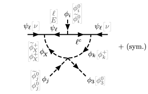
Figure 5: Scalar loop for neutrino masses in the Pleitez-Özer model extended with a scalar triplet $\phi_{X}$. In fact, two distinct diagrams are possible, depending on which components inside the square brackets are picked (either the ones on top, or the ones at the bottom). Analogous loops can be made for model X with an added $\phi_{X}$ scalar triplet.

4 Conclusions

We have studied in a systematic way the status of lepton number in 331 models. The fact that lepton number often does not commute with the extended $SU(3)_{C}\times SU(3)_{L}\times U(1)_{X}$ gauge group makes this an interesting topic, leading to the existence of gauge bosons and colored fermions with a non-zero $U(1)_{L}$ charge and, potentially, to lepton number violation. Note also that the 331 symmetry may break to the Standard Model gauge group at a relatively low energy scale ($\sim$TeV), in which case the LHC would be able to probe the sources of lepton number violation.

However, as we have made clear in this work, there is a large diversity of 331 models, and in some of them lepton number not only commutes with the gauge group, but it is also preserved by the full Lagrangian and VEVs of the scalars. These are nevertheless exceptional cases; in general it is possible to (a) write down sets of gauge invariant interactions which do not preserve any global $U(1)_{L}$ and/or (b) have neutral scalar components with a non-zero lepton number which break spontaneously this symmetry.

Most of the models we discuss, in their original form, are unable to explain the observed lepton masses and neutrino oscillation data. For these models we have listed several simple extensions which can accommodate all lepton data (some of them had already been proposed previously by other authors). As such, any of these extended models can be used for further study.

We have focused mainly on the generation of acceptable neutrino masses (and mixing angles), having mentioned lepton number violating processes, such as neutrinoless double beta decay, only in passing when it was most relevant. Elsewhere [81], we shall provide a more detailed analysis of this process, both in 331 models as well as in other models with an extended gauge groups.

Appendix: decomposition of 331 representations

The decomposition of the most relevant $SU(3)_{L}\times U(1)_{X}$ representations into $SU(2)_{L}\times U(1)_{Y}$ representations has already been provided in equations (2)–(4). As such, in this appendix we simply clarify how the components of these representations are related.

A triplet $\mathbf{3}$ of $SU(3)_{L}$ breaks into a doublet $\widehat{\mathbf{2}}$ plus a singlet $\widehat{\mathbf{1}}$ of $SU(2)_{L}$. Noting that the electric charge of each component depends on the $U(1)_{X}$ charge of the triplet, as well as the $\beta$ parameter as shown in equation (2), we may simply label the components of $\widehat{\mathbf{2}}$ by their isopin ($1/2$ and $-1/2$). We can then settle with the following identification:

$$\mathbf{3} =\left(\begin{array}[]{c}\widehat{\mathbf{2}}_{1/2}\\ \widehat{\mathbf{2}}_{-1/2}\\ \widehat{\mathbf{1}}\end{array}\right)\,.$$ (99)

From here we infer that an anti-triplet $\overline{\mathbf{3}}$ of $SU(3)_{L}$, which also decomposes into a doublet $\widehat{\mathbf{2}}$ plus a singlet $\widehat{\mathbf{1}}$ must be written as

$$\overline{\mathbf{3}} =\left(\begin{array}[]{c}\widehat{\mathbf{2}}_{-1/2}\\ -\widehat{\mathbf{2}}_{1/2}\\ \widehat{\mathbf{1}}\end{array}\right)\,.$$ (103)

A (anti)sextuplet $\mathbf{6}$ of $SU(3)_{L}$ breaks into a triplet $\widehat{\mathbf{3}}$, a doublet $\widehat{\mathbf{2}}$ and a singlet $\widehat{\mathbf{1}}$ of $SU(2)_{L}$. These representations ($\mathbf{6}$ and $\overline{\mathbf{6}}$) are often pictured as matrices instead of vectors, since that makes their contraction with triplets more intuitive. For example, if $\overline{\mathbf{6}}_{ij}\mathbf{3}{}_{i}\mathbf{3}^{\prime}_{j}$ is gauge invariant, one must have the following identification:

$$\mathbf{6}=\left(\begin{array}[]{ccc}\widehat{\mathbf{3}}_{1}&\frac{1}{\sqrt{2}}\widehat{\mathbf{3}}_{0}&\frac{1}{\sqrt{2}}\widehat{\mathbf{2}}_{1/2}\\ \frac{1}{\sqrt{2}}\widehat{\mathbf{3}}_{0}&\widehat{\mathbf{3}}_{-1}&\frac{1}{\sqrt{2}}\widehat{\mathbf{2}}_{-1/2}\\ \frac{1}{\sqrt{2}}\widehat{\mathbf{2}}_{1/2}&\frac{1}{\sqrt{2}}\widehat{\mathbf{2}}_{-1/2}&\widehat{\mathbf{1}}\end{array}\right)\,,\; \overline{\mathbf{6}}=\left(\begin{array}[]{ccc}\widehat{\mathbf{3}}_{-1}&-\frac{1}{\sqrt{2}}\widehat{\mathbf{3}}_{0}&\frac{1}{\sqrt{2}}\widehat{\mathbf{2}}_{-1/2}\\ -\frac{1}{\sqrt{2}}\widehat{\mathbf{3}}_{0}&\widehat{\mathbf{3}}_{1}&-\frac{1}{\sqrt{2}}\widehat{\mathbf{2}}_{1/2}\\ \frac{1}{\sqrt{2}}\widehat{\mathbf{2}}_{-1/2}&-\frac{1}{\sqrt{2}}\widehat{\mathbf{2}}_{1/2}&\widehat{\mathbf{1}}\end{array}\right)\,.$$ (110)

A mass terms $\textrm{Tr}\left(\overline{\mathbf{6}}^{\prime}\cdot\mathbf{6}\right)$ then translates into $\textrm{Tr}\left(\overline{\Delta}^{\prime}\cdot\Delta\right)+\widehat{\mathbf{2}}^{\prime}_{-1/2}\widehat{\mathbf{2}}{}_{1/2}-\widehat{\mathbf{2}}^{\prime}_{1/2}\widehat{\mathbf{2}}{}_{-1/2}+\widehat{\mathbf{1}}^{\prime}\widehat{\mathbf{1}}$ for two $SU(2)_{L}$ triplets $\Delta$ and $\overline{\Delta}^{\prime}$ which we can write in terms of isospin components as

$$\overline{\Delta}^{\prime}=\left(\begin{array}[]{cc}\widehat{\mathbf{3}}^{\prime}_{-1}&-\frac{1}{\sqrt{2}}\widehat{\mathbf{3}}^{\prime}_{0}\\ -\frac{1}{\sqrt{2}}\widehat{\mathbf{3}}^{\prime}_{0}&\widehat{\mathbf{3}}^{\prime}_{1}\end{array}\right)\,,\; \Delta=\left(\begin{array}[]{cc}\widehat{\mathbf{3}}_{1}&\frac{1}{\sqrt{2}}\widehat{\mathbf{3}}_{0}\\ \frac{1}{\sqrt{2}}\widehat{\mathbf{3}}_{0}&\widehat{\mathbf{3}}_{-1}\end{array}\right)\,.$$ (115)

Note that conventions in the literature vary regarding the signs in front of some of the triplet components $\widehat{\mathbf{3}}_{i}$, since these might change with a rephasing of fields components. However, the $\frac{1}{\sqrt{2}}$ factors cannot be absorbed, so the expression in equation (110) for the sextet differs in a material way from the one used in [66, 13, 17], for example, agreeing instead with [16].

Finally, we consider what happens to gauge bosons $W_{L,i}$ ($i=1,\cdots 8$) which are in the adjoint representation ($\mathbf{8}$) of $SU(3)_{L}$. The representation $\left(\mathbf{8},0\right)$ of $SU(3)_{L}\times U(1)_{X}$ breaks into one $SU(2)_{L}$ triplet $\widehat{\mathbf{3}}$, one singlet $\widehat{\mathbf{1}}$ and two doublets $\widehat{\mathbf{2}}$ and $\widehat{\mathbf{2}}^{\prime}$ with opposite hypercharges; for definiteness let us consider $\widehat{\mathbf{2}}$ to be the one with $y=\frac{\sqrt{3}}{2}\beta$ — see equation (4). Contractions with (anti)triplets are done in the standard way ($\mathbf{8}_{ij}\overline{\mathbf{3}}{}_{i}\mathbf{3}_{j}$), resulting in the following identification of the octet components:

$$\mathbf{8} =\left(\begin{array}[]{ccc}\frac{1}{\sqrt{6}}\widehat{\mathbf{1}}-\frac{1}{\sqrt{2}}\widehat{\mathbf{3}}_{0}&\widehat{\mathbf{3}}_{1}&-\widehat{\mathbf{2}}_{1/2}\\ -\widehat{\mathbf{3}}_{-1}&\frac{1}{\sqrt{6}}\widehat{\mathbf{1}}+\frac{1}{\sqrt{2}}\widehat{\mathbf{3}}_{0}&-\widehat{\mathbf{2}}_{-1/2}\\ -\widehat{\mathbf{2}}^{\prime}_{-1/2}&\widehat{\mathbf{2}}^{\prime}_{1/2}&-\sqrt{\frac{2}{3}}\widehat{\mathbf{1}}\end{array}\right)$$ (119)

In the case of gauge bosons, we are dealing with a real field transforming as $\mathbf{8}$ hence the $SU(2)_{L}$ $\widehat{\mathbf{2}}$ and $\widehat{\mathbf{2}}^{\prime}$ doublets are not independent. Indeed, one can alternatively write $\mathbf{8}=\frac{1}{\sqrt{2}}W^{a}\lambda^{a}$, where $\lambda^{1,\cdots,8}$ are the Gell-Mann matrices:

$$\mathbf{W}_{L} =\frac{1}{\sqrt{2}}\left(\begin{array}[]{ccc}W_{L}^{3}+\frac{1}{\sqrt{3}}W_{L}^{8}&W_{L}^{1}-iW_{L}^{2}&W_{L}^{4}-iW_{L}^{5}\\ W_{L}^{1}+iW_{L}^{2}&-W_{L}^{3}+\frac{1}{\sqrt{3}}W_{L}^{8}&W_{L}^{6}-iW_{L}^{7}\\ W_{L}^{4}+iW_{L}^{5}&W_{L}^{6}+iW_{L}^{7}&-\frac{2}{\sqrt{3}}W_{L}^{8}\end{array}\right)\,.$$ (123)

Equating the expressions in equations (119) and (123), we get the identification

$$\left(\begin{array}[]{c}\widehat{\mathbf{3}}_{1}\\ \widehat{\mathbf{3}}_{0}\\ \widehat{\mathbf{3}}_{-1}\end{array}\right)=\left(\begin{array}[]{c}\widehat{\mathbf{3}}_{-1}^{*}\\ \widehat{\mathbf{3}}_{0}^{*}\\ \widehat{\mathbf{3}}_{1}^{*}\end{array}\right) =\left(\begin{array}[]{c}\left(W_{L}^{1}-iW_{L}^{2}\right)/\sqrt{2}\\ -W_{L}^{3}\\ \left(W_{L}^{1}+iW_{L}^{2}\right)/\sqrt{2}\end{array}\right)\,,$$ (133)

$$\left(\begin{array}[]{c}\widehat{\mathbf{2}}_{1/2}\\ \widehat{\mathbf{2}}_{-1/2}\end{array}\right)=\left(\begin{array}[]{c}\widehat{\mathbf{2}}_{-1/2}^{\prime*}\\ -\widehat{\mathbf{2}}_{1/2}^{\prime*}\end{array}\right) =\left(\begin{array}[]{c}\left(-W_{L}^{4}+iW_{L}^{5}\right)/\sqrt{2}\\ \left(-W_{L}^{6}+iW_{L}^{7}\right)/\sqrt{2}\end{array}\right)\,,$$ (140)

$$\widehat{\mathbf{1}} =W_{L}^{8}\,.$$ (141)

It is then obvious that the Standard Model $SU(2)_{L}$ gauge bosons correspond to the triplet $\widehat{\mathbf{3}}$ (i.e., $W_{L}^{1,2,3}$) while the singlet $\widehat{\mathbf{1}}$ (i.e., $W_{L}^{8}$) mixes with the $U\left(1\right)_{X}$ gauge boson $W_{X}$ to form the $U(1)_{Y}$ gauge boson $B$:

$$B =\frac{1}{\sqrt{g_{L}^{2}+g_{X}^{2}\beta^{2}}}\left(g_{X}\beta W_{L}^{8}+g_{L}W_{X}\right)\,.$$ (142)

In this expression, $g_{L}$ and $g_{X}$ stand for the gauge coupling constants of $SU(3)_{L}$ and $U\left(1\right)_{X}$, which are related to $g_{Y}$ through the relation

$$g_{Y}^{-2} =\beta^{2}g_{L}^{-2}+g_{X}^{-2}\,.$$ (143)

Finally, note that the charge of the various components of $\mathbf{W}_{L}$ depend only on $\beta$:

$$Q\left(\mathbf{W}_{L}\right)_{\beta} =\left(\begin{array}[]{ccc}0&+&0\\ -&0&-\\ 0&+&0\end{array}\right)_{\!\!\!-\frac{1}{\sqrt{3}}},\,\left(\begin{array}[]{ccc}0&+&+\\ -&0&0\\ -&0&0\end{array}\right)_{\!\!\!\frac{1}{\sqrt{3}}},\,\left(\begin{array}[]{ccc}0&+&-\\ -&0&--\\ +&++&0\end{array}\right)_{\!\!\!-\sqrt{3}},\,\left(\begin{array}[]{ccc}0&+&++\\ -&0&+\\ --&-&0\end{array}\right)_{\!\!\!\sqrt{3}}\,.$$ (156)

References

- [1] H. Georgi and S. Glashow, Unity of all elementary-particle forces, Phys. Rev. Lett. 32 (1974) 438–441.
- [2] H. Georgi, The state of the art — gauge theories, AIP Conf. Proc. 23 (1975) 575–582.
- [3] H. Fritzsch and P. Minkowski, Unified interactions of leptons and hadrons, Annals Phys. 93 (1975) 193–266.
- [4] F. Gürsey, P. Ramond and P. Sikivie, A universal gauge theory model based on , Phys. Lett. B60 (1976) 177–180.
- [5] J. C. Pati and A. Salam, Lepton number as the fourth "color", Phys.Rev. D10 (1974) 275–289; Erratum Phys. Rev. D 11, 703 (1975).
- [6] R. Mohapatra and J. C. Pati, "Natural" left-right symmetry, Phys.Rev. D11 (1975) 2558.
- [7] R. N. Mohapatra and G. Senjanovic, Neutrino masses and mixings in gauge models with spontaneous parity violation, Phys. Rev. D23 (1981) 165.
- [8] R. M. Fonseca, On the chirality of the SM and the fermion content of GUTs, Nucl. Phys. B897 (2015) 757–780, arXiv:1504.03695 [hep-ph].
- [9] M. Singer, J. Valle and J. Schechter, Canonical neutral-current predictions from the weak-electromagnetic gauge group , Phys. Rev. D 22 (1980) 738.
- [10] F. Pisano and V. Pleitez, model for electroweak interactions, Phys. Rev. D 46 (1992) 410–417, arXiv:hep-ph/9206242.
- [11] P. H. Frampton, Chiral dilepton model and the flavor question, Phys. Rev. Lett. 69 (1992) 2889–2891.
- [12] T. Kitabayashi and M. Yasue, Radiatively induced neutrino masses and oscillations in an gauge model, Phys. Rev. D63 (2001) 095002, arXiv:hep-ph/0010087 [hep-ph].
- [13] M. B. Tully and G. C. Joshi, Generating neutrino mass in the 3-3-1 model, Phys. Rev. D64 (2001) 011301, arXiv:hep-ph/0011172 [hep-ph].
- [14] S. M. Boucenna, S. Morisi and J. W. F. Valle, Radiative neutrino mass in 3-3-1 scheme, Phys. Rev. D90 (2014) 1 013005, arXiv:1405.2332 [hep-ph].
- [15] S. M. Boucenna, R. M. Fonseca, F. Gonzalez-Canales and J. W. F. Valle, Small neutrino masses and gauge coupling unification, Phys. Rev. D91 (2015) 3 031702, arXiv:1411.0566 [hep-ph].
- [16] C. A. d. S. Pires, Neutrino mass mechanisms in 3-3-1 models: a short review, Physics International 6 1 (2015) 33–41, arXiv:1412.1002 [hep-ph].
- [17] H. Okada, N. Okada and Y. Orikasa, Radiative seesaw mechanism in a minimal 3-3-1 model, Phys. Rev. D93 (2016) 7 073006, arXiv:1504.01204 [hep-ph].
- [18] Y. Okamoto and M. Yasue, Radiatively generated neutrino masses in gauge models, Phys. Lett. B466 (1999) 267–273, arXiv:hep-ph/9906383 [hep-ph].
- [19] J. C. Montero, C. A. de S. Pires and V. Pleitez, Lepton masses from a TeV scale in a 3-3-1 model, Phys. Rev. D66 (2002) 113003, arXiv:hep-ph/0112203 [hep-ph].
- [20] J. C. Montero, C. A. De S. Pires and V. Pleitez, Neutrino masses through the seesaw mechanism in 3-3-1 models, Phys. Rev. D65 (2002) 095001, arXiv:hep-ph/0112246 [hep-ph].
- [21] J. C. Montero, V. Pleitez and M. C. Rodriguez, Supersymmetric 3-3-1 model with right-handed neutrinos, Phys. Rev. D70 (2004) 075004, arXiv:hep-ph/0406299 [hep-ph].
- [22] H. Okada, N. Okada and Y. Orikasa, Radiative seesaw mechanism in a minimal 3-3-1 model, Phys. Rev. D93 (2016) 7 073006, arXiv:1504.01204 [hep-ph].
- [23] P. V. Dong, H. N. Long and D. V. Soa, Neutrino masses in the economical 3-3-1 model, Phys. Rev. D75 (2007) 073006, arXiv:hep-ph/0610381 [hep-ph].
- [24] T. Kitabayashi and M. Yasuè, Two-loop radiative neutrino mechanism in an gauge model, Phys. Rev. D63 (2001) 095006.
- [25] H. N. Long, model with right-handed neutrinos, Phys. Rev. D53 (1996) 437–445, arXiv:hep-ph/9504274 [hep-ph].
- [26] R. Foot, H. N. Long and T. A. Tran, and gauge models with right-handed neutrinos, Phys. Rev. D50 (1994) 34–38, arXiv:hep-ph/9402243 [hep-ph].
- [27] D. Chang and H. N. Long, Interesting radiative patterns of neutrino mass in an model with right-handed neutrinos, Phys. Rev. D73 (2006) 053006, arXiv:hep-ph/0603098 [hep-ph].
- [28] D. A. Gutiérrez, W. A. Ponce and L. A. Sánchez, Phenomenology of the model with right-handed neutrinos, Eur. Phys. J. C46 (2006) 497–509, arXiv:hep-ph/0411077 [hep-ph].
- [29] G. Tavares-Velasco and J. J. Toscano, Static quantities of a neutral bilepton in the 331 model with right-handed neutrinos, Phys. Rev. D70 (2004) 053006, arXiv:hep-ph/0407047 [hep-ph].
- [30] H. N. Long and V. T. Van, Quark family discrimination and flavor changing neutral currents in the model with right-handed neutrinos, J. Phys. G25 (1999) 2319–2324, arXiv:hep-ph/9909302 [hep-ph].
- [31] J. K. Mizukoshi, C. A. de S. Pires, F. S. Queiroz and P. S. Rodrigues da Silva, WIMPs in a 3-3-1 model with heavy sterile neutrinos, Phys. Rev. D83 (2011) 065024, arXiv:1010.4097 [hep-ph].
- [32] A. E. Cárcamo Hernández and R. Martinez, A predictive 3-3-1 model with flavor symmetry, Nucl. Phys. B905 (2016) 337–358, arXiv:1501.05937 [hep-ph].
- [33] A. E. C. Hernàndez and R. Martinez, Fermion mass and mixing pattern in a minimal T7 flavor 331 model, J. Phys. G43 (2016) 4 045003, arXiv:1501.07261 [hep-ph].
- [34] V. V. Vien and H. N. Long, The flavor symmetry in 3-3-1 model with neutral leptons, JHEP 04 (2014) 133, arXiv:1402.1256 [hep-ph].
- [35] A. E. C. Hernández, E. C. Mur and R. Martinez, Lepton masses and mixing in models with a flavor symmetry, Phys. Rev. D90 (2014) 7 073001, arXiv:1407.5217 [hep-ph].
- [36] A. E. C. Hernández, R. Martinez and J. Nisperuza, discrete group as a source of the quark mass and mixing pattern in 331 models, Eur. Phys. J. C75 (2015) 2 72, arXiv:1401.0937 [hep-ph].
- [37] V. V. Vien and H. N. Long, The flavor symmery in 3-3-1 model with neutral leptons, Int. J. Mod. Phys. A28 (2013) 1350159, arXiv:1312.5034 [hep-ph].
- [38] F. Yin, Neutrino mixing matrix in the 3-3-1 model with heavy leptons and symmetry, Phys. Rev. D75 (2007) 073010, arXiv:0704.3827 [hep-ph].
- [39] P. V. Dong, H. N. Long, C. H. Nam and V. V. Vien, flavor symmetry in 3-3-1 models, Phys. Rev. D85 (2012) 053001, arXiv:1111.6360 [hep-ph].
- [40] P. V. Dong, H. N. Long, D. V. Soa and V. V. Vien, The 3-3-1 model with flavor symmetry, Eur. Phys. J. C71 (2011) 1544, arXiv:1009.2328 [hep-ph].
- [41] P. V. Dong, L. T. Hue, H. N. Long and D. V. Soa, The 3-3-1 model with flavor symmetry, Phys. Rev. D81 (2010) 053004, arXiv:1001.4625 [hep-ph].
- [42] A. G. Dias, C. A. de S. Pires and P. S. R. da Silva, Discrete symmetries, invisible axion and lepton number symmetry in an economic 3-3-1 model, Phys. Rev. D68 (2003) 115009, arXiv:hep-ph/0309058 [hep-ph].
- [43] A. E. Cárcamo Hernández, R. Martínez and F. Ochoa, Fermion masses and mixings in the 3-3-1 model with right-handed neutrinos based on the flavor symmetry (2013), arXiv:1309.6567 [hep-ph].
- [44] A. J. Buras, S. Uhlig and F. Schwab, Waiting for precise measurements of and , Rev. Mod. Phys. 80 (2008) 965–1007, arXiv:hep-ph/0405132 [hep-ph].
- [45] A. J. Buras, F. De Fazio and J. Girrbach, 331 models facing new data, JHEP 02 (2014) 112, arXiv:1311.6729 [hep-ph].
- [46] G. A. González-Sprinberg, R. Martínez and O. Sampayo, Bilepton and exotic quark mass limits in 331 models from decay, Phys. Rev. D71 (2005) 115003, arXiv:hep-ph/0504078 [hep-ph].
- [47] J. Agrawal, P. H. Frampton and J. T. Liu, The decay in the 3-3-1 model, Int. J. Mod. Phys. A11 (1996) 2263–2280, arXiv:hep-ph/9502353 [hep-ph].
- [48] A. J. Buras, F. De Fazio, J. Girrbach and M. V. Carlucci, The anatomy of quark flavour observables in 331 models in the flavour precision era, JHEP 02 (2013) 023, arXiv:1211.1237 [hep-ph].
- [49] C. Promberger, S. Schatt and F. Schwab, Flavor-changing neutral current effects and CP violation in the minimal 3-3-1 model, Phys. Rev. D75 (2007) 115007, arXiv:hep-ph/0702169 [hep-ph].
- [50] J. A. Rodriguez and M. Sher, Flavor-changing neutral currents and rare B decays in 3-3-1 models, Phys. Rev. D70 (2004) 117702, arXiv:hep-ph/0407248 [hep-ph].
- [51] A. J. Buras, F. De Fazio and J. Girrbach-Noe, Z-Z’ mixing and Z-mediated FCNCs in models, JHEP 08 (2014) 039, arXiv:1405.3850 [hep-ph].
- [52] S. M. Boucenna, S. Morisi and A. Vicente, LHC diphoton resonance from gauge symmetry, Phys. Rev. D93 (2016) 115008, arXiv:1512.06878 [hep-ph].
- [53] P. V. Dong and N. T. K. Ngan, Phenomenology of the simple 3-3-1 model with inert scalars (2015), arXiv:1512.09073 [hep-ph].
- [54] Q.-H. Cao et al., The diphoton excess, low energy theorem, and the 331 model, Phys. Rev. D93 (2016) 7 075030, arXiv:1512.08441 [hep-ph].
- [55] S. F. Mantilla, R. Martinez, F. Ochoa and C. F. Sierra, Diphoton decay for a 750 GeV scalar boson in a model (2016), arXiv:1602.05216 [hep-ph].
- [56] A. E. C. Hernandez and I. Nisandzic, LHC diphoton 750 GeV resonance as an indication of gauge symmetry (2015), arXiv:1512.07165 [hep-ph].
- [57] R. Martinez, F. Ochoa and C. F. Sierra, models in view of the 750 GeV diphoton signal (2016), arXiv:1606.03415 [hep-ph].
- [58] Y. A. Coutinho, V. Salustino Guimarães and A. A. Nepomuceno, Bounds on Z’ from 3-3-1 model at the LHC energies, Phys. Rev. D87 (2013) 11 115014, arXiv:1304.7907 [hep-ph].
- [59] J. E. C. Montalvo et al., Search for the Higgs boson at LHC in 3-3-1 model, Phys. Rev. D88 (2013) 9 095020, arXiv:1311.0845 [hep-ph].
- [60] F. Richard, A interpretation of data and consequences for high energy colliders (2013), arXiv:1312.2467 [hep-ph].
- [61] G. M. Pelaggi, A. Strumia and E. Vigiani, Trinification can explain the di-photon and di-boson LHC anomalies, JHEP 03 (2016) 025, arXiv:1512.07225 [hep-ph].
- [62] P. V. Dong and N. T. K. Ngan, Phenomenology of the simple 3-3-1 model with inert scalars (2015), arXiv:1512.09073 [hep-ph].
- [63] A. Nepomuceno, B. Meirose and F. Eccard, First results on bilepton production based on LHC collision data and predictions for run II (2016), arXiv:1604.07471 [hep-ph].
- [64] C. Coriano and P. H. Frampton, X-events and their interpretation (2016), arXiv:1606.08713 [hep-ph].
- [65] H. Okada, N. Okada, Y. Orikasa and K. Yagyu, Higgs phenomenology in the minimal model, Phys. Rev. D94 (2016) 1 015002, arXiv:1604.01948 [hep-ph].
- [66] R. Foot, O. F. Hernandez, F. Pisano and V. Pleitez, Lepton masses in an gauge model, Phys. Rev. D47 (1993) 4158–4161, arXiv:hep-ph/9207264 [hep-ph].
- [67] J. T. Liu and D. Ng, Lepton-flavor-changing processes and CP violation in the model, Phys. Rev. D50 (1994) 548–557, arXiv:hep-ph/9401228 [hep-ph].
- [68] D. Ng, The Electroweak theory of , Phys. Rev. D49 (1994) 4805–4811, arXiv:hep-ph/9212284 [hep-ph].
- [69] T. V. Duong and E. Ma, Supersymmetric gauge model: Higgs structure at the electroweak energy scale, Phys. Lett. B316 (1993) 307–311, arXiv:hep-ph/9306264 [hep-ph].
- [70] J. C. Montero, C. A. de S. Pires, V. Pleitez, Seesaw tau lepton mass and calculable neutrino masses in a 3-3-1 model, Phys. Rev. D65 (2002) 093017, arXiv:hep-ph/0103096.
- [71] V. Pleitez, New fermions and a vector-like third generation in models, Phys. Rev. D53 (1996) 514–526, arXiv:hep-ph/9412304 [hep-ph].
- [72] M. Özer, model of the electroweak interactions without exotic quarks, Phys. Rev. D54 (1996) 1143–1149.
- [73] R. M. Fonseca and M. Hirsch, A flipped 331 model (2016), JHEP 08 (2016) 003, arXiv:1606.01109 [hep-ph].
- [74] L. A. Sánchez, W. A. Ponce and R. Martinez, as an subgroup, Phys. Rev. D64 (2001) 075013, arXiv:hep-ph/0103244 [hep-ph].
- [75] J. W. F. Valle and M. Singer, Lepton number violation with quasi Dirac neutrinos, Phys. Rev. D28 (1983) 540.
- [76] J. Schechter and J. W. F. Valle, Neutrinoless double- decay in theories, Phys. Rev. D25 (1982) 2951.
- [77] E. Takasugi, Can the neutrinoless double beta decay take place in the case of Dirac neutrinos?, Phys. Lett. B149 (1984) 372–376.
- [78] J. C. Montero, F. Pisano and V. Pleitez, Neutral currents and Glashow-Iliopoulos-Maiani mechanism in models for electroweak interactions, Phys. Rev. D47 (1993) 2918–2929, arXiv:hep-ph/9212271 [hep-ph].
- [79] F. Gursey, P. Ramond and P. Sikivie, A universal gauge theory model based on , Phys. Lett. B60 (1976) 177–180.
- [80] S. M. Boucenna, J. W. F. Valle and A. Vicente, Predicting charged lepton flavor violation from 3-3-1 gauge symmetry, Phys. Rev. D92 (2015) 5 053001, arXiv:1502.07546 [hep-ph].
- [81] R. M. Fonseca and M. Hirsch, Gauge vectors and double beta decay, IFIC/16-50 (in preparation).