Universal features of quantum bounce in loop quantum cosmology

Abstract

In this Letter, we study analytically the evolutions of the flat Friedmann-Lemaitre-Robertson-Walker (FLRW) universe and its linear perturbations in the framework of the dressed metric approach in loop quantum cosmology (LQC). Assuming that the evolution of the background is dominated by the kinetic energy of the inflaton at the quantum bounce, we find that both evolutions of the background and its perturbations are independent of the inflationary potentials during the pre-inflationary phase. During this period the effective potentials of the perturbations can be well approximated by a Pöschl-Teller (PT) potential, from which we find analytically the mode functions and then calculate the corresponding Bogoliubov coefficients at the onset of the slow-roll inflation, valid for any inflationary model with a single scalar field. Imposing the Bunch-Davies (BD) vacuum in the contracting phase prior to the bounce when the modes are all inside the Hubble horizon, we show that particles are generically created due to the pre-inflation dynamics. Matching them to those obtained in the slow-roll inflationary phase, we investigate the effects of the pre-inflation dynamics on the scalar and tensor power spectra and find features that can be tested by current and forthcoming observations. In particular, to be consistent with the Planck 2015 data, we find that the universe must have expanded at least $141$ e-folds since the bounce.

I Introduction

The paradigm of cosmic inflation has achieved remarkable successes in solving several problems of the standard big bang cosmology and predicting the primordial perturbation spectra whose evolutions explain both the formation of the large scale structure of the universe and the small inhomogeneities in the cosmic microwave background (CMB) inflation . Now they are matched to observations with unprecedented precisions WMAP ; Planck2013 ; Planck2015 . However, such successes are contingent on the understanding of physics in much earlier epochs when energies were about the Planck scale. This leads to several conceptual issues. For example, to be consistent with observations, the universe must have expanded at least $60$ e-folds during its inflationary phase. However, if the universe had expanded a little bit more than $70$ e-folds during inflation (as it is the case in a large class of inflationary models MRV ), then one can show that the wavelengths of all fluctuation modes which are currently inside the Hubble radius were smaller than the Planck length at the beginning of the period of inflation. This was referred to as the trans-Planckian issue in trans-planck , and leads to the question about the validity of the assumption: the matter fields are quantum in nature but the spacetime is still classical, which are used at the beginning of inflation in order to make predictions inflation . In addition, insisting on the use of general relativity (GR) to describe the inflationary process will inevitably lead to an initial singularity singularity . Moreover, the inflation paradigm usually sets the BD vacuum state at the time when the wavelength of fluctuations were well within the Hubble horizon during the inflationary process. However, such treatment ignores the pre-inflationary dynamics which could lead to non-BD states at the onset of inflation, even when these modes were well inside the Hubble horizon during inflation. For more detail about the sensibility of the inflationary paradigm to Planckian physics, we refer the readers to trans-planck ; DB .

All the issues mentioned above are closely related to the fact that we are working in the regime where GR is known to break down. One believes that new physics in this regime - a quantum theory of gravity, will provide a complete description of inflation as well as its pre-inflationary dynamics. LQC is one of such theories that offers a framework to address these issues, in which the inflationary scenarios can be extended from the onset of the slow-roll inflation back to the Planck scale in a self-consistent way planck_extension ; planck_extension_CQG ; quadratic_loop . Remarkably, the quantum geometry effects of LQC at the Planck scale provide a natural resolution of the big bang singularity (see bounce ; Ashtekar2015CQG ; BB16 ; Yang_alternative_2009 and references therein). In such a picture, the singularity is replaced by a quantum bounce, and the universe that starts at the bounce can eventually evolve to the desired slow-roll inflation AS10 ; bounce_inflation ; bounce_inflation2 ; deformed_tensor ; deformed_scalar ; deformed ; Starobinsky_loop ; bounce_effects . An important question now is whether the quantum bounce can leave any observational signatures to current/forth-coming observations, so LQC can be placed directly under experimental tests. The answer to this question is affirmative. In fact, with some (reasonable) assumptions and choice of the initial conditions, the deformed algebra approach already leads to inconsistence with current observations deformed . Note that in general there are two main approaches to implement cosmological perturbations in the framework of LQC, the dressed metric and deformed algebra approaches bounce ; Ashtekar2015CQG ; BB16 . In both, the primordial perturbations have been intensively studied numerically planck_extension_CQG ; quadratic_loop ; bounce_effects ; deformed ; deformed_scalar ; deformed_tensor ; Starobinsky_loop .

One of our purposes of this Letter, in contrast to the previous numerical studies, is to present an analytical analysis of the effects of the quantum bounce and pre-inflation dynamics on the evolutions of both background and spectra of the scalar and tensor perturbations, in the framework of the dressed metric approach (planck_extension, ; planck_extension_CQG, ; quadratic_loop, ). It is expected that such an analysis will provide a more complete understanding of the problem and deeper insights. In the following, we will focus on the case that the kinetic energy of the inflaton dominates the evolutions at the bounce, because a potential dominated bounce is either not able to produce the desired slow-roll inflation Starobinsky_loop , or leads to a large amount of e-folds of expansion. This will wash out all the observational information about the pre-inflation dynamics and the resulting perturbations are the same as those given in GR (bounce, ; Ashtekar2015CQG, ; BB16, ). Assuming that the influence of the potential at the bounce is negligible, our studies show that:

• During the pre-inflationary phase, the evolutions of the background and the scalar and tensor perturbations are independent of the inflationary potentials. Thus, the evolution of the background is the same for any chosen potential, and in this sense we say that it is universal.

• During this phase the potentials of the scalar and tensor perturbations can be well approximated by an effective PT potential, for which analytic solutions of the mode functions can be found. The Bogoliubov coefficients at the onset of the slow-roll inflation can thereby be calculated [cf. (III)], which are valid for any slow-roll inflationary model with a single scalar field. Assuming that the universe is in the BD vacuum in the contracting phase (the moments where $t\lesssim-t_{s}$ as shown in Fig. 2) we find that particle creations occur generically during the pre-inflation phase.

• Oscillations always happen in the power spectra, and their phases for both scalar and tensor perturbations are the same, in contrast to other theories of quantum gravity trans-planck ; Zhu1 .

• Fitting the power spectra to the Planck 2015 data Planck2015 , we find the lower bound for $N_{\text{tot}}\equiv\ln{(a_{0}/a_{B})}>141$ (95% C.L.), where $a_{B}$ and $a_{0}$ denote the expansion factor at the bounce and current time, respectively. Details of the calculations will be reported elsewhere bounce_uniform .

II Quantum Bounce

In LQC, the semi-classical dynamics of a flat FLRW universe with a single scalar field $\phi$ and potential $V(\phi)$ is described by planck_extension ; planck_extension_CQG ; quadratic_loop ,

$$H^{2}=\frac{8\pi}{3m_{\text{Pl}}^{2}}\rho\left(1-\frac{\rho}{\rho_{\text{c}}}\right),$$ (1)

$$\ddot{\phi}+3H\dot{\phi}+V_{,\phi}=0,$$ (2)

where $H\equiv\dot{a}/a$ is the Hubble parameter, a dot denotes the derivative with respect to the cosmic time $t$, and $\rho_{c}$ is the maximum energy density, with $\rho\equiv\dot{\phi}^{2}/2+V(\phi)\leq\rho_{c}$. Eq. (1) shows that the big bang singularity now is replaced by a non-singular quantum bounce at $\rho=\rho_{\text{c}}$ [cf. Fig. 1]. The background evolution has been extensively studied, and one of the main results is that, following the bounce, a desired slow-roll inflation phase is almost inevitable, provided that the evolution is dominated initially by the kinetic energy of the scalar field at the quantum bounce bounce ; bounce_inflation ; bounce_inflation2 ; Starobinsky_loop . In this Letter, we will focus on this case. Then, ignoring the potential term $V(\phi)$, from Eqs. (1) and (2) we find

$$a(t)=a_{\text{B}}\left(1+\gamma_{B}\frac{t^{2}}{t_{\text{Pl}}^{2}}\right)^{1/6},$$ (3)

where $a_{\text{B}}\equiv a(t_{B}),\gamma_{B}\equiv{24\pi\rho_{\text{c}}}/{m_{\text{Pl}}^{4}}$, and $t_{\text{Pl}}$ denotes the Planck time. In writing the above expression we also set $t_{\text{B}}=0$. In Fig. 1 we display the above analytical solution and the equation of state

$$w_{\phi}\equiv\frac{\dot{\phi}^{2}-2V(\phi)}{\dot{\phi}^{2}+2V(\phi)},$$ (4)

together with several numerical solutions of $a(t)$ for different potentials. From this figure, specially the curves of $w_{\phi}$, we can see that the universe experiences three different phases: bouncing, transition, and slow-roll inflation. During the bouncing phase, $w_{\phi}$ remains almost one until $t/t_{Pl}\simeq 10^{4}$. Then, it suddenly drops from 1 to -1 at $t/t_{Pl}\simeq 10^{5}$. This transition phase is very short in comparison to the other two, and the kinetic energy of the scalar field drops almost 12 orders from the beginning of this phase to the end of it. Afterwards, the potential energy $V(\phi)$ dominates the evolution, and $w_{\phi}$ remains practically $-1$ during the whole slow-roll inflation phase. The end of this transition phase can be well defined as the moment where $\ddot{a}(t=t_{i})=0$, as shown in Fig. 1. Afterward, the expansion of the universe will be accelerating $\ddot{a}(t>t_{i})>0$. However, unlike $t_{i}$, the starting point of the transition phase is not abrupt, even though the division is very clean in concept, as one can see from Fig. 1. Fortunately, the results are not sensitive to such a choice at all, as argued below and shown in detail in bounce_uniform . In particular, we find that the choices of $w_{\phi}=0.95$ and $w_{\phi}=2/3$ make no (observational) difference in the power spectra and the total e-folds of the expansion of the universe.

During the bouncing phase, the evolution of $a(t)$ is independent of the choice of $\phi_{\text{B}}$ and the choice of the potential $V(\phi)$ of the scalar field. This is because $V(\phi)$ remains very small and the kinetic energy is completely dominant during this whole phase. For example, for the potential $V(\phi)=V_{0}\phi^{n}$ with $n=2$, we find that $V(\phi)/m_{\text{Pl}}^{4}\in(2\times 10^{-11},4.5\times 10^{-11})$; for $n=1/3$, $V(\phi)/m_{\text{Pl}}^{4}\in(9\times 10^{-12},1.2\times 10^{-11})$; and for the Starobinsky potential, we have $V(\phi)/m_{\text{Pl}}^{4}\in(7\times 10^{-13},7.3\times 10^{-13})$. This explains why the evolution of $a(t)$ is universal during this period.

Figure 1: Evolutions of $a(t)$ and $w_{\phi}$ for the power-law $V(\phi)=\frac{1}{2}m^{4-n}\phi^{n}$ and Starobinsky $V(\phi)=\frac{3}{4}M^{2}M_{\text{Pl}}^{2}(1-e^{-\sqrt{2/3}\phi/M_{\text{Pl}}})^{2}$ potentials. Solution (3) is also shown. We choose $m=1.3\times 10^{-6}$ for $n=2$, $m=1.1\times 10^{-3}$ for $n=1/3$, and $M=2.5\times 10^{-6}$ for the Starobinsky potential. In all the cases we set $m_{\text{Pl}}=1$.

III Primordial Power Spectra

The linear perturbations in the dressed metric approach planck_extension ; planck_extension_CQG were studied numerically in detail with the inflationary potential $V(\phi)=m^{2}\phi^{2}/2$ quadratic_loop . In this Letter, our goals are two-fold: First, we study these perturbations analytically, and provide their explicit expressions. Second, we show that they are independent of the choices of the slow-roll inflationary potentials, so they are universal. In fact, this follows directly from the universality of the evolution of $a(t)$ during this phase. To show this, let us start with the scalar and tensor perturbations planck_extension ; planck_extension_CQG ; quadratic_loop ,

$$\mu_{k}^{(s,t)}(\eta)^{\prime\prime}+\left(k^{2}-\frac{a^{\prime\prime}}{a}+U^{(s,t)}(\eta)\right)\mu_{k}^{(s,t)}(\eta)=0,$$ (5)

where $U^{(s)}(\eta)\equiv a^{2}\left(\mathfrak{f}^{2}V(\phi)+2\mathfrak{f}V_{,\phi}(\phi)+V_{,\phi\phi}(\phi)\right)$, $U^{(t)}(\eta)=0$, with $\mathfrak{f}\equiv\sqrt{24\pi G}\dot{\phi}/\sqrt{\rho}$. $\mu_{k}^{(s,t)}(\eta)$ denote the Mukhanov-Sasaki variables with $\mu_{k}^{(s)}(\eta)=z_{s}\mathcal{R}$ and $\mu_{k}^{(t)}(\eta)=ah_{k}/2$, where $\mathcal{R}$ denotes the comoving curvature perturbations, $h_{k}$ the tensor perturbations, and $z_{s}\equiv a\dot{\phi}/H$. A prime denotes the derivative with respect to the conformal time $\eta(t)=\int_{t_{\text{end}}}^{t}dt^{\prime}/a(t^{\prime})$, where $t_{\text{end}}$ is the time when the inflation ends. Near the bounce, $U^{(s)}(\eta)$ is negligible planck_extension_CQG ; quadratic_loop ; bounce_uniform . During the transition phase, $\rho$ drops down to about $10^{-12}\rho_{\text{c}}$, and $(a^{\prime\prime}/a-U^{(s)}(\eta))\to z_{s}^{\prime\prime}/z_{s}$, so thereafter the perturbations reduce precisely to those of GR planck_extension_CQG ; Ashtekar2015CQG .

The evolutions of the perturbations depend on both background and wavenumber $k$. As we consider only the case in which the kinetic energy dominates the evolution of the background at the bounce, both scalar and tensor perturbations follow the same equation of motion during the bouncing phase ($t/t_{Pl}\leq 10^{4}$). In this case, the term $a^{\prime\prime}/a$ in Eq. (5) defines a typical radius $\lambda=\sqrt{a/a^{\prime\prime}}$ for $a^{\prime\prime}>0$, which plays the same role as that of the comoving Hubble radius $L_{H}=(aH)^{-1}$ often used in GR. However, for a better understanding, we find that here it is more proper to use $a/a^{\prime\prime}$, as shown schematically in Fig. 2. For example, when the modes are inside the radius ($1/k^{2}<\lambda^{2}$), the solution of Eq. (5) is of the form, $e^{\pm i\int\sqrt{k^{2}-a^{\prime\prime}/a}d\eta}$. When the modes are outside of the “horizon” (radius) ($1/k^{2}>\lambda^{2}$), it is of the form, $e^{\pm\int\sqrt{a^{\prime\prime}/a-k^{2}}d\eta}$. The term $a^{\prime\prime}/a$ has its maximum at the bounce, $a^{\prime\prime}/a|_{t=0}=a_{\text{B}}^{2}\gamma_{B}m_{\text{Pl}}^{2}/3$, which defines a typical scale $k_{\text{B}}=\sqrt{\gamma_{B}/3}a_{\text{B}}m_{\text{Pl}}$ (the blue solid curve in Fig. 2), so we can use it to classify different modes. Some modes with large values of $k^{2}\gg k_{\text{B}}^{2}$ (the region below the low (orange) dashed line in Fig. 2) are inside the horizon all the time until they exit the Hubble horizon during the slow-roll inflation. Some of the modes with smaller $k^{2}\ll k_{\text{B}}^{2}$ (the region above the upper (green) dashed line in Fig. 2) exit and re-enter the horizon during the bouncing process, and will finally re-exit the Hubble horizon during the slow-roll inflation. Since the modes with $k\gg k_{\text{B}}$ are inside the horizon during the whole pre-inflationary phase, they will have the same power-law spectra as those given in GR inflation . We are interested in the modes with $k\simeq k_{\text{B}}$ (the shaded region in Fig. 2). However, the perturbations for these modes have different behaviors when they are inside or outside the horizon, which makes Eq. (5) extremely difficult to be solved analytically.

Figure 2: Schematic plot of $\lambda^{2}[\equiv a/a^{\prime\prime}]$, where $\left.a^{\prime\prime}/a\right|_{t=t_{s}}=0$ with $t_{s}\simeq 0.2t_{\rm Pl}$, and $\ddot{a}(t_{i})=0$ with $t_{i}$ being the starting time of the inflationary phase. During the slow-roll inflation, $a/a^{\prime\prime}=L_{H}/2$. The expansion factor $a(t)$ can be analytically extended to a contracting phase $t<t_{\rm B}$.

In this Letter, we first present an analytical solution of Eq. (5) by using an effective Pöschl-Teller (PT) potential. To this goal, let us first consider the quantity,

$$\mathscr{V}(\eta)\equiv\frac{a^{\prime\prime}}{a}=a_{\text{B}}^{2}\frac{\gamma_{B}m_{\text{Pl}}^{2}(3-\gamma_{B}t^{2}/{t_{\text{Pl}}^{2})}}{9(1+\gamma_{B}t^{2}/t_{\text{Pl}}^{2})^{5/3}}.$$ (6)

If we consider Eq. (5) as the Schrödinger equation, then $\mathscr{V}(\eta)$ serves as an effective barrier during the bouncing phase. Such a potential can be approximated by a PT potential for which we know the analytical solution,

$$\mathscr{V}_{\text{PT}}(\eta)={\mathscr{V}_{0}}{\cosh^{-2}{\alpha(\eta-\eta_{\text{B}})}},$$ (7)

where $\mathscr{V}_{0}=a_{\text{B}}^{2}\gamma_{B}m_{\text{Pl}}^{2}/3$ and $\alpha^{2}\equiv 2a_{\text{B}}^{2}\gamma_{B}m_{\text{Pl}}^{2}=6k_{\rm B}^{2}$. From Fig. 3 we can see that $\mathscr{V}_{\rm PT}(\eta)$ mimics $\mathscr{V}(\eta)$ very well. Introducing $x$ and $\mathcal{Y}(x)$ via $x(\eta)=1/(1+e^{-2\alpha(\eta-\eta_{\text{B}})})$, $\mathcal{Y}(x)=[x(1-x)]^{ik/(2\alpha)}\mu_{k}(\eta)$, we find that Eq. (5) reduces to,

$$x(1-x)\mathcal{Y}^{\prime\prime}+[c_{3}-(c_{1}+c_{2}+1)x]\mathcal{Y}^{\prime}-c_{1}c_{2}\mathcal{Y}=0,~{}~{}~{}$$ (8)

where $\mathcal{Y}^{\prime}\equiv{d\mathcal{Y}}/{dx}$ and

$$c_{1}\equiv\frac{1}{2}+\frac{1}{2\alpha}\sqrt{\alpha^{2}-4\mathscr{V}_{0}}-\frac{ik}{\alpha},$$

$$c_{2}\equiv\frac{1}{2}-\frac{1}{2\alpha}\sqrt{\alpha^{2}-4\mathscr{V}_{0}}-\frac{ik}{\alpha},$$

$$c_{3}\equiv 1-\frac{ik}{\alpha}.$$ (9)

This equation is the standard hypergeometric equation, and its general solution is given by,

$$\mu^{(\text{PT})}_{k}(\eta) = a_{k}x^{ik/(2\alpha)}(1-x)^{-ik/(2\alpha)}$$ (10)

$$\times\;_{2}F_{1}(c_{1}-c_{3}+1,c_{2}-c_{3}+1,2-c_{3},x)$$

$$+b_{k}[x(1-x)]^{-ik/(2\alpha)}\;_{2}F_{1}(c_{1},c_{2},c_{3},x).~{}~{}~{}~{}~{}$$

Here $a_{k}$ and $b_{k}$ are two integration constants to be determined by the initial conditions.

Figure 3: Comparison between the effective potential given by Eq. (6) and the PT potential in Eq. (7). In this plot, we have set $a_{\rm B}=1,\;m_{\rm Pl}=1$.

Figure 4: Comparison between the analytical solution and numerical one with $a_{\rm B}=1$, $m_{\rm Pl}=1$, and $k=6$.

To impose them, let us first specify the initial time. A natural choice is right at the bounce, at which the initial state can be constructed as the fourth-order adiabatic vacuum planck_extension ; planck_extension_CQG . While such constructions work well for large $k$, however, ambiguity remains for modes with $k<k_{\text{B}}$ planck_extension_CQG . Another choice that has been frequently used is a time during the contracting phase when the modes are well within the characteristic length $\lambda$, which is $t\lesssim-t_{s}$ as shown in Fig. 2 deformed_tensor ; deformed_scalar ; deformed ; quadratic_loop ; Starobinsky_loop ; WE12 . In this Letter, we also shall make that choice, as the main conclusions will not sensitively depend on these choices, as shown in bounce_uniform ; quadratic_loop ; ANA15 , and we require that at this initial time the state should be the BD vacuum. Then, we find

$$a_{k}=0,\;b_{k}=\frac{e^{ik\eta_{\text{B}}}}{\sqrt{2k}}.$$ (11)

It should be noted that $\mu^{(\text{PT})}_{k}(\eta)$ of Eq. (10) and the above initial conditions are valid for any value of $k$. In particular, at the bounce it reduces to the one obtained in planck_extension_CQG with the fourth-order adiabatic vacuum for large $k>k_{\text{B}}$. This further confirms our above arguments. In Fig. 4 we compare our analytical approximate solution with the numerical (exact) one, which shows that they match extremely well during the bouncing phase. After this period, the universe soon sets to the slow-roll inflation phase, and the mode functions of tensor and scalar perturbations are the well-known solutions given in GR inflation . When all the relevant modes are inside the Hubble horizon ($t<t_{i}$ as shown in Fig. 2), they take the asymptotic form inflation ,

$$\mu_{k}^{(s,t)}(\eta)\simeq\frac{1}{\sqrt{2k}}\left(\alpha_{k}e^{-ik\eta}+\beta_{k}e^{ik\eta}\right),\;(t<t_{i}).$$ (12)

In GR, one usually imposes the BD vacuum at the beginning of inflation, at which all the (physical) modes are inside the Hubble horizon, so that $\alpha^{GR}_{k}=1,\;\beta^{GR}_{k}=0$. This in turn leads to the standard power-law spectra. However, due to the quantum gravitational effects, $\beta_{k}$ now does not vanish generically. To see this, we need to match the GR solution to Eq. (10). Taking its limit $t/t_{Pl}\gg 1$ and then comparing it with the GR solution we find

$$\alpha_{k}=\frac{\Gamma(c_{3})\Gamma(c_{3}-c_{1}-c_{2})}{\Gamma(c_{3}-c_{1})\Gamma(c_{3}-c_{2})}e^{2ik\eta_{\text{B}}},$$

$$\beta_{k}=\frac{\Gamma(c_{3})\Gamma(c_{1}+c_{2}-c_{3})}{\Gamma(c_{1})\Gamma(c_{2})},$$ (13)

where $c_{n}$ are the constants given by Eq. (III). This represents one of our main results. When $k\simeq k_{B}$ we find that $\left|\beta_{k}\right|^{2}\simeq 10$. That is, particles of such modes were created during the bouncing phase. However, such creation will not alter significantly the evolution of the background, nor the perturbations during the slow-roll inflation period, as shown explicitly in planck_extension_CQG . Then, from Eq. (10) we obtain $\mathcal{P}^{(s,t)}_{\text{LQC}}(k)=|\alpha_{k}+\beta_{k}|^{2}\mathcal{P}^{(s,t)}_{\text{GR}}(k)\equiv\left(1+\delta_{\mathcal{P}}\right)\mathcal{P}^{(s,t)}_{\text{GR}}(k)$, where

$$\delta_{\mathcal{P}} \equiv \left[1+\cos{\left(\frac{\pi}{\sqrt{3}}\right)}\right]\text{csch}^{2}\left(\frac{\pi k}{\sqrt{6}k_{\rm B}}\right)$$ (14)

$$+\sqrt{2}\cos{\left(\frac{\pi}{2\sqrt{3}}\right)}\sqrt{\cos{\left(\frac{\pi}{\sqrt{3}}\right)}+\cosh\left(\frac{2\pi k}{\sqrt{6}k_{\rm B}}\right)}$$

$$\times\text{csch}^{2}\left(\frac{\pi k}{\sqrt{6}k_{\rm B}}\right)\cos{(2k\eta_{\text{B}}+\varphi_{k})},$$

where

$$\varphi_{k}\equiv\arctan\left\{\frac{{\rm Im}[\Gamma(c_{1})\Gamma(c_{2})\Gamma^{2}(c_{3}-c_{1}-c_{2})]}{{\rm Re}[\Gamma(c_{1})\Gamma(c_{2})\Gamma^{2}(c_{3}-c_{1}-c_{2})]}\right\}.$$

In Fig. 5, we display the ratio between the power spectrum with the bounce effects and the standard power-law spectrum in GR, i.e., $1+\delta_{P}$ with $\delta_{P}$ being given by the above equation, as a function of wavenumber. We would like to note that Fig. 5 is consistent with that given in planck_extension ; planck_extension_CQG (c.f. Fig. 1 in the first paper of planck_extension and Fig. 5 in planck_extension_CQG ). While the results obtained in planck_extension ; planck_extension_CQG are purely numerical, here ours are derived directly from the analytical expression of Eq. (14).

It is remarkable to note that, although it is well-known that quantum gravitational effects often lead to oscillations trans-planck , in LQC the oscillating phases for both scalar and tensor perturbations are the same. In Eq. (14), the second term is oscillating very fast and can be ignored observationally planck_extension ; planck_extension_CQG ; quadratic_loop . On the other hand, the first term, proportional to $\text{csch}^{2}[\pi k/(\sqrt{6}k_{\rm B})]$, decreases exponentially as $k$ increases, and the power spectra get enhanced (reduced) for small (large) $k$. The modes $k\simeq k_{\text{B}}$, of the Planck scale at the bounce, are initially inside the radius defined by $\lambda=\sqrt{|a/a^{\prime\prime}|}$, and then leave and re-enter it during the bouncing phase. The modes with $k\gg k_{\text{B}}$ are always inside the radius before they leave the Hubble horizon during the slow-roll inflation, thus they finally lead to a standard power spectrum.

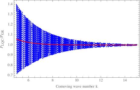
Figure 5: The ratio $\mathcal{P}^{(s,t)}_{\text{LQC}}(k)/\mathcal{P}^{(s,t)}_{\text{GR}}(k)$ between the power spectrum with the bounce effects and the standard power-law one obtained in GR. The dotted blue curve denotes the analytical power spectrum, which obviously oscillates rapidly with $k$. The solid red curve shows the average of the oscillating spectrum.

It should also be noted that the solution with the PT potential is not valid for the modes with a very small $k$ (i.e., $k\ll|a^{\prime\prime}/a|$ holds all the time during the bouncing phase). For these modes, if we ignore the $k^{2}$ term in Eq. (5), the solution can be approximated by deformed_tensor ,

$$\mu_{k}(\eta)\simeq a_{k}a(\eta)+\frac{b_{k}}{a(\eta)}.$$ (16)

However, we are not interested in these modes, as they currently are still outside of the observable universe.

Figure 6: Observational constraints for $(n_{s},k_{\text{B}}/\text{Mpc}^{-1})$ at 68% and 95% C.L. by using the Planck 2015 TT+lowP and TT, TE, EE+lowP data with $a_{0}=1$. The upper panel only considers the scalar spectrum, while the bottom includes the tensor.

IV Observational Constraints

Table 1: The Best fitting values of the six cosmological parameters and the constraints on $k_{\text{B}}/a_{0}$ and $r$ at 95% C.L for different cosmological models from different data combinations.

Parameter	Planck TT+lowP	Planck TT,TE,EE+lowP	Planck TT+lowP+$r$	Planck TT,TE,EE+lowP+$r$
$\Omega_{\rm b}h^{2}$	$0.022355$	$0.022193$	$0.022322$	$0.022064$
$\Omega_{c}h^{2}$	$0.11893$	$0.12000$	$0.11908$	$0.12071$
$100\theta_{\rm MC}$	$1.04115$	$1.04065$	$1.04080$	$1.04057$
$\tau$	$0.077835$	$0.089272$	$0.081955$	$0.085259$
$\ln(10^{10}A_{s})$	$3.088$	$3.112$	$3.101$	$3.104$
$n_{s}$	$0.9662$	$0.9647$	$0.9658$	$0.9607$
$k_{\rm B}/a_{0}$	$<3.12\times 10^{-4}$	$<3.05\times 10^{-4}$	$<3.14\times 10^{-4}$	$<3.14\times 10^{-4}$
$r$	$----$	$----$	$<0.113$	$<0.107$

The quantum corrections (14) are $k$-dependent and expected to be constrained by observations. In the following, we perform the CMB likelihood analysis by using the Planck 2015 data Planck2015 , with the MCMC code developed in cosmomc . We assume the flat cold dark matter model with the effective number of neutrinos $N_{\text{eff}}=3.046$ and choose the total neutrino mass as $\Sigma m_{\nu}=0.06{\text{eV}}$. We also write

$$\mathcal{P}_{\text{GR}}^{(s,t)}(k)=A_{(s,t)}\left(\frac{k}{k_{*}}\right)^{n^{(s,t)}_{\text{inf}}},$$ (17)

where $k_{*}(=0.05{\rm Mpc}^{-1})$ denotes the pivot scale, $n^{(s)}_{\text{inf}}=n_{s}-1$ and $n^{(t)}_{\text{inf}}=n_{t}$. We vary the seven parameters, $\Omega_{\rm b}h^{2},\Omega_{\text{c}}h^{2},\tau,\Theta_{s},n_{s},A_{s},k_{\text{B}}/a_{0}$ Zhu2 . For the six cosmological parameters except $k_{\rm B}/a_{0}$ ($\Omega_{\rm b}h^{2},\Omega_{\text{c}}h^{2},\tau,\Theta_{s},n_{s},A_{s})$, we use the same prior ranges as those adopted in Planck_parameters , while for the parameter $k_{\rm B}$ which is related to the bouncing effects, we set the prior range to $k_{\rm B}\in[10^{-8},0.002]$.

In particular, we use the high-$l$ CMB temperature power spectrum (TT) and polarization data (TT, TE, EE) respectively with the low-$l$ polarization data (lowP) from Planck2015. In Table. 1, we list the best fit values of the six cosmological parameters and constraints on $k_{\rm B}/a_{0}$ and $r$ at $95\%$ C.L. for different cosmological models from different data combinations.

Marginalizing other parameters, we find that $k_{\text{B}}/a_{0}$ is constrained by the Planck TT+lowP (Planck TT,TE,EE+lowP) to

$$\frac{k_{\text{B}}}{a_{0}}<3.12\times 10^{-4}\text{Mpc}^{-1}(3.05\times 10^{-4}),$$ (18)

at 95% C.L [cf. Fig. 6]. When we consider the ratio $r=A_{(t)}/A_{(s)}$, the Planck TT+lowP (Planck TT,TE,EE+lowP) data yields

$$\frac{k_{\text{B}}}{a_{0}}<3.14\times 10^{-4}\text{Mpc}^{-1}(3.14\times 10^{-4}),$$ (19)

at 95% C.L. These upper bounds show that the observational constraints on the bouncing effects are robust with respect to different data sets (without/with the polarization data included) and whether the tensor spectrum is included or not. In Fig. 7 we show constraints on a couple of cosmological parameters and their respective probability distributions for the CosmoMC runs described above and for the results from the Planck 2015 data. We notice that the colored curves which represent the probability distributions of $k_{\rm B}/a_{0}$ are almost perfectly superposed, which strongly indicates again that the constraints on $k_{\rm B}$ derived in this paper are robust.

Using the relation

$$\frac{k_{\text{B}}}{a_{0}}=\sqrt{\frac{\gamma_{\rm B}}{3}}\frac{a_{\rm B}}{a_{0}}m_{\rm Pl}=\sqrt{\frac{\gamma_{\rm B}}{3}}m_{\rm Pl}e^{-N_{\rm tot}},$$ (20)

where $N_{\rm tot}\equiv\ln{(a_{0}/a_{\rm B})}$ denotes the total e-folds from the quantum bounce until today, then the above upper bounds on $k_{\rm B}/a_{0}$ can be translated into the constraint on the total $e$-folds $N_{\text{tot}}$ as

$$N_{\rm tot}>141\;\;(95\%{\rm C.L.}),$$ (21)

where we have taken $\rho_{\text{c}}=0.41m_{\text{Pl}}^{4}$ planck_extension ; planck_extension_CQG . This in turn leads to a lower bound of $\delta N_{*}$,

$$\delta N_{*}>N_{\text{tot}}-N_{*}-N_{\text{after}},$$ (22)

where $\delta N_{*}\equiv\ln{(a_{*}/a_{B})}$, $N_{*}\equiv\ln{(a_{\text{end}}/a_{*})}$, and $N_{\text{after}}\equiv\ln{(a_{0}/a_{\text{end}})}$, where $a_{*}$ denotes the expansion factor at the moment that the current Horizon exited the Hubble horizon during the slow-roll inflation, and $a_{\text{end}}$ is that of the end of inflation. Taking $N_{*}\simeq 60\simeq N_{\text{after}}$, we find

$$\delta N_{*}\gtrsim 21.$$ (23)

Note that our results given by Eqs.(21) and (23) are based on three assumptions: (1) the Universe is filled with a scalar field with its potential $V(\phi)$; (2) the background evolution initially is dominated completely by the kinetic energy of the scalar field; and (3) the Universe is in the BD vacuum state in the contracting phase ($t\lesssim-t_{s}$, as shown in Fig. 2).

Figure 7: Observational constraints on a couple of parameters ($68\%$ and $95\%$ contour lines) and the probability distributions for $\ln(10^{10}A_{s})$, $n_{s}$, $k_{\rm B}/a_{0}$, and $r$ by using the Planck 2015 data. Note that in the numerical simulations we set $a_{0}=1$.

V Conclusions

In this Letter, we analytically studied the evolutions of the background and the linear scalar and tensor perturbations of the FLRW universe in LQC within the framework of the dressed metric approach (planck_extension, ; planck_extension_CQG, ; quadratic_loop, ), and showed that, if the pre-inflationary phase is dominated by the kinematic energy of the inflaton, the evolutions will be independent of the slow-roll inflationary models during this phase [cf. Fig. 1 and Eqs. (3) and (14)]. Imposing the BD vacuum in the contracting phase ($t\lesssim-t_{s}$ as shown in Fig. 2), we obtained the Bogoliubov coefficients (III) at the onset of the slow-roll inflation, which shows clearly that during the pre-inflationary phase, particles are generically created ($\left.\beta_{k}\right|_{t=t_{i}}\not=0$), and the resulting power spectra are $k$-dependent. This is in contrast to GR (where the BD vacuum ($\left.\beta_{k}\right|_{t=t_{i}}=0$) is usually imposed at the onset of the slow-roll inflation inflation . This provides a potential window to test LQC directly by the measurements of CMB and galaxy surveys (Abazajian et al., 2015). In particular, fitting the power spectra to the Planck 2015 temperature (TT+lowP) and polarization (TT,TE,EE+lowP) data, we found the lower bound for $N_{\text{tot}}\equiv\ln{(a_{0}/a_{B})}>141$ (95% C.L.). That is, to be consistent with current observations of CMB, the universe must have expanded at least 132 e-folds since the bounce.

References

- (1) A.H. Guth, Inflationary universe: A possible solution to the horizon and flatness problems, Phys. Rev. D 23, 347 (1981); A.A. Starobinsky, A new type of isotropic cosmological models without singularity, Phys. Lett. B 91, 99 (1980); K. Sato, First-order phase transition of a vacuum and the expansion of the universe, Mon. Not. R. Astron. Soc. 195, 467 (1981).
- (2) E. Komatsu et al. (WMAP Collaboration), Seven-Year Wilkinson Microwave Anisotropy Probe (WMAP) Observations: Cosmological Interpretation, Astrophys. J. Suppl. Ser. 192, 18 (2011); D. Larson et al. (WMAP Collaboration), Seven-Year Wilkinson Microwave Anisotropy Probe (WMAP) Observations: Power Spectra And Wmap - Derived Parameters, Astrophys. J. Suppl. Ser. 192, 16 (2011).
- (3) P. Ade et al. (PLANCK Collaboration), Planck 2013 results. XXII. Constraints on inflation, A&A 571, A22 (2014) [arXiv:1303.5082].
- (4) P. A. R. Ade et al. (PLANCK Collaboration), Planck 2015 results. XX. Constraints on inflation, arXiv:1502.02114.
- (5) J. Martin, C. Ringeval, and V. Vennin, Encyclopaedia Inflationaris, Phys. Dark Univ. 5 (2014) 75 [arXiv:1303.3787].
- (6) R.H. Brandenberger, Inflationary Cosmology: Progress and Problems, arXiv:hep-th/9910410; J. Martin and R.H. Brandenberger, The Trans-Planckian Problem of Inflationary Cosmology, Phys. Rev. D 63, 123501 (2001). R.H. Brandenberger and J. Martin, Trans-Planckian issues for inflationary cosmology, Class. Quantum. Grav. 30, 113001 (2013).
- (7) A. Borde and A. Vilenkin, Eternal inflation and the initial singularity, Phys. Rev. Lett. 72, 3305 (1994); A. Borde, A.H. Guth, and A. Vilenkin, Inflationary spacetimes are incomplete in past directions, Phys. Rev. Lett. 90, 151301 (2003).
- (8) D. Baumann, TASI Lectures on Inflation, arXiv:0907.5424; C.P. Burgess, M. Cicoli, F. Quevedo, String Inflation After Planck 2013, JCAP 11 (2013) 003; D. Baumann and L. McAllister, Inflation and String Theory (Cambridge Monographs on Mathematical Physics, Cambridge University Press, 2015); E. Silverstein, TASI lectures on cosmological observables and string theory, arXiv:1606.03640.
- (9) ] I. Agullo, A. Ashtekar, and W. Nelson, Quantum Gravity Extension of the Inflationary Scenario, Phys. Rev. Lett. 109, 251301 (2012); Phys. Rev. D 87, 043507 (2013).
- (10) I. Agullo, A. Ashtekar, and W. Nelson, The pre-inflationary dynamics of loop quantum cosmology: confronting quantum gravity with observations, Class. Quantum Grav. 30, 085014 (2013).
- (11) I. Agullo and N. A. Morris, Detailed analysis of the predictions of loop quantum cosmology for the primordial power spectra, Phys. Rev. D 92, 124040 (2015).
- (12) A. Ashtekar and P. Singh, Loop quantum cosmology: a status report, Class. Quantum Grav.28, 213001 (2011).
- (13) A. Ashtekar and A. Barrau, Loop quantum cosmology: from pre-inflationary dynamics to observations, Class. Quantum Grav. 32, 234001 (2015).
- (14) A. Barrau and B. Bolliet, Some conceptual issues in loop quantum cosmology, arXiv:1602.04452.
- (15) J. Yang, Y. Ding, and Y. Ma, Alternative quantization of the Hamiltonian in loop quantum cosmology, Phys. Lett. B. 682, 1 (2009).
- (16) A. Ashtekar and D. Sloan, Loop quantum cosmology and slow roll inflation, Phys. Lett. B 694, 108 (2010); Probability of inflation in loop quantum cosmology, Gen. Relativ. Gravit. 43, 3619 (2011).
- (17) P. Singh, K. Vandersloot, and G. V. Vereshchagin, Nonsingular bouncing universes in loop quantum cosmology, Phys. Rev. D 74, 043510 (2006); J. Mielczarek, T. Cailleteau, J. Grain, and A. Barrau, Inflation in loop quantum cosmology: Dynamics and spectrum of gravitational waves, Phys. Rev. D 81, 104049 (2010).
- (18) X. Zhang and Y. Ling, Inflationary universe in loop quantum cosmology, J. Cosmol. Astropart. Phys. 08, 012 (2007); L. Chen and J.-Y. Zhu, Loop quantum cosmology: The horizon problem and the probability of inflation, Phys. Rev. D 92, 084063 (2015).
- (19) B. Bolliet, J. Grain, C. Stahl, L. Linsefors, and A. Barrau, Comparison of primordial tensor power spectra from the deformed algebra and dressed metric approaches in loop quantum cosmology, Phys. Rev. D 91, 084035 (2015).
- (20) S. Schander, A. Barrau, B. Bolliet, L. Linsefors, and J. Grain, Primordial scalar power spectrum from the Euclidean bounce of loop quantum cosmology, Phys. Rev. D 93, 023531 (2016).
- (21) B. Bolliet, A. Barrau, J. Grain, and S. Schander, Observational Exclusion of a Consistent Quantum Cosmology Scenario, Phys. Rev. D 93, 124011 (2016); J. Grain, The perturbed universe in the deformed algebra approach of Loop Quantum Cosmology, Int. J. Mod. Phys. D 25, 1642003 (2016) [arXiv:1606.03271].
- (22) B. Bonga and B. Gupt, Inflation with the Starobinsky potential in Loop Quantum Cosmology, Gen. Relativ. Gravit. 48, 1 (2016); Phenomenological investigation of a quantum gravity extension of inflation with the Starobinsky potential, Phys. Rev. D 93, 063513 (2016).
- (23) J. Mielczarek, Possible observational effects of loop quantum cosmology, Phys. Rev. D81, 063503 (2010); L. Linsefors, T. Cailleteau, A. Barrau, and J. Grain, Primordial tensor power spectrum in holonomy corrected loop quantum cosmology, Phys. Rev. D 87, 107503 (2013); J. Mielczarek, Gravitational waves from the big bounce, J. Cosmol. Astropart. Phys. 11, 011 (2008).
- (24) T. Zhu, A. Wang, K. Kirsten, G. Cleaver, and Q. Sheng, High-order primordial perturbations with quantum gravitational effects, Phys. Rev. D 93, 123525 (2016).
- (25) T. Zhu, A. Wang, K. Kirsten, G. Cleaver, and Q. Sheng, in preparation (2016).
- (26) I. Agullo, W. Nelson, and A. Ashtekar, Preferred instantaneous vacuum for linear scalar fields in cosmological space-times, Phys. Rev. D 91, 064051 (2015).
- (27) E. Wilson-Ewing, Lattice loop quantum cosmology: scalar perturbations, Class. Quant. Grav. 29, 215013 (2012); The Matter Bounce Scenario in Loop Quantum Cosmology, JCAP 03, 026 (2013).
- (28) A. Lewis and S. Bridle, Cosmological parameters from CMB and other data: A Monte Carlo approach, Phys. Rev. D 66, 103511 (2002); Y.-G. Gong, Q. Wu, and A. Wang, Dark Energy and Cosmic Curvature: Monte Carlo Markov Chain Approach, Astrophys. J. 681, 27 (2008).
- (29) P. Ade et al. (PLANCK Collaboration), Planck 2013 results. XVI. Cosmological parameters, A&A 571, A16 (2014) [arXiv:1303.5076].
- (30) T. Zhu, A. Wang, G. Cleaver, K. Kirsten, Q. Sheng, and Q. Wu, DETECTING QUANTUM GRAVITATIONAL EFFECTS OF LOOP QUANTUM COSMOLOGY IN THE EARLY UNIVERSE?, Astrophys. J. Lett. 807, L17 (2015).
- Abazajian et al. (2015) K. N. Abazajian, K. Arnold, J. Austermann, B.A. Benson et al. 2015, Inflation Physics from the Cosmic Microwave Background and Large Scale Structure, Astropart. Phys. 63, 55 (2015) [ arXiv:1610.02743].