What’s in the Loop?
The Anatomy of Double Higgs Production
Abstract
Determination of Higgs self-interactions through the double Higgs production from gluon fusion is a major goal of current and future collider experiments. We point out this channel could help disentangle and resolve the nature of ultraviolet contributions to Higgs couplings to two gluons. Analytic properties of the double Higgs amplitudes near kinematic threshold are used to study features resulting from scalar and fermionic loop particles mediating the interaction. Focusing on the invariant mass spectrum, we consider the effect from anomalous top and bottom Yukawa couplings, as well as from scalar and fermionic loop particles. In particular, the spectrum at high invariant mass is sensitive to the spin of the particles in the loop.
I Introduction
Now that the Higgs boson has been discovered at GeV, the next important task is a detailed exploration of the Higgs properties. The measured Higgs boson production rates and the extracted values of the Higgs couplings are close to the Standard Model (SM) predictions, but at the level, there is room for new physics effects in the Higgs sector. The structure of the Higgs potential is completely determined in the SM and measuring the Higgs self-interactions is an important step in determining if the observed boson is identical to the Higgs boson predicted by the SM. The Higgs self-interactions are most directly probed by double Higgs () production at the Large Hadron Collider (LHC), , which has a very small rate, at TeV Plehn et al. (1996); Glover and van der Bij (1988); Dawson et al. (1998); de Florian and Mazzitelli (2013); Frederix et al. (2014); Maltoni et al. (2014); Grigo et al. (2014), making this measurement only feasible at high luminosity Moretti et al. (2005); Binoth et al. (2006); Grober and Muhlleitner (2011); Shao et al. (2013); Goertz et al. (2013); Barr et al. (2014); Barger et al. (2014); Ferreira de Lima et al. (2014); Wardrope et al. (2014); Papaefstathiou (2015); Dolan et al. (2012). In the SM the cross section receives contributions from both box and triangle diagrams, and the large cancellation between the diagrams at threshold makes the process particularly sensitive to new physics contributions Arhrib et al. (2009); Baglio et al. (2013); Dolan et al. (2013); Cao et al. (2013); Nhung et al. (2013); Han et al. (2014); Haba et al. (2014); Slawinska et al. (2014); Goertz et al. (2014); Chen and Low (2014); Li et al. (2015); Dicus et al. (2015).
Beyond-the-SM (BSM) physics can contribute to production in a variety of ways, including anomalous () and couplings Delaunay et al. (2013); Nishiwaki et al. (2014); Chen et al. (2014); Azatov et al. (2015a); Contino et al. (2012, 2010); Gillioz et al. (2012); Liu et al. (2015), resonant enhancements Christensen et al. (2013); Gouzevitch et al. (2013); Liu et al. (2013); No and Ramsey-Musolf (2014); Baglio et al. (2014); Kumar and Martin (2014); Hespel et al. (2014); Barger et al. (2015); Chen et al. (2015); van Beekveld et al. (2015), exotic decays Ellwanger and Teixeira (2014); van Beekveld et al. (2015) and new colored scalar Belyaev et al. (1999); Barrientos Bendezu and Kniehl (2001); Asakawa et al. (2010); Kribs and Martin (2012); Enkhbat (2014); Heng et al. (2014) or fermonic Liu et al. (2004); Dib et al. (2006); Pierce et al. (2007); Ma et al. (2009); Han et al. (2010); Dawson et al. (2013); Edelhaeuser et al. (2015) particles contributing to the loop amplitudes. Some of these effects, for example the modified couplings or new colored particles in the loop, also affect the single Higgs () production in the channel. However, it is difficult to disentangle new physics effects in production because of the limited number of kinematic observables in the final state. Using the higher-order process of may help with measuring the top Yukawa coupling Grojean et al. (2014); Azatov and Paul (2014), but is unlikely to resolve the nature of the colored particle mediating the loop. In this work we are interested in the question of whether production is sensitive to the underlying ultraviolet source of new physics and can potentially differentiate between different sources of new physics. We will see that many of the aforementioned new physics effects can significantly change the rate as well as the kinematic distributions in production. (See Refs. Asakawa et al. (2010); Chen and Low (2014) for previous studies of new physics effects in the kinematic distributions.) In some cases, the changes are severely restricted by the (close to SM predicted) measurements of production.
This work is organized as follows. In Section II, we review the basics of and production to set our notation. One of our major new results is in Section III, where we discuss the analytic structure of the amplitude near threshold in the case where the new physics arises from heavy fermions or from heavy colored scalars in the loops. Section IV contains numerical results for production at and TeV. The amplitude for production from intermediate colored scalar loops is reviewed in an appendix.
II Basics of and cross-sections
In this section, we review the lowest order results for and production from gluon fusion in order to fix our notation. We begin by presenting an effective Lagrangian, and then consider the specific contributions from heavy fermions and heavy colored scalars.
II.1 Non-SM Interactions
We consider the following effective Lagrangian, where we are only interested in new physics affecting Higgs rates, assume SM kinetic energy terms (), and assume no light particles other than those of the SM. Including only third generation fermions,
| (1) | |||||
where in the SM, . Global fits to Higgs production rates at the LHC limit the deviations of and from in a correlated fashion, as described below in Eq. 11. Deviations of the -Yukawa coupling from the SM prediction, , are less constrained collaboration (2015); Khachatryan et al. (2014a).
II.2 Colored scalars
The contributions from colored scalars depend on the parameters of the scalar potential. We use the following Lagrangian for an singlet, complex scalar, ,
| (2) | |||||
| (3) |
where is the SM doublet with . In this normalization, the Fermi constant and GeV. If the scalar, , is real,
| (4) |
The physical mass for either a real or complex scalar is,
| (5) |
where is the limit where the scalar gets all of its mass from electroweak symmetry breaking. The cubic and quartic scalar couplings are,
| (6) |
and similarly for a real scalar.
II.3 Production from Scalars and Fermions
The leading-order (LO) production rates due to virtual scalars and fermions are well-known. It is convenient to introduce the loop functions
| (7) | |||||
| (8) |
where and
| (9) | |||||
Then including colored scalars and non-SM fermion interactions as defined in the previous subsections,
| (10) | |||||
where is the Dynkin index for the corresponding representation under defined as , and for real scalars and 1 for complex scalars. The Dynkin index is for fundamental representations and for adjoint representations, respectively. For SM fermions, .
Neglecting the -quark contribution and noting that and are well approximated by their large mass limits, and ,
| (11) | |||||
Eq. 11 is the well-known result that production has little discriminating power between and Banfi et al. (2014); Dawson et al. (2014); Azatov et al. (2015b, 2014). The coefficients of and from heavy colored scalars can be found in Refs. Dawson et al. (2015); Bonciani et al. (2007); Gori and Low (2013). In the SM, production receives significant QCD corrections beyond LO QCD. The NNLO contributions from arbitrary fermions Anastasiou et al. (2010) and scalars Boughezal (2011); Boughezal and Petriello (2010) are significant. However, since we are typically concerned with ratios relative to the SM, we work at leading order.
II.4 Production for Fermions and Scalars


The LO production rates from fermion and scalar loops can be found in Refs. Glover and van der Bij (1988); Plehn et al. (1996) and Refs. Asakawa et al. (2010); Kribs and Martin (2012), respectively. The LO partonic cross-section for is given by
| (12) |
where . In the above comes from averaging over the initial gluon helicities, from color averaging and from the identical final state particles. The amplitude-squared can be written as
| (13) | |||||
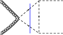
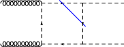
where comes from summing over the gluon color index. The form factors , , and resulting from the SM top quark are given in the appendix of Ref. Plehn et al. (1996)111 In the SM, including only the top quark contribution Eq. 13 differs from Eq. 13 in Ref. Plehn et al. (1996) as well as Eq. 4 in Ref. Baglio et al. (2013), but agrees with Eq. 6 in Ref. Glover and van der Bij (1988), Eq. 5 in Ref. Dawson et al. (2013) and Eq. 4 in Chen and Low (2014), after plugging in and taking account differences in the normalization of the form factors employed.. The Feynman diagrams for the case of scalar particles are shown in Fig. 1, and the corresponding form factors are given in Appendix A222 We disagree with the overall normalization of the corresponding expressions in Refs. Asakawa et al. (2010); Kribs and Martin (2012). In addition, the first arguments of the last function in Eq. 16 of Ref. Kribs and Martin (2012) should be swapped.. In the large mass limits,
| (14) |
In the large mass limit, only the the spin-0 contribution survives,
| (15) | |||||
The contributions from the anomalous couplings in Eq. 15 are consistent with those in Refs. Gillioz et al. (2012); Delaunay et al. (2013); Chen et al. (2014); Chen and Low (2014). Furthermore, the contributions to Eq. 15 which come from the triangle diagrams are related to the fermionic and scalar contributions to the 1-loop QCD function via the Higgs low-energy theorems Shifman et al. (1979), which can be used to systematically compute higher order QCD corrections to the triangle loops Dawson et al. (1996); Gori and Low (2013).
III Analytic Structure
A closed-form analytic expression for the production amplitude at threshold, , may be obtained from the imaginary part of the amplitude, combined with a knowledge of the amplitude’s limiting behavior as the particle masses in the loops go to either zero or infinity Li and Voloshin (2014). Alternatively, the threshold result can be obtained by a direct expansion of the full amplitude. For a colored fermion of mass running in the loops, the separate components of the amplitude arising from the triangle and box diagrams are, at threshold,
where and is again the Dynkin index of the representation of the fermion. The total amplitude is proportional to the sum of the two expressions above,
| (17) |
In the heavy mass limit,
| (18) |
and agrees with the result of Li and Voloshin (2014).
For a scalar of mass with , the triangle and box amplitudes at threshold are found by analytic continuation of the imaginary contributions given in Appendix B,
where and is the Dynkin index of the scalar’s representation. We have included bubble diagrams with quartic scalar-gluon couplings in and triangle diagrams with such couplings in . Just as for fermions, we may expand the total threshold amplitude as
| (20) |
where the functions are the threshold values of the form factors in Eq. 15. In the heavy mass limit, the threshold result is
| (21) |

The cancellations between the triangle and box functions for fermions and scalars are shown in Fig. 2. In each panel, the cancellation clearly gets more exact for heavy loop particles. However, due to the small coefficients in the expansions above, the amplitude at threshold is still significantly suppressed for finite masses. For the SM top, the indicated point in the left panel of Fig. 2 shows that the triangle and box functions cancel to . This cancellation will be spoiled by a non-SM Higgs self-coupling, additional interactions between the fermions and the Higgs boson, or if the scalar mass receives a contribution that is not from the Higgs ().
Having established that the cancellation between and is largely present for finite loop particle masses, we now investigate the behavior of the cancellation in the presence of additional couplings. It is natural to begin by considering the effect of a non-SM Higgs self-coupling on the amplitude from top loops at threshold. Such a rescaling would affect only, since the box diagrams do not involve the Higgs self-coupling. Fig. 3 shows how a modified Higgs tri-linear coupling would significantly alter the threshold amplitude, leading to the well-known result that production is a sensitive probe of the Higgs self-coupling. Indeed, for arbitrary loop particle mass, there is a perfect cancellation between the one-loop triangle and box diagrams for
| (22) |
where the ratio of the box and triangle diagrams at threshold approaches -1 as the loop particle gets infinitely heavy. For the SM top mass, the cancellation is perfect when . The next section considers further new couplings between the SM quarks and the Higgs bosons.

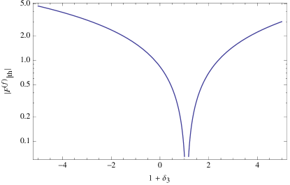
We now turn to the scalar case, including arbitrary soft masses of scalars coupling to the Higgs. For a scalar which does not receive its mass entirely from electroweak symmetry breaking, , the amplitude at threshold is
| (23) |
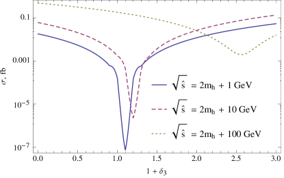
Fig. 4 shows how the cancellation between and breaks down for . We see in the left panel that the triangle and box functions do not cancel when the scalar has a soft mass term, and the total amplitude at threshold tends to a non-zero value in the limit of infinitely heavy scalar mass. The right panel shows how sensitive the cancellation between and is to the presence of soft scalar mass terms, for a selection of fixed physical scalar masses. In addition to the cancellation at , the amplitude obviously vanishes when the scalar does not couple to the Higgs, . Discounting this trivial case, the amplitude quickly grows as we move away from the scenario where the scalar gets all of its mass from the Higgs.
Finally, we examine the cancellation away from threshold. In addition to the spin- 0 amplitudes realizing their full functional dependence on the partonic CM energy beyond , there are spin-2 contributions to production. The full amplitudes are known in terms of loop integrals, and reveal the strong cancellation near threshold when evaluated numerically. In the fermion case, Fig. 5 shows how the partonic cross section changes above threshold for the SM top. Near threshold, there is a pronounced cancellation between the triangle and box diagrams for the value of the Higgs self-coupling predicted by Eq. 22. This dip shifts and becomes much weaker as we move above threshold.

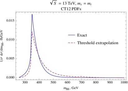

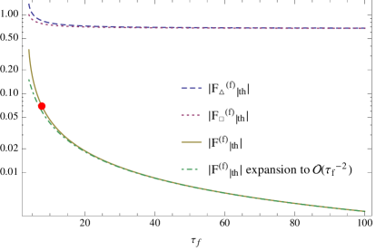
It is interesting to consider how well our closed form expressions for the threshold amplitudes approximate the full amplitudes. In the threshold amplitudes above, the Higgs mass may be considered as a proxy for the CM energy, , except in the triangle diagram where it appears in an -channel propagator. This motivates the closed form approximation,
| (24) |
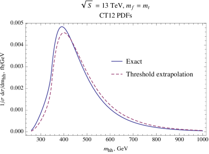
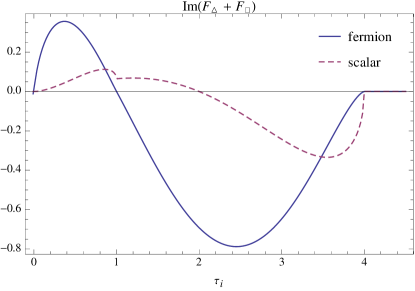
for the amplitude beyond threshold. Fig. 6 shows the result of using this approximation in Eq. 15 for loop fermions and scalars of various masses. While the total cross section predicted by the expression in Eq. 24 is not close to the true cross section, the normalized invariant mass distribution is fairly well reproduced. In particular, for , two different loop particle propagators may go on shell, causing a nonzero imaginary piece of the exact amplitude that is visible as a feature in the invariant mass distribution. Similarly, the threshold approximation in Eq. 24 includes a term proportional to . We note that there is in principle also a discontinuity in the invariant mass distribution at , captured by terms proportional to in the threshold approximation. However, there is no visible corresponding feature in the invariant mass distributions of Fig. 6. The discontinuities at and correspond to the discontinuities in the threshold amplitudes at and , respectively. Fig. 7 shows the imaginary parts of the threshold amplitudes, allowing us to compare the discontinuities. The unphysical discontinuity at , which may be traced back to the terms in the threshold amplitudes of Eqs. III and III, is not shown. For both fermions Li and Voloshin (2014) and scalars, we observe a much larger discontinuity at than at , due to the lack of any imaginary piece of the amplitude for . The much smaller discontinuities in the imaginary part of the threshold amplitudes explain the lack of any visible features at .
IV Examples
The previous section demonstrated how the threshold cancellations between triangle and box diagrams render production extremely sensitive to non-SM couplings. In this section we consider modifications of the distributions from anomalous fermionic Yukawa couplings, from colored scalar loops, and from fermionic top partners. Effects of anomalous couplings on the kinematic distributions have been examined in Chen and Low (2014). In some cases the allowed new interactions are severely restricted by the requirement that production occur at the observed rate. In addition, we are interested in whether production distributions can distinguish between fermion and scalar loop contributions.
In all of our numerical results we use CT12 NLO PDFs Owens et al. (2013); Gao et al. (2014) with the associated NLO values for , and take GeV, GeV, and GeV. For production we take , while for production we set . We use the LO -loop predictions for both and production. In addition, the 1-loop functions are evaluated using the software LoopTools Hahn and Perez-Victoria (1999), as well as independent in-house routines.
IV.1 Anomalous Yukawa Couplings
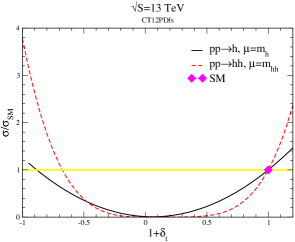
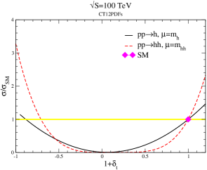
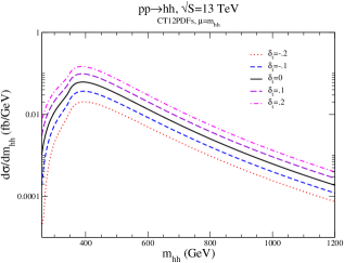
We begin by considering the effects of anomalous top Yukawa couplings in Eq. 1, assuming all other couplings are SM-like. In Fig. 8, we show the both the and rates, normalized to the one-loop SM rate as a function of the top quark Yukawa. For positive , the requirement that only allows a deviation in .333We note that negative is now excluded by global fits to Higgs couplings Khachatryan et al. (2014a); collaboration (2015). As measurements of the rate become more precise, the allowed deviations for the rate due to an anomalous top Yukawa coupling will also become smaller. An important assumption throughout this work is that there are no light particles which could allow for resonant production of two Higgs bosons, in which case the spectrum would exhibit a clear peak at the mass of the resonance. The effect of a non-SM top Yukawa coupling on the invariant mass distribution is shown in Fig. 9 for both and TeV.444There is not much difference in the invariant mass spectra between and 100 TeV. This feature has also been observed in Ref. Chen and Low (2014). When , the cancellation between box and triangle diagrams described in the previous section is spoiled and the resulting cross sections vary by up to a factor of two Baur et al. (2002, 2003). This same variation is seen at both TeV and TeV. The effect of changing the top Yukawa coupling and the tri-linear Higgs coupling in a correlated manner can be quite dramatic, as shown in Fig. 10. Note the interesting cancellation for large and positive .


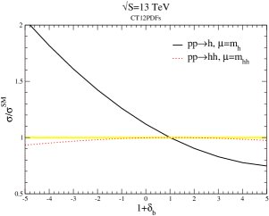
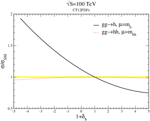
In the SM, the contribution of the quark is small for both the and production Anastasiou et al. (2011), although for large enough the production from quark initial states becomes important Dicus and Willenbrock (1989); Dawson et al. (2007). As the quark Yukawa is increased, the rate for is substantially altered, while the rate is rather insensitive to the Yukawa as seen in Fig. 11. Note that and the LHC experiments limit the total Higgs widthAad et al. (2015); Khachatryan et al. (2014b), , so this implies a rough limit .
IV.2 Fermionic Top Partners
In this subsection and the following, we consider fermion and scalar contributions to and pose the question:
-
•
Can we determine the nature of the loop particle, by examining the properties of the scattering amplitude?
We use the analytic properties of the amplitude discussed in Sec. III to draw some conclusions.

We begin by considering the effects of a heavy color triplet fermion, with mass , with a SM-like Yukawa coupling to the Higgs boson. The invariant mass distribution for this heavy fermion is compared with that from GeV in Fig. 12. The distribution has an interesting dip near due to the presence of a cut in the amplitude. This dip persists even when the Higgs tri-linear coupling is allowed to have a non-SM value, . At TeV, the invariant mass spectrum has a more significant support at large , compared to that at TeV.
A 4th generation of chiral fermions would increase the rate for production by roughly a factor of above the SM prediction, far above the allowed region from current data Khachatryan et al. (2014a); collaboration (2015). So we consider the addition of a vector-like fermonic top partner. In the simplest example, a top partner singlet model, there exists a charge- singlet particle, , which mixes with the SM-like top quark, . The Yukawa couplings in the top partner sector are Aguilar-Saavedra (2003); Dawson and Furlan (2012); Aguilar-Saavedra et al. (2013),
| (25) |
where the Standard Model-like particles are denoted as
| (26) |
The addition of the Dirac fermion mass term in Eq. 25 means that the fermion masses are not completely determined by electroweak symmetry breaking. We can always rotate such that and so there are 3 independent parameters in the top sector, which we take to be the physical charge- quark masses, and , along with the mixing angle, . In the following, we will abbreviate , . The couplings of the physical heavy charge- quarks to the Higgs boson are,
| (27) |
The parameters of the fermonic top partner model are limited by electroweak precision measurements to Aguilar-Saavedra (2003); Dawson and Furlan (2012); Aguilar-Saavedra et al. (2013) and by direct search experiments to GeV Chatrchyan et al. (2014); Aad et al. (2013).
In the limit, single Higgs production in the top partner model is virtually identical to that in the SM Azatov and Galloway (2012); Dawson and Furlan (2012); Low et al. (2010),555This is simply a statement of the decoupling limit.
| (28) |
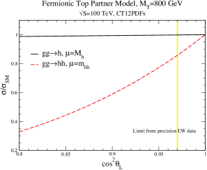
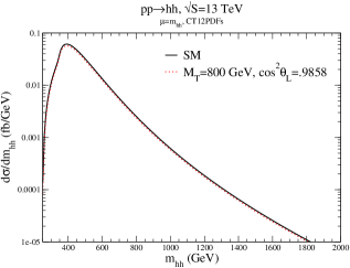
In Fig. 13, we compare the rate for and production in the singlet top partner model with GeV, as a function of the mixing angle, . For values of allowed by precision EW measurements, the rate can be seen to be indistinguishable from that of the SM. On the other hand, production receives contributions from the mixed couplings of Eq. 27 and in general can be quite different from the SM prediction, as shown in Fig. 13. Even imposing the restrictions from precision EW data, production can be reduced by up to from the SM prediction Chatrchyan et al. (2014); Aad et al. (2013), although the rate cannot be increased in this class of model. The relative reduction of the rate is roughly the same at TeV and TeV. The invariant mass spectrum are shown in Fig. 14 for the top partner model. Because the EW precision constraints require that the mixing angle be very small, the distribution in indistinguishable from that of the SM. It would be interesting to investigate slightly less simple models by including and couplings, which arise in models where the Higgs arise as a pseudo-Nambu-Goldstone boson Cheng et al. (2006); Low et al. (2010).


IV.3 Scalar Top Partners
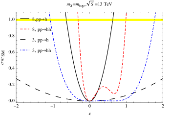
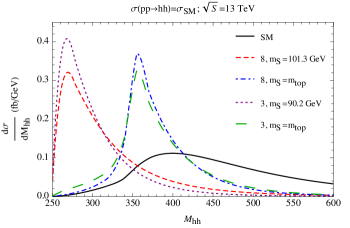
In this section, we compare the results of the previous section where the loop particles are fermions with distributions where instead of a fermion, there is a colored scalar in the loops. We begin by replacing the SM top quark in the triangle diagram and in the triangle and box diagrams with a color triplet scalar of the same mass, GeV. Fig. 15 shows the ratio of the total cross sections for both and production, normalized to the lowest order SM predictions, in this scenario. In the case of a color triplet scalar of mass GeV in the loops, we see that, in order to reproduce the SM rate for production (the black dashed line), need to be quite large, . If is tuned to obtain for , then a color octet intermediate particle replacing the top quark with positive (the solid black line) would predict a highly suppressed rate for production (the red dashed line). Alternatively, we can tune both and the scalar mass such that both and production have the SM rates, as shown in Fig. 16. Although the total rates are identical to the SM predictions, the kinematic distributions from color octet and triplet intermediate states are quite different than those from the SM top, as plotted in Fig. 17. The scalar needs to be quite light to reproduce the SM rates, and the distribution is peaked at much lower than the SM prediction.

We also consider Higgs production in the presence of the SM top quark and a colored scalar666In supersymmetry there are two colored scalars, the top squarks, mediating in the loop. Such a possibility is beyond the scope of current work and will be pursued elsewhere Dawson et al. .. Assuming the top Yukawa is SM-like, an additional scalar receiving all of its mass from electroweak symmetry breaking would give an unacceptably large contribution to the production cross section, regardless of its mass and representation. This immediately follows from Eq. 10: A heavy color triplet scalar with changes the production rate by 54%. Lighter scalars and scalars in other color representations result in even larger deviations. Fig. 18 shows the effects of color triplet and octet scalars on production in the large mass limit, as functions of the proportion of the scalar mass coming from the Higgs field. Heavy scalars receiving all their masses from the Higgs have , and are not compatible with a simple average of current ATLAS collaboration (2015) and CMS Khachatryan et al. (2014a) limits on the production rate from gluon fusion, which is drawn as a shaded band in Fig. 18.

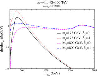
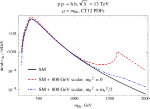
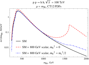
The limits imposed from production constrains the sensitivity of measurements to reveal new scalars, especially those with masses close to the weak scale. This is because a light scalar, in addition to the SM top, modifies the rate significantly, unless its coupling to the Higgs is small, which at the same time diminishes its impact in kinematic distributions. However, heavy scalars will decouple quickly in the rate and may show up in the high tail of the distribution. The invariant mass distributions for production are shown in Fig. 19 assuming a SM-like top quark and an additional 800 GeV color triplet scalar. If the scalar receives half of its mass squared from electroweak symmetry breaking, , the rate is in roughly tension with the current measurement, and the distribution deviates from the SM expectation starting at , roughly speaking. For comparison, if the entire mass of the scalar was due to the Higgs, the feature at would be quite significant.
V Conclusion
The observation of double Higgs production will be an important milestone in understanding the nature of electroweak symmetry breaking. In the past the focus of this channel has been on extracting the Higgs tri-linear self-coupling. In this work we showed that the goal can be much broader and encompass understanding the nature of the UV physics giving rise to Higgs coupling to two gluons, which is otherwise difficult to probe in single Higgs production.
In Section III, we examined the differences in the threshold behavior of double Higgs production resulting from intermediate scalar and fermion loops and in Section IV, we demonstrated that even if the parameters in a model with colored scalars are tuned to reproduce the SM rates for single and double Higgs production, the resulting invariant mass distributions can be significantly different from the SM. These distributions are also very sensitive to whether an additional scalar gets all of its mass from electroweak symmetry breaking. While Higgs plus jet production is also sensitive to the spin of loop particles and has a greater cross section, it does not enjoy the same large amplitude cancellation present in double Higgs production Bonciani et al. (2007). We also investigated the effects of anomalous top and bottom Yukawa couplings and showed that the resulting changes in single and double Higgs production relative to the SM rates are roughly the same at and TeV.
Clearly, it will be an important experimental question on how to extract the wealth of information contained in the double Higgs production. Our work provides strong motivation to pursue this issue experimentally.
Acknowledgements.
We thank A. Martin for useful discussions of Ref. Kribs and Martin (2012). A.I. acknowledges R. Boughezal and F. Petriello for discussions. The work of S.D. is supported by the U.S. Department of Energy under grant No. DE-AC02-98CH10886. Work at ANL is supported by the U.S. Department of Energy under grant No. DE-AC02-06CH11357. A.I. is supported in part by the U.S. Department of Energy under grant DE-FG02-12ER41811. I.L. is supported in part by the U.S. Department of Energy under grant No. DE-SC0010143.Appendix A Amplitudes from scalars
Appendix B Closed Form Amplitudes for
Here, we calculate the imaginary part of the amplitude for production from scalar loops at threshold, using cut techniques. This is a new result analogous to the recent computation for fermions Li and Voloshin (2014). By using the dispersion relation, we may recover the full amplitude in closed form, which is then analyzed in Section III.
We start with the general amplitude in Eq. 15. For simplicity, we assume a single scalar that gets all of its mass from the Higgs, so that and in Eq. 3. Our results can easily be generalized to scalars with arbitrary couplings and masses, and we emphasize that they do not assume a heavy loop particle. At threshold, , only the spin 0 piece contributes Dawson et al. (2013). The imaginary parts of the corresponding form factors can be obtained from cutting all possible diagrams, and sending all cut propagators on shell. We will compute and separately at threshold.


Fig. 20 shows the diagrams that are responsible for the form factor. In addition to the triangle diagram which may be obtained by replacing the top quark in the SM double Higgs triangle diagram with a scalar, we have the additional coupling. We also include bubble diagrams with quartic scalar-gluon couplings with the above diagrams in the triangle form factors, as they are related through gauge invariance. Now, the imaginary part of the double Higgs amplitude receives contributions from the cuts shown in the diagrams of Fig. 20, through
| (B.1) |
where , and refer to the full double Higgs amplitude and the left/right halves of a cut diagram. The integral is over the phase space of the cut propagators. Each cut diagram in Fig. 20 contributes separately to . The halves of the cut diagrams are simply tree-level amplitudes for and . Furthermore, since we are interested in the amplitude cancellation at threshold, we may project out the spin 0 piece of the amplitude to get . The kinematics of Appendix A simplify considerably for , and we are left with
| (B.2) |


Cut diagrams that contribute to and are shown in Fig. 21. The first two diagrams of Fig. 21 have identical cuts to the diagrams of Fig. 20, and the left sides are the same as in the earlier diagrams. At threshold with the cut propagators on shell, comparison of the right sides of these diagrams with those of Fig. 20 immediately gives
| (B.3) |
This is the contribution of the top row of Fig. 21 to .
The contributions of the cuts in the third and fourth diagrams of Fig. 21 to at threshold may be computed from the tree-level amplitudes for and . Note that the two adjacent propagators attaching to either external Higgs may be cut, each choice leading to an identical set of contributions to the imaginary amplitude. Only one such set of cuts is shown in these diagrams. Both sets of cuts together yield
| (B.4) |
Also, there is no contribution to the imaginary part of the amplitude from cutting two adjacent propagators attaching to an external gluon, because the amplitude for is zero when the scalars are put on shell.
Finally, the last cut diagram of Fig. 21 gives a contribution to that may be calculated at threshold from the amplitude. We proceed as before, and find the final contribution
| (B.5) |
The sum of the right-hand sides of Eqs. B.2, B.3, B.4 and B.5 gives the full imaginary amplitude at threshold. Now, we turn to the limits of the full amplitude as . In the limit , the amplitude vanishes since for a scalar that gets all its mass from the Higgs, is proportional to through
| (B.6) |
On the other hand, in the infinite scalar mass limit we may apply the low-energy theorem. From the effective Lagrangian for the interaction between scalars and gluons Shifman et al. (1979), we know that the amplitude goes as
| (B.7) | |||||
which vanishes for the SM Higgs self-coupling Li and Voloshin (2014). Given the limiting behavior of the amplitude combined with full knowledge of its imaginary part, then, the dispersion relation gives the full amplitude in Eq. III.
References
- Plehn et al. (1996) T. Plehn, M. Spira, and P. Zerwas, Nucl.Phys. B479, 46 (1996), eprint hep-ph/9603205.
- Glover and van der Bij (1988) E. N. Glover and J. van der Bij, Nucl.Phys. B309, 282 (1988).
- Dawson et al. (1998) S. Dawson, S. Dittmaier, and M. Spira, Phys.Rev. D58, 115012 (1998), eprint hep-ph/9805244.
- de Florian and Mazzitelli (2013) D. de Florian and J. Mazzitelli, Phys.Rev.Lett. 111, 201801 (2013), eprint 1309.6594.
- Frederix et al. (2014) R. Frederix, S. Frixione, V. Hirschi, F. Maltoni, O. Mattelaer, et al., Phys.Lett. B732, 142 (2014), eprint 1401.7340.
- Maltoni et al. (2014) F. Maltoni, E. Vryonidou, and M. Zaro, JHEP 1411, 079 (2014), eprint 1408.6542.
- Grigo et al. (2014) J. Grigo, K. Melnikov, and M. Steinhauser, Nucl.Phys. B888, 17 (2014), eprint 1408.2422.
- Moretti et al. (2005) M. Moretti, S. Moretti, F. Piccinini, R. Pittau, and A. Polosa, JHEP 0502, 024 (2005), eprint hep-ph/0410334.
- Binoth et al. (2006) T. Binoth, S. Karg, N. Kauer, and R. Ruckl, Phys.Rev. D74, 113008 (2006), eprint hep-ph/0608057.
- Grober and Muhlleitner (2011) R. Grober and M. Muhlleitner, JHEP 1106, 020 (2011), eprint 1012.1562.
- Shao et al. (2013) D. Y. Shao, C. S. Li, H. T. Li, and J. Wang, JHEP 1307, 169 (2013), eprint 1301.1245.
- Goertz et al. (2013) F. Goertz, A. Papaefstathiou, L. L. Yang, and J. Zurita, JHEP 1306, 016 (2013), eprint 1301.3492.
- Barr et al. (2014) A. J. Barr, M. J. Dolan, C. Englert, and M. Spannowsky, Phys.Lett. B728, 308 (2014), eprint 1309.6318.
- Barger et al. (2014) V. Barger, L. L. Everett, C. Jackson, and G. Shaughnessy, Phys.Lett. B728, 433 (2014), eprint 1311.2931.
- Ferreira de Lima et al. (2014) D. E. Ferreira de Lima, A. Papaefstathiou, and M. Spannowsky, JHEP 1408, 030 (2014), eprint 1404.7139.
- Wardrope et al. (2014) D. Wardrope, E. Jansen, N. Konstantinidis, B. Cooper, R. Falla, et al. (2014), eprint 1410.2794.
- Papaefstathiou (2015) A. Papaefstathiou (2015), eprint 1504.04621.
- Dolan et al. (2012) M. J. Dolan, C. Englert, and M. Spannowsky, JHEP 1210, 112 (2012), eprint 1206.5001.
- Arhrib et al. (2009) A. Arhrib, R. Benbrik, C.-H. Chen, R. Guedes, and R. Santos, JHEP 0908, 035 (2009), eprint 0906.0387.
- Baglio et al. (2013) J. Baglio, A. Djouadi, R. Gr ber, M. M hlleitner, J. Quevillon, et al., JHEP 1304, 151 (2013), eprint 1212.5581.
- Dolan et al. (2013) M. J. Dolan, C. Englert, and M. Spannowsky, Phys.Rev. D87, 055002 (2013), eprint 1210.8166.
- Cao et al. (2013) J. Cao, Z. Heng, L. Shang, P. Wan, and J. M. Yang, JHEP 1304, 134 (2013), eprint 1301.6437.
- Nhung et al. (2013) D. T. Nhung, M. Muhlleitner, J. Streicher, and K. Walz, JHEP 1311, 181 (2013), eprint 1306.3926.
- Han et al. (2014) C. Han, X. Ji, L. Wu, P. Wu, and J. M. Yang, JHEP 1404, 003 (2014), eprint 1307.3790.
- Haba et al. (2014) N. Haba, K. Kaneta, Y. Mimura, and E. Tsedenbaljir, Phys.Rev. D89, 015018 (2014), eprint 1311.0067.
- Slawinska et al. (2014) M. Slawinska, W. van den Wollenberg, B. van Eijk, and S. Bentvelsen (2014), eprint 1408.5010.
- Goertz et al. (2014) F. Goertz, A. Papaefstathiou, L. L. Yang, and J. Zurita (2014), eprint 1410.3471.
- Chen and Low (2014) C.-R. Chen and I. Low, Phys.Rev. D90, 013018 (2014), eprint 1405.7040.
- Li et al. (2015) Q. Li, Z. Li, Q.-S. Yan, and X. Zhao (2015), eprint 1503.07611.
- Dicus et al. (2015) D. A. Dicus, C. Kao, and W. W. Repko (2015), eprint 1504.02334.
- Delaunay et al. (2013) C. Delaunay, C. Grojean, and G. Perez, JHEP 1309, 090 (2013), eprint 1303.5701.
- Nishiwaki et al. (2014) K. Nishiwaki, S. Niyogi, and A. Shivaji, JHEP 1404, 011 (2014), eprint 1309.6907.
- Chen et al. (2014) C.-Y. Chen, S. Dawson, and I. Lewis, Phys.Rev. D90, 035016 (2014), eprint 1406.3349.
- Azatov et al. (2015a) A. Azatov, R. Contino, G. Panico, and M. Son (2015a), eprint 1502.00539.
- Contino et al. (2012) R. Contino, M. Ghezzi, M. Moretti, G. Panico, F. Piccinini, et al., JHEP 1208, 154 (2012), eprint 1205.5444.
- Contino et al. (2010) R. Contino, C. Grojean, M. Moretti, F. Piccinini, and R. Rattazzi, JHEP 1005, 089 (2010), eprint 1002.1011.
- Gillioz et al. (2012) M. Gillioz, R. Grober, C. Grojean, M. Muhlleitner, and E. Salvioni, JHEP 1210, 004 (2012), eprint 1206.7120.
- Liu et al. (2015) N. Liu, S. Hu, B. Yang, and J. Han, JHEP 1501, 008 (2015), eprint 1408.4191.
- Christensen et al. (2013) N. D. Christensen, T. Han, Z. Liu, and S. Su, JHEP 1308, 019 (2013), eprint 1303.2113.
- Gouzevitch et al. (2013) M. Gouzevitch, A. Oliveira, J. Rojo, R. Rosenfeld, G. P. Salam, et al., JHEP 1307, 148 (2013), eprint 1303.6636.
- Liu et al. (2013) J. Liu, X.-P. Wang, and S.-h. Zhu (2013), eprint 1310.3634.
- No and Ramsey-Musolf (2014) J. M. No and M. Ramsey-Musolf, Phys.Rev. D89, 095031 (2014), eprint 1310.6035.
- Baglio et al. (2014) J. Baglio, O. Eberhardt, U. Nierste, and M. Wiebusch, Phys.Rev. D90, 015008 (2014), eprint 1403.1264.
- Kumar and Martin (2014) N. Kumar and S. P. Martin, Phys.Rev. D90, 055007 (2014), eprint 1404.0996.
- Hespel et al. (2014) B. Hespel, D. Lopez-Val, and E. Vryonidou, JHEP 1409, 124 (2014), eprint 1407.0281.
- Barger et al. (2015) V. Barger, L. L. Everett, C. Jackson, A. D. Peterson, and G. Shaughnessy, Phys.Rev.Lett. 114, 011801 (2015), eprint 1408.0003.
- Chen et al. (2015) C.-Y. Chen, S. Dawson, and I. Lewis, Phys.Rev. D91, 035015 (2015), eprint 1410.5488.
- van Beekveld et al. (2015) M. van Beekveld, W. Beenakker, S. Caron, R. Castelijn, M. Lanfermann, et al. (2015), eprint 1501.02145.
- Ellwanger and Teixeira (2014) U. Ellwanger and A. M. Teixeira (2014), eprint 1412.6394.
- Belyaev et al. (1999) A. Belyaev, M. Drees, O. J. Eboli, J. Mizukoshi, and S. Novaes, Phys.Rev. D60, 075008 (1999), eprint hep-ph/9905266.
- Barrientos Bendezu and Kniehl (2001) A. Barrientos Bendezu and B. A. Kniehl, Phys.Rev. D64, 035006 (2001), eprint hep-ph/0103018.
- Asakawa et al. (2010) E. Asakawa, D. Harada, S. Kanemura, Y. Okada, and K. Tsumura, Phys.Rev. D82, 115002 (2010), eprint 1009.4670.
- Kribs and Martin (2012) G. D. Kribs and A. Martin, Phys.Rev. D86, 095023 (2012), eprint 1207.4496.
- Enkhbat (2014) T. Enkhbat, JHEP 1401, 158 (2014), eprint 1311.4445.
- Heng et al. (2014) Z. Heng, L. Shang, Y. Zhang, and J. Zhu, JHEP 1402, 083 (2014), eprint 1312.4260.
- Liu et al. (2004) J.-J. Liu, W.-G. Ma, G. Li, R.-Y. Zhang, and H.-S. Hou, Phys.Rev. D70, 015001 (2004), eprint hep-ph/0404171.
- Dib et al. (2006) C. O. Dib, R. Rosenfeld, and A. Zerwekh, JHEP 0605, 074 (2006), eprint hep-ph/0509179.
- Pierce et al. (2007) A. Pierce, J. Thaler, and L.-T. Wang, JHEP 0705, 070 (2007), eprint hep-ph/0609049.
- Ma et al. (2009) W. Ma, C.-X. Yue, and Y.-Z. Wang, Phys.Rev. D79, 095010 (2009), eprint 0905.0597.
- Han et al. (2010) X.-F. Han, L. Wang, and J. M. Yang, Nucl.Phys. B825, 222 (2010), eprint 0908.1827.
- Dawson et al. (2013) S. Dawson, E. Furlan, and I. Lewis, Phys.Rev. D87, 014007 (2013), eprint 1210.6663.
- Edelhaeuser et al. (2015) L. Edelhaeuser, A. Knochel, and T. Steeger (2015), eprint 1503.05078.
- Grojean et al. (2014) C. Grojean, E. Salvioni, M. Schlaffer, and A. Weiler, JHEP 1405, 022 (2014), eprint 1312.3317.
- Azatov and Paul (2014) A. Azatov and A. Paul, JHEP 1401, 014 (2014), eprint 1309.5273.
- collaboration (2015) T. A. collaboration (2015).
- Khachatryan et al. (2014a) V. Khachatryan et al. (CMS) (2014a), eprint 1412.8662.
- Banfi et al. (2014) A. Banfi, A. Martin, and V. Sanz, JHEP 1408, 053 (2014), eprint 1308.4771.
- Dawson et al. (2014) S. Dawson, I. Lewis, and M. Zeng, Phys.Rev. D90, 093007 (2014), eprint 1409.6299.
- Azatov et al. (2015b) A. Azatov, C. Grojean, A. Paul, and E. Salvioni, Zh.Eksp.Teor.Fiz. 147, 410 (2015b), eprint 1406.6338.
- Azatov et al. (2014) A. Azatov, M. Salvarezza, M. Son, and M. Spannowsky, Phys.Rev. D89, 075001 (2014), eprint 1308.6601.
- Dawson et al. (2015) S. Dawson, I. Lewis, and M. Zeng, Phys.Rev. D91, 074012 (2015), eprint 1501.04103.
- Bonciani et al. (2007) R. Bonciani, G. Degrassi, and A. Vicini, JHEP 0711, 095 (2007), eprint 0709.4227.
- Gori and Low (2013) S. Gori and I. Low, JHEP 1309, 151 (2013), eprint 1307.0496.
- Anastasiou et al. (2010) C. Anastasiou, R. Boughezal, and E. Furlan, JHEP 1006, 101 (2010), eprint 1003.4677.
- Boughezal (2011) R. Boughezal, Phys.Rev. D83, 093003 (2011), eprint 1101.3769.
- Boughezal and Petriello (2010) R. Boughezal and F. Petriello, Phys.Rev. D81, 114033 (2010), eprint 1003.2046.
- Shifman et al. (1979) M. A. Shifman, A. Vainshtein, M. Voloshin, and V. I. Zakharov, Sov.J.Nucl.Phys. 30, 711 (1979).
- Dawson et al. (1996) S. Dawson, A. Djouadi, and M. Spira, Phys.Rev.Lett. 77, 16 (1996), eprint hep-ph/9603423.
- Li and Voloshin (2014) X. Li and M. Voloshin, Phys.Rev. D89, 013012 (2014), eprint 1311.5156.
- Owens et al. (2013) J. Owens, A. Accardi, and W. Melnitchouk, Phys.Rev. D87, 094012 (2013), eprint 1212.1702.
- Gao et al. (2014) J. Gao, M. Guzzi, J. Huston, H.-L. Lai, Z. Li, et al., Phys.Rev. D89, 033009 (2014), eprint 1302.6246.
- Hahn and Perez-Victoria (1999) T. Hahn and M. Perez-Victoria, Comput.Phys.Commun. 118, 153 (1999), eprint hep-ph/9807565.
- Baur et al. (2002) U. Baur, T. Plehn, and D. L. Rainwater, Phys.Rev.Lett. 89, 151801 (2002), eprint hep-ph/0206024.
- Baur et al. (2003) U. Baur, T. Plehn, and D. L. Rainwater, Phys.Rev. D67, 033003 (2003), eprint hep-ph/0211224.
- Anastasiou et al. (2011) C. Anastasiou, S. Buehler, F. Herzog, and A. Lazopoulos, JHEP 1112, 058 (2011), eprint 1107.0683.
- Dicus and Willenbrock (1989) D. A. Dicus and S. Willenbrock, Phys.Rev. D39, 751 (1989).
- Dawson et al. (2007) S. Dawson, C. Kao, Y. Wang, and P. Williams, Phys.Rev. D75, 013007 (2007), eprint hep-ph/0610284.
- Aad et al. (2015) G. Aad et al. (ATLAS) (2015), eprint 1503.01060.
- Khachatryan et al. (2014b) V. Khachatryan et al. (CMS), Phys.Lett. B736, 64 (2014b), eprint 1405.3455.
- Aguilar-Saavedra (2003) J. Aguilar-Saavedra, Phys.Rev. D67, 035003 (2003), eprint hep-ph/0210112.
- Dawson and Furlan (2012) S. Dawson and E. Furlan, Phys.Rev. D86, 015021 (2012), eprint 1205.4733.
- Aguilar-Saavedra et al. (2013) J. Aguilar-Saavedra, R. Benbrik, S. Heinemeyer, and M. P rez-Victoria, Phys.Rev. D88, 094010 (2013), eprint 1306.0572.
- Chatrchyan et al. (2014) S. Chatrchyan et al. (CMS), Phys.Lett. B729, 149 (2014), eprint 1311.7667.
- Aad et al. (2013) G. Aad et al. (ATLAS), Phys.Lett. B718, 1284 (2013), eprint 1210.5468.
- Azatov and Galloway (2012) A. Azatov and J. Galloway, Phys.Rev. D85, 055013 (2012), eprint 1110.5646.
- Low et al. (2010) I. Low, R. Rattazzi, and A. Vichi, JHEP 1004, 126 (2010), eprint 0907.5413.
- Cheng et al. (2006) H.-C. Cheng, I. Low, and L.-T. Wang, Phys.Rev. D74, 055001 (2006), eprint hep-ph/0510225.
- (98) S. Dawson, A. Ismail, and I. Low, eprint work in progress.