Molecular Clouds in the North American and Pelican Nebulae: Structures

Abstract

We present observations of 4.25 square degree area toward the North American and Pelican Nebulae in the $J=1-0$ transitions of ¹²CO, ¹³CO, and C¹⁸O. Three molecules show different emission area with their own distinct structures. These different density tracers reveal several dense clouds with surface density over 500 $M_{\sun}$ pc^-2 and a mean H₂ column density of 5.8, 3.4, and 11.9$\times 10^{21}$ cm^-2 for ¹²CO, ¹³CO, and C¹⁸O, respectively. We obtain a total mass of $5.4\times 10^{4}~{}M_{\odot}$ (¹²CO), $2.0\times 10^{4}~{}M_{\odot}$ (¹³CO), and $6.1\times 10^{3}~{}M_{\odot}$ (C¹⁸O) in the complex. The distribution of excitation temperature shows two phase of gas: cold gas ($\sim$10 K) spreads across the whole cloud; warm gas ($>$20 K) outlines the edge of cloud heated by the W80 H II region. The kinetic structure of the cloud indicates an expanding shell surrounding the ionized gas produced by the H II region. There are six discernible regions in the cloud including the Gulf of Mexico, Caribbean Islands and Sea, Pelican’s Beak, Hat, and Neck. The areas of ¹³CO emission range within 2-10 pc² with mass of (1-5)$\times 10^{3}~{}M_{\odot}$ and line width of a few km s^-1. The different line properties and signs of star forming activity indicate they are in different evolutionary stages. Four filamentary structures with complicated velocity features are detected along the dark lane in LDN 935. Furthermore, a total of 611 molecular clumps within the ¹³CO tracing cloud are identified using the ClumpFind algorithm. The properties of the clumps suggest most of the clumps are gravitationally bound and at an early stage of evolution with cold and dense molecular gas.

1. Introduction

The study of massive star formation is limited. The molecular clouds within a few hundred parsecs of the sun provide an ideal environment for improving our knowledge of star forming process. Among these clouds, low-mass star-forming regions constitute the majority of the population, while regions with massive clumps and dense clusters like the Orion nebula are infrequent. The North American (NGC 7000) and Pelican (IC 5070) Nebulae (referred to as the “NAN complex” hereafter) are together one of the nearby ($\sim$600 pc, Laugalys & Straižys 2002) star forming regions with large numbers of massive stars. This is the next closest region showing signs of massive star formation after Orion, but has been rarely studied to-date.

The studies of molecules (Bally & Scoville, 1980; Dobashi, Bernard, Yonekura et al., 1994) and near-infrared extinction (Cambrésy, Beichman, Jarrett et al., 2002) all confirm substantial quantities of molecular gas along the Lynds Dark Nebula (LDN) 935 (Lynds, 1962) which lies between the North American and Pelican nebulae. All three objects (NGC 7000, IC 5070, and LDN 935) are thought to be a part of W80, a large H II region mainly in the background. Comerón & Pasquali (2005) identified an O5V star, 2MASS J205551.25+435224.6, hidden behind the LDN 935 cloud to be the ionizing star of the H II region. Mid-infrared observations as Mid-course Space Experiment (MSX, Egan, Shipman, Price et al. 1998) have found several Infrared dark clouds (IRDCs) in LDN 935 which indicates the existence of a cold, dense environment in the molecular cloud. Other signposts of on-going star formation, such as HH objects, and H$\alpha$ emission-line stars (e.g., Bally & Reipurth 2003; Comerón & Pasquali 2005; Armond, Reipurth, Bally et al. 2011, etc.), are also found in the NAN complex. However, studies of molecules in the NAN complex, which can reveal both the spatial and velocity structures, have only been conducted in a few small regions or are limited by resolution.

In this work, we use molecular data tracing different environments to study the properties of the individual regions, filamentary structures, and clumps in the NAN complex. There is a divergence in the distance estimation of the complex as discussed by Wendker, Baars, & Benz (1983); Straizys, Kazlauskas, Vansevicius et al. (1993); Cersosimo, Muller, Figueroa Vélez et al. (2007), etc and reviewed by Reipurth & Schneider (2008). In our calculation, we adopt a commonly used distance of 600 pc based on multi-color photometric results for hundreds stars (Laugalys & Straižys, 2002; Laugalys, Straižys, Vrba et al., 2007).

2. Observations and Data Reduction

We observed the NAN complex in ¹²CO (1$-$0), ¹³CO (1$-$0), and C¹⁸O (1$-$0) with the Purple Mountain Observatory Delingha (PMODLH) 13.7 m telescope as one of the scientific demonstration regions for Milky Way Imaging Scroll Painting (MWISP) project from May 27 to June 3, 2011. The three CO lines were observed simultaneously with the 9-beam superconducting array receiver (SSAR) working in sideband separation mode and with the fast Fourier transform spectrometer (FFTS) employed (Shan, Yang, Shi et al., 2012). The typical receiver noise temperature ($T_{\rm rx}$) is about 30 K as given by status report of PMODLH.

Our observations were made in 17 cells of dimension 30′$\times$30′ and covered an area of total 4.25 deg² (466 pc² at the distance of 600 pc) as shown in Figure 1. The cells were mapped using the on-the-fly (OTF) observation mode, with the standard chopper wheel method for calibration (Penzias & Burrus, 1973). In this mode, the telescope beam is scanned along lines in RA and Dec directions on the sky at a constant rate of 50″/sec, and receiver records spectra every 0.3 sec. Each cell was scanned in both RA and Dec direction to reduce the fluctuation of noise perpendicular to the scanning direction. Further observations were made toward the regions with C¹⁸O detection to improve their signal to noise ratios. The typical system temperature during observations was $\sim$280 K for ¹²CO and $\sim$185 K for ¹³CO and C¹⁸O.

After removing the bad channels in the spectra, we calibrated the antenna temperature ($T_{a}^{*}$) to the main beam temperature ($T_{\rm mb}$) with a main beam efficiency of 44% for ¹²CO and 48% for ¹³CO and C¹⁸O. The calibrated OTF data were then re-gridded to 30″pixels and mosaicked to a FITS cube using the GILDAS software package (Guilloteau & Lucas, 2000). A first order baseline was applied for the spectra. The resulting rms noise is 0.46 K for ¹²CO at the resolution of 0.16 km s^-1, 0.31 K for ¹³CO and 0.22 K for C¹⁸O at 0.17 km s^-1. Such noise level corresponds to a typical integration time of $\sim$30 sec in each resolution element. A summary of the observation parameters is provided in Table 1

Table 1Observation Parameters

Line	$\nu_{0}$	HPBW	$T_{\rm sys}$	$\eta_{\rm mb}$	$\delta v$	$T_{\rm mb}$ rms noise
($J=1-0$)	(GHz)	(″)	(K)		(km s-1)	(K)
12CO	115.271204	52$\pm$3	220-500	43.6%	0.160	0.46
13CO	110.201353	52$\pm$3	150-310	48.0%	0.168	0.31
C18O	109.782183	52$\pm$3	150-310	48.0%	0.168	0.22

Note. — The columns show the line observed, the rest frequency of the line, the half-power beam width of the telescope, the system temperature, main beam efficiency, velocity resolution and rms noise of main beam temperature. The beam width and main beam efficiency are given by status report of the telescope.

3. Result

3.1. General Distribution of Molecular Cloud

Figures 2-5 show the distributions of ¹²CO, ¹³CO and C¹⁸O emissions. The distributions are elongated in the southeast-northwest direction along the dark lane. ¹²CO presents bright, complex, extended emission throughout the mosaic, while ¹³CO presents several condensations, and C¹⁸O only appears at those brightest parts. From the distribution of molecules, we distinguish by eye six regions and designated their names following Rebull, Guieu, Stauffer et al. (2011). Positions of these regions are indicated on the composed image in Figure 2. The brightest portions in all three lines are the Gulf of Mexico to the southeast, and the Pelican to the northwest. Between these, there are filamentary structures (the Caribbean Islands) and extended feature to the south (the Caribbean Sea) with few pixels of C¹⁸O detection. The Caribbean Islands and Sea regions are spatially coincident along the line of sight but are separate in the velocity dimension.

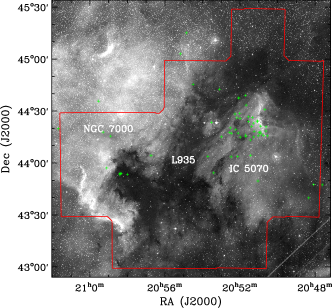
Figure 1.— The location of observation coverage, superimposed on the second Palomar Observatory Sky Survey (POSS II) red image. Green crosses mark the T-Tauri type stars identified by Herbig (1958)

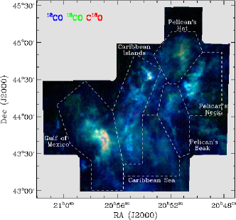
Figure 2.— A composite color image of the NAN complex made from the integrated intensity map, with ¹²CO in blue, ¹³CO in green, and C¹⁸O in red, respectively. The spectra are integrated over $-20\sim 20$ km s^-1 for ¹²CO and ¹³CO, and $-10\sim 10$ km s^-1 for C¹⁸O. We also overlay outlines of the six regions with their names on the plot.

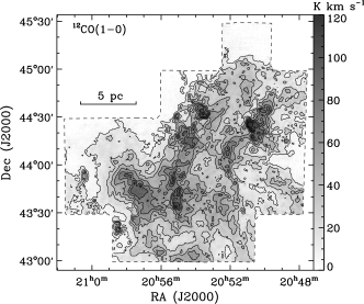
Figure 3.— Integrated intensity contours and gray-scale map of ¹²CO. The spectra are integrated over $-20\sim 20$ km s^-1. The contours are from 10 K km s^-1($\sim 9\sigma$) at intervals of 15 K km s^-1, and the gray-scale colors correspond to a linear stretch of integrated intensity.

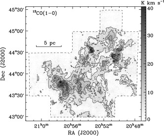
Figure 4.— Integrated intensity contours and gray-scale map of ¹³CO. The spectra are integrated over $-20\sim 20$ km s^-1. The contours are from 4 K km s^-1($\sim 5\sigma$) at intervals of 6 K km s^-1, and the gray-scale colors correspond to a linear stretch of integrated intensity.

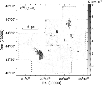
Figure 5.— Integrated intensity contours and gray-scale map of C¹⁸O. The spectra are integrated over $-10\sim 10$ km s^-1. The contours are from 2 K km s^-1($\sim 5\sigma$) at intervals of 1.2 K km s^-1, and the gray-scale colors correspond to a linear stretch of integrated intensity.

The channel map in Figure 6 illustrates the velocity structure of the molecules in the NAN complex. Three ¹³CO filaments are clearly presented in the velocity ranges of $-$7 to $-$4, $-$3 to $-$2, and $-$1 to 0 km s^-1. The latter two filaments connect the Gulf of Mexico and the Pelican’s Hat regions. The emissions in the Gulf of Mexico indicate an arc feature from 0 to 2 km s^-1. Along with the Caribbean Sea, they show complicated structures in the following positive velocity panels. There is another filamentary structure near the Pelican’s Beak, in the velocity range 3 to 4 km s^-1.

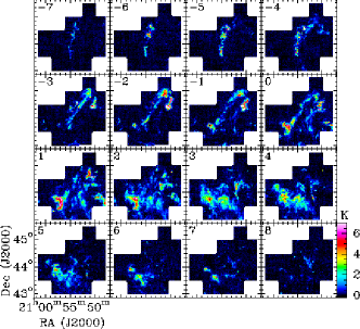
Figure 6.— Channel map of ¹³CO in the NAN complex. The central velocity of each channel, in km s^-1, is marked on the top left corner of each map.

The velocity-coded image shown in Figure 7 indicates the velocity distribution of the emission peak of ¹³CO. Near the center of the whole complex, there are several velocity components with high peak separation, and three filamentary structures showing with different color overlapping each other. The velocity components of the Pelican region in the northwest are relatively simple, while the peak velocities in the southeast show a component around 0 km s^-1, which outlines the Gulf of Mexico region, and another separated extended components at 3-4 km s^-1. Such velocity structure could also be seen on the position-velocity map in Figure 8 along the axis through the full length of the complex in Figure 7. In the center region of the whole complex, the molecular emission near $-$1 km s^-1 is lacking and forms a cavity structure. Bally & Scoville (1980) pointed out that the molecular gas in the northwest part of the NAN complex belongs to an expanding shell surrounding the ionized gas produced by the W80 H II region.

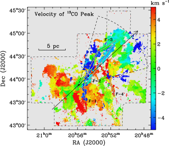
Figure 7.— Velocity-coded ¹³CO map. The color image shows the velocity distribution of the emission peak of ¹³CO. The black long arrow indicates the axis of the position-velocity map in Figure 8. The black dot on the axis indicate the position of the ionizing star. A azimuthally averaged, around the ionizing star within the sector region, position-velocity map is given in Figure 9. The positions of four filamentary structures are shown with white lines.

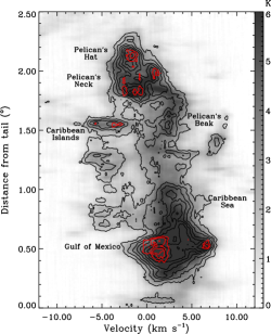
Figure 8.— Position-velocity map along the axis shown in Figure 7. The spectrum on each position is averaged along a 1° width line perpendicular to the axis. The gray-scale background indicates ¹²CO, black contours indicate ¹³CO, and red contours indicate C¹⁸O. The lowest contour is 10$\sigma$ and the contour interval is 10$\sigma$ (0.28 K) for ¹³CO and 5$\sigma$ (0.1 K) for C¹⁸O. Projected positions of six regions are marked.

In Figure 9, we illustrate the kinematic of molecular shell near the Pelican region in detail. We could derive a expansion velocity of $\sim$5 km s^-1. The Pelican’s Hat at the far end is $\sim$14 pc away from the center of the H II region. The cloud near the ionizing star at $\sim$0 km s^-1 connects to the Gulf of Mexico region. Its velocity is close to the rest velocity of the whole complex, which is probably because the molecular gas in these region has not been penetrated by the shock of H II region (Bally & Scoville, 1980). In Figure 8, we could further find there is a velocity gradient of $\sim$0.2 km s^-1 pc^-1 within the complex along the axis of the position-velocity map.

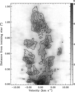
Figure 9.— Azimuthally average position-velocity map around the ionizing star within the sector region shown in Figure 7. The gray-scale background indicates ¹²CO, and black contours indicate ¹³CO. The lowest contour is 5$\sigma$ (0.4 K) and the contour interval is 5$\sigma$.

Our mapping region contains total areas of 403 pc² with ¹²CO detection, 225 pc² with ¹³CO detection, and 18 pc² with C¹⁸O detection over 3$\sigma$ at the distance of 600 pc. Under the assumption of local thermodynamic equilibrium (LTE), we derive the excitation temperature from the radiation temperature of ¹²CO. The distribution of excitation temperature shown in Figure 10 indicates gases of two different temperatures within the NAN complex: localized warm gas ($>$20 K) in the Caribbean Islands, Pelican’s Neck and Beak, and in some small clouds to the southeast; and extended cold gas ($\sim$10 K) distributed throughout the whole of the dark nebula. The warm gas clearly matches the edge of the whole cloud, suggesting the warm clouds are heated by the background H II regions.

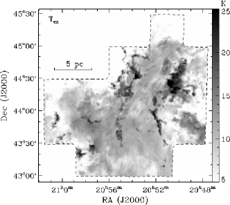
Figure 10.— A gray-scale map of excitation temperature in the NAN complex. The excitation temperature is derived from the radiation temperature of ¹²CO within the velocity range of $-20\sim 20$ km s^-1.

We further calculate the column density and LTE mass with the ¹³CO data following the process given by Nagahama, Mizuno, Ogawa et al. (1998) and adopting a ¹³CO abundance of $N({\rm H_{2}})/N({\rm{}^{13}CO})=7\times 10^{5}$. We obtain a total mass of $2.0\times 10^{4}~{}M_{\odot}$ in the NAN complex. Using the abundance of $N({\rm H_{2}})/N({\rm C^{18}O})=7\times 10^{6}$ (Castets & Langer, 1995), a LTE mass based on C¹⁸O data can also be derived as $6.1\times 10^{3}~{}M_{\odot}$. If we simply use the CO-to-H₂ mass conversion factor $X$ of $1.8\times 10^{20}~{}{\rm cm^{-2}(K~{}km~{}s^{-1})^{-1}}$ given in the CO survey of Dame, Hartmann, & Thaddeus (2001), a mass of $5.4\times 10^{4}~{}M_{\odot}$ can be derived for the complex. The mass of inner denser gas traced by ¹³CO accounts for 36% of the mass in a larger area traced by ¹²CO, while the mass in a few small dense cloud traced by C¹⁸O accounts for 11% of the total mass.

In our calculation, we obtained a mean H₂ column density of $5.8\times 10^{21}$ cm^-2 based on ¹²CO emission by averaging all pixels with line detection. Similar method produces a mean column density of 3.4, and 11.9$\times 10^{21}$ cm^-2 traced by ¹³CO and C¹⁸O, respectively. We show the surface density map for the three molecular species in Figure 11. All three tracers show a maximum surface density over 500 $M_{\sun}$ pc^-2 in the Pelican’s Neck region, while the Gulf of Mexico region is optically thick with high surface density only in the C¹⁸O map. The $3\sigma$ noise at $T_{\rm ex}=10$ K within velocity width of 40 km s^-1 correspond to 14, 19, and 146 $M_{\odot}$ pc^-2 in ¹²CO, ¹³CO, and C¹⁸O map, respectively. Therefore the mass hidden under our detection limit of ¹³CO is lower than $5.4\times 10^{2}~{}M_{\odot}$, which indicates that the discrepancy in the obtained mass between ¹²CO and ¹³CO is mainly the result of the different emission area tracing by them. The hidden mass for C¹⁸O is $1.4\times 10^{3}~{}M_{\odot}$ at most, significantly lower than the total mass traced by ¹³CO. This means that we have detected over 80% of mass in our C¹⁸O observation area.

Bally & Scoville (1980) observed a similar field in the NAN complex and estimated the LTE mass as $(3-6)\times 10^{4}~{}M_{\odot}$ for a distance of 1 kpc and ¹³CO abundance of $N({\rm H_{2}})/N({\rm{}^{13}CO})=1\times 10^{6}$. For the same parameters as we used, it would correspond to (1-2)$\times 10^{4}~{}M_{\odot}$. Cambrésy, Beichman, Jarrett et al. (2002) obtained a mass of $4.5\times 10^{4}~{}M_{\odot}$ for a distance of 580 pc in their near-infrared extinction study covering an area of 6.25 deg² in the NAN complex. These discrepancy of mass might be due to the dust-to-gas ratio or the $X$ factor.

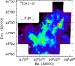
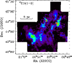
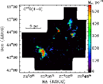
Figure 11.— The surface density of H₂ traced by ¹²CO, ¹³CO, and C¹⁸O with the same dynamical range. The abundance $N({\rm H_{2}})/N({\rm{}^{13}CO})=7\times 10^{5}$ (Nagahama, Mizuno, Ogawa et al., 1998) and $N({\rm H_{2}})/N({\rm C^{18}O})=7\times 10^{6}$ (Castets & Langer, 1995) are adopted in the surface density calculation.

3.2. Features in Individual Regions

Several discernible regions and filamentary structures can be identified in our observations. The spectra observed toward the regions are shown in Figure 12. The variety of line profile and intensity ratios indicates distinct kinematic and chemistry environments. Their properties probed by different tracers are summarized in Table 2 and details for each region are listed below.

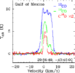
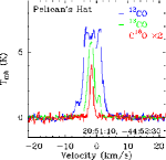
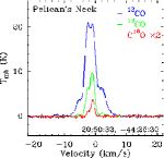
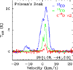
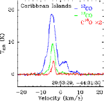
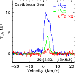
Figure 12.— Typical spectra in the selected regions with names in the upper left corner. These spectra are averaged within a 2′$\times$2′ box centered at the positions (RA, Dec) marked at the lower right corner.

Table 2Properties of regions

			12CO				13CO					C18O
Region	$T_{\rm ex}$		area	$N_{\rm H_{2}}$	$M$		area	$N_{\rm H_{2}}$	$M$	$\Delta v$		area	$N_{\rm H_{2}}$	$M$		$S({\rm C^{18}O})\over S({\rm{}^{13}CO})$
	(K)		(pc2)	($10^{22}{\rm cm}^{-2}$)	($10^{3}M_{\odot}$)		(pc2)	($10^{22}{\rm cm}^{-2}$)	($10^{3}M_{\odot}$)	(km s-1)		(pc2)	($10^{22}{\rm cm}^{-2}$)	($10^{2}M_{\odot}$)
Gulf of Mexico	14.2		18.2	1.2	11.8		5.7	1.3	5.4	5.93		2.0	2.5	32.0		0.13
Pelican’s Hat	12.2		16.4	0.7	4.1		4.6	0.6	1.7	4.37		1.3	1.3	8.4		0.14
Pelican’s Neck	22.8		4.4	1.6	6.0		3.4	1.6	3.1	2.99		0.6	2.4	9.9		0.07
Pelican’s Beak	15.9		7.5	1.1	4.8		2.2	0.8	1.3	2.24		0.3	1.1	1.3		0.08
Caribbean Islands	18.7		19.2	1.3	12.3		2.2	1.3	5.0	2.98		0.3	3.6	8.5		0.11
Caribbean Sea	12.1		41.6	0.7	8.1		10.2	0.4	2.5	3.86		-	-	-		-

Note. — The properties of the regions in the NAN complex, including excitation temperature, area within the half maximum contour line, mean column density of H₂, and mass of ¹²CO, ¹³CO, and C¹⁸O, line width of averaged spectra for ¹³CO, and integrated intensity ratio of C¹⁸O to ¹³CO. The column density and mass for ¹²CO are derived with a constant CO-to-H₂ mass conversion factor, and those for ¹³CO, and C¹⁸O are derived under the LTE assumption. The C¹⁸O properties in Caribbean Sea is missing because of the low C¹⁸O detection rate in this region.

The “Gulf of Mexico” (GoM) is the largest and the most massive region with all three line detections in the southeast of the NAN complex. Two major clumps can be found in this region: one in the north (GoM N) with weak C¹⁸O emission, and one in the south (GoM S), with strong C¹⁸O emission indicating a pair of parallel arcs, which closely matches the morphology of the filamentary dark cloud in Spitzer mid-infrared image (Guieu, Rebull, Stauffer et al., 2009; Rebull, Guieu, Stauffer et al., 2011). The ¹²CO spectra are flat-topped, indicating high opacity at these locations. Under the LTE assumption, we find a low excitation temperature ($\sim$14 K), large line width, and high column density in this region. The intensity ratio in Figure 13, which also indicates the relative abundance of C¹⁸O to ¹³CO, shows a higher ratio in the GoM S. Rebull, Guieu, Stauffer et al. (2011) reported a young stellar objects (YSOs) cluster is associated with the GoM region. A high concentration of T-Tauri type stars (Herbig, 1958) and an association of H₂O maser (Toujima, Nagayama, Omodaka et al., 2011) are found in the GoM N. No IRAS point sources are associated with either clump. These evidence suggest active star formation in the GoM region, and the GoM N region is relatively more evolved than GoM S.

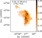
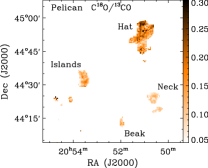
Figure 13.— Integrated intensity ratio of C¹⁸O to ¹³CO. The two panels show the same region as that in Figure 5. Names of the regions are marked on the map.

The “Pelican”s Hat” locates to the north of Pelican’s head, and is similar to but smaller than the GoM S. The excitation temperature in this region is low ($\sim$12 K), and the relative abundance of C¹⁸O to ¹³CO is higher than those in other regions in Pelican nebula. The line emission resembles the morphology of mid-infrared extinction in Spitzer image (Guieu, Rebull, Stauffer et al., 2009; Rebull, Guieu, Stauffer et al., 2011).

The “Pelican”s Neck” region to the west of the NAN complex shows the most intense ¹²CO emission in our survey. It presents a high excitation temperature of $\sim$23 K, narrow line width, and weak C¹⁸O emission. The molecular emission shows a bright feature oriented in the north-south direction, with a sharp cut-off towards the east. Several IRAS sources are associated with the peaks on the ¹³CO map. A position-velocity slice along the east edge of the Pelican’s Neck (as in Figure 14) reveals a weak component at $\sim$3 km s^-1 that is separate from the molecular clump and forms a cavity near IRAS 20489+4410 and IRAS 20490+4413 in the velocity dimension. Such a structure could be the result of an embedded H II region.

The molecular emission in Pelican’s Neck matches the morphology of the brightest surface brightness region in Spitzer mid-infrared image, and it is at the west edge of the Pelican Cluster, an active star forming cluster of YSOs identified by Rebull, Guieu, Stauffer et al. (2011). A clustering of T-Tauri type stars (Herbig, 1958) was found around the molecular clump. These all indicate that the Pelican’s Neck is a warm region with active star formation.

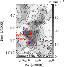
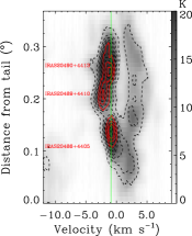
Figure 14.— Left: the ¹³CO integrated intensity map of Pelican’s Neck. Red stars indicate the position of IRAS point sources. The names of three massive sources are indicated. The blue arrow indicates the axis of the position-velocity map. Right: position-velocity map along the axis shown in the left panel. The gray-scale background indicates ¹²CO, dashed contours indicate ¹³CO, and red solid contours indicate C¹⁸O. The lowest contour is 10$\sigma$ and the contour interval is 15$\sigma$ for ¹³CO and 10$\sigma$ for C¹⁸O. The vertical green line indicates the rest velocity averaged over the whole region. Projected positions of three IRAS sources are marked.

The “Pelican”s Beak” region is a small elongated region to the southeast of Pelican’s Neck. The excitation temperature is intermediate ($\sim$15 K) with weak C¹⁸O emission. The molecules protrude along a filament to the south at the velocity of 3 km s^-1. Its properties may suggest an intermediate stage between the cold dense regions (e.g. GoM, Pelican’s Hat) and the warm active regions (e.g. Pelican’s Neck, Caribbean Islands).

The “Caribbean Islands” are several bright clumps extending from the west of GoM and to the east of Pelican’s head. The southern half of Caribbean Islands is spatially coincident with the Caribbean Sea. The channel map indicates these “Islands” are part of a filamentary structure (see 3.3). They associate with several highly localized nebulous bright blobs in Spitzers mid-infrared image (Rebull, Guieu, Stauffer et al., 2011). These clumps show a high excitation temperature, narrow line width, and low relative abundance of C¹⁸O. These properties indicate a similar situation to that in Pelican’s Neck. Together with Pelican’s Neck, the north part of Caribbean Islands forms a cavity structure at the position of the Pelican Cluster which can be seen on the ¹³CO integrated intensity map.

The molecular cloud in the northernmost part of this region is associated with an H II regions, G085.051$-$0.182 at $-0.2$ km s^-1, identified by Lockman, Pisano, & Howard (1996). Figure 15 shows that the H II region is not associated with any dense molecular clumps at its rest velocity. Dense and heated gas with temperature $\sim$27 K appears within the velocity from $-$6 to $-3$ km s^-1 near the position of the H II region, while diffuse clumps are shown in the panels with positive velocities. The position-velocity map shows an incomplete asymmetric molecular shell around the H II region. It is notable that the densest part of the heated clumps tracing by C¹⁸O presents a slightly higher velocity, which is closer to the rest velocity of the H II region than those tracing by ¹²CO and ¹³CO. These indicate that the H II region undergoes an asymmetric expansion within the parent molecular cloud.

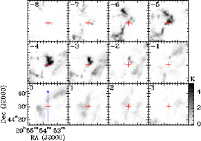
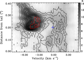
Figure 15.— Top: channel map of ¹³CO near H II region in the Caribbean Islands region. The cross in each panel marks the position of the H II region, G085.051$-$0.182, reported by Lockman, Pisano, & Howard (1996). The central velocity of each channel, in km s^-1, is marked on the top left corner of each map. The blue arrow is the axis of the position-velocity map. Bottom: position-velocity map along the axis shown in the top panel. The gray-scale background indicates ¹²CO, dashed contours indicate ¹³CO, and red solid contours indicate C¹⁸O. The lowest contour is 5$\sigma$ for ¹³CO and 10$\sigma$ for C¹⁸O, with the contour interval of 5$\sigma$. The cross indicates the rest velocity and the position of the H II region.

The “Caribbean Sea” is a diffuse extended cloud to the west of GoM at the velocity of 3 km s^-1 with low excitation temperature and optical depth. ¹²CO are detected in a large area, and weak C¹⁸O emission can only be detected at a few positions. This region shows the lowest column density among all the regions but its total mass is relatively high.

3.3. Filamentary Structures

In our observations with velocity dimensions, we resolve three separate filamentary structures (designated as F-1, F-2, F-3 in ascending velocity order) nearly parallel to each other along the dark lane in the NAN complex. Another filament (F-4) is also resolved near Pelican’s Beak region. Figure 7 shows the positions of the filaments with different color representing their different velocity. Figure 16 and 17 shows the morphology and velocity structure of these filaments. We found elongated molecular clumps along these filaments. F-1, which contains the bright clumps in Caribbean Islands, presents a complex twisted spatial and velocity structure, with a ring-like structure near $\rm 20^{h}54^{m}.5,+44^{\circ}19^{\prime}$. F-2 and F-3 are discontinuous, and together with the Pelican’s Hat region, they form a hub-filament structure (Myers, 2009). The northwest and the southeast section of F-2 show opposite velocity gradient directions. The northwest section of F-3 bends to the east with higher velocity and surrounds the Pelican Cluster. Both F-2 and F-4 show clear velocity gradient along their axes in the position-velocity map.

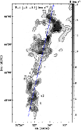
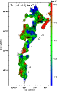
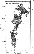
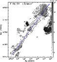
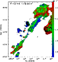
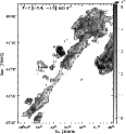
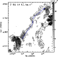
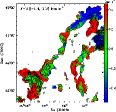
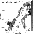
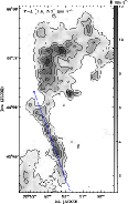
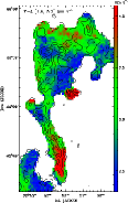
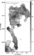
Figure 16.— ¹³CO moment maps of the filaments showing the integrated intensity (left), rest velocity (middle), and line width (right). On each panel, the zeroth moment contour lines are overlaid from 7$\sigma$ with 10$\sigma$ intervals. The name and the velocity range of each filament is marked in the top left corner in each panel.

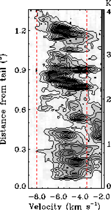
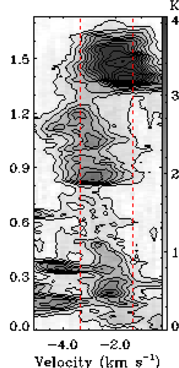
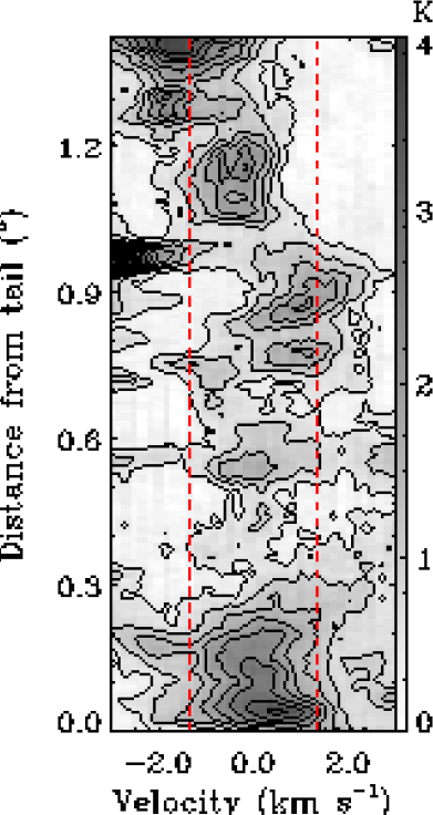
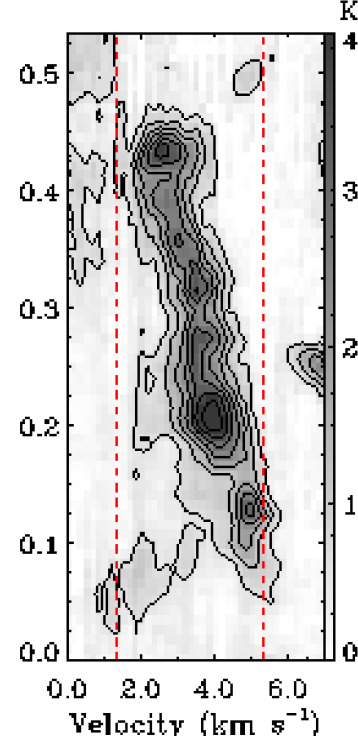
Figure 17.— ¹³CO position-velocity map of the four filamentary structures along the axes shown in the integrated intensity maps of Figure 16. The lowest contour is 5$\sigma$ and the contour interval is 5$\sigma$ for each panel. Red dashed lines indicate the velocity range of each filaments.

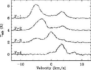
Figure 18.— Position averaged ¹³CO spectra of the filaments. Spectra are moved upwards for clarity. The name of each filament is marked on the left of each spectrum.

We show the averaged spectra in Figure 18 and some physical properties of the filaments are listed in Table 3. A typical ¹³CO line width of 3.3 km s^-1 is shown. These filamentary structures show similar optical depths, while F-1 and F-4 have a higher excitation temperature. We could estimate the mass per unit length by dividing the mass of filaments by their spatial dimension. F-1 shows a higher mass per unit length than that in the other filaments. The twisted structure in F-1 may cause an overestimation of this measurement. A maximum, critical linear mass density needed to stabilize a cylinder structure can be calculated with $(M/l)_{\rm max}=84(\Delta v)^{2}M_{\odot}{\rm pc}^{-1}$ in the turbulent support case, where $\Delta v$ is the line width in unit of km s^-1 (Jackson, Finn, Chambers et al., 2010). This means our filaments are gravitationally stable on the assumption of the ¹³CO abundance we adopted.

Table 3Properties of filaments

Filament	$T_{\rm ex}$	$\Delta v$(13CO)	$\tau$(13CO)	$M$	$M/l$
	(K)	(km s-1)		($M_{\odot}$)	($M_{\odot}$ pc-1)
F-1	16	3.20	0.33	1401	107
F-2	12	3.77	0.34	416	30
F-3	12	3.52	0.36	487	32
F-4	17	2.75	0.26	196	38

Note. — The properties of the filaments in the NAN complex, including excitation temperature, line width of averaged spectra, optical depth of ¹³CO, mass, and mass per unit length. These typical values are the results averaged within the 10$\sigma$ contour line of each filament.

3.4. Clump Identification

We use the FINDCLUMPS tool in the CUPID package (a library of Starlink package) to identify molecular clumps in the obtained ¹³CO FITS cube. The ClumpFind algorithm is applied in the process of identification. The algorithm first contours the data and searches for peaks to locate the clumps, and then follows them down to lower intensities. We set the parameters TLOW=5$\times$RMS and DELTAT=3$\times$RMS, where TLOW determines the lowest level to contour a clump, and DELTAT represents the gap between contour levels which determines the lowest level at which to resolve merged clumps (Williams, de Geus, & Blitz, 1994). The parameters of each clump, such as the position, velocity, size in RA and Dec directions, and one-dimensional velocity dispersion, are directly obtained in this process. The clump size has removed the effect of beam width, and velocity dispersion is also de-convolved from the velocity resolution. The morphology of the clumps are checked by eye within the three-dimension RA-Dec-velocity space to pick out clumps with meaningful structures. We then mark every clump on their velocity channel in the ¹³CO cube to confirm the morphology and emission intensity of the molecular gas within the clumps. In addition, clumps with pixels that touch the edge of the data cube are removed. 22 clumps are removed in these checking steps. Eventually, a total of 611 clumps are identified, and the position, velocity, and size of the clumps as illustrated in Figure 19 are consistent with the spatial and velocity distribution of the molecular gas.

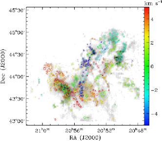
Figure 19.— Clumps identified in ¹³CO data cube. The circles indicate the clump positions on the integrated intensity map of ¹³CO. The colors of the circles represent the velocities the clumps, while the circles are scaled according to the sizes of clumps.

We extract the excitation temperature for each clump from their ¹²CO datacube under LTE assumption and can then derive the LTE mass. The parameters of the clumps are listed in Table 4. The clump size are derived from the geometric mean of the clump size in two directions. Figure 20 shows the distributions of clump size, excitation temperature, and volume density, which yield typical properties of $\sim$0.3 pc, 13 K, and 8$\times 10^{3}$ cm^-3, respectively. The left panel in Figure 21 shows the distribution of three-dimensional velocity dispersion estimated as $\sigma_{v\rm 3D}=\sqrt{3}\sigma_{v\rm 1D}$. The thermal portion in the velocity dispersion is $\sigma_{\rm Thermal}=\sqrt{kT_{\rm kin}/m}$, where $k$ is the Boltzmann constant, $m$ is the mean molecular mass, and $T_{\rm kin}$ is the kinetic temperature equal to the excitation temperature, while the non-thermal portion is $\sigma_{\rm Non-thermal}=\sqrt{\sigma_{v\rm 1D}^{2}-\sigma_{\rm Thermal}^{2}}$. The distribution of the thermal and non-thermal velocity dispersion are shown in Figure 21. There are 568 (93%) clumps with $\sigma_{\rm Non-thermal}$ larger than $\sigma_{\rm Thermal}$. The mean ratio of $\sigma_{\rm Non-thermal}$ and $\sigma_{\rm Thermal}$ is 1.57. This suggests that non-thermal broadening mechanisms (e.g., rotation, turbulence, etc) play a dominant role in the clumps.

Table 4Properties of clumps

Clump	R.A.	Dec.	Velocity	$\Delta{\rm R.A.}$	$\Delta{\rm Dec.}$	$R$	$\delta_{v\rm 1D}$	$T_{\rm peak}$	$T_{\rm ex}$	$\Sigma$	$n_{\rm H_{2}}$	$M_{\rm LTE}$	$\alpha_{\rm Vir}$
	(J2000)	(J2000)	(km s-1)	(″)	(″)	(pc)	(km s-1)	(K)	(K)	($M_{\sun}\rm pc^{-2}$)	$10^{3}\rm cm^{-3}$	($M_{\odot}$)
1	20 48 01.2	+43 42 59.4	+0.01	115.9	120.7	0.17	0.35	4.40	16.67	23.9	11.2	15.6	1.52
2	20 48 01.6	+43 34 43.8	+1.13	139.2	178.4	0.23	0.35	4.57	17.73	31.9	10.1	33.2	0.98
3	20 48 15.2	+43 40 59.4	+1.50	128.9	160.3	0.21	0.24	3.62	15.32	17.0	5.2	13.1	1.07
4	20 48 20.6	+43 31 04.7	+0.99	56.5	94.2	0.10	0.28	3.27	14.66	6.9	5.6	1.8	5.00
5	20 48 37.6	+43 48 11.8	+1.01	194.6	319.4	0.36	0.56	3.73	18.72	40.1	5.7	74.4	1.74
6	20 48 41.2	+43 39 38.6	+1.67	52.0	31.2	0.06	0.21	7.21	14.41	9.8	29.7	1.6	1.80
7	20 48 42.3	+44 21 38.6	$-$4.26	47.5	65.4	0.08	0.36	5.19	17.79	15.3	26.4	3.9	3.09
8	20 48 44.2	+43 40 15.1	+2.25	32.2	79.2	0.07	0.19	6.69	13.16	7.2	10.6	1.2	2.58
9	20 48 44.8	+43 52 52.4	+1.47	169.5	193.1	0.26	0.27	3.61	16.00	17.9	3.0	14.8	1.46
10	20 48 46.3	+44 15 17.7	+1.95	45.3	80.5	0.09	0.40	6.49	24.47	38.2	53.3	9.9	1.63

Note. — The properties of the clumps in the NAN complex. Columns are clump number, clump position (R.A. and Dec.), rest velocity, clump size in R.A. and Dec. direction, clump radius, one-dimensional velocity dispersion, temperature of emission peak, excitation temperature, surface density, volume density, LTE mass, and virial parameter. The entire table is published in its entirety in the electronic edition. A portion is shown here for guidance regarding its form and content.

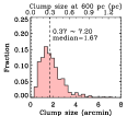
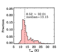
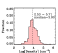
Figure 20.— Distribution of clump size (left), excitation temperature (middle), and volume density (right). The size is the geometric mean of the size in the R.A. and Dec. direction, and density is derive under the spherical assumption. The range and typical value of each property are marked on each plot.

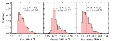
Figure 21.— Histogram of three-dimensional velocity dispersion (left), and the thermal (middle) and non-thermal (right) one dimensional velocity dispersions. The range and typical value of each velocity dispersion are marked on each panel.

4. Discussion

4.1. Comparison with Other Star Formation Regions

In a typical low-mass star-forming region, the Taurus region, Goldsmith, Heyer, Narayanan et al. (2008) gives a LTE column density of $\leq 10^{22}$ cm^-2 for the most dense region based on the data from the Five College Radio Astronomy Observatory (FCRAO) survey (Narayanan, Heyer, Brunt et al., 2008). This column density is lower than the averaged column density we derived in several dense regions of the NAN complex. Qian, Li, & Goldsmith (2012) searched for clumps in the Taurus survey data and derived a typical mean H₂ density of $\sim$2000 cm^-3, lower than the clump density in NAN complex of 8000 cm^-3. In addition, we found a number of clumps with densities over 10⁴ cm^-3, which is hardly seen in the Taurus region. The ¹³CO line width (0.4-2.2 km s^-1) in NAN complex is also slightly higher than that in Taurus (0.5-1.7 km s^-1). These may indicate potential massive stars are forming in some of the dense clumps in the NAN complex.

In an active high-mass star-forming region, such as the Orion Nebula, a survey of the Orion A region by Nagahama, Mizuno, Ogawa et al. (1998) yielded an averaged column density similar to our results. Their survey found regions with excitation temperature $\geq$ 20 K in most areas, and an even higher temperature of $\geq$ 60 K in the Orion KL region. Meanwhile, the high temperature regions in the NAN complex are limited to those around the Pelican Cluster. In fact, the statistical properties of the clumps we identified in the NAN complex are similar to those of the Planck cold dense core (Planck Collaboration, Ade, Aghanim et al., 2011) of the Orion complex as studied by Liu, Wu, & Zhang (2012). These results suggest most of the clumps, especially the cold ones, in the NAN complex are in an early evolutionary stage of star formation dominated by a non-thermal environment.

4.2. Gravitational Stability of the Clumps

The gravitational stability of clump determines whether the molecular clump could further collapse and form a star cluster. We firstly calculate the escape velocity ($v_{\rm escape}=\sqrt{2GM_{\rm LTE}/R}$) for each clump and compare with its three-dimensional velocity dispersion. The escape velocities range from 0.21 to 2.84 km s^-1 with a typical value of 0.64 km s^-1. About 493 (72%) clumps have velocity dispersion smaller than escape velocity, and only 8 (1%) clumps have velocity dispersion larger than twice the escape velocity. We note that the clumps with high $\sigma_{v\rm 3D}$ to $v_{\rm escape}$ ratios are faint with low emission peaks.

By simply assuming the clumps have a density profile of $\rho(r)=r^{-k}$ with power-law index $k=1$, we could further derive the virial mass using the standard equation (e.g. Solomon, Rivolo, Barrett et al. 1987; Evans 1999): $M_{\rm Vir}=1164R\sigma_{v\rm 1D}^{2}[M_{\odot}]$, where the clump size $R$ is in pc, and three-dimensional velocity dispersion $\sigma_{v\rm 1D}$ is in km s^-1. A steeper power-law index of $k$ would result in a lower estimation of virial mass. The virial parameter, defined as the ratio of virial mass to LTE mass: $\alpha_{\rm Vir}=M_{\rm Vir}/M_{\rm LTE}$, describes the competition of internal supporting energy against the gravitational energy. We find a typical virial parameter of 2.5 in our clump sample. The virial masses are comparable to the LTE masses. There are 588 (96%) clumps with virial mass larger than LTE mass, and 221 (36%) clumps with virial parameter larger than 3. The clumps with high virial parameter ($\alpha_{\rm Vir}>10$) are all faint ones with emission peak lower than 3.3 K. The clumps with $\alpha_{\rm Vir}<1$ are virialized and could be collapsing, while the clumps with higher $\alpha_{\rm Vir}$ could be in a stable or expanding state unless they are external pressure confined. Alternatively, it is possible that the faint clumps may be transient entities (Ballesteros-Paredes, 2006).

Figure 22 shows the spacial distribution of clumps with virial parameter coded. It is notable that the clumps close to virial equilibrium associate with dense gas mainly around the Pelican region. The clumps in the Gulf of Mexico region present slightly higher virial parameters than those in the other dense regions, and most of the clumps with weak molecular emissions especially those in the Caribbean Sea region are far from equilibrium state. We compare $M_{\rm Vir}$ and $M_{\rm LTE}$ in the left panel of Figure 23. The massive clumps tend to have a lower virial parameter. The mass relationship can be fitted with a power-law of $M_{\rm Vir}/(M_{\odot})=(4.26\pm 0.16)[M_{\rm LTE}/(M_{\odot})]^{(0.75\pm 0.02)}$. The power index we obtained is slightly higher than the value in Orion B (0.67) reported by Ikeda & Kitamura (2009) and Planck cold clumps (0.61) reported by Liu, Wu, & Zhang (2012), moreover, significantly higher than the index of pressure-confined clumps ($\alpha_{\rm Vir}\propto M_{\rm LTE}^{-2/3}$) as given by Bertoldi & McKee (1992). Although our molecular observations reveal several clumps in the NAN complex could be exposed to strong external pressure from ionising radiation and winds of massive stars, the comparability and the high power index of virial and LTE mass suggest that most molecular clumps in the NAN complex are gravitationally bound rather than pressure confined.

We could also derived the Jeans mass with $M_{\rm Jeans}=17.3{T_{\rm kin}}^{1.5}n^{-0.5}M_{\odot}$ (Gibson, Plume, Bergin et al., 2009) and plot their relationship with LTE mass in the right panel of Figure 23. Such relationship could be described with a power-law of $M_{\rm Jeans}/(M_{\odot})=(7.82\pm 0.27)[M_{\rm LTE}/(M_{\odot})]^{(0.12\pm 0.01)}$. The flat power index indicates that the LTE masses of most massive clumps are substantially larger than their Jeans mass, suggesting that these clumps will further fragment and may not form individual proto-stars but proto-clusters.

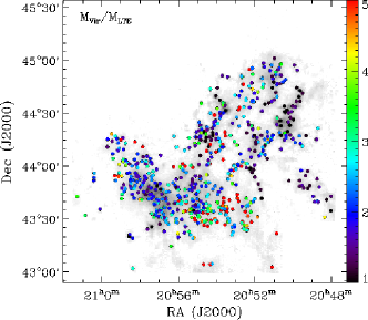
Figure 22.— Distribution of clumps with virial parameter coded. The dots represent the clumps overlaid on the integrated intensity map of ¹³CO. The colors of the dots indicate the virial parameter of the clumps.

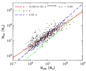
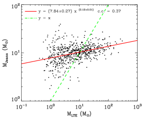
Figure 23.— Top: Virial mass-LTE mass relation of the clumps. Bottom: Jeans mass-LTE mass relation of the clumps. The dot-dashed green line indicates a mass ratio of 1. The solid red line shows a power-law fit to the relationship. The dashed blue line in the left panel indicates the median mass ratio.

4.3. Larson Relationship and Mass Function of Clumps

Larson (1981) presents a correlation between the velocity dispersion and the region size (range from 0.1 to 100 pc), known as the Larson relationship. The Larson relationship was suggested to exist by several work (Leung, Kutner, & Mead, 1982; Myers, Linke, & Benson, 1983), but some recent molecular surveys suggest weak or no correlation between line width and size of molecular clouds (Onishi, Mizuno, Kawamura et al., 2002; Liu, Wu, & Zhang, 2012). Figure 24 shows the relationship between size and three dimensional velocity dispersion for our clumps. A fitting to the data gives a correlation of $\sigma_{v\rm 3D}/({\rm km~{}s^{-1}})=(1.00\pm 0.03)\times[{\rm Size}/({\rm pc})]^{(0.43\pm 0.02)}$, with a correlation coefficient of 0.63. The power index is slightly larger than 0.39 given by Larson (1981). The correlation is not strong, which might be the result of small dynamic range, and of the scattering of velocity dispersion and clump size (0.06-1.26 pc) we found. The dynamic range is limited by the sensitivity of observations. A uniform survey with sufficient high sensitivity will improve the completeness of less intense clumps with low column density and small size. On the other hand, Liu, Wu, & Zhang (2012) pointed out that turbulence plays a dominant role in shaping the clump structures and density distribution at a large scale, while the small-scale clumps are easily affected by the fluctuations of density and temperature. This will cause a large scattering of line width broadening induced by other factor other than turbulence at small scales. Such scattering of the velocity dispersion may result in a weak or even absent relationship.

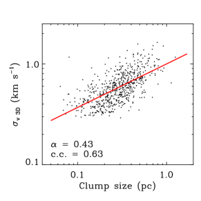
Figure 24.— Larson relationship for the clumps. The red line indicates a linear fitting to the clump size and velocity dispersion relation.

We then study the clump mass function (CMF) in Figure 25 based on the clump mass sample we derived. A power-law distribution of d$N$/d log$M\propto M^{-\gamma}$ is fitted with our data. Our power index (0.95) is lower than the stellar initial mass function (IMF) of 1.35 give by Salpeter (1955). Several (sub)millimeter continuum studies (Testi & Sargent, 1998; Johnstone & Bally, 2006; Reid & Wilson, 2006) and molecular observations (Ikeda & Kitamura, 2009) obtained CMFs which are consistent with the Salpter IMF, while Kramer, Stutzki, Rohrig et al. (1998) reported a flatter power index of 0.6-0.8 in their CO isotopes study of seven molecular clouds. The similarity between CMF and IMF power indices could simply be explained by a constant star formation efficiency unrelated to the mass and self-similar cloud structure, based on a scenario of one-to-one transformation from cores to stars (Lada, Muench, Rathborne et al., 2008). However, such scenario is oversimplified, and ignores the fragmentation in cores whose masses exceed the Jeans mass. Fragmentation in prestellar cores has been observed and discussed by several work (Goodwin, Kroupa, Goodman et al., 2007; Chen & Arce, 2010; Maury, André, Hennebelle et al., 2010). In addition, a simulation by Swift & Williams (2008) suggested that the obtained IMF is similar to the input CMF even when different fragmentation modes are considered.

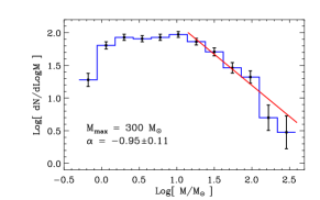
Figure 25.— Clump mass function (CMF) for the clumps. Red line fit the power-law distribution from 15 to 300 M_⊙.

4.4. YSOs in Molecular Cloud

Cambrésy, Beichman, Jarrett et al. (2002) identified nine young stellar clusters in the NAN complex, and Guieu, Rebull, Stauffer et al. (2009) provided a list of more than 1600 YSOs in their four Infrared Array Camera (IRAC) bands study with the Spitzer Space Telescope. Lately, Rebull, Guieu, Stauffer et al. (2011) incorporated their Multiband Imaging Photometer for Spitzer (MIPS) observations with earlier archival data, and identified a list of 1286 YSOs in the NAN complex. We compare the distribution of the YSOs from Rebull, Guieu, Stauffer et al. (2011) with our molecular observations in Figure 26. The Class I and flat sources are concentrated in cold and dense molecular clouds, especially in the Gulf of Mexico and the Pelican’s Hat region, while the Class II sources are spread across the cloud with low molecular opacity, and only a few YSOs are associated with the diffuse Caribbean Sea region. The molecular properties associated with different classes of YSOs are extracted and studied in Figure 27. The histograms indicate that the Class I and flat sources match the distribution of molecular clouds and prefer a cold dense environment with excitation temperature of $\sim$14 K and column density of $\sim$10²² cm^-2.

Three main YSO clusters are identified from the sample of Rebull, Guieu, Stauffer et al. (2011). Two of these with a great fraction of Class I and flat objects are associated with the molecular cloud of the Gulf of Mexico and the Pelican’s Hat region which shows low temperature and high C¹⁸O abundance. The third cluster, the Pelican Cluster, is surrounded by the Pelican’s Neck, the Pelican’s Beak, and the Caribbean Islands. Although the Class II sources constitute a higher fraction in the Pelican Cluster, most of the Class I and flat objects appear on the east and west edges of the cluster. This distribution is consistent with the molecular distribution in which the molecular gas in the central area is dispersed and surrounded by clouds with higher molecular temperature and low C¹⁸O abundance. The YSO proportion in the clusters suggests a younger stage of evolution in the most south-eastern and north-western parts of the NAN complex, and an older stage in the center of the Pelican Cluster. If the complex velocity structures in surrounding regions of the Pelican Cluster are indeed the results of feedbacks from the massive cluster members, the cluster may be triggering the star formation in the molecular cloud across a span of over 5 pc and $\sim$10 km s^-1.

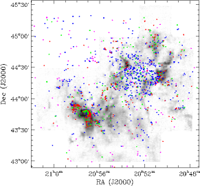
Figure 26.— YSOs in the NAN complex identified by Rebull, Guieu, Stauffer et al. (2011). The gray-scale image is the integrated intensity map of ¹³CO. Red dots are Class I, green are flat, blue are Class II, and purple are Class III.

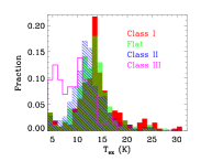
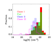
Figure 27.— The molecular properties (left: excitation temperature; right: column density of H₂) associated with YSOs, with the same color code as Figure 26.

We then compare our clump results with the distribution of YSOs, by separating the clumps spatially associated with YSOs from those containing no YSO. The Class III YSOs are not considered, as the Class III catalogue is not complete and their distribution is not associate with molecular cloud. A total of 143 clumps are found to be associated with YSOs. The discrepancies in their physical properties are shown in Figure 28. The clumps associated with YSOs present a higher velocity dispersion, clump size, and excitation temperature, while the discrepancy of the CMF indices is not significant. Further observations with higher signal-to-noise ratio and resolution are needed to extend the limit of mass completeness in CMF comparison.

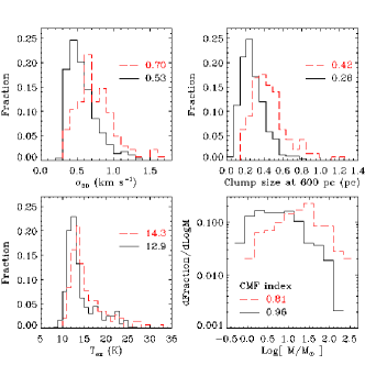
Figure 28.— The histogram of three-dimensional velocity dispersion (upper left), clump size (upper right), excitation temperature (lower left) and CMF (lower right). Red lines represent the clumps associated with YSOs, while black lines represent the clumps without YSOs. The median values and CMF indices are marked on the plot.

5. Summary

We have presented the PMODLH mapping observations for an area of 4.25 deg² toward the North American and Pelican Nebulae molecular cloud complex in ¹²CO, ¹³CO, and C¹⁸O lines. The main results are listed below:

The molecules distribution is along the dark lane in the southeast-northwest direction. ¹²CO emission is bright, extended, while ¹³CO and C¹⁸O emissions are compact. The channel map shows intricate structures within the complex, and filamentary structures are revealed. Position-velocity slice along the full length of the cloud reveals a molecular shell surrounding the W80 H II region. Gases of two different temperatures are seen in the distribution of excitation temperature.

The surface density map shows several dense clouds with surface density over 500 $M_{\sun}$ pc^-2 in the complex. We have derived a total mass of $2.0\times 10^{4}~{}M_{\odot}$ (¹³CO) and $6.1\times 10^{3}~{}M_{\odot}$ (C¹⁸O) under the LTE assumption with uniform molecular abundance, and $5.4\times 10^{4}~{}M_{\odot}$ with the constant CO-to-H₂ factor in the NAN complex. Such a discrepancy in mass may be due to the different extent which the molecules are tracing.

Six regions are discerned in the molecular maps, each with different emission characteristics. Their sizes, column densities, and masses vary with different density tracers. The properties of low temperature, high column density, and high C¹⁸O abundance found in the Gulf of Mexico, and Pelican’s Hat regions indicate a young stage of massive star formation, while the properties of the Pelican’s Neck, Pelican’s Beak, and Caribbean Islands regions represent a hot, dense, and more evolved environment probably affected by the Pelican Cluster. Only the Caribbean Sea region shows little sign of star formation.

Four filamentary structures are found in the NAN complex. They show complex structures such as a twisted spatial distribution or opposite velocity gradient directions, but these filaments all seem in a gravitationally stable state.

We have identified 611 clumps using the ClumpFind algorithm in the NAN complex, and yield a typical size, excitation temperature, and density of $\sim$0.3 pc, 13 K, and 8$\times 10^{3}$ cm^-3, respectively. Most of the clumps are non-thermal dominated and in an early evolutionary stage of star formation. The comparison of virial and LTE mass of the clumps indicates that most clumps are gravitationally bound. We obtain a clump mass function index $\gamma=0.95$. The clumps associate with YSOs present more evolved features comparing with those having no association.

References

- Armond, Reipurth, Bally et al. (2011) Armond, T., Reipurth, B., Bally, J., et al. 2011, A&A, 528, A125. 1101.4670
- Ballesteros-Paredes (2006) Ballesteros-Paredes, J. 2006, MNRAS, 372, 443. arXiv:astro-ph/0606071
- Bally & Reipurth (2003) Bally, J., & Reipurth, B. 2003, AJ, 126, 893
- Bally & Scoville (1980) Bally, J., & Scoville, N. Z. 1980, ApJ, 239, 121
- Bertoldi & McKee (1992) Bertoldi, F., & McKee, C. F. 1992, ApJ, 395, 140