Abstract. We suggest several goodness–of–fit methods which are appropriate with Type–II right censored data. Our strategy is to transform the original observations from a censored sample into an approximately i.i.d. sample of normal variates and then perform a standard goodness–of–fit test for normality on the transformed observations. A simulation study with several well known parametric distributions under testing reveals the sampling properties of the methods. We also provide theoretical analysis of the proposed method.

Keywords. Empirical characteristic function; Empirical distribution function; Goodness–of–fit test; Censored data.

1 Introduction

In a sample of size $n$ from the distribution, assume that only the first $r\leq n$ order statistics $X_{1:n}<X_{2:n}<\ldots<X_{r:n}$, are observed. This censoring scheme is referred to as Type–II censoring. Let $X$ be the underlying random variable and denote by $F(x)$ the distribution function (DF) of $X$. We are interested in the goodness–of–fit (GOF) null hypothesis

(1.1) $$H_{0}:F\equiv{\cal{F}}_{\vartheta},{\rm{for\ some}}\ \vartheta\in\Theta,$$

with $\Theta\subseteq{\rm I\kern-1.79997ptR}^{p},\ p\geq 1$, where ${\cal{F}}_{\vartheta}$ denotes a specific family of distributions indexed by a parameter $\vartheta$. Typically the null hypothesis in (1.1) is tested by modifications of the standard GOF tests. Early works include the Cramér–von Mises statistic by Pettitt (1976, 1977), and the Kolmogorov–Smirnov test by Barr and Davidson (1973) and Dufour and Maag (1978), all with the assumption that the parameter $\vartheta$ is known, and the chi–squared tests with estimated parameter in Mihalko and Moore (1980). Other less conventional approaches are the regression tests for exponentiality of Brain and Shapiro (1983), the smooth tests of fit of Bargal and Thomas (1983) and tests based on normalized spacings suggested by D’Agostino ansd Massaro (1991). A standard reference for GOF tests, including tests with censored data, is D’Agostino and Stephens (1986), while Thode (2002, Chapter 8) contains a nice overview of various methods of testing normality with type–I and type–II censored data. For recent approaches to GOF tests with censored data the reader is referred to Grané (2012), Castro–Kuriss (2011), Castro–Kuriss et al. (2010), Glen and Foote (2009), and Pe$\tilde{\rm{n}}$a (1995), among others.

As already noted the standard approach for the testing problem in (1.1) has been to consider test statistics for the case of no censoring $r=n$, and modify them accordingly in order to make them applicable for the case $r<n$. At the same time however, there exist methods which, given the $r$ order statistics in a random sample of size $n$ from the uniform (0,1) distribution, and based on specific transformations of the data, yield order statistics in a random sample of size $r$ from the same distribution. Then of course any GOF statistic for uniformity may be applied as if we had a full sample of size $r$ to begin with. Such ‘transformations–to–uniformity’ appear in Michael and Schucany (1979), O’Reilly and Stephens (1988), and more recently in Lin et al. (2008), and Fischer and Kamps (2011). Clearly testing uniformity is not a restriction since these statistics naturally extend to the current setting of arbitrary null hypothesis $H_{0}$ by use of the probability integral transform.

There is also a line of research which can be combined effectively with the aforementioned transformations–to–uniformity. In particular, and since under $H_{0}$ the parameter $\vartheta$ needs to be estimated from the data, we essentially have a quasi–probability integral transform, with extra variability introduced during the estimation step. Consequently, the corresponding GOF statistics will depend on the unknown value of the parameter and the method of estimation used in estimating this parameter. In this connection, and in order to make the GOF statistics independent of these choices, Chen and Balakrishnan (1995) proposed a novel transformation–to–normality for this problem. As a result, and by combining the Chen–Balakrishnan transformation–to–normality with any of the aforementioned transformations–to–uniformity, we can conveniently reduce any given testing problem with Type–II censoring to a GOF test for normality with complete samples, which of course is a well studied problem with many solutions. We note that the empirical process underlying the Chen–Balakrishnan transformation was first analysed in the PhD thesis by Chen (1991). Here we provide further theoretical as well as empirical results justifying the general validity of the this transformation.

In this paper we apply these transformations–to–uniformity in conjunction with the Chen–Balakrishnan transformation to several GOF tests. The rest of the paper unfolds as follows. In Sections 2 and 3 we present the transformations and indicate how to implement them in the corresponding GOF statistics. Section 4 deals with the issue of estimating the parameter $\vartheta$ under Type–II censoring. In Section 5 a Monte Carlo study is drawn in which several combinations of tests statistics and transformations are studied in their sampling properties. Finally Section 7 contains the conclusions of this study. A theoretical analysis of the basic process involved in the Chen–Balakrishnan transformation, assisted by simulations, is provided in the Appendix.

2 Transformations

Denote by $U(0,1)$ the uniform distribution on (0,1) and suppose that $U_{1:n}<U_{2:n}<\ldots<U_{r:n}$, are the first $r$ order statistics in a random sample of size $n$ from $U(0,1)$ distribution. Further, put $U_{0:n}\equiv 0$. Let ${\bf{U}}:=(U_{1:n},U_{2:n}\ldots U_{r:n})^{\rm{T}}$ and denote by ${\bf{u}}:=(u_{1:r},u_{2:r}\ldots u_{r:r})^{\rm{T}}$ the set of order statistics in a random sample of size $r$ from $U(0,1)$. We seek transformations of the type ${\cal{T}}:{\bf{U}}\mapsto{\bf{u}}$, that is transformations which from the censored set of order statistics ${\bf{U}}$ in a sample of size $n$ from $U(0,1)$, lead to a complete set ${\bf{u}}$ of order statistics in a sample of size $r$ from $U(0,1)$. The following transformations have appeared in the literature:

• (1). Michael and Schucany (1979)

  $$u_{i:r}=\frac{U_{i:n}}{U_{r:n}}\left[B_{r,n-r+1}(U_{r:n})\right]^{1/r},\ i=1,2\ldots r,$$

  where $B_{r,n-r+1}(u)=\sum_{k=r}^{n}\frac{n!}{k!(n-k)!}u^{k}(1-u)^{n-k}$, denotes the DF of the beta distribution with parameters $r$ and $n-r+1$.

• (2). O’Reilly and Stephens (1988)

  $$u_{i:r}=1-\prod_{j=1}^{i}\left[\frac{1-U_{j:n}}{1-U_{j-1:n}}\right]^{\frac{n-j+1}{r-j+1}},\ i=1,2\ldots r.$$

• (3). Lin et al. (2008), see also Fischer and Kamps (2011, Theorem 2(3.)). Let

  $$u_{i}=\left[\frac{1-U_{i:n}}{1-U_{i-1:n}}\right]^{n-i+1},\ i=1,2\ldots r.$$

  Then set $u_{i:r}=u_{(i)},\ \ i=1,2\ldots r$, where $u_{(1)}<u_{(2)}<\ldots<u_{(r)}$ denotes the ordered set of $u_{i}$.

• (4). Fischer and Kamps (2011, Theorem 2 (cases 4. and 5.))

  $$u_{i:r}=\prod_{j=i}^{r}\left[1-\left(\frac{1-U_{j:n}}{1-U_{j-1:n}}\right)^{n-j+1}\right]^{1/j},\ i=1,2\ldots r.$$

• (5). Fischer and Kamps (2011, Theorem 2 (cases 2. and 6.))

  $$u_{i:r} = 1-\left[1-B_{r,n-r+1}(U_{r:n})\right]^{1/r}\prod_{j=2}^{i}\left[1-\left(\frac{U_{r-j+1:n}}{U_{r-j+2:n}}\right)^{r-j+1}\right]^{\frac{1}{r-j+1}},$$

  $$i=1,2\ldots r.$$

As it has already been mentioned, the transformations above are to be combined with a transformation–to–normality. The aim with this combination is to produce transformed values, say $z_{j}$, which are stochastically equivalent under the null hypothesis $H_{0}$ to standardized values which would have been produced in a complete random sample of size $r$ from the standard normal distribution. The latter transformation, which is presented below for the case of a complete sample, was shown to be effective for a wide variety of distributions under testing with uncensored samples; see Meintanis (2009). It has also been applied successfully to the case of testing for the error distribution in generalized linear models by Klar and Meintanis (2011).

• (6). Chen and Balakrishnan (1995)
  (i) Efficiently estimate $\vartheta$ by $\widehat{\vartheta}_{n}$ based on $X_{j:n},\ j=1,2\ldots n$.
  (ii) Calculate $Y_{j}=\Phi^{-1}\left({\cal{F}}_{\widehat{\vartheta}_{n}}(X_{j:n})\right)$, $\Phi(\cdot)$ being the standard normal DF.
  (iii) Compute $Z_{j}=(Y_{j}-\bar{Y})/s_{Y}$, where $\bar{Y}=n^{-1}\sum_{j=1}^{n}Y_{j}$, and $s_{Y}^{2}=(n-1)^{-1}\sum_{j=1}^{n}(Y_{j}-\bar{Y})^{2}$.

In the Appendix we provide an analysis of the process produced by the Chen–Balakrishnan transformation in an effort to justify the documented validity of this approach under so diversified sampling situations. There, the process $\hat{\beta}_{n,2}$ (see (A.1) in the Appendix) is the dominating part and corresponds to testing for normality with estimated parameters, for which efficient (ML) estimators exist, and the test statistics do not depend on the estimates of the parameters nor do they depend on the values of these parameters (mean and standard deviation).

3 Test statistics

We now illustrate the combined transformation which is suitable for testing the null hypothesis $H_{0}$ with arbitrary ${\cal{F}}_{\vartheta}$, based on a Type–II censoring scheme.

TRANSFORMATION (7):

• Efficiently estimate $\vartheta$ by $\widehat{\vartheta}_{r}$, based on $X_{j:n},\ j=1,2\ldots r$.

• Calculate $\widehat{U}_{j:r}={\cal{F}}_{\widehat{\vartheta}_{r}}(X_{j:r})$, and set $\widehat{\bf{U}}=(\widehat{U}_{1:n},\widehat{U}_{2:n}\ldots\widehat{U}_{r:n})^{\rm{T}}$

• Transform to $u_{j:r}={\cal{T}}(\widehat{\bf{U}})$, where ${\cal{T}}$ denotes anyone of the transformations (1)–(5).

• Replace $n$ by $r$ in transformation (6), and perform step (ii) of this transformation with ${\cal{F}}_{\widehat{\vartheta}_{n}}(X_{j:n})$ replaced by $u_{j:r}$.

• Perform step (iii) of transformation (6), and then apply any test statistic for normality to the values $z_{j},\ j=1,2\ldots r$, so produced.

The appropriate normality tests are with estimated parameters and amongst them we consider the classical GOF statistics based on the empirical DF. Specifically, the Cramér–von Mises and the Anderson–Darling are given by

(3.1) $$W^{2}=\sum_{j=1}^{r}\left(\Phi(z_{j})-\frac{2j-1}{2r}\right)^{2}+\frac{1}{12r},$$

and

(3.2) $$A^{2}=-r-\frac{1}{r}\sum_{j=1}^{r}\left[(2j-1)\log\Phi(z_{j})+(2r+1-2j)\log(1-\Phi(z_{j}))\right],$$

respectively. Asymptotic percentage points and modifications of the statistics for finite sample size can be found in Table 4.7 in D’Agostino and Stephens (1986).

We also consider a test for normality which utilizes the characteristic function (CF) and takes the form

(3.3) $$C^{2}=r\int_{-\infty}^{\infty}|\widehat{\varphi}_{r}(t)-e^{-(1/2)t^{2}}|^{2}\ w(t)dt,$$

where $\widehat{\varphi}_{r}(t)=r^{-1}\sum_{j=1}^{r}e^{itz_{j}}$ is the empirical CF of $z_{j},\ j=1,...,r$, and $w(t)$ denotes a weight function introduced in order to smooth out the periodic behavior of $\widehat{\varphi}_{r}(t)$. Note that the test statistic $C^{2}$ compares the empirical CF of $z_{j}$ to the CF of the standard normal distribution. For $w(t)=e^{-at^{2}},\ a>0$, we have from (3.3) after some straightforward algebra,

(3.5) $$C^{2}:=C_{a}^{2} = \frac{1}{r}\sqrt{\frac{\pi}{a}}\sum_{j,k=1}^{r}e^{-(z_{j}-z_{k})^{2}/4a}$$

$$-2\sqrt{\frac{2\pi}{1+2a}}\sum_{j=1}^{r}e^{-z_{j}^{2}/(2+4a)}+r\sqrt{\frac{\pi}{1+a}}\ .$$

Epps and Pulley (1983) proposed this test statistic and showed that $C_{a}^{2}$ is very competitive to the classical tests $W^{2}$ and $A^{2}$. Despite the fact that the asymptotic null distribution of this statistic is complicated, there exist some approximations thereof; see for instance Henze (1990) for an approximation based on Johnson distributions. In fact, by using a simple transformation of $C_{a}^{2}$, the test can be easily carried out for finite samples provided that the sample size is larger than or equal to 10 (Henze, 1990, p. 17).

In connection with the weight function we point out that the choice $w(t)=e^{-at^{2}}$ has become something of a standard for the CF statistic in (3.3); see for instance Epps and Pulley (1983), Epps (2005) and Henze and Wagner (1997). Other weight functions are also possible, for instance $w(t)=e^{-a|t|}$, but it is well known that the specific functional form of $w(t)$ is not so important. This conclusion is based on the equivalence of the CF statistic to an L2 distance–statistic involving density estimators (see Bowman and Foster, 1993), and the corresponding association of the weight fuction to the kernel function in density estimation. On the other hand, the value of the weight parameter $a$ has a greater impact on the power properties of the CF statistic as it has been related to the choice of the bandwidth in density estimation. The only analytic treatment available on objective optimal values of $a$ is provided in Tenreiro (2009) by relating this value to the local Bahadur slopes of the test statistic. Even with these analytical results, specific quantitative suggestions require consideration of specific deviations from the null hypothesis of normality. Nevertheless Tenreiro (2009) recovers what was already a common practice in simulations, namely that smaller values (resp. larger values) of $a$ are appropriate for detecting short–tailed (resp. long–tailed) alternatives. Based on these theoretical considerations as well as on extensive simulations, he suggests a bandwith of 0.71, corresponding to $a=0.5$, as an overall compromise choice. This conclusion agrees with the results described in Epps and Pulley (1983); the same weight was also chosen in other studies like those of Baringhaus et al. (1989) and Arcones and Wang (2006). As a consequence, we also employed the weight $a=0.5$ in our simulations.

We close this section by noting that performing a test for uniformity after the second step of transformation (7), which would in fact seem as a reasonable and simpler approach, does not lead to a valid testing procedure since the test statistics would then depend on the parameter estimate and the parameter value. We will take up and further clarify this point again in the Appendix. Also note that Chen and Balakrishnan (1995) suggested transformation (6) (and provided partial justification for), in the case of the tests $W^{2}$ and $A^{2}$. Nevertheless, the Kolmogorov–Smirnov statistic would have also been a reasonable competitor in this study, however we opt not to included it as it is generally known to be less powerful compared to the Cramér–von Mises and the Anderson–Darling tests; see for instance Castro–Kuriss (2011) or Glen and Foote (2009).

4 Estimation of parameters

In order to implement transformation (7) we require an efficient estimator $\widehat{\vartheta}_{r}$ of the parameter $\vartheta$, such as the maximum likelihood estimator (MLE). This estimator employs the censored data $X_{j:r},\ j=1,2\ldots r$, and will depend on the specific parametric form of ${\cal{F}}_{\vartheta}$ under the null hypothesis $H_{0}$. The following parametric distributions are of special interest:

• The exponential distribution $Exp(\sigma)$ with DF, $F(x)=1-e^{-x/\sigma}$. Then the MLE is given by

  $$\widehat{\sigma}=\frac{\sum_{j=1}^{r}X_{j:n}+(n-r)X_{r:n}}{r}.$$

• The gamma distribution $\gamma(\theta,\sigma)$ with density, $(\sigma^{\theta}\Gamma(\theta))^{-1}x^{\theta-1}e^{-x/\sigma}$. A simplified form of the MLE equations is given by (see Wilk et al., 1962 or Johnson et al., 1994),

  $$r\log{\cal{P}}_{r}=n\left[\frac{\Gamma^{\prime}(\widehat{\theta})}{\Gamma(\widehat{\theta})}-\log\frac{X_{r:n}}{\widehat{\sigma}}\right]-(n-r)\frac{\partial\log J(\widehat{\theta})}{\partial\widehat{\theta}},$$

  $$\frac{X_{r:n}{\cal{S}}_{r}}{\widehat{\sigma}}=\widehat{\theta}-\frac{(n-r)e^{-X_{r:n}/\widehat{\sigma}}}{rJ(\widehat{\theta})},$$

  where $J(\widehat{\theta}):=J(\widehat{\theta},X_{r:n}/\widehat{\sigma})$, with $J(x,y)=\int_{1}^{\infty}t^{x-1}e^{-yt}dt$, and

  $${\cal{P}}_{r}=\frac{\left(\prod_{j=1}^{r}X_{j:n}\right)^{1/r}}{X_{r:n}},\ \ {\cal{S}}_{r}=\frac{\sum_{j=1}^{r}X_{j:n}}{rX_{r:n}}.$$

• The normal distribution $\mathcal{N}(\mu,\sigma^{2})$ with mean $\mu$ and variance $\sigma^{2}$. We employ the estimates

  $$\widehat{\mu}=\sum_{j=1}^{r}b_{j}X_{j:r},\ \ \widehat{\sigma}=\sum_{j=1}^{r}c_{j}X_{j:r},$$

  suggested by Gupta (1952). This author provided the values of the coefficients $(b_{j},c_{j})$ for $n\leq 10$. For larger sample sizes the values suggested are

  $$b_{j}=\frac{1}{r}-\frac{\bar{m}(m_{j}-\bar{m})}{\sum_{j=1}^{r}(m_{j}-\bar{m})^{2}},\ \ c_{j}=\frac{m_{j}-\bar{m}}{\sum_{j=1}^{r}(m_{j}-\bar{m})^{2}},$$

  where $m_{j}$ denotes the expected value of the $j^{\rm{th}}$ order statistic in a sample of size $n$ from the standard normal distribution, and $\bar{m}=r^{-1}\sum_{j=1}^{r}m_{j}$. There is also an approximate method whereby $m_{j}$ is replaced by $\Phi^{-1}((j-0.375)/(n+0.125))$; see D’Agostino and Stephens (1986).

  We have also implemented as an alternative estimation method the modified maximum likelihood estimation proposed by Tiku and co–workers. This method uses a suitable linearization of the likelihood function; see Tiku (1967) or Tiku, Tan, and Balakrishnan (1986).

5 Simulations

Tables 2 to 8 show parts of the results of extensive simulation studies with the testing procedures presented in Section 3. Specifically we employ the Cramér-von Mises test $W^{2}$, the Anderson-Darling test $A^{2}$, and the characteristic function test with weight function $e^{-t^{2}/2}$, denoted by $C^{2}$. We used transformations (1) to (5) (see Section 2), abbreviated as MS, OS, LHB, FK1 and FK2.

As hypothetical models, the exponential, gamma and normal distribution have been used, with estimation of parameters carried out by the methods outlined in Section 4.

As alternatives we employed the following distributions which are often used in lifetime and failure analysis: Weibull distribution Wei$(\alpha,\beta)$ with density $\frac{\alpha}{\beta}{\hbox{$\left(\vbox to0.0pt{}\right.\n@space$}}\frac{x}{\beta}{\hbox{$\left)\vbox to0.0pt{}\right.\n@space$}}^{\alpha-1}\exp{\hbox{$\left(\vbox to0.0pt{}\right.\n@space$}}-(\frac{x}{\beta})^{\alpha}{\hbox{$\left)\vbox to0.0pt{}\right.\n@space$}}$, inverse Gaussian distribution $IG(\mu,\lambda)$ with density ${\hbox{$\left(\vbox to0.0pt{}\right.\n@space$}}\frac{\lambda}{2\pi x^{3}}{\hbox{$\left)\vbox to0.0pt{}\right.\n@space$}}^{1/2}\exp{\hbox{$\left(\vbox to0.0pt{}\right.\n@space$}}\frac{-\lambda(x-\mu)^{2}}{2\mu^{2}x}{\hbox{$\left)\vbox to0.0pt{}\right.\n@space$}}$, logarithmic gamma distribution $\mathcal{L}\gamma(\alpha,\beta)$ with density $\frac{\beta^{\alpha}}{\Gamma(\alpha)x^{\beta+1}}(\log x)^{\alpha-1}$, logistic distribution $\mathcal{L}(\alpha,\beta)$ with density $\frac{1}{\beta}(1+\exp(-\frac{x-\alpha}{\beta}))^{-2}\exp(-\frac{x-\alpha}{\beta})$, lognormal distribution $\mathcal{LN}(\mu,\sigma)$ with density $(\sqrt{2\pi}\sigma x)^{-1}\exp(\frac{-(\log x-\mu)^{2}}{2\sigma^{2}})$, Student’s $t$-distribution with $m$ degrees of freedom $t_{m}$, and the three distributions which were used as hypothetical models.

The censoring proportions considered are $50\%$ and $25\%$, which corresponds to $r/n=0.50$ and $0.75$, respectively, with sample sizes $n=40$ and $n=100$. The entries in the tables give the percentage of rejection of the respective hypothesis based on $10~{}000$ repetitions, at nominal level of significance $\alpha=0.05$. A rejection rate of $100\%$ is indicated by $\ast$.

All tests have been also performed at nominal levels of significance $\alpha=0.01$ and $\alpha=0.1$. Since however the relative performance was unchanged, the corresponding results are omitted. Likewise, the results for the (very high) censoring proportion of $75\%$ are omitted, but some of the following remarks also apply to this case.

All simulations have been done using the statistical computing environment R (R Core Team, 2012).

5.1 Testing for exponentiality

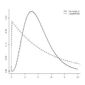
(a) $\gamma(4,1)$

(b) $\mathcal{L}\gamma(2,1)$

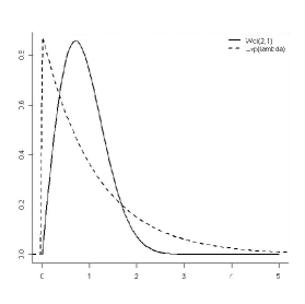
(c) $Wei(2,1)$

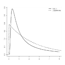
(d) $IG(4,1)$

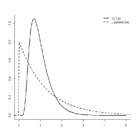
(e) $IG(1,4)$

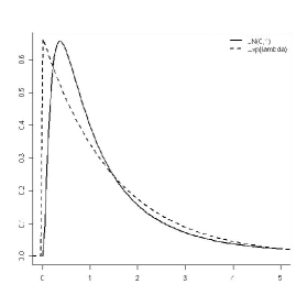
(f) $\mathcal{LN}(0,1)$

Figure 1: Densities of some alternative distributions compared with the density of a fitted exponential distribution. Parameter estimation is based on a sample from the corresponding alternative with $n=100$ and $r=75$.

Simulation results for testing the hypothesis of exponentiality are given in Tables 2 and 3. The conclusions drawn from these results are as follows:

Level:

Most procedures maintain the nominal level very well, with the tests based on the MS and FK2 transforms being somewhat conservative.

$\gamma(\alpha,\beta)$ and $\mathcal{L}\gamma(\alpha,\beta)$ alternatives:

(Figure 1(a)(b)) Due to the similarity of the gamma to the exponential distribution, detecting this hypothesis is difficult. In fact, transformations MS, OS and FK2 seem completely unsuitable for this purpose. On the other hand, the tests based on the LHB transformation seem to work best against gamma alternatives, while against logarithmic gamma alternatives, the tests based on MS and OS are also competitive.

For the $\mathcal{L}\gamma(2,1)$ distribution, all tests based on the LHB transformation show an astonishing behaviour: The power is sharply decreasing when $r$ is increasing, i.e. with a lower degree of censoring. The same can be seen for further alternatives. This behaviour of the LHB transform can also be observed when testing a simple hypotheses, see Tables I-IV in Lin et al. (2008): there, the power of the Anderson-Darling test combined with the LHB transform, called ${}_{\stackrel{{\scriptstyle\ast}}{{T}}}A_{r}^{2}$, decreases with $r$ for several alternatives (in particular for alternatives $F_{41}$ and $F_{51}$ which are defined on p. 634 in Lin et al. (2008)). Similar patterns also occur with other transformations, see the results for the Anderson-Darling test combined with the MS transform, called ${}_{T}A_{r}^{2}$, in Lin et al. (2008), and Table 1 in O’Reilly and Stephens (1988) for tests based on the OS transformation.

$Wei(\alpha,\beta)$ alternatives:

(Figure 1(c)) Again, tests based on the LHB transform are the best, followed by FK1, while the tests based on the FK2 transformation is clearly unable to detect the Weibull alternatives used in the simulations.

$IG(\mu,\lambda)$ and $\mathcal{LN}(\mu,\sigma)$ alternatives:

(Figure 1(d)(e)(f)) For these distributions, the tests based on FK1 and FK2 do not work. Interestingly, the MS and OS–based tests work much better against $IG(4,1)$ than LHB, while the converse holds true for the $IG(1,4)$ distribution. The power results against the $\mathcal{LN}(0,1)$ distribution comply with the fact that this distribution is hard to distinguish from a suitable exponential distribution (see Figure 1(d)).

Summary:

The tests based on the transformation of Lin, Huang and Balakrishnan should be used, while the tests based on FK1 and FK2 do not work well. Also within one transformation, the difference between the four test statistics is not always particularly noticeable. Nevertheless, in many cases the characteristic function based test has slightly higher power than the tests based on the empirical distribution function.

In the simulations for the exponential distribution, we added results for the two most common direct statistics (DS), i.e., statistics which are modifications of corresponding full–sample versions and may be applied directly to the original censored data, without transformations. These tests are the Cramér-von Mises and the Anderson-Darling test; see Section 4.9.5 of D’Agostino, Stephens (1986). Corresponding results are given in obvious notation in the last two columns in Tables 2 and 3. Generally, the newly proposed tests have inferior power. Recall however their advantage of general applicability: We do not need new critical values for each distribution, sample size and censoring proportion, not to mention dependence on parameters and corresponding estimators. In this connection note that since even for this standard distribution critical values for our censoring proportions 25% and 50% are not available in the literature, they are provided in Table 1.

$n$	$\frac{r}{n}$	$A^{2}_{r,n}$			$W^{2}_{r,n}$
		$10\%$	$5\%$	$1\%$	$10\%$	$5\%$	$1\%$
40	0.50	0.479	0.609	0.932	0.063	0.081	0.124
40	0.75	0.726	0.918	1.401	0.12	0.152	0.232
100	0.50	0.483	0.617	0.953	0.063	0.082	0.127
100	0.75	0.734	0.930	1.414	0.121	0.154	0.237

Table 1: Critical values of direct edf statistics for testing for exponentiality based on $10^{7}$ replications

Distribution	$\frac{r}{n}*100\%$	$n$	MS			OS			LHB			FK1			FK2			DS
			$A^{2}$	$W^{2}$	$C^{2}$	$A^{2}$	$W^{2}$	$C^{2}$	$A^{2}$	$W^{2}$	$C^{2}$	$A^{2}$	$W^{2}$	$C^{2}$	$A^{2}$	$W^{2}$	$C^{2}$	$A^{2}_{r,n}$	$W^{2}_{r,n}$
$Exp(1)$	50	40	4	4	3	6	6	5	5	5	4	5	5	4	4	4	3	5	5
	50	100	4	4	3	5	5	5	5	5	5	5	5	4	4	4	3	4	4
	75	40	4	4	4	5	5	5	5	5	5	5	5	5	4	4	4	5	5
	75	100	4	5	4	6	5	6	5	5	5	5	5	5	4	4	4	5	5
$\gamma(2,1)$	50	40	4	4	3	6	6	6	7	6	7	7	6	6	0	0	0	53	53
	50	100	4	4	4	6	6	6	12	11	15	12	9	14	0	0	1	95	92
	75	40	5	4	4	6	5	6	8	8	9	8	7	8	0	0	0	70	68
	75	100	6	5	5	6	6	6	17	14	20	16	13	19	0	1	1	99	98
$\gamma(4,1)$	50	40	5	5	3	7	6	6	28	24	33	7	6	7	0	0	0	99	99
	50	100	6	5	4	6	6	6	74	63	80	15	10	18	0	0	0	100	100
	75	40	5	5	4	6	6	6	42	34	49	9	7	10	0	0	0	100	100
	75	100	7	6	6	5	5	5	89	80	93	23	16	29	0	0	0	100	100
$IG(4,1)$	50	40	15	14	15	13	12	11	5	5	5	4	3	4	2	2	2	19	16
	50	100	36	32	41	38	34	42	10	9	12	5	4	4	4	5	6	62	37
	75	40	39	35	43	36	33	39	6	6	6	5	4	5	15	14	17	23	26
	75	100	79	72	83	86	80	89	13	12	15	7	5	6	36	32	44	64	58
$IG(1,4)$	50	40	5	5	3	6	6	5	59	48	67	3	2	3	0	0	0	100	100
	50	100	11	10	9	10	9	10	99	94	99	7	5	10	0	0	0	100	100
	75	40	8	8	6	8	7	7	74	61	82	5	3	6	0	0	0	100	100
	75	100	18	16	18	16	15	18	100	99	100	12	7	17	0	0	1	100	100

Table 2: Percentage of rejection of tests for exponentiality based on 10000 replications (part 1)

Distribution	$\frac{r}{n}*100\%$	$n$	MS			OS			LHB			FK1			FK2			DS
			$A^{2}$	$W^{2}$	$C^{2}$	$A^{2}$	$W^{2}$	$C^{2}$	$A^{2}$	$W^{2}$	$C^{2}$	$A^{2}$	$W^{2}$	$C^{2}$	$A^{2}$	$W^{2}$	$C^{2}$	$A^{2}_{r,n}$	$W^{2}_{r,n}$
$Wei(2,1)$	50	40	5	5	4	10	9	10	12	11	14	8	7	8	0	0	0	84	85
	50	100	5	5	5	12	11	13	30	25	36	19	14	21	0	0	0	100	100
	75	40	8	7	7	12	11	13	20	17	23	12	10	13	0	0	0	98	98
	75	100	10	8	11	17	15	21	50	41	56	30	22	35	0	0	0	100	100
$Wei(4,1)$	50	40	11	10	10	14	13	15	65	57	72	7	5	7	0	0	0	100	100
	50	100	15	12	14	18	16	21	99	97	99	21	14	27	0	0	0	100	100
	75	40	20	17	20	19	17	21	88	81	92	11	8	14	0	0	0	100	100
	75	100	41	31	43	31	28	36	100	100	100	40	28	51	0	0	0	100	100
$\mathcal{L}\gamma(2,1)$	50	40	30	27	31	29	26	28	19	16	23	2	2	2	1	1	2	73	61
	50	100	75	67	77	80	73	82	73	52	80	2	1	2	5	6	12	100	99
	75	40	71	65	73	70	64	71	16	14	19	3	2	3	20	19	26	55	46
	75	100	99	97	99	100	99	99	50	40	57	5	4	6	57	51	69	100	93
$\mathcal{L}\gamma(4,1)$	50	40	22	20	24	19	17	18	6	5	5	4	3	3	8	8	8	13	15
	50	100	51	45	57	58	51	63	8	8	9	6	5	5	16	16	20	32	33
	75	40	58	51	63	57	52	60	19	17	20	5	4	5	48	44	47	76	78
	75	100	93	87	94	97	95	98	37	34	42	11	9	11	82	76	84	98	99
$\mathcal{LN}(0,1)$	50	40	6	6	5	6	6	4	5	5	5	6	4	5	0	1	1	34	32
	50	100	12	11	12	10	10	10	10	8	12	7	5	8	1	1	2	84	70
	75	40	11	10	12	9	9	9	5	5	5	6	5	6	2	2	2	26	22
	75	100	26	23	30	25	23	28	8	8	10	7	5	7	3	4	5	73	53

Table 3: Percentage of rejection of tests for exponentiality based on 10000 replications (part 2)

5.2 Testing for gamma distribution

Simulation results for testing the gamma hypothesis are given in Tables 4 and 5. The conclusions drawn from these results are as follows:

(a) $\mathcal{L}\gamma(2,1)$

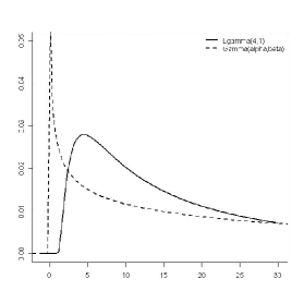
(b) $\mathcal{L}\gamma(4,1)$

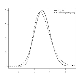
(c) $\mathcal{N}(3,1)$

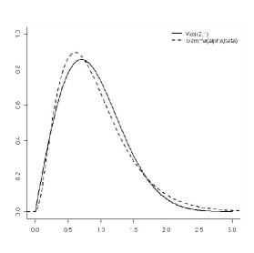
(d) $Wei(2,1)$

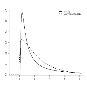
(e) $IG(4,1)$

(f) $IG(1,4)$

Figure 2: Densities of some alternative distributions compared with the density of a fitted gamma distribution. Parameter estimation is based on a sample from the corresponding alternative with $n=100$ and $r=75$.

Level:

The tests based on the OS and LHB transformations maintain the nominal level very well, while those based on the MS, FK1 and FK2 are somewhat conservative.

$\mathcal{L}\gamma(\alpha,\beta)$ alternatives:

(Figure 2(a),(b)) All variants of MS and OS based tests have good power against the logarithmic gamma distribution, while the FK1–based tests are worst in this case.

$\mathcal{N}(3,1)$ alternative:

(Figure 2(c)) The tests based on the MS and the OS transformation (in this order) have higher powers against the $\mathcal{N}(3,1)$ distribution.

$Wei(\alpha,\beta)$ alternatives:

(Figure 2(d)) Given the fact that Weibull distributions can be approximated quite well by suitable gamma distributions it is not suprising to see that power is low, uniformly over all tests and transformations. Clearly however the OS–based tests stand out as best.

$IG(\mu,\lambda)$ and $\mathcal{LN}(\mu,\sigma)$ alternatives:

(Figure 2(e),(f)) The $\mathcal{LN}(0,1)$ and the $IG(1,4)$ distributions can be well fitted by a gamma distribution. Hence, power against these alternatives is generally low. Against the $IG(4,1)$ alternative the tests based on MS and OS work best.

Summary:

Several of the alternatives are difficult to distinguish from a fitted gamma distribution. The best results are observed with the tests based on the transformations of Michael and Schucany and O’Reilly and Stephens, and within these transformations the test based on the characteristic function have a certain edge.

Distribution	$\frac{r}{n}*100\%$	$n$	MS			OS			LHB			FK1			FK2
			$A^{2}$	$W^{2}$	$C^{2}$	$A^{2}$	$W^{2}$	$C^{2}$	$A^{2}$	$W^{2}$	$C^{2}$	$A^{2}$	$W^{2}$	$C^{2}$	$A^{2}$	$W^{2}$	$C^{2}$
$\gamma(2,1)$	50	40	4	4	3	6	6	5	5	5	4	3	4	3	3	4	3
	50	100	4	4	4	6	6	6	5	5	5	4	4	4	4	4	4
	75	40	4	4	4	6	6	5	5	5	5	4	4	3	4	4	4
	75	100	5	5	4	6	6	6	5	5	5	4	5	4	4	5	4
$\mathcal{N}(3,1)$	50	40	16	15	17	25	23	26	10	10	9	9	9	9	9	9	8
	50	100	31	28	34	46	42	49	17	17	17	19	18	19	18	17	19
	75	40	22	20	24	31	28	34	10	10	10	11	10	11	10	10	11
	75	100	41	38	46	56	52	61	18	17	18	22	19	21	21	19	22
$\mathcal{LN}(0,1)$	50	40	6	6	6	5	5	4	5	5	4	4	4	3	4	5	4
	50	100	9	9	10	9	8	9	5	5	5	4	4	4	5	6	6
	75	40	11	11	12	9	9	9	5	5	5	4	4	4	6	6	7
	75	100	22	20	26	24	22	27	5	5	5	5	5	5	10	10	12
$IG(4,1)$	50	40	15	14	16	12	11	11	4	5	4	4	4	3	6	7	6
	50	100	32	29	37	37	32	41	6	6	6	5	5	5	12	12	14
	75	40	39	35	44	37	33	39	6	6	6	5	4	4	15	14	17
	75	100	77	70	81	85	80	88	11	10	13	7	6	7	38	35	47
$IG(1,4)$	50	40	5	5	4	4	4	3	5	5	5	3	4	3	4	4	3
	50	100	6	6	7	6	6	6	6	5	5	4	4	4	5	5	5
	75	40	7	7	7	6	6	5	5	5	5	4	4	4	5	6	5
	75	100	11	11	13	11	10	12	5	5	5	5	4	4	7	7	8

Table 4: Percentage of rejection of tests for gamma distribution based on 10000 replications (part 1)

Distribution	$\frac{r}{n}*100\%$	$n$	MS			OS			LHB			FK1			FK2
			$A^{2}$	$W^{2}$	$C^{2}$	$A^{2}$	$W^{2}$	$C^{2}$	$A^{2}$	$W^{2}$	$C^{2}$	$A^{2}$	$W^{2}$	$C^{2}$	$A^{2}$	$W^{2}$	$C^{2}$
$Wei(2,1)$	50	40	4	5	4	9	8	9	5	5	4	3	4	3	3	4	3
	50	100	5	6	6	13	11	14	5	5	5	5	5	4	4	5	4
	75	40	6	6	7	12	10	13	5	5	4	4	5	4	4	4	4
	75	100	9	8	10	18	16	21	5	5	5	4	5	4	5	6	6
$Wei(4,1)$	50	40	7	7	7	14	13	14	5	5	4	4	4	3	4	4	4
	50	100	9	8	10	22	19	24	5	5	5	4	5	4	5	5	6
	75	40	11	10	12	20	18	22	5	5	5	4	5	4	5	5	6
	75	100	20	18	23	37	32	43	5	5	5	6	6	5	8	8	10
$\mathcal{L}\gamma(2,1)$	50	40	30	27	33	26	23	25	5	6	5	4	4	3	11	11	12
	50	100	70	62	73	77	69	79	12	11	13	7	5	6	29	26	36
	75	40	71	64	73	70	63	71	12	11	13	4	3	4	32	29	37
	75	100	98	95	98	99	99	99	36	31	42	8	6	8	77	69	84
$\mathcal{L}\gamma(4,1)$	50	40	22	19	24	18	16	18	5	5	4	4	3	3	7	7	8
	50	100	51	45	57	58	52	63	8	7	8	6	5	5	17	17	22
	75	40	58	52	62	57	51	60	9	9	10	4	3	4	20	19	24
	75	100	94	89	95	98	96	98	25	22	29	6	5	6	54	47	63

Table 5: Percentage of rejection of tests for gamma distribution based on 10000 replications (part 2)

5.3 Testing for normality

Simulation results for testing the hypothesis of normality using the estimates suggested by Gupta (1952) are given in Tables 7 and 8. The conclusions drawn from these results are as follows:

(a) $IG(4,1)$

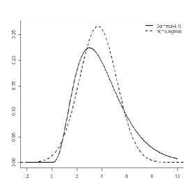
(b) $\gamma(4,1)$

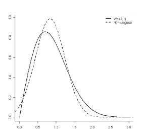
(c) $Wei(2,1)$

Figure 3: Densities of some alternative distributions compared with the density of a fitted normal distribution. Parameter estimation is based on a sample from the corresponding alternative with $n=100$ and $r=75$.

Level

: Apart from the tests based on FK1, which are somewhat conservative, all tests maintain the nominal level very well.

$IG(\mu,\lambda)$ and $\mathcal{LN}(\mu,\sigma)$ alternatives:

(Figure 3(a)) For these alternatives, the MS, OS and FK2–based tests have higher powers than LIN and FK1-based tests.

$t_{m}$ alternatives:

The tests based on MS and OS transforms give the best results, with powers being significantly lower for the $t_{4}$ alternative.

$Exp(\lambda)$ alternative:

The tests based on the MS, OS and FK2 transformations detect this alternative reliably for medium and low censoring ($r\geq n/2)$ and are clearly preferable to tests based on LHB and FK1.

$\gamma(\alpha,\beta)$ and $\mathcal{L}\gamma(\alpha,\beta)$ alternatives:

(Figure 3(b)) The tests based on MS, OS and FK2 transformation have high power against logarithmic gamma distributions for medium and low censoring. They are also preferable against gamma alternatives.

$Wei(\alpha,\beta)$ alternatives:

(Figure 3(c)) Due to the similarity of the $Wei(3,1)$ and $Wei(3,5)$ and suitable normal densities, power is only slightly above the nominal level.

$\mathcal{L}(\alpha,\beta)$ alternatives:

Again, this alternative is hard to distinguish from a normal distribution. Nevertheless, MS and OS based tests show some power.

Summary:

The highest power is observed with the tests based on the transformations of Michael and Schucany and O’Reilly and Stephens. However, the tests based on transformation FK2 also show a comparable behavior.

As in the case of the exponential distribution, we added results for the direct statistics (DS), the Cramér-von Mises and the Anderson-Darling test; see Section 4.8.4 of D’Agostino and Stephens (1986) for the normal distribution with censored data. Corresponding results are given in the last two columns in Tables 7 and 8. Critical values for our censoring proportions 25% and 50% and sample sizes $n=40$ and $100$ are provided in Table 6. All comments given at the end of section 5.1 for the exponential case also apply here, although the transformed–based tests are more competitive in this case.

$n$	$\frac{r}{n}$	$A^{2}_{r,n}$			$W^{2}_{r,n}$
		$10\%$	$5\%$	$1\%$	$10\%$	$5\%$	$1\%$
40	0.50	0.222	0.286	0.493	0.036	0.049	0.097
40	0.75	0.364	0.451	0.683	0.064	0.080	0.120
100	0.50	0.227	0.285	0.446	0.036	0.047	0.083
100	0.75	0.369	0.453	0.662	0.066	0.081	0.120

Table 6: Critical values of direct edf statistics for testing for normality based on $10^{7}$ replications

We repeated the simulations using modified maximum likelihood estimation as suggested by Tiku (1967). The results have been quite similar but power was slightly worse compared to the method of Gupta. Therefore, the results have been omitted.

Distribution	$\frac{r}{n}*100\%$	$n$	MS			OS			LHB			FK1			FK2			DS
			$A^{2}$	$W^{2}$	$C^{2}$	$A^{2}$	$W^{2}$	$C^{2}$	$A^{2}$	$W^{2}$	$C^{2}$	$A^{2}$	$W^{2}$	$C^{2}$	$A^{2}$	$W^{2}$	$C^{2}$	$A^{2}_{r,n}$	$W^{2}_{r,n}$
$\mathcal{N}(0,1)$	50	40	6	5	5	6	5	5	5	5	5	3	3	3	5	5	5	5	5
	50	100	5	5	5	6	6	6	5	5	5	4	4	3	5	5	5	5	5
	75	40	6	5	6	6	6	6	5	5	5	4	4	3	5	5	5	5	5
	75	100	5	5	5	6	5	5	5	5	4	4	4	3	5	5	5	5	5
$\mathcal{LN}(0,1)$	50	40	50	44	53	33	30	32	9	8	10	9	8	8	42	39	41	65	66
	50	100	87	78	87	85	78	86	19	18	21	15	12	13	81	76	83	98	98
	75	40	85	79	85	79	73	79	20	19	22	12	9	11	76	72	78	94	92
	75	100	100	99	100	100	100	100	55	52	61	21	15	17	99	99	99	100	100
$IG(4,1)$	50	40	75	70	77	60	55	58	16	14	17	12	9	11	65	61	64	88	88
	50	100	99	97	99	99	97	99	45	43	49	21	15	17	98	96	98	100	100
	75	40	99	98	98	98	96	97	49	47	52	20	14	18	96	95	97	100	100
	75	100	100	100	100	100	100	100	93	92	95	29	20	23	100	100	100	100	100
$IG(1,4)$	50	40	18	16	19	9	9	8	6	6	6	6	5	5	16	15	16	28	30
	50	100	33	28	37	28	25	31	7	6	7	9	8	7	32	28	33	59	62
	75	40	34	30	38	25	23	27	6	6	7	8	6	7	29	26	30	49	46
	75	100	66	56	69	69	62	74	10	10	12	12	10	10	59	53	64	89	87
$t_{2}$	50	40	50	47	52	58	55	60	10	10	11	2	2	1	5	4	7	37	27
	50	100	82	78	84	88	86	90	24	22	26	25	15	24	14	8	20	79	74
	75	40	56	53	59	61	58	64	13	12	14	17	11	16	7	5	9	53	51
	75	100	87	85	89	90	88	91	33	29	35	47	33	45	19	11	21	88	87
$t_{4}$	50	40	20	18	22	26	23	28	6	6	5	3	3	2	4	4	4	13	8
	50	100	37	32	40	46	41	50	7	6	7	6	5	6	6	5	9	35	28
	75	40	23	20	25	27	25	30	5	5	5	5	4	5	4	4	5	20	18
	75	100	41	36	44	47	42	51	9	8	9	11	7	11	8	6	9	44	41

Table 7: Percentage of rejection of tests for normality based on 10000 replications (part 1)

Distribution	$\frac{r}{n}*100\%$	$n$	MS			OS			LHB			FK1			FK2			DS
			$A^{2}$	$W^{2}$	$C^{2}$	$A^{2}$	$W^{2}$	$C^{2}$	$A^{2}$	$W^{2}$	$C^{2}$	$A^{2}$	$W^{2}$	$C^{2}$	$A^{2}$	$W^{2}$	$C^{2}$	$A^{2}_{r,n}$	$W^{2}_{r,n}$
$\mathcal{L}(0,1)$	50	40	9	9	10	13	12	14	5	5	5	3	3	2	4	4	4	5	4
	50	100	13	11	15	20	17	22	5	5	5	4	4	3	5	5	6	11	8
	75	40	11	10	11	13	11	15	5	5	5	4	4	3	4	4	5	8	7
	75	100	15	13	17	19	16	22	5	5	5	4	4	4	5	5	6	16	14
$Wei(2,1)$	50	40	14	12	14	8	7	6	5	5	5	5	5	4	13	12	12	20	22
	50	100	24	20	27	20	17	22	6	6	6	8	7	7	24	21	26	46	48
	75	40	17	14	18	12	11	11	5	5	5	6	6	5	15	14	16	27	24
	75	100	33	26	36	34	29	38	6	6	6	8	8	8	29	26	33	59	53
$Exp(1)$	50	40	61	53	60	44	39	40	10	9	10	10	8	8	57	53	57	78	77
	50	100	95	90	94	95	90	94	26	25	30	22	19	19	95	92	96	100	100
	75	40	83	75	81	77	70	74	16	15	17	12	9	10	78	74	80	94	91
	75	100	100	99	99	100	99	100	49	45	55	27	22	25	100	99	100	100	100
$\gamma(2,1)$	50	40	27	23	29	15	14	13	6	6	6	7	6	5	23	22	23	40	42
	50	100	55	45	58	51	43	54	9	8	10	12	11	10	52	46	55	82	83
	75	40	45	38	47	35	30	36	7	7	7	9	7	7	37	35	40	62	57
	75	100	82	71	83	86	78	88	15	14	17	14	12	12	76	70	80	97	95
$\gamma(4,1)$	50	40	14	12	15	7	7	5	6	6	5	6	6	5	13	13	13	20	22
	50	100	23	19	26	19	16	20	6	6	6	8	7	6	22	20	23	44	47
	75	40	22	19	24	15	14	15	6	6	6	7	6	5	18	17	19	32	30
	75	100	42	35	47	44	38	50	7	6	7	10	8	9	37	33	41	68	64
$\mathcal{L}\gamma(2,1)$	50	40	80	74	81	66	61	64	19	17	21	13	10	12	72	68	71	90	90
	50	100	99	98	99	99	98	99	51	49	56	23	17	18	99	98	99	100	100
	75	40	99	99	99	99	98	99	60	58	63	23	17	23	98	97	98	100	100
	75	100	100	100	100	100	100	100	97	96	98	32	23	28	100	100	100	100	100

Table 8: Percentage of rejection of tests for normality based on 10000 replications (part 2)

5.4 Summary of simulation results

In this subsection, we try to convey a qualitative message based on the simulation results. Table 9 has the three tests as entries for the lines, and the five transformations to uniformity as entries for the columns. At each cell, i.e. at each specific combination of test and transformation, there are two entries which show order: The left digit is the order w.r.t. the lines (tests), while the right digit shows the order w.r.t. the columns (transformations). For example the entry $2\backslash 1$ in the first cell means that the Anderson-Darling test is the second best for the MS transformation, while the MS transformation ranks 1st for the Anderson-Darling test.

To get such an overall assessment for, say, a fixed transformation, we assigned ranks to the three tests. The test with the highest percentage of rejection has rank one, and so on. Then, we summed up the ranks for all listed combinations of null hypotheses, alternatives and censoring proportions $r$. The test with the lowest sum score has the entry 1 in Table 9 for this transformation.

This overview gives a clear picture: For any given test, the MS and OS transformations perform best. In this connection, a direct look at the sum scores shows that there is not much to choose between these two transforms. On the other hand, the LHB transform follows at a clear distance, having the edge over FK2. By far the lowest sum score for all tests has the FK1 transformation. Also, for the MS and OS transformations, the best test is the characteristic function test $C^{2}$. $C^{2}$ also performs best for LHB and FK2 transform. Finally, the best combination of test and transformation is $C^{2}$ with OS.

	MS	OS	LHB	FK1	FK2
$A^{2}$
$W^{2}$
$C^{2}$

Table 9: Overall assessment for the tests and transformations. Left digit: order w.r.t. the lines (tests). Right digit: order w.r.t. the columns (transformations).

6 Conclusion

We have applied a series of transformations to original type–II censored data with the aim of rendering corresponding full–sample tests statistics for the parent population, applicable and approximately distribution–free. The conclusions from our Monte Carlo study show that these transformations generally work well across all goodness–of–fit tests studied in terms of recovering the nominal level of significance. On the other hand, the best transformation in terms of power depends on the distribution under test, with the transformation of Lin et al. (2008) being best for testing exponentiality, and the transformations of Michael and Schucany (1988) and O’Reilly and Stephens (1988) for testing normality and testing for the gamma distribution. Also, and within each transformation, the characteristic function based test seem to yield the best power for the majority of alternatives. However, this superiority is generally not significant compared to the large differences between the transformations. Before closing however we wish to reiterate once more that, despite the fact that the transformed based tests often show good power, their advantage lies not so much in the power but in the general applicability of the method: The user does not need new critical values for each distribution under test, each combination of sample size and censoring proportion, and each possible choice of parameter value/parameter estimate, but, following the transformation suggested, essentially faces the simplified problem of testing for normality with estimated parameters.

Appendix A Appendix

In this appendix we shall investigate the reasons underlying the eventual validity of the Chen–Balakrishnan transformation. In doing so, first in Appendix A.1 we report results on the process corresponding to goodness–of–fit testing for the normal distribution with estimated parameters. Then in Appendices A.2 and A.3 we study in detail the process produced by the Chen–Balakrishnan transformation and compare it with the process in A.1 both theoretically and by simulation.

A.1 The empirical process under normality

Suppose that $Z_{j},\ j=1,...,n$, are iid normal with unknown mean and variance. Then most standard goodness–of–fit tests are merely functionals of the empirical process

$$\hat{\alpha}_{n}(t) = \frac{1}{\sqrt{n}}\sum_{j}\left[I\left\{\Phi\left(\frac{Z_{j}-\bar{Z}}{s_{Z}}\right)\leq t\right\}-t\right]$$

$$= \frac{1}{\sqrt{n}}\sum_{j}\left[I\left\{U_{j}\leq\Phi\left(\bar{Z}+s_{Z}\;\Phi^{-1}(t)\right)\right\}-t\right],$$

where $\bar{Z}$ and $s_{Z}$ are the sample mean and sample variance of $Z_{1},...,Z_{n}$, and $U_{j}=\Phi(Z_{j})$ and $t\in[0,1]$. This process has been studied by Durbin (1973) and showed that under regularity conditions,

$$\hat{\alpha}_{n}\Rightarrow\alpha$$

where $\alpha$ is a centered Gaussian process with covariance function

$$C(\alpha(s),\alpha(t)) = \min(s,t)-st-\varphi(\Phi^{-1}(s))\varphi(\Phi^{-1}(s))$$

$$-\frac{1}{2}\Phi^{-1}(s)\varphi(\Phi^{-1}(s))\Phi^{-1}(t)\varphi(\Phi^{-1}(t)),$$

where $\Phi^{-1}$ and $\varphi$ are the quantile and density function of the standard normal distribution. (We note that Loynes (1980) extended the analysis from the iid setting to the case of generalized linear models). Clearly the process $\alpha_{n}$ is identical to the process involved in the Chen–Balakrishnan transformation only in the case of testing for normality with estimated parameters.

A.2 The empirical process under non–normality

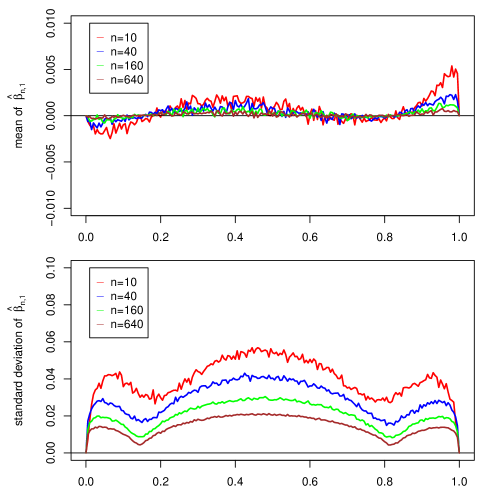
Figure 4: Simulated mean and standard deviation of $\hat{\beta}_{n,1}$ for different sample sizes

In this section, we consider iid random variables $X_{j}$ with DF ${\cal{F}}_{\vartheta}(x)$ (assumed to be continuous and strictly increasing) and the standardized quantile residuals $Z_{j}=\frac{Y_{j}-\bar{Y}}{s_{Y}}$ with $Y_{j}=\Phi^{-1}\left({\cal{F}}_{\hat{\vartheta}}(X_{j})\right)$ (concerning the term standardized quantile residual, refer to Klar and Meintanis 2011, sec 2.1). We shall study the following empirical process based on the $Z_{j}$:

$$\hat{\beta}_{n}(t) = \frac{1}{\sqrt{n}}\sum_{j}\left[I\left\{\Phi(Z_{j})\leq t\right\}-t\right]$$

$$= \frac{1}{\sqrt{n}}\sum_{j}\left[I\left\{\Phi\left(\frac{Y_{j}-\bar{Y}}{s_{Y}}\right)\leq t\right\}-t\right]$$

$$= \frac{1}{\sqrt{n}}\sum_{j}\left[I\left\{X_{j}\leq{\cal{F}}_{\hat{\vartheta}}^{-1}(\Phi(\bar{Y}+s_{Y}\,\Phi^{-1}(t)))\right\}-t\right]$$

$$= \frac{1}{\sqrt{n}}\sum_{j}\left[I\left\{U_{j}\leq{\cal{F}}_{\vartheta}\left({\cal{F}}_{\hat{\vartheta}}^{-1}\left(\Phi(\bar{Y}+s_{Y}\,\Phi^{-1}(t))\right)\right)\right\}-t\right],$$

where ${\cal{F}}_{\vartheta}^{-1}(p)$ denotes the quantile function of ${\cal{F}}_{\vartheta}(\cdot)$, and $U_{j}={\cal{F}}_{\vartheta}(X_{j})$ are iid uniformly distributed on $[0,1]$. This is the empirical process actually produced by the Chen–Balakrishnan transformation. Now define $c_{Y}(t)=\Phi(\bar{Y}+s_{Y}\Phi^{-1}(t))$, and, similarly, $c_{N}(t)=\Phi(\bar{N}+s_{N}\Phi^{-1}(t))$, where $N_{j}=\Phi^{-1}(U_{j})$ are iid standard normal random variates, and $\bar{N}$ and $s_{N}^{2}$ are the arithmetic mean and sample variance of $N_{1},\ldots,N_{n}$.

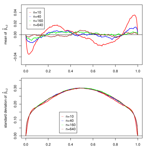
Figure 5: Simulated mean and standard deviation of $\hat{\beta}_{n,2}$ for different sample sizes

Then we can decompose the above process as (compare Chen (1991), pp 126-128)

(A.1) $$\hat{\beta}_{n}(t)=\hat{\beta}_{n,1}(t)+\hat{\beta}_{n,2}(t)+\hat{\beta}_{n,3}(t),$$

where

$$\hat{\beta}_{n,1}(t)=\frac{1}{\sqrt{n}}\sum_{j}\left[I\left\{U_{j}\leq{\cal{F}}_{\vartheta}\left({\cal{F}}_{\hat{\vartheta}}^{-1}(c_{Y}(t))\right)\right\}-{\cal{F}}_{\vartheta}\left({\cal{F}}_{\hat{\vartheta}}^{-1}(c_{Y}(t))\right)\right.\\ -\;I\left\{U_{j}\leq c_{N}(t)\right\}+c_{N}(t){\hbox{$\left]\vbox to0.0pt{}\right.\n@space$}},$$

$$\hat{\beta}_{n,2}(t)=\frac{1}{\sqrt{n}}\sum_{j}\left[I\left\{U_{j}\leq\Phi(\bar{N}+s_{N}\,\Phi^{-1}(t))\right\}-t\right],$$

and

$$\hat{\beta}_{n,3}(t)=\frac{1}{\sqrt{n}}\sum_{j}\left[{\cal{F}}_{\vartheta}\left({\cal{F}}_{\hat{\vartheta}}^{-1}(c_{Y}(t))\right)-c_{N}(t)\right].$$

The first part $\hat{\beta}_{n,1}(t)$ in decomposition (A.1) is the difference of an empirical process and a random perturbation thereof, and should be $o_{P}(1)$ under appropriate regularity conditions (see Chen (1991), p.128, Loynes (1980), Lemma 1, and Rao and Sethuraman (1975)). To check this claim, we simulated a random sample of size $n$ from a unit mean exponential distribution and computed $\hat{\beta}_{n,1}(t),\ t\in[0,1]$, on the basis of an equidistant grid with spacing equal to $0.005$. This was repeated $B=10000$ times. We approximated the mean function $E[\hat{\beta}_{n,1}(t)]$ and the standard deviation $\sqrt{Var[\hat{\beta}_{n,1}(t)]}$ by the arithmetic mean and empirical standard deviation based on the $B$ replications; Figure 4 shows the result for sample sizes $n=10,40,160$ and $640$. Clearly the mean function is nearly zero and decreases for increasing $n$, while the standard deviation is small compared to the standard deviation of $\hat{\beta}_{n}$ or $\hat{\beta}_{n,2}$ (see below). The corresponding variance seems to converge to zero, but rather slowly, with a speed of convergence approximately equal to $1/\sqrt{n}$.

The second part $\hat{\beta}_{n,2}$ corresponds to the normal empirical process $\hat{\alpha}_{n}$ in Appendix A.1. Figure 5 shows the empirical mean function and standard deviation of $\hat{\beta}_{n,2}$ for an underlying exponential distribution computed in the same way as for $\hat{\beta}_{n,1}$ above. The mean function, which takes on much larger values than that of $\hat{\beta}_{n,1}$, again converges to zero, whereas the variance function is nearly constant for $n\geq 40$.

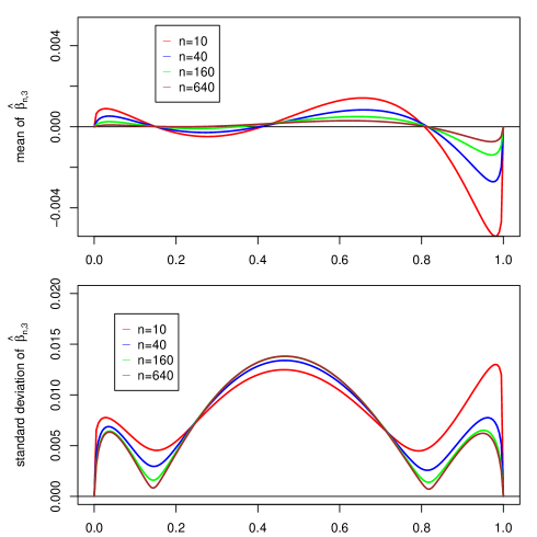
Figure 6: Simulated mean and standard deviation of $\hat{\beta}_{n,3}$ for different sample sizes

For the third part we have

$$\hat{\beta}_{n,3}(t)=\sqrt{n}\left[{\cal{F}}_{\vartheta}\left({\cal{F}}_{\hat{\vartheta}}^{-1}(\Phi(\bar{Y}+s_{Y}\,\Phi^{-1}(t)))\right)-\Phi(\bar{N}+s_{N}\,\Phi^{-1}(t))\right].$$

In general, this process does not converge to zero in probability. However, the contribution of $\hat{\beta}_{n,3}$ seems to be negligibly small in comparison to $\hat{\beta}_{n,2}$ in many situations. Figure 6 shows the empirical mean function and standard deviation of $\hat{\beta}_{n,3}$ for the exponential distribution, computed as above. The mean function is very small and goes to zero. The standard deviation is small compared to the standard deviation of $\hat{\beta}_{n,2}$, and it converges, but not to zero. We stress that the crucial point for the behavior of $\hat{\beta}_{n,3}$ is the coupling between the $Y_{j}$’s and the normal variates $N_{j}$ which are both based on the original $X_{j}$, the first computed by using $\hat{\vartheta}$ while the second by using $\vartheta$. In fact if we generate iid standard normal random variables $\tilde{N}_{j}$ independent of the $X_{j}$’s and use them instead of the $N_{j}$’s, the mean function is small, but does not seem to converge to zero, and the variance is much larger, even larger than that of $\hat{\beta}_{n,2}$.

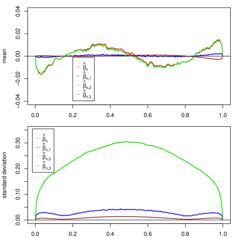
Figure 7: Simulated mean and standard deviation of the different processes for sample size $n=40$

From the above it follows that the values of the process $\hat{\beta}_{n}$ will be eventually dominated by $\hat{\beta}_{n,2}$, at least for large $n$. This is documented in Figure 7 where the mean and standard deviation of all four processes are plotted for $n=40$. Note that the standard deviations of $\hat{\beta}_{n}$ (in red) and $\hat{\beta}_{n,2}$ (in green) are nearly identical, and therefore, visually indistinguishable.

A.3 Further analysis of the process $\boldsymbol{\hat{\beta}_{n,3}}$

To keep things simple, we assume in the following that $\vartheta\in\Theta\subset{\rm I\kern-1.79997ptR}$. Let $\vartheta_{0}$ denote the true parameter value, and define

$$N_{j}(\vartheta) = \Phi^{-1}\left({\cal{F}}_{\vartheta}\left(X_{j}\right)\right),$$

$$\bar{N}(\vartheta) = \frac{1}{n}\sum_{j=1}^{n}N_{j}(\vartheta),\quad s_{N}^{2}(\vartheta)\;=\;\frac{1}{n-1}\sum_{j=1}^{n}\left(N_{j}(\vartheta)-\bar{N}(\vartheta)\right)^{2}.$$

Then, $N_{j}(\vartheta_{0})=N_{j},\bar{N}(\vartheta_{0})=\bar{N},s_{N}^{2}(\vartheta_{0})=s_{N}^{2}$, and $N_{j}(\hat{\vartheta})=Y_{j},\bar{N}(\hat{\vartheta})=\bar{Y},s_{N}^{2}(\hat{\vartheta})=s_{Y}^{2}$. Putting

$$h_{t}(\vartheta) = \Phi\left(\bar{N}(\vartheta)+s_{N}(\vartheta)\cdot\Phi^{-1}(t)\right),$$

we obtain $h_{t}(\vartheta_{0})=c_{N}(t)$ and $h_{t}(\hat{\vartheta})=c_{Y}(t)$. Thus, we can write

(A.2) $$\hat{\beta}_{n,3}(t) = \sqrt{n}\left(g_{t}(\hat{\vartheta})-g_{t}(\vartheta_{0})\right),$$

where

$$g_{t}(\vartheta) = {\cal{F}}_{\vartheta_{0}}\left({\cal{F}}_{\vartheta}^{-1}\left(h_{t}(\vartheta)\right)\right).$$

Assume now that $\sqrt{n}(\hat{\vartheta}-\vartheta_{0})=O_{p}(1)$. Then, by using the expansion

$$g_{t}(\hat{\vartheta})=g_{t}(\vartheta_{0})+(\hat{\vartheta}-\vartheta_{0})\,g_{t}^{{}^{\prime}}(\vartheta_{0})+(\hat{\vartheta}-\vartheta_{0})^{2}\,g_{t}^{{}^{\prime\prime}}(\vartheta^{*})/2,$$

with $\vartheta^{*}$ between $\hat{\vartheta}$ and $\vartheta_{0}$, and by omitting the quadratic term, we see that $\hat{\beta}_{n,3}(t)$ can be approximated by

(A.3) $$\mathring{\beta}_{n,3}(t) = \sqrt{n}\left(\hat{\vartheta}-\vartheta_{0}\right)\,g_{t}^{{}^{\prime}}\left(\vartheta_{0}\right).$$

Of course, the validity of such a Taylor expansion is not enough to justify the uniform convergence $\sup_{t}|\hat{\beta}_{n,3}(t)-\mathring{\beta}_{n,3}(t)|=o_{P}(1)$. A sufficient condition would be Fréchet differentiability of $g_{t}(\cdot)$ (see, e.g. van der Vaart and Wellner (1996), p. 373). However, since we do not intend to give rigorous theory here, this issue is not discussed in any detail. Further analysis of $g_{t}^{{}^{\prime}}\left(\vartheta_{0}\right)$ leads to the following result, the proof of which is omitted.

Lemma A.1

Let $\bar{W}$ and $s_{W}^{2}$ denote the arithmetic mean and sample variance of the random variables $W_{j0}:=W_{j}(\vartheta_{0})$, with $W_{j}(\vartheta):=dN_{j}(\vartheta)/d\vartheta$, while $r$ denotes the sample correlation coefficient of $W_{10},\ldots,W_{n0}$ and $N_{1},\ldots,N_{n}$. Then,

$$g_{t}^{\prime}(\vartheta_{0}) = \frac{\partial{\cal{F}}_{\vartheta_{0}}\left(F_{\vartheta_{0}}^{-1}(c_{N}(t))\right)}{\partial x}\cdot\left(\frac{\partial{\cal{F}}_{\vartheta_{0}}^{-1}(c_{N}(t))}{\partial p}\cdot h_{t}^{\prime}(\vartheta_{0})+\frac{\partial{\cal{F}}_{\vartheta_{0}}^{-1}(c_{N}(t))}{\partial\vartheta}\right),$$

$$h_{t}^{\prime}(\vartheta_{0}) = \varphi\left(\bar{N}+s_{N}\,\Phi^{-1}(t)\right)\cdot\left(\bar{W}+\Phi^{-1}(t)\,r\,s_{W}\right),$$

where $\varphi(\cdot)$ denotes the density of the standard normal distribution.

Since $N_{1},\ldots,N_{n}$ are iid standard normal variates, $\bar{N}\to 0$ and $s_{N}\to 1$ almost surely. Furthermore, $\bar{W}\to\mu_{W},s_{W}\to\sigma_{W}$, and $r\to\rho$ a.s., where $(\mu_{W},\sigma_{W}^{2})$ are the mean and variance of $W_{10}$, while $\rho$ denotes the correlation coefficient of $W_{10}$ and $N_{1}$. Hence, the following approximation holds for the process in (A.3).

Lemma A.2

The process $\mathring{\beta}_{n,3}(t)$ can be approximated by the process

(A.4) $$\tilde{\beta}_{n,3}(t) = \sqrt{n}\left(\hat{\vartheta}-\vartheta_{0}\right)\,\tilde{g}_{t}^{{}^{\prime}}\left(\vartheta_{0}\right),$$

where

$$\tilde{g}_{t}^{\prime}(\vartheta_{0}) = \frac{\partial{\cal{F}}_{\vartheta_{0}}\left({\cal{F}}_{\vartheta_{0}}^{-1}(t)\right)}{\partial x}\cdot\left(\frac{\partial{\cal{F}}_{\vartheta_{0}}^{-1}(t)}{\partial t}\cdot\tilde{h}_{t}^{\prime}(\vartheta_{0})+\frac{\partial{\cal{F}}_{\vartheta_{0}}^{-1}(t)}{\partial\vartheta}\right),$$

$$\tilde{h}_{t}^{\prime}(\vartheta_{0}) = \varphi\left(\Phi^{-1}(t)\right)\cdot\left(\mu_{W}+\Phi^{-1}(t)\ \rho\ \sigma_{W}\right).$$

Figure 8 shows the simulated mean and standard deviation of $\hat{\beta}_{n,3}$ in (A.2), $\mathring{\beta}_{n,3}$ in (A.3), and $\tilde{\beta}_{n,3}$ in (A.4) for sample size $n=40$ and $n=640$, again for the exponential distribution. The mean functions take on very small values; the standard deviations are very similar in all cases.

Figure 8: Simulated mean and standard deviation of $\hat{\beta}_{n,3}$, $\mathring{\beta}_{n,3}$ and $\tilde{\beta}_{n,3}$ for sample size $n=40$ and $n=640$

Figure 9 shows the function $\tilde{h}_{t}^{\prime}(\vartheta_{0})$, the part inside the brackets in $\tilde{g}_{t}^{\prime}(\vartheta_{0})$, and $\tilde{g}_{t}^{\prime}(\vartheta_{0})$ itself. The values of $\tilde{g}_{t}^{\prime}(\vartheta_{0})$ are close to zero on the whole interval. For this reason, $\hat{\beta}_{n,3}$ is negligible in comparison to $\hat{\beta}_{n,2}$ for the exponential case at hand.

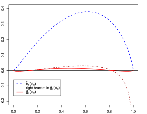
Figure 9: The function $\tilde{h}_{t}^{\prime}(\vartheta_{0})$, the right part of $\tilde{g}_{t}^{\prime}(\vartheta_{0})$, and $\tilde{g}_{t}^{\prime}(\vartheta_{0})$ itself

We also performed Monte Carlo experiments for other gamma distributions with shape parameter not equal to one. These experiments lead to qualitatively similar results and although not reported here they are available from the authors upon request. A reasonable overall conclusion seems to be that under different sampling scenarios the processes $\hat{\beta}_{n,1}$ and $\hat{\beta}_{n,3}$ in decomposition (A.1) are asymptotically negligible, and hence the behavior of the process $\hat{\beta}_{n}$ of the Chen–Balakrishnan transformation is dominated by the values of the process $\hat{\beta}_{n,2}$. The latter process however coincides with the process $\hat{\alpha}_{n}(t)$ of Appendix A.1 which is involved in goodness–of–fit testing for normality with estimated parameters, and this fact justifies the validity of the Chen–Balakrishnan transformation.

References

- \BCAYBesb & MorgBesb & Morg2001 Arcones, M.A. (2006). On the Bahadur slope of the Lilliefors and the Cramér-von Mises tests of normality. In: Gin , Evarist, Koltchinskii, Vladimir, Li, Wenbo, Zinn, Joel (Eds.), IMS Lecture Notes – High Dimensional Probability, vol. 51. pp. 196–206.
- \BCAYBesb & MorgBesb & Morg2001 Bargal, A.I. , & Thomas, D.R. (1983). Smooth goodness of fit tests for the Weibull distribution with singly censored data. Commun. Statist. Theor. Meth., 12, 1431–1447.
- \BCAYBesb & MorgBesb & Morg2001 Baringhaus, L. , Danschke, R. , & Henze, N. (1989). Recent and classical tests for normality. A comparative study. Commun. Statist. Simulation Comput., 18, 363–379.
- \BCAYBesb & MorgBesb & Morg2001 Barr, D.R. , & Davidson, Teddy. (1973). A Kolmogorov–Smirnov test for censored samples. Technometrics, 15, 739–757.
- \BCAYBesb & MorgBesb & Morg2001 Brain, C.W. , & Shapiro, S.S. (1983). A regression test for exponentiality. Technometrics, 25, 69–76.
- \BCAYBesb & MorgBesb & Morg2001 Bowman, A.W., & Foster, P.J. (1993). Adaptive smoothing and density–based tests of multivariate normality. J. Amer. Statist. Assoc., 88, 529–537.
- \BCAYBesb & MorgBesb & Morg2001 Castro–Kuriss, C. (2011). On a goodness–of–fit test for censored data from a location–scale distribution with applications. Chilean J. Statist., 2, 115–136.
- \BCAYMudholkar & HutsonMudholkar & Hutson1996 Castro-Kuriss, C. , Kelmansky, D.M., Leiva, V. , & Martínez, E.J. (2010). On a goodness–of–fit test for normality with unknown parameters and type–II censored data. J. Appl. Statist., 37, 1193–1211.
- \BCAYvan der Vaart & Wellnervan der Vaart & Wellner 1996 Chen, G. (1991). Empirical Processes Based on Regression Residuals: Theory and Applications. Ph.D. Thesis - Simon Fraser University.
- \BCAYBesb & MorgBesb & Morg2001 Chen, G., & Balakrishnan, N. (1995). A general purpose approximate goodness–of–fit test. J. of Quality Technology, 27, 154–161.
- \BCAYD’Agostino & StephensD’Agostino & Stephens1986 D’Agostino, R., & Massaro, J.M. (1992). Goodness-of-fit tests. In: Handbook of the Logistic Distribution. (N. Balakrishnan, Ed.), Marcel Dekker, Inc., New York, 291-371.
- \BCAYD’Agostino & StephensD’Agostino & Stephens1986 D’Agostino, R., & Stephens, M. (1986). Goodness-of-fit techniques. Marcel Dekker, Inc., New York.
- \BCAYBesb & MorgBesb & Morg2001 Dufour, R. , & Maag, U.R. (1978). Distribution results for modified Kolmogorov–Smirnov statistics for truncated or censored samples . Technometrics, 20, 29–32.
- \BCAYBesb & MorgBesb & Morg2001 Durbin, J. (1973). Weak convergence of the sample distribution function when parameters are estimated. Ann. Statist., 1, 279–290.
- \BCAYEppsEpps2005 Epps, T.W. (2005). Tests for location–scale families based on the empirical characteristic function. Metrika, 62, 99–114.
- \BCAYBesb & MorgBesb & Morg2001 Epps, T.W., & Pulley, L.B. (1983). A test for normality based on the empirical characteristic function procedures . Biometrika, 70, 723–726.
- \BCAYBesb & MorgBesb & Morg2001 Fischer, T., & Kamps, U. (2011). On the existence of transformations preserving the structure of order statistics in lower dimensions. J. Statist. Plann. Infer., 141, 536–548.
- \BCAYBesb & MorgBesb & Morg2001 Glen, A.G. , & Foote, B.L. (2009). An inference methodology for life tests with complete samples or type–II right censoring. IEEE Trans. Reliab., 58, 597–603.
- \BCAYBesb & MorgBesb & Morg2001 Grané, A. (2012). Exact goodness–of–fit tests for censored data. Ann. Instit. Statist. Math., 64, 1187–1203.
- \BCAYEppsEpps2005 Gupta, A.K. (1952). Estimation of the mean and standard deviation of a normal population from a censored sample. Biometrika, 39, 266–273.
- \BCAYEppsEpps2005 Henze, N. (1990). An approximation to the limit distribution of the Epps-Pulley test statistic for normality. Metrika, 37, 7–18.
- \BCAYBesb & MorgBesb & Morg2001 Henze, N., & Wagner, T. (1997). A new approach to the BHEP tests for multivariate normality . J. Multivar. Anal. , 62, 1–23.
- \BCAYD’Agostino & StephensD’Agostino & Stephens1986 Klar, B., Meintanis, S.G. (2012). Specification tests for the response distribution in generalized linear models. Computat. Statist., 27, 251–267.
- \BCAYD’Agostino & StephensD’Agostino & Stephens1986 Johnson, N.L., Kotz, S., & Balakrishnan, N. (1994). Continuous Univariate Distributions, Vol. 1. John Wiley & Sons, Inc., New York.
- \BCAYMudholkar & HutsonMudholkar & Hutson1996 Lin, C-T, Huang, Y-L, & Balakrishnan, N. (2008). A new method for goodness–of–fit testing based on Type–II censored samples. IEEE Trans. Reliab., 57, 633–642.
- \BCAYBesb & MorgBesb & Morg2001 Loynes, R.M. (1980). The empirical distribution function of residuals from generalised regression. Ann. Statist., 8, 285–298.
- \BCAYEppsEpps2005 Meintanis, S.G. (2009). Goodness-of-fit testing by transforming to normality: comparison between classical and characteristic function-based methods. J. Statist. Comput. Simul., 79, 205–212.
- \BCAYMudholkar & HutsonMudholkar & Hutson1996 Michael, J.R., & Schucany, W.R. (1988). A new approach to testing goodness of fit for censored samples. Technometrics, 21, 435–441.
- \BCAYMudholkar & HutsonMudholkar & Hutson1996 Mihalko, D.P. , & Moore, D.S. (1980). Chi–square tests of fit for type–II censored data. Ann. Statist. , 8, 625–644.
- \BCAYMudholkar & HutsonMudholkar & Hutson1996 O’Reilly, F.J., & Stephens, M.A. (1988). Transforming censored samples for testing fit. Technometrics, 30, 79–86.
- \BCAYEppsEpps2005 Pettitt, A.N. (1976). Cramér–von Mises statistics for testing normality with censored samples. Biometrika, 63, 475–481.
- \BCAYEppsEpps2005 Pettitt, A.N. (1977). Tests for the exponential distribution with censored data using the Cramér–von Mises statistics. Biometrika, 64, 629–632.
- \BCAYD’Agostino & StephensD’Agostino & Stephens1986 Pea, E.A. (1995). Residuals from Type II Censored Samples In: Recent Advances in Life–Testing and Reliability (N. Balakrishnan, Ed.), CRC Press, London, 523-543.
- \BCAYEppsEpps2005 R Core Team (2012). R: A language and environment for statistical computing. R Foundation for Statistical Computing, Vienna, Austria.
- \BCAYMudholkar & HutsonMudholkar & Hutson1996 Rao, J.S., & Sethuraman, J. (1975). Weak convergence of empirical distribution functions of random variables subject to perturbations and scale factors. Ann. Statist., 3, 299–313.
- \BCAYBesb & MorgBesb & Morg2001 Tenreiro, C. (2009). On the choice of the smoothing parameter for the BHEP goodness–of–fit test. Comput. Statist. Dat. Anal., 53, 1038–1053.
- \BCAYD’Agostino & StephensD’Agostino & Stephens1986 Thode, H.C. (2002). Testing for Normality. Marcel Dekker, Inc., New York.
- \BCAYEppsEpps2005 Tiku, M. L. (1967). Estimating the mean and standard deviation from a censored normal sample. Biometrika, 54, 155–165.
- \BCAYD’Agostino & StephensD’Agostino & Stephens1986 Tiku, M. L., Tan, W. Y., & Balakrishnan, N. (1986). Robust Inference. Marcel Dekker, Inc., New York.
- \BCAYD’Agostino & StephensD’Agostino & Stephens1996 van der Vaart, A.W., &Wellner, J. A. (2002). Weak Convergence and Empirical Processes. Springer, New York.
- \BCAYMudholkar & HutsonMudholkar & Hutson1996 Wilk, M.B., Gnanadesikan, R., & Huyett, M.J. (1962). Estimation of parameters of the gamma distribution using order statistics. Biometrika, 49, 525–545.
- 1