¹³CO Cores in Taurus Molecular Cloud

Abstract

Young stars form in molecular cores, which are dense condensations within molecular clouds. We have searched for molecular cores traced by ¹³CO $J=1\to 0$ emission in the Taurus molecular cloud and studied their properties. Our data set has a spatial dynamic range (the ratio of linear map size to the pixel size) of about 1000 and spectrally resolved velocity information, which together allow a systematic examination of the distribution and dynamic state of ¹³CO cores in a large contiguous region. We use empirical fit to the CO and CO₂ ice to correct for depletion of gas-phase CO. The ¹³CO core mass function (¹³CO CMF) can be fitted better with a log-normal function than with a power law function. We also extract cores and calculate the ¹³CO CMF based on the integrated intensity of ¹³CO and the CMF from 2MASS. We demonstrate that there exists core blending, i.e. combined structures that are incoherent in velocity but continuous in column density.

The core velocity dispersion (CVD), which is the variance of the core velocity difference $\delta v$, exhibits a power-law behavior as a function of the apparent separation $L$:  CVD (km/s) $\propto L({\rm pc})^{0.7}$. This is similar to Larson’s law for the velocity dispersion of the gas. The peak velocities of ¹³CO cores do not deviate from the centroid velocities of the ambient ¹²CO gas by more than half of the line width. The low velocity dispersion among cores, the close similarity between CVD and Larson’s law, and the small separation between core centroid velocities and the ambient gas all suggest that molecular cores condense out of the diffuse gas without additional energy from star formation or significant impact from converging flows.

1 Introduction

Most young stars are found in dense molecular cores (McKee & Ostriker, 2007). There is a large volume of data concerning dense molecular cores traced by dust emission and dust extinction (Motte et al., 1998; Testi & Sargent, 1998; Johnstone et al., 2000; Stanke et al., 2006; Reid & Wilson, 2005, 2006a; Johnstone et al., 2001; Johnstone & Bally, 2006; Alves et al., 2007). One of the primary outcomes of these studies is the core mass function (CMF). Because of the still unknown physical origin of the stellar initial mass function (IMF) and its significance, emphasis has been placed on the possible connection between the CMF and the IMF (Alves et al., 2007).

The construction of an analytic form of the CMF from observational data has largely focused on two functional forms, power law and log-normal. The majority of past studies claim to find a power law CMF, the shape of which resembles the Salpeter IMF (Salpeter, 1955) (The upper mass limit of the original Salpeter IMF is $10M_{\odot}$)

$$\frac{{\rm d}N}{{\rm d}\log M}\propto M^{-\gamma},\ \ \gamma=1.35,-0.4\leq\log(M/M_{\odot})\leq 1.0\>\>.$$ (1)

Such a power law CMF was found in millimeter continuum maps of the $\rho$ Ophiuchus region by Motte et al. (1998) with the IRAM 30-meter telescope and a series of subsequent studies in the Serpens region (Testi & Sargent, 1998), the $\rho$ Ophiuchus region (Johnstone et al., 2000; Stanke et al., 2006), NGC 7538 (Reid & Wilson, 2005), M17 (Reid & Wilson, 2006a), Orion (Johnstone et al., 2001; Johnstone & Bally, 2006) and the Pipe nebula (Alves et al., 2007). Reid & Wilson (2006b) studied the CMF in 11 star-forming regions and find an average power law index of $\gamma=1.4\pm 0.1$. Recently, dust emission observations of the Aquila rift complex with Herschel reveal a power law mass function with $\gamma=1.5\pm 0.2$, for $M>2\ M_{\odot}$ (Könyves et al., 2010), which is also consistent with the Salpeter IMF. A similar power law index is found in some molecular emission studies. For example, the CMF obtained from a $\rm C^{18}O$ study in the S140 region has $\gamma=1.1\pm 0.2$ (Ikeda & Kitamura, 2011a). On the other hand, there are also studies that find a flatter CMF. Kramer et al. (1998) studied seven molecular clouds L1457, MCLD 126.6+24.5, NGC 1499 SW, Orion B South, S140, M17 SW, and NGC 7538 in ¹³CO and C¹⁸O, and find $\gamma$ to be between 0.6 and 0.8. Li et al. (2007) studied cores in the Orion molecular cloud traced by sub-millimeter continuum and found a power law with $\gamma=0.15\pm 0.21$. These findings of small $\gamma$ are in the minority and do not seem to be a special result of spectroscopic mapping. Rathborne et al. (2009) obtained the CMF from an extinction map and used complementary C¹⁸O observations to examine the effects of blending of cores in dust maps. They claimed to find a CMF with $\gamma$ similar to that of the Salpeter IMF.

At a first glance, a similarity between the CMF and Salpeter IMF suggests a constant star formation efficiency, which is independent of the core mass. It is crucial to note, however, these studies are examining structures on vastly different scales of size, mass, and density. In Reid & Wilson (2006a), for example, the mass of the cores ranges from about 0.1 $M_{\odot}$ to $1.6\times 10^{4}\ M_{\odot}$. Due to the large distances of many targeted regions, any ”cores” over about 500 $M_{\odot}$ are certainly unresolved, with many showing signs of much evolved star formation, such as water masers (Wang et al., 2006) and/or compact HII regions (Hofner et al., 2002). The observed similarity between CMF and Salpeter IMF may be explained equally well by self-similar cloud structures as well as a constant star formation efficiency.

Some observations (e.g., Enoch et al. (2008)) suggest a log-normal form for the CMF (in the mass range of $0.1\ M_{\odot}<M<10\ M_{\odot}$),

$$\frac{{\rm d}N}{{\rm d}\log M}\propto\exp\left[-\frac{(\log M-\mu)^{2}}{2\sigma^{2}}\right]\>\>.$$ (2)

This is reminiscent of the Chabrier (2003) IMF, which is also of log-normal form. Theoretically, if the core mass depends on $n$ quantities which are random variables, the CMF would be log-normal when $n$ is large, i.e., the core formation processes are complicated (Adams & Fatuzzo, 1996). This is a result of the central limit theorem. A log-normal distribution also arises naturally from isothermal turbulence (Larson, 1973).

It is thus of great interest to distinguish the two forms of the CMF and obtain the key parameters associated with each form. Swift & Beaumont (2010) show that a large sample with many cores is needed to differentiate these two forms. Furthermore, we also emphasize here the critical need to obtain a large sample of cores in spectroscopic data. Overlapping cores along the same line of sight can only be separated using resolved velocity information. It is important to evaluate the effect of such accidental alignment on the derived CMF. A Nyquist sampled continuous spectroscopic map is also essential for studying the dynamical characteristics of star forming regions, such as the Core Velocity Dispersion (CVD $\equiv\langle\delta v^{2}\rangle^{1/2}$ see section 4.3), of the whole core sample in one star forming region.

The Taurus molecular cloud is a nearby (with a distance of 140 pc, Torres et al. (2009)) low-mass star-forming region. In this work, we obtain a sample of cores in the ¹³CO data cube of this region. We study the properties of ¹³CO cores in detail and compare them with those found in the dust extinction map of the same region. We first briefly describe the data in §2; we present the methods used to find ¹³CO cores in §3; we present the observed ¹³CO CMF and CVD in §4; we discuss the implications of our observations in §5. In the final section we present our conclusions.

2 The Data

In this work, we use ¹²CO and ¹³CO data in the form of a (x,y,v) cube of the Taurus molecular cloud as observed with the 13.7 m FCRAO telescope (Narayanan et al., 2008) and the 2MASS extinction map of the same region (Pineda et al., 2010). The ¹²CO and ¹³CO lines were observed simultaneously between 2003 and 2005. The map is centered at $\alpha(2000.0)=04^{h}32^{m}44.6^{s}$, $\delta(2000.0)=24^{\circ}25^{\prime}13.08^{\prime\prime}$, with an area of $\sim 98\ \rm deg^{2}$. The FWHM beam width of the telescope is $45^{\prime\prime}$ at 115 GHz. The angular spacing (pixel size) of the resampled on the fly (OTF) data is 20” (Goldsmith et al., 2008), which corresponds to a physical scale of $\approx 0.014\rm\ pc$ at a distance of $D=140\ {\rm pc}$. There are 80 and 76 velocity channels in the ¹²CO and ¹³CO data cube, respectively. The width of a velocity channel is $V_{\rm ch}=0.266\rm\ km/s$. The extinction map has a pixel size of about 5 times that of the CO data cube with, of course, no velocity information.

The probability density function (PDF) of ¹³CO data and that of 2MASS extinction data are shown in Figure 1, from which the difference between the two data set can be seen. The normalization of ¹³CO integrated intensity and that of 2MASS extinction are chosen so that they roughly correspond to the same column density of molecular hydrogen.

Figure 1: The PDFs of ¹³CO integrated intensity (dot-dashed line) and 2MASS extinction (solid line) are shown. The horizontal axis shows the ¹³CO integrated intensity and the 2MASS extinction (normalized to values that correspond to similar column density of molecular hydrogen), while the vertical axis shows the number of pixels with different values (left: ¹³CO integrated intensity; right: 2MASS extinction).

3 Core Extraction

Cores have been empirically defined as regions with concentrated, enhanced intensity in a data cube or a map. We empirically assume an ellipsoidal shape for a core and use the FINDCLUMPS tool in the CUPID package, which is a part of the starlink software. We have tried two methods in the FINDCLUMPS tool, GAUSSCLUMPS (Stutzki & Guesten, 1990) and CLUMPFIND (Williams et al., 1994). GAUSSCLUMPS searches for an ellipsoid with Gaussian density profile around the brightest peak and subsequently subtracts it from the data. It then continues the process with the core-removed data, iterating successively until a terminating criterion is reached. CLUMPFIND identifies cores by drawing enclosing contours around intensity peaks without assuming the shape of cores a priori. Unlike GAUSSCLUMPS, CLUMPFIND cannot deconvolve overlapping cores. Our subsequent analysis is based on GAUSSCLUMPS and we discuss the caveats of CLUMPFIND at the end of this section.

For fitted ellipsoids of revolution, the core radius is defined as the geometrical mean of the semi-major and the semi-minor axes

$$R\equiv(R_{\rm max}R_{\rm min})^{1/2}\>\>.$$ (3)

We take the observed size $R$ as a typical scale of a core.

Following the instructions for CUPID, we first subtract the background by using FINDBACK. Some studies of the Taurus molecular cloud find a characteristic length scale of about $0.5{\rm pc}\sim 2{\rm pc}$, at which self-similarity breaks down and gravity becomes important (Blitz & Williams, 1997). This length scale corresponds roughly to $35\sim 140$ pixels in the ¹³CO data cube, and to $7\sim 28$ pixels in the extinction map. We set the smoothing scale to 127 pixels in each axis for the ¹³CO data cube, and 25 pixels for the extinction map, both are close to the upper value of the scale at which the self-similarity breaks down.

After background subtraction, we use the GAUSSCLUMPS method of the FINDCLUMPS tool to fit Gaussian components in the ¹³CO data cube , which are identified as ¹³CO cores if their peak intensity is larger than a threshold (see e.g. Curtis & Richer (2010)), which is set to five times of the rms noise (parameter RMS). Since the data cube is large, running the 3D-Gaussian fitting on the whole data cube is time-consuming. Furthermore, the background differs substantially between different parts of the Taurus cloud. The noise level also differs among different regions. The data cube is divided into several sections in the x-y plane as shown in figure 2 to make the sizes of data sets suitable to handle, and to minimize the variation of the background and the noise level. The fitting parameters are given in table 1. In practice, two adjacent regions are arranged to have an overlapping stripe of 100 pixels in width to avoid the cores touching boundaries being missed. In a final step, the resultant catalog is checked and the duplicate cores are removed.

FINDCLUMPS outputs the total intensity, $T_{\rm tot}$, through the summation of all pixels in each fitted core. We then calculate the mass of a core based on $T_{\rm tot}$. The central frequency of the ¹³CO $J=1\to 0$ line $\nu$ is 110.2 GHz. The column density of ¹³CO in the upper-level ($J=1$) can be expressed as (Wilson et al., 2009)

$$N_{u,^{13}\rm CO}=\frac{8\pi k\nu^{2}}{hc^{3}A_{ul}}\int T_{b}{\rm d}v\>\>,$$ (4)

where $k$ is Boltzmann’s constant, $h$ is Planck’s constant, $c$ is the speed of light, $A_{ul}$ is the spontaneous decay rate from the upper level to the lower level, and $T_{b}$ is the brightness temperature. A convenient form of this equation is

$$\left(\frac{N_{u,^{13}\rm CO}}{\rm cm^{-2}}\right)=3.04\times 10^{14}\int\left(\frac{T_{b}}{\rm K}\right){\rm d}\left(\frac{v}{\rm km/s}\right)\>\>.$$ (5)

The total ¹³CO column density $N_{\rm tot}$ is related to the upper level column density $N_{u}$ through (Li, 2002)

$$N_{\rm tot,^{13}CO}=f_{u}f_{\tau}f_{b}N_{u,\rm^{13}CO}\>\>.$$ (6)

In the equation above, the level correction factor $f_{u}$ can be calculated analytically under the assumption of local thermal equilibrium (LTE) as

$$f_{u}=\frac{Q(T_{\rm ex})}{g_{u}\exp\left(-\frac{h\nu}{kT_{\rm ex}}\right)}\>\>,$$ (7)

where $g_{u}$ is the statistical weight of the upper-level. $T_{\rm ex}$ is the excitation temperature and $Q(T_{\rm ex})=kT_{\rm ex}/B_{e}$ is the LTE partition function, where $B_{e}$ is the rotational constant (Tennyson, 2005). A convenient form of the partition function is then $Q(T_{\rm ex})\approx T_{\rm ex}/2.76\rm K$. The correction factor for opacity is defined as

$$f_{\tau}=\frac{\int\tau_{13}dv}{\int(1-e^{-\tau_{13}}){\rm d}v}\>\>,$$ (8)

and the correction for the background

$$f_{b}=\left[1-\frac{e^{\frac{h\nu}{kT_{\rm ex}}}-1}{e^{\frac{h\nu}{kT_{\rm bg}}}-1}\right]^{-1}\>\>,$$ (9)

where $\tau_{13}$ is the opacity of the ¹³CO transition and $T_{\rm bg}$ is the background temperature, assumed to be 2.7K.

The ¹³CO opacity is estimated as follows. Assuming equal excitation temperatures for the two isotopologues, the ratio of the brightness temperature of ¹²CO to that of ¹³CO can be written as

$$\frac{T_{b,12}}{T_{b,13}}=\frac{1-e^{-\tau_{12}}}{1-e^{-\tau_{13}}}\>\>.$$ (10)

Assuming $\tau_{12}\gg 1$, the opacity of ¹³CO can be written as

$$\tau_{13}=-\ln\left(1-\frac{T_{b,13}}{T_{b,12}}\right)\>\>.$$ (11)

The excitation temperature $T_{\rm ex}$ is obtained from the ¹²CO intensity. First, the maximum intensity in the spectrum of each pixel is found. This quantity is denoted by $T_{\rm max}$. The excitation temperature is calculated by solving the following equation

$$T_{\rm max}=\frac{h\nu}{k}\left[\frac{1}{e^{\frac{h\nu}{kT_{\rm ex}}}-1}-\frac{1}{e^{\frac{h\nu}{kT_{\rm bg}}}-1}\right]\>\>,$$ (12)

where $h$, $k$ and $\nu$ are Planck’s constant, Boltzmann’s constant, and the central frequency of ¹²CO $J=1\to 0$ line (115.27 GHz), respectively.

The total number of H₂ molecules in a core as traced by ¹³CO is

$$\Sigma_{\rm H_{2}}=\frac{N_{\rm tot,^{13}CO}(D\Delta)^{2}}{[^{13}\rm CO]/[\rm H_{2}]}\>\>,$$ (13)

where the distance of the Taurus molecular cloud, $D=140\ {\rm pc}$, the pixel size of the data cube, $\Delta=20^{\prime\prime}$, the ¹³CO to H₂ abundance ratio $[^{13}\rm CO]/[\rm H_{2}]$ is taken to be $1.7\times 10^{-6}$ (Frerking et al., 1982). Calculation of the mass of the ¹³CO-traced core is then straightforward

$$M=\beta m_{\rm H_{2}}\Sigma_{\rm H_{2}}\>\>,$$ (14)

where $\beta=1.39$ converts the hydrogen mass to total mass taking into account of the abundance of helium (Wilson & Rood, 1994).

We then correct for the depletion of ¹³CO by using the recipe of Whittet et al. (2007), who measured the column density of CO and CO₂ ices toward a sample of stars located behind the Taurus molecular cloud and obtained the following empirical relationship

$$\frac{N({\rm CO})_{\rm ice}}{10^{17}({\rm cm^{-2}})}=0.4(A_{V}-6.7),\ \ A_{V}>6.7{\rm mag}\>\>,$$ (15)

$$\frac{N({\rm CO_{2}})_{\rm ice}}{10^{17}({\rm cm^{-2}})}=0.252(A_{V}-4.0),\ \ A_{V}>4.0{\rm mag}\>\>.$$ (16)

The column density of the depleted CO is given by $N({\rm CO})^{\rm total}_{\rm ice}=N({\rm CO})_{\rm ice}+N({\rm CO_{2}})_{\rm ice}$, the total column density of CO is then $N({\rm CO})^{\rm total}=N({\rm CO})^{\rm total}_{\rm ice}+N({\rm CO})_{\rm gas}$. Using the abundance ratio of ¹³CO to ¹²CO, $f_{\rm{}^{13}CO/^{12}CO}=1/70$ (Stahl & Wilson, 1992), the depletion correction for Taurus can be calculated. Pineda et al. (2010) obtained a good linear correlation between the extinction and the total ¹³CO column density (gas plus ice) using such a correction. We first calculate the average extinction in the ¹³CO core region, which corresponds to a column density of ¹³CO and ¹³CO₂ ice. Since a ¹³CO core occupies only a part of the velocity channels, the ratio of the ¹³CO integrated intensity and total intensity of the ¹³CO core region, $I_{\rm core}/I_{\rm total}$ is calculated and the mass correction for a ¹³CO core is

$$\Delta M=f_{\rm{}^{13}CO/^{12}CO}\pi R^{2}N({\rm CO})^{\rm total}_{\rm ice}\>\>.$$ (17)

where $R$ is the typical scale of a ¹³CO core defined in equation 3. This recipe achieves good depletion correction at the arc-minute scale.

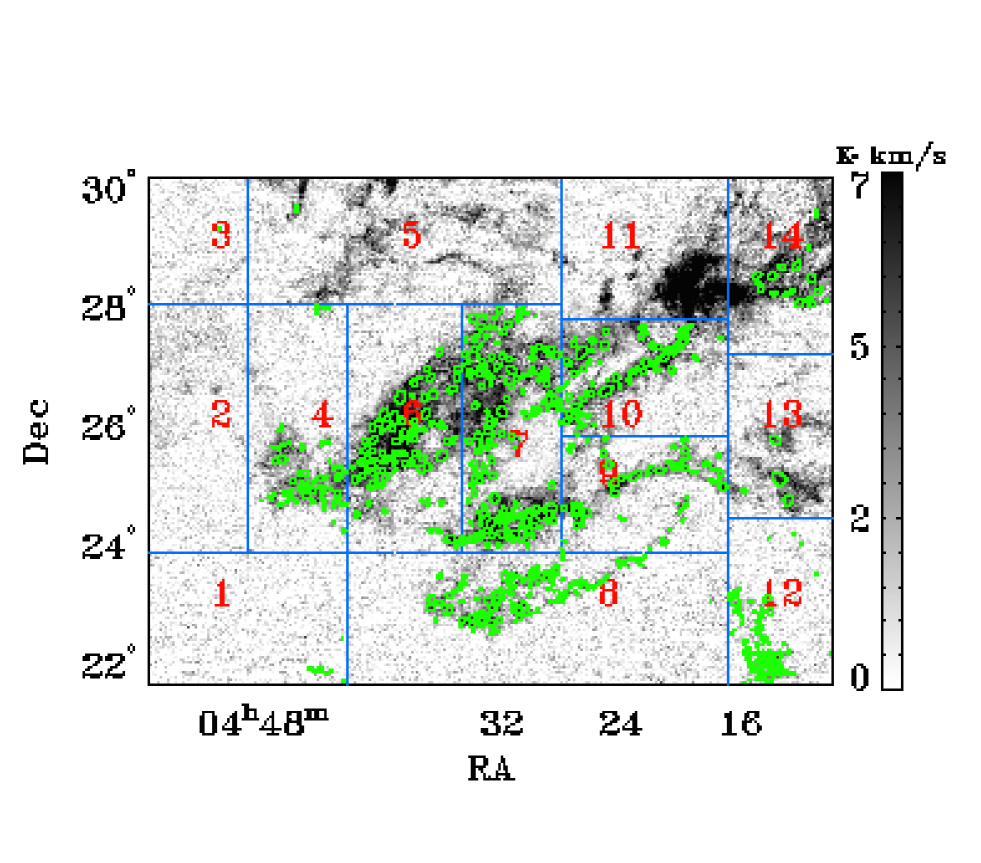
Figure 2: Image showing the total intensity of the ¹³CO emission in Taurus region. The data are divided into 18 regions for ¹³CO core fitting. The cores found by fitting gaussians to the ¹³CO data cube $(x,y,v)$ using GAUSSCLUMPS are shown as green ellipsoids. Despite the strong ¹³CO emission, no ¹³CO cores are found in region 11, and only one ¹³CO core is found in region 5. This can be understood by looking at the channel maps (see discussion in section 3).

The FWHM line width $\Delta V_{\rm FWHM}$ is calculated from the velocity dispersion of each ¹³CO core, $\Delta v$, which is the standard deviation of the velocity value about centroid velocity, weighted by the corresponding pixel data value.

$${\Delta V_{\rm FWHM}}=2\sqrt{2\ln 2}\Delta v\>\>.$$ (18)

The virial mass is also estimated from $\Delta v$ (Bertoldi & McKee, 1992)

$$M_{\rm vir}=\frac{5\Delta v^{2}R}{G}\>\>.$$ (19)

This equation describes a balance between the self gravity and combined thermal and nonthermal motions of a ¹³CO core, neglecting external pressure and the magnetic field. A core is considered gravitationally bound when its mass exceeds $M_{\rm vir}$.

In dealing with the extinction map, the hydrogen column density is estimated from optical extinction (Güver & Özel, 2009)

$$\frac{N_{\rm H}}{\rm cm^{-2}}=2.2\times 10^{21}\left(\frac{A_{V}}{\rm mag}\right)\>\>.$$ (20)

We have applied GAUSSCLUMPS with the fitting parameters listed in table 1 to the Taurus region to extract cores. We have also applied CLUMPFIND with the fitting parameters listed in table 2. In both cases, a background was first subtracted with the FINDBACK procedure using the same parameters listed in the tables. The cores fitted by GAUSSCLUMPS are shown in Figure 2 and those by CLUMPFIND in Figure 3. There are many more smaller cores found by CLUMPFIND, especially in the relatively diffuse region. This is attributable to CLUMPFIND’s requirement to assign one pixel to one particular core without ’splitting’ a pixel in possible overlapping configurations. We rely on the cores found by GAUSSCLUMPS in the subsequent analysis, since CLUMPFIND cannot split overlapping cores properly. In a study of core extraction with CLUMPFIND, Pineda et al. (2009) suggest not to blindly use CLUMPFIND to derive mass functions in any ”crowded” situation.

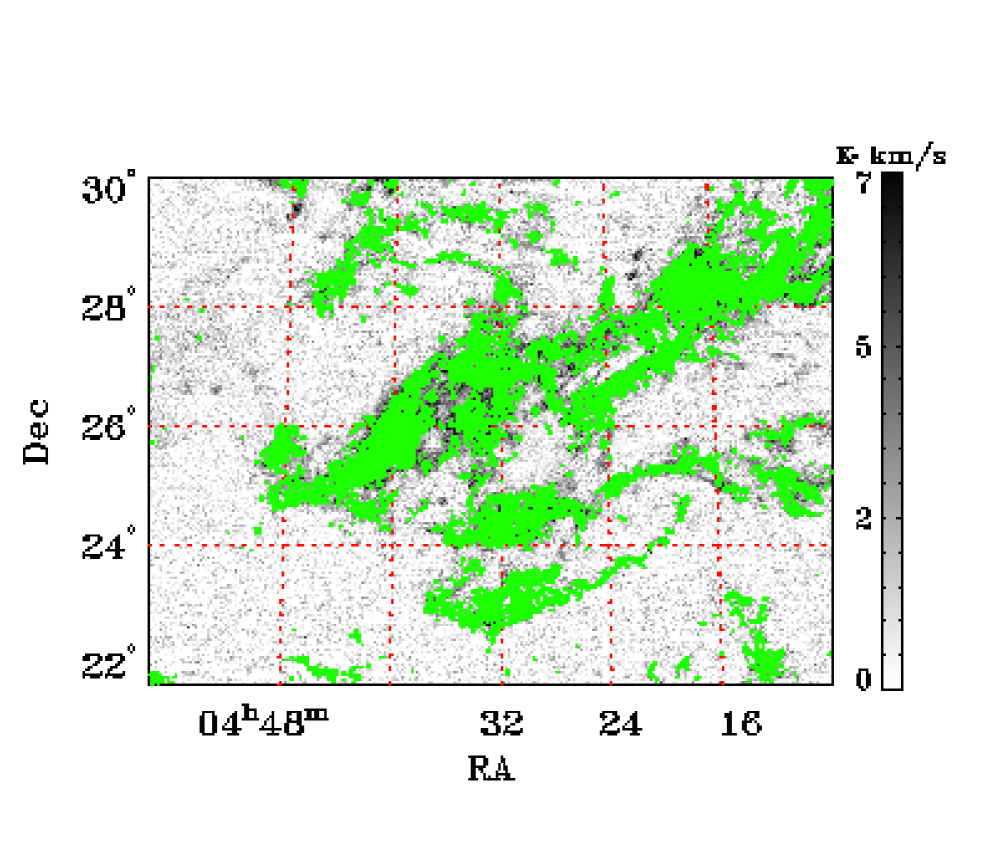
Figure 3: The cores found with CLUMPFIND routine are overlayed on the ¹³CO total intensity map. It is clear from this figure that the cores are ”crowded”. In this case, CLUMPFIND cannot extract cores properly.

Parameters of 3D ¹³CO cores and those cores found in the smoothed ¹³CO data cube can be found in tables LABEL:tab:clumps and LABEL:tab:clumps_smooth, respectively. In table LABEL:tab:clumpsEx, we give parameters of the cores derived from the 2MASS extinction map.

4 Results

We have performed a test on GAUSSCLUMPS by fitting to simulated data. We put 100 Gaussian components with random sizes and random locations into an empty simulation cube (an empty 3D array) with the size of region 1 in Figure 2. White noise (with $\sigma\sim 0.1$ K, a typical value across the Taurus region.) is also added to the whole cube as a background. This simulated data cube is then fitted by using the GAUSSCLUMPS tool. As a result, we find that for cores with peak intensity higher than 0.7K ($7\sigma$), the distribution of the cores found by GAUSSCLUMPS is similar to the simulated distribution. Figure 4 gives numerical results. For lower masses, GAUSSCLUMPS tends to find more cores (Stutzki & Guesten, 1990). Similar simulations have been done for the 2D data (¹³CO total intensity data and extinction data), where a threshold of $5\sigma$ is found to ensure agreement between measured and simulated distributions.

Figure 4: Core extraction from simulated data for ¹³CO by using GAUSSCLUMPS. The dashed line shows the distribution as a function of temperature of the simulated cores, while the solid line describes the cores extracted. When the core peak intensity is higher than $7\sigma\sim 0.7$ K, the difference is small. For peak intensity lower than $7\sigma$, GAUSSCLUMPS tends to extract more cores than are actually present. In this work only ¹³CO cores with peak intensity higher than 7$\sigma$ are included.

From the GAUSSCLUMPS fitting, we select cores with peak intensity higher than $7\sigma\sim 0.7$ K for ¹³CO data cube based on the simulation mentioned above, $5\sigma\sim 1.3$ K$\cdot$km/s for ¹³CO total intensity, and $5\sigma\sim 1.5$ mag for the extinction map, where $\sigma$ is the variance of data (the RMS). Other fitting parameters can be found in tables 1, 2, and 3.

Some filamentary structures (ellipses with a large axis ratio) were found in both the extinction map and the ¹³CO total intensity map. They comprise only a small fraction of the total mass (less than 10%). They do not show up in the fitting to the ¹³CO data cube, which means they are not ”coherent”, meaning that, the velocity variation within the structure cannot be described by a Gaussian in velocity space. Since the stability of a filament is different from that of a core (Lombardi & Bertin, 2001), we filter out those gaussian components that have an large axis ratio (major/minor $>$10) in the analysis. We thus obtain a sample of 765 ¹³CO cores. This is the largest sample of spectral line defined cores for a contiguous region (cf. Tatematsu et al., 1993; Aso et al., 2000; Ikeda et al., 2007; Tatematsu et al., 2008; Ikeda et al., 2009; Ikeda & Kitamura, 2009, 2011b).

Figure 2 shows the ¹³CO integrated intensity map overlayed with the cores obtained by Gaussian fitting to the ¹³CO data cube. Most of the regions with ¹³CO emission are found to contain cores. However, despite the strong ¹³CO emission in region 11 and 5, no ¹³CO core is found in the former and only one ¹³CO core is found in the latter. This is due to the rapid variation of intensity between velocity channels, which is clear in figures 5 and 6, which are the channel maps of region 11 and region 5, respectively. Gas in region 11 is likely to be affected by the young protostellar cluster within it (Schmalzl et al., 2010). In contrast to these two regions, the ¹³CO emission in all other regions containing ¹³CO cores is found to change gradually in velocity (see, e.g. figure 7).

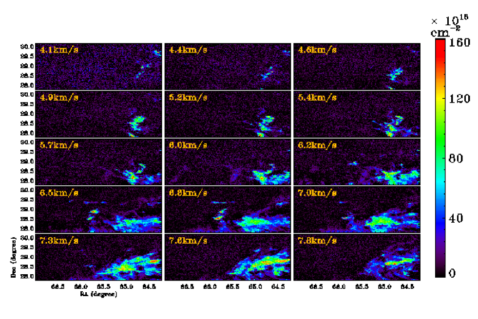
Figure 5: ¹³CO channel maps of the region 11 in figure 2. The intensity changes drastically between channels, which is in stark contrast with the region shown in figure 7 and suggests velocity incoherence in region 11. This is the reason why no ¹³CO core can be fitted by a three dimensional (x,y,v) gaussian in this region.

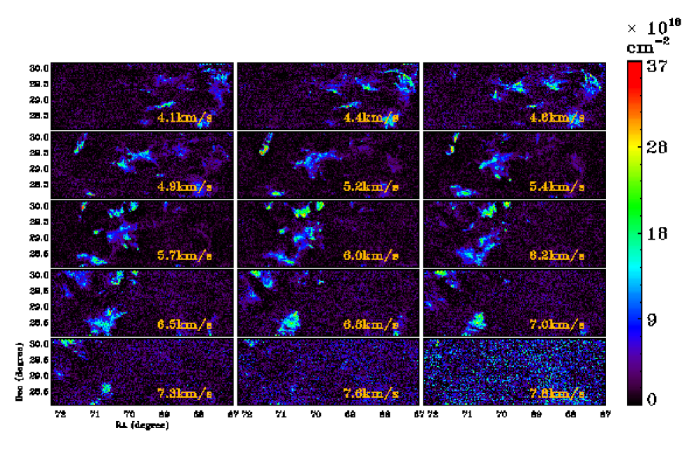
Figure 6: Channel maps of region 5 in figure 2. The intensity here also changes drastically between channels. Only one ¹³CO core is found in this region.

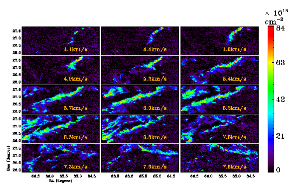
Figure 7: Channel maps of region 10 in figure 2. The main features are coherent through multiple channels and in consequence many ¹³CO cores are found in this region.

The distributions of the peak optical depth and the mean $\rm H_{2}$ density of the ¹³CO cores are shown in Figure 8. The mean $\rm H_{2}$ density is calculated by dividing the total number of $\rm H_{2}$ in a ¹³CO core by its volume, assuming its size along the line of sight is the same as its typical size (geometrical mean of major and minor, 2 times the typical radius in equation 3). Most of the ¹³CO cores have a typical $J=1\to 0$ optical depth of $\sim 0.8$ and a typical mean $\rm H_{2}$ density of $\sim 2000\ \rm cm^{-3}$. The recipes that we have adopted for optical depth correction and excitation state correction are adequate for cores in Taurus.

Figure 8: The distribution of the peak optical depth (left panel) and mean $\rm H_{2}$ density (right panel) of the ¹³CO cores.

By looking at the motion of the ¹³CO cores, we find a group of ¹³CO cores with systematically different line of sight velocities (see the lower corner of figure 16), which suggests these ¹³CO cores may not belong to the main cloud. After excluding these, we are left with 588 ¹³CO cores.

For comparison, we also use GAUSSCLUMPS to fit cores in the ¹³CO integrated intensity map with the procedures used for core fitting in the ¹³CO data cube. Figure 9 shows the ¹³CO integrated intensity map overlaid with cores obtained by Gaussian fit of the ¹³CO integrated intensity map, which is a 2D core fitting. Compared with the 3D core fitting to the ¹³CO data cube, there are cores found in the 2D core fitting within the regions having relatively abrupt, significant velocity variations seen in the ¹³CO data. This indicates that velocity is essential for reasonably defining cores in a complex cloud such as Taurus. The physical plausibility of requiring that a core have a relatively well-defined velocity in additional to a compact spatial structure eliminates many spurious cores that are identified in the 2D data alone.

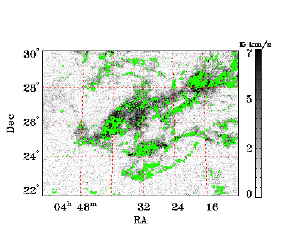
Figure 9: The cores found through a 2D Gaussian fitting of the ¹³CO total intensity map are overlaid on the ¹³CO total intensity map of the whole Taurus region. The red dashed lines are the coordinate lines of constant right ascension and declination.

Figure 10 shows dust extinction map overlayed with cores obtained by Gaussian fit to the 2MASS extinction map. The 200^′′ spatial resolution of 2MASS extinction map is about 5 times coarser than that of ¹³CO map. The extinction cores are generally larger than those found in ¹³CO data. We perform an experiment by smoothing the ¹³CO data to the same spatial resolution as 2MASS extinction and perform the core fitting. The fitted cores are also generally larger than those found in the original ¹³CO data, confirming that the cores found in the 2MASS data are generally unresolved even at the modest distance of Taurus (see table LABEL:tab:clumps_smooth).

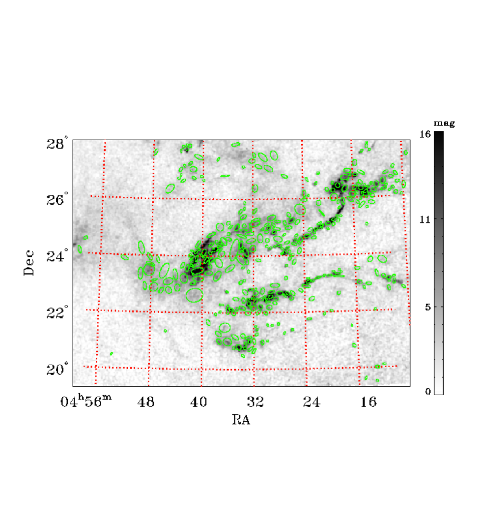
Figure 10: The cores found through a 2D Gaussian fitting of the extinction map are overlaid on the dust extinction map of the whole Taurus region. They are generally larger than the ¹³CO cores. The red dashed lines are the coordinate lines of constant right ascension and declination.

4.1 Mass distribution of the cores

We analyze the CMF in two functional forms, power law (equation 1) and log-normal (equation 2). Direct fitting of power laws to a cumulative mass function can be erroneous due to the natural curvature in the cumulative CMF (see the appendix in Li et al. (2007)). Therefore, we adopt a Monte Carlo approach similar to that used in  Li et al. (2007). We first generate a random sample of cores with one of the above distributions. For a power law distribution, there are three parameters, $M_{\rm max}$, $M_{\rm min}$, and $\gamma$, while for a log-normal distribution, there are two, $\sigma$ and $\mu$. The cumulative distribution $C(M_{i}),\ i=1,...,n$ of the random sample is then fitted to that of the sample found in the data $C_{0}(M_{i}),\ i=1,...,n$ by minimizing a $\chi^{2}$ function defined by

$$\chi^{2}\equiv\sum_{i=1}^{n}\frac{[C(M_{i})-C_{0}(M_{i})]^{2}}{C_{0}(M_{i})^{2}}\>\>.$$ (21)

The resulting mass function of the ¹³CO cores can be seen in figure 11. This mass distribution can be fitted much better by a log-normal function than by a power law, which only fits the higher mass end. The fitting results are similar for cores based on 2D fitting. The mass distribution that is based on 2D fitting of the ¹³CO integrated intensity can be fitted better with a lognormal function. The mass function of 2MASS extinction cores can also be fitted better with a log-normal function than with a power law (figure 12). Thus log-normal is a better representation of the mass distribution of cores than power law in the case of cores represented by ¹³CO, ¹³CO total intensity, and 2MASS extinction.

To examine the reliability and the completeness of the cores found, we calculate the minimum detectable mass for a core of certain size (Li et al., 2007)

$$M=M_{\rm point}\times\sqrt{N}\times\sqrt{M},$$ (22)

where $M_{\rm point}$ is the minimum detectable mass of a point source, and $N$ and $M$ are the number of pixels and number of velocity channels occupied by a core, respectively. We found this minimum detection mass is about 0.03 $M_{\odot}$ for a core as large as the smoothing scale. There is also another way to estimate the completeness (Pineda et al., 2009), with which similar result is obtained. All the cores found in the ¹³CO data cube are larger than this minimum mass. For the extinction map, the minimum detectable mass of a core is found to be about 0.8 $M_{\odot}$.

Figure 11: The mass distribution of the ¹³CO cores found by GAUSSCLUMP fitting to the ¹³CO data cube. The left panel shows the best fit power law distribution, while the right panel shows the best fit log-normal distribution, with the latter giving a better fit over the full mass range. The minimum detection mass for the ¹³CO cube is $0.03\ M_{\odot}$, indicated by the vertical dash-dotted line. We have fitted the mass function to ¹³CO cores more massive than the minimum detection mass. The fitting results are : (a) power-law distribution with $dN/d\log M\propto M^{-0.53}$, $M_{\rm max}=40.03\ M_{\odot}$, $M_{\rm min}=0.74\ M_{\odot}$. (b) log-normal distribution with $\mu=0.95$, $\sigma=1.15$.

Figure 12: The mass distribution of the cores found by GAUSSCLUMP fitting to the ¹³CO total intensity map (upper row) and to the extinction map (lower row). The panels on the left are fitted with power law distributions, while those on the right are fitted with log-normal distributions. The minimum detection masses are $0.03\ M_{\odot}$ and $0.8\ M_{\odot}$ for the ¹³CO data cube and the extinction map, respectively, and are indicated by vertical dash-dotted lines. The fitted results are: (a) $dN/d\log M\propto M^{-0.30}$, $M_{\rm max}=106.48\ M_{\odot}$, $M_{\rm min}=0.13\ M_{\odot}$. (b) log-normal distribution with $\mu=-0.62$, $\sigma=0.70$. (c) $dN/d\log M\propto M^{-0.1}$, $M_{\rm max}=92.0\ M_{\odot}$, $M_{\rm min}=1.2\ M_{\odot}$. (d) log-normal distribution with $\mu=2.04$, $\sigma=0.77$. The cores from ¹³CO total intensity and the extinction cores are both fitted better with a log-normal distribution than with a power law.

We used bootstrap (see e.g. Press et al., 1992) to estimate the uncertainty of the fitting. The resulting uncertainty is extremely small when the sample size is large. This means that the statistical uncertainty in our Monte-Carlo type fitting procedures is negligible. The difference between the fitted function and the data has to be systematic. For this reason, we do not show the numerical values of the uncertainties.

4.2 Energy State of ¹³CO Cores

We study the energy state of ¹³CO cores by analyzing the mass and line width together, which can only be accomplished through spectral maps. The properties of the 10 most massive ¹³CO cores are listed in table LABEL:tab:clumps for the ¹³CO data cube.

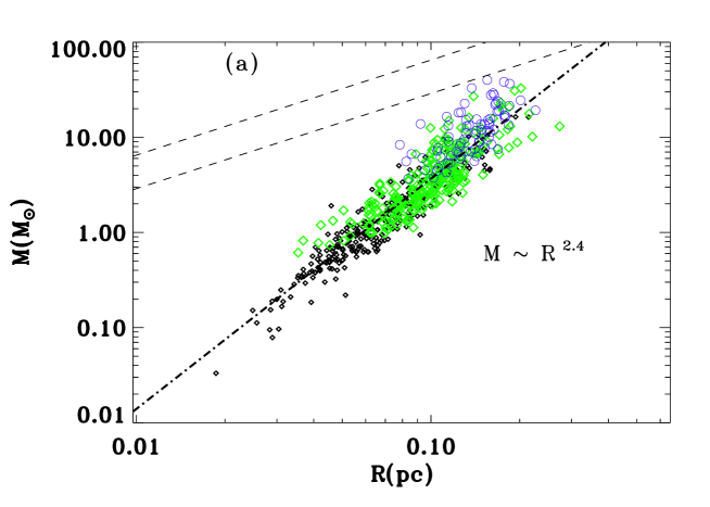
Figure 13: The mass-size relation of the ¹³CO cores found by GAUSSCLUMPS in the ¹³CO data cube. The Bonnor-Ebert mass is indicated by the dashed lines. The upper line corresponds to FWHM linewidth of 1.5 km/s and the lower line corresponds to 1.0 km/s.The mass-size relation is best fitted as $M\propto R^{2.6}$ indicated by the dash-dot line. ¹³CO cores with virial mass to mass ratio $M_{\rm vir}/M<2$ are denoted by blue circles; those with $2\leq M_{\rm vir}/M<5$ are denoted by green diamonds; other ¹³CO cores with $M_{\rm vir}/M>5$ are denoted by black diamonds.

Figure 14: The relation between the mass and size of the ¹³CO cores found in the extinction map (a) and in the ¹³CO total intensity map (b) with GAUSSCLUMPS. The mass-size relationship of extinction cores is best fitted with a power law $M\propto R^{2.0}$, while ¹³CO total intensity cores can be fitted with a power law $M\propto R^{2.4}$. The Bonnor-Ebert mass is indicated by the dashed lines. The upper line corresponds to FWHM linewidth of 1.5 km/s and the lower line corresponds to 1.0 km/s.

We investigate the mass-radius relation of the ¹³CO cores, which can be seen in figures 13 and  14. The core stability is studied by calculating the Bonnor-Ebert mass-radius relation (Li et al., 2007), in which the Bonnor-Ebert mass is obtained from integration of the density profile of the Bonnor-Ebert sphere

$$\rho(\xi)=\frac{1}{1+(\xi/2.25)^{2.5}}\>\>,$$ (23)

where the dimensionless radius $\xi$ is defined as

$$\xi=r\sqrt{4\pi G\rho_{c}/v_{s}^{2}}\>\>,$$ (24)

where $\rho_{c}$ is the central density and $v_{s}=\sqrt{kT_{\rm eq}/\mu m_{\rm H}}$ is the effective sound speed. The equivalent temperature $T_{\rm eq}$ is related to the FWHM line width $\Delta V_{\rm FWHM}$ with following equation  (Li et al., 2007),

$$T_{\rm eq}\equiv\frac{m_{\rm H}(3\Delta V_{\rm FWHM}^{2})}{8\ln(2)k}\>\>.$$ (25)

In our sample, the FWHM line width of the ¹³CO cores ranges from 0.5 km/s to 1.7 km/s. When $\xi$ is larger than $\xi_{\rm max}=6.5$, there is no longer any stable solution. With $\xi_{\rm max}$ and the size of a ¹³CO core, the central density $\rho_{c}$ is determined. The critical mass is then calculated by integration to the density profile (equation 23). Since the upper limit and the lower limit of the integration are constants, it is straightforward to show that the Bonnor-Ebert mass $M_{\rm BE}\propto r$.

A ¹³CO core having mass greater than its Bonnor-Ebert mass would be hydrostatically unstable. As can be seen in figure 12, no such ¹³CO cores (assuming a FWHM line width of 1 km/s) are found. This is in contrast to cores found in Orion, which are mostly supercritical (and thus unstable) (Li et al., 2007).

We have studied the mass distribution of nearly gravitationally bound ¹³CO cores (with virial mass to mass ratio $M_{\rm vir}/M<2$) and find that they can be well fitted with a log-normal function with $\mu=2.35$, $\sigma=0.52$ (see figure 15). The fact that a log-normal function fits the nearly gravitationally bound cores better than an Salpeter IMF type power law suggests that the mass conversion efficiency is NOT constant for all ¹³CO cores.

Figure 15: The mass distribution of those nearly gravitationally bound ¹³CO cores with virial mass to mass ratio $M_{\rm vir}/M<2$. The fitting results are (a) $dN/d\log M\propto M^{0.20}$, $M_{\rm max}=40.04\ M_{\odot}$, $M_{\rm min}=3.57\ M_{\odot}$. (b) log-normal distribution with $\mu=2.35$, $\sigma=0.52$. The log-normal distribution gives a good fit over the entire mass range that is sampled.

We also examine the virial mass of the ¹³CO cores according to Equation 19. Among the ¹³CO cores, there are 83 cores out of 588 that are nearly gravitationally bound (with the virial parameter $M_{\rm vir}/M<2$, see equation 19). The pressure from the surrounding materials also serves as confinement in addition to self-gravity, reducing the virial mass of a ¹³CO core (e.g. Kainulainen et al. (2011)). We can define an effective mass corresponding to the pressure by calculating the square of the effective velocity dispersion

$$\Delta V_{\rm eff}^{2}\equiv\frac{P_{\rm ext}}{\rho_{\rm core}}=\frac{kT_{\rm ext}}{m_{\rm H_{2}}}\frac{\rho_{\rm ext}}{\rho_{\rm core}}\>\>,$$ (26)

where $T_{\rm ext}$ is the temperature of the ambient medium. An effective mass is then defined analogously to the virial mass

$$M_{\rm eff}=\frac{f\Delta V_{\rm eff}^{2}R}{G}=\frac{fkT_{\rm ext}R}{m_{\rm H_{2}}G}\frac{\rho_{\rm ext}}{\rho_{\rm core}}=4.8\left(\frac{f}{5}\right)\left(\frac{R}{0.1\rm pc}\right)\left(\frac{T_{\rm ext}}{10\rm K}\right)\left(\frac{\rho_{\rm ext}}{\rho_{\rm core}}\right)M_{\odot}\>\>,$$ (27)

where $f$ is a dimensionless factor. For cores of the same mass, the pressure is a more important factor for the confinement of the less dense cores. The external pressure may be negligible for the confinement of a dense core, for example, considering a core with $\rho_{\rm ext}/\rho_{\rm core}\sim 1/100$, the effective mass would be about 0.05 $M_{\odot}$, which is negligible for a core having a total mass $\geq$ 1 M_⊙. The pressure is then unimportant for the confinement of massive cores, but is important for a core having total mass $\lesssim$ 0.1 M_⊙.

4.3 The Motion of Cores

Previous studies suggest that ¹³CO traces the bulk motion of dense gas as well as NH₃ and N₂H⁺ (Benson et al., 1998; Kirk et al., 2010). The cores are shown in figure 16 with the fitted centroid radial velocity coded in color. In general, the separation between the velocity of the core and that of the ambient gas is small. As seen in figure 17, the core centroid velocities are also mostly similar, except for cores in the lower right corner. This region differs systematically from the main Taurus cloud and may not be physically connected to it. After excluding these cores, there are 588 cores (out of 765 cores) left. We plot the velocity difference $\delta v$ vs. the apparent separation $L$ of these cores in figure 18.

Between the 588 cores there are $588\times(588-1)/2$ unique pairs, which are shown as the background density distribution in figure 18. The velocity difference $\delta v$ shows a bimodal distribution. We then calculate the dispersion of the velocity difference and plot the core velocity dispersion (CVD $\equiv\langle\delta v^{2}\rangle^{1/2}$). The relation between the CVD and the apparent separation between cores can be fitted with a power law, yielding CVD (km/s) $=0.2L({\rm pc})^{0.7}+0.2$ for $L$ between 0 and 10 pc, while those points having $L>10$ pc show large scatter, likely caused by under-sampling due to the finite size of the cloud. The mean value of the CVD for separation $L>10$ pc is $1.18$ km/s. The bimodal distribution in the velocity difference can be understood as defining two spatial scales. One corresponds to the typical size of a ”core cluster”, about 4 pc, while the other one shows the typical core cluster separation, about 8 pc.

To evaluate the significance of the bimodal distribution, we constructed a simple two-core-cluster model with 500 cores, with each cluster having a radius $R=7$ pc. The clusters are separated by 9 pc. A uniform spatial distribution of cores is assumed for both clusters. The velocity of a core is defined by a Gaussian with variance $\sigma$, given by $(\sigma/\sigma_{\rm max})=(D/R)^{0.5}$, where $D$ is the distance of the core from the center of the cluster it belongs to, and $\sigma_{\rm max}$ is the maximum $\sigma$ at the edge of a cluster, taken here to be 1.3 km/s. In practice, the line of sight velocity of a core is taken to be a random number from a gaussian distribution with variance $\sigma/\sqrt{3}$. There is an assumed systematic difference between the line of sight velocities of the two clusters, which is 1.8 km/s in our model. We are able to reproduce the major features of the observed CVD plot (figure 18) with this simple model. Rigorously speaking, the velocity of cores in each cluster do not follow the exact form of Larson’s law, because there is a center. However, the effect of such a distinction is negligible. We have tried to generate a sample of cores in which the velocity of a core is still gaussian distributed whose variance depends on its distance to the previously generated core, denoted as $l$, with the same relation $\sigma\propto l^{0.5}$, and get similar results to those shown in figure 18. The two length scales, i.e. the size of a core cluster, and the separation between the clusters are clearly seen in figure 19. The relation between the CVD and the apparent separation in the $L=0\sim 10$ pc region can be fitted by a power law of the form CVD (km/s) $=0.13L({\rm pc})^{0.7}+0.2$. In $L>10$ pc region, CVD can be fitted by a linear function of slope 0.04. The mean value of the core velocity difference in this region is $0.93$ km/s. We conclude that the main features of the observed CVD vs $L$ relationship and the observed $\delta v$ are reproduced reasonably well by this simple demonstration.

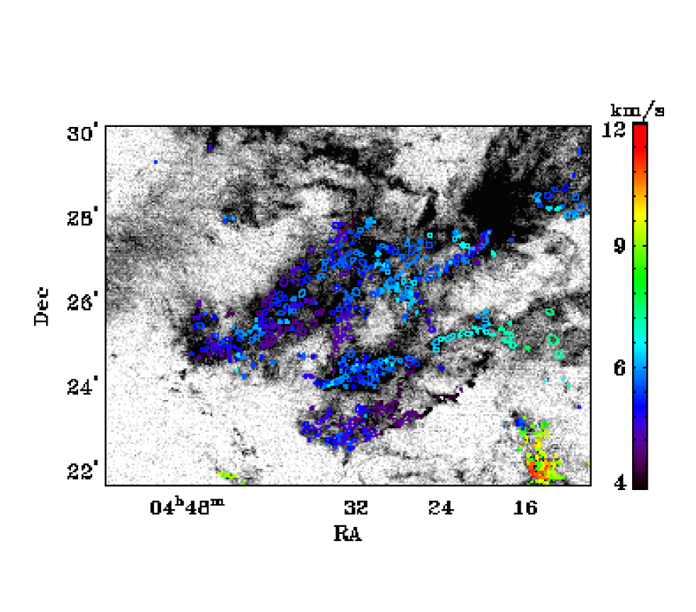
Figure 16: Overlay of the cores identified using the 3D ¹³CO data cube on the ¹²CO total intensity map with the centroid velocity coded as shown in the color bar on right. In most parts of Taurus, the core centroid velocities are similar. However, at the lower right corner, the centroid velocities of the cores differ systematically from those in other regions, which may suggest a different origin or location of these cores. In the study of the core velocity dispersion, we exclude these cores.

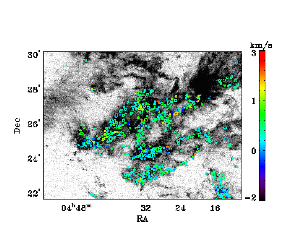
Figure 17: Overlay of the cores found in the 3D ¹³CO data cube on the ¹²CO total intensity map. The difference between centroid velocity of the cores and the local ¹²CO peak velocity is indicated by the color (coded in the color bar on right) and is generally small ($\leq$ 1 km/s).

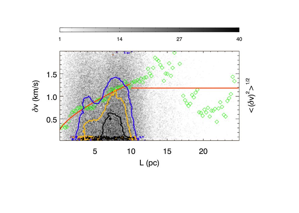
Figure 18: Plot of the core velocity difference, $\delta v$ vs. the apparent separation $L$ of cores and the core velocity dispersion (CVD$\equiv\langle\delta v^{2}\rangle^{1/2}$). The background is a image of the number of data points in the $\delta v-L$ plane, with grey scale (density bar at top of figure) showing the density of points. Contours of the density distribution in this plot are also shown. The green diamonds represent the variance of the velocity difference in each separation bin. The background density distribution shows two group of points, which are also evident by looking at the contours. These two groups define two length scales. One corresponds to the typical size of a ”core cluster”, about 4 pc, while the other one shows the ”core cluster” separation to be about 8 pc.

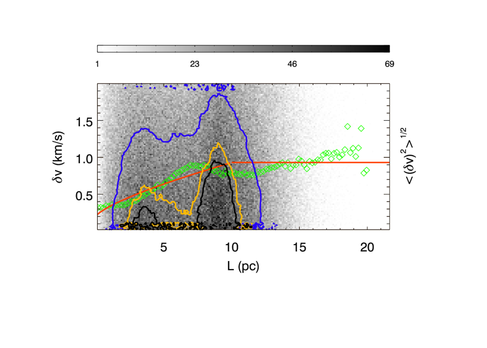
Figure 19: Results from numerically generated sample taken from two spherical clusters of cores, each having a 7 pc radius and with a separation of 9 pc between the centers of two clusters. The same statistical treatment as that applied to the actual data (figure 18) has been employed. The two length scales, i.e. the size of a core cluster, and the separation of the clusters are clearly seen. The points with apparent separation $0\geq L\leq 10$ pc can be fitted with a power law of CVD (km/s)$=0.13L({\rm pc})^{0.7}+0.2$. The horizontal line shows the mean $\delta v$ value, $0.93$ km/s, of points with $L>10$ pc.

5 Discussion

The shape of the core mass function has been for some time under scrutiny due to its possible relevance to the origin of stellar initial mass function. We found that a log-normal distribution best represents the ¹³CO CMF in Taurus, through fitting the 3D ¹³CO data cube.

We also searched for and studied the cores identified in the 2MASS extinction map. For extinction cores, a power law function is a better fit than a log-normal function. It is important to note the significant differences between 3D fitting and 2D fitting. In the former case, velocity information is invoked so that overlapping cores can be separated. We have compared the fitting to the 3D data cube and that to the 2D total intensity map (figure 20). There are some low-density cores that do not emerge in the fitting to the 3D data cube. There are overlapping cores, which can be separated in the 3D fitting by using the velocity information (an example of the spectrum is shown in figure 21). This is a direct demonstration of the peril of solely relying on total column density maps (such as dust continuum) to obtain core properties. In the light of these considerations, we believe that the CMF derived from extinction maps needs to be treated with some caution for interpreting the origin of the IMF, even though it may have a similar power-law form as that of the IMF.

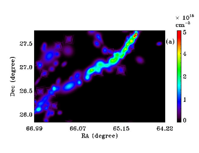
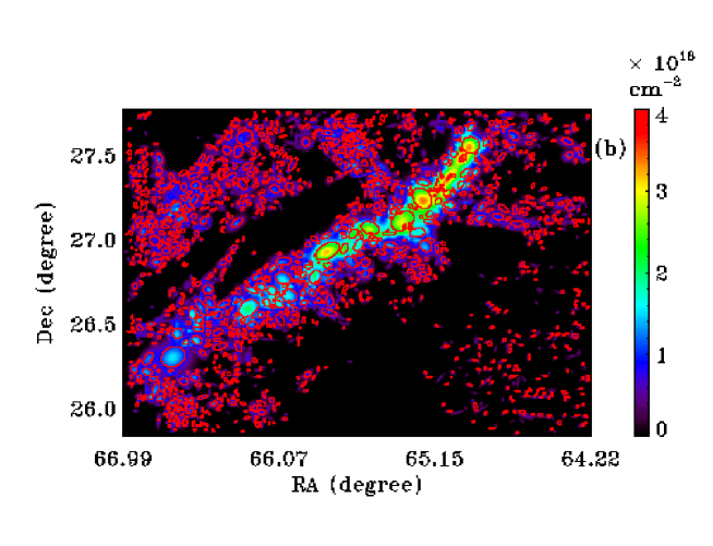
Figure 20: Fitting to a patch within region 10. The spectrum at the location of the red circle in the upper right of panel (a) is shown in figure 21. (a) The total intensity map of ¹³CO cores found in the data cube of region 10 (3D).(b) ¹³CO cores found in the total intensity of the original data of region 10 (2D). More cores are found in the 2D fitting, especially in the relatively diffuse regions. These cores contain large internal velocity variations.

Figure 21: An example spectrum containing contributions from two ¹³CO cores, which are clearly separated in velocity. The location where this spectrum was observed is indicated by the red circle in panel (a) of figure 20.

The large sample size and substantial spatial dynamic range of the Taurus ¹³CO core sample allow us to reconstruct the core velocity dispersion (CVD) for the first time. The CVD exhibits a power-law behavior as a function of the apparent separation $L$ between cores for $L<$ 10 pc (see figure 18). This is similar to Larson’s law for the velocity dispersion of the gas. The peak velocities of ¹³CO cores do not deviate from the centroid velocities of ambient ¹²CO by more than half the ¹²CO line width. The small velocity differences between dense and diffuse gas have also been noted by  Kirk et al. (2007) for Perseus cores. Simulation of core formation under the influence of converging flows suggest that massive cores exhibit relatively small line widths compared to less massive ones (Gong & Ostriker, 2011). We do not see this trend in our work, i.e. there is no apparent correlation between the mass and the line width or between the mass and the temperature (see figures 22 and 23). Padoan et al. (2001) found smaller line width in denser gas, which is not seen in Taurus sample either. These results suggest that dense cores condense out of the more diffuse gas without additional energy input from sources, such as protostars or converging flows.

Figure 22: The mass-line width relation of the cores found by GAUSSCLUMPS. There is no apparent correlation between the mass and the line width.

Figure 23: The mass-temperature relation of the cores found by GAUSSCLUMPS. There is no apparent correlation between these two quantities.

In recent simulations of core formation (e.g.  Gong & Ostriker, 2011) or star cluster formation (e.g. Offner et al., 2009), there is sufficient information to produce a CVD plot of the simulated core samples. Since CVD is sensitive to the dynamic history of core formation, we encourage the simulators to perform such analysis to facilitate direct comparison between theoretical models and observations.

6 Conclusions

We have studied the ¹³CO cores identified within the Taurus molecular cloud using a 100 $\rm degree^{2}$ ¹³CO $J=1\to 0$ map of this region. The spatial resolution of 0.014 pc and the velocity resolution of 0.266 km/s facilitate a detailed study of the physical conditions of ¹³CO cores in Taurus. The spatial dynamic range (the ratio of linear map size to the Nyquist sampling interval) of 1000 of our data set allows examination of the collective motions of ¹³CO cores and their relationship to their surroundings. We have found that the velocity information helps to exclude cores which we consider to be spurious.

Our conclusions regarding the extraction of ¹³CO cores and their properties are:

1) Velocity information is essential in resolving overlapping cores, allowing better resolution of cores and a more accurate determination of the CMF.

2) The mass function of the 3D(x,y,v) ¹³CO cores can be fitted better with a log-normal function ($\mu=0.95$ and $\sigma=1.15$) than with a power law function. For cores represented by ¹³CO total intensity and extinction, a log-normal distribution is also a better representation of the mass distribution than is a power law. There is no simple relation between the Taurus ¹³CO CMF and the stellar IMF.

3) No ¹³CO cores are found to have mass greater than the critical Bonnor-Ebert mass, in contrast to cores in Orion.

4) Only 10% of ¹³CO cores are approximately bound by their own gravity (with the virial parameter $M_{\rm vir}/M<2$). These can be well fitted with a log-normal mass function. External pressure plausibly plays a significant role in confining the ¹³CO cores with small density contrast to the surrounding medium.

5) In Taurus, the relation between core velocity dispersion (CVD$\equiv\langle\delta v^{2}\rangle^{1/2}$) and the apparent separation between cores $L$ can be fitted with a power law of the form CVD (km/s) $=0.2L({\rm pc})^{0.7}+0.2$ in the $0\leq L\leq 10$ pc region, similar to the Larson’s law, with a median value of 0.78 km/s.

6) The observed CVD is reproduced by using a simple two-core-cluster model, in which there are two core clusters with radius 7 pc and a separation 9 pc between these two clusters.

7) The low velocity dispersion among cores, the close similarity between CVD and Larson’s law, and the small difference between core centroid velocities and the ambient diffuse gas all suggest that dense cores condense out of the diffuse gas without additional energy input and are consistent with an ISM evolution picture without significant feedback from star formation or significant impact from converging flows.

8) The CVD can be an important diagnostic of the core dynamics and the cloud evolution. We encourage simulators to provide comparable information based on their calculations.

Table 1: Parameters used in the GAUSSCLUMPS fitting of the ¹³CO data cube and ¹³CO total intensity map.

Parameter	Value
WWIDTH	2
WMIN	0.01
MAXSKIP	100
THRESH	5
NPAD	100
MAXBAD	0.05
VELORES	2
MODELLIM	0.05
MINPIX	16
FWHMBEAM	2
MAXCLUMPS	2147483647
MAXNF	200

WWIDTH is the ratio of the width of the weighting function (which is a Gaussian function) to the width of the initial guessed Gaussian function.

WMIN specifies the minimum weight. Pixels with weight smaller than this value are not included in the fitting process.

MAXSKIP: If more than ”MAXSKIP” consecutive cores cannot be fitted, the iterative fitting process is terminated.

THRESH gives the minimum peak amplitude of cores to be fitted by the GAUSSCLUMPS algorithm. The supplied value is multipled by the RMS noise level before being used.

NPAD: The algorithm will terminate when ”NPAD” consecutive cores have been fitted all of which have peak values less than the threshold value specified by the ”THRESH” parameter. (From the source code cupidGaussClumps.c, one can see that the algorithm will do the same thing when ”NPAD” consecutive cores have pixels fewer than ”MINPIX”.)

MAXBAD: The maximum fraction of bad pixels which may be included in a core. Cores will be excluded if they contain more bad pixels than this value.

VELORES: The velocity resolution of the instrument, in channels.

MODELLIM: Model values below ModelLim times the RMS noise are treated as zero.

MINPIX: The lowest number of pixel which a core can contain.

FWHMBEAM: The FWHM of the instrument beam, in pixels.

MAXCLUMPS: The upper limit of the cores to be fitted. Set to a large number so this parameter do not take effect.

MAXNF: The maximum number of evaluations of the objective function allowed when fitting an individual core. Here it is just set to a very large number to guarantee all the cores to be fitted.

Table 2: Parameters used in the CLUMPFIND fitting of the ¹³CO data cube).

Parameter	Value
DELTAT	5.0*RMS
FWHMBEAM	2.0
MAXBAD	0.05
MINPIX	16
NAXIS	3
TLOW	5*RMS
VELORES	2.0

Table 3: Parameters used in the GAUSSCLUMPS fitting of the extinction map.

Parameter	Value
WWIDTH	2
WMIN	0.01
MAXSKIP	50
THRESH	5
NPAD	50
MAXBAD	0.05
VELORES	2
MODELLIM	0.05
MINPIX	16
FWHMBEAM	2
MAXCLUMPS	2147483647
MAXNF	200

Table 4: Properties of the cores found in 3D ¹³CO data cube.

ID	RA(∘)	DEC(∘)	$\mathbf{R}_{\rm major}(^{\prime})$	$\mathbf{R}_{\rm minor}(^{\prime})$	$\mathbf{\theta}$(∘)	T(K)	$\mathbf{M}$($\mathbf{M}_{\odot}$)	$\mathbf{M}_{\rm vir}$($\mathbf{M}_{\odot}$)	FWHM(km/s)	$\mathbf{n}_{\rm H_{2},mean}$(cm-3)
1	4h35m 38.5s	24d 6m 50.1s	4.5	3.2	55.9	12.9	40	32	1.0	3300
2	4h31m 49.7s	24d33m 2.1s	4.9	3.8	138.9	9.2	38	46	1.1	3820
3	4h23m 33.3s	25d 3m 22.6s	5.8	3.5	128.3	9.4	37	26	0.8	2480
4	4h26m 50.1s	26d13m 53.8s	4.4	2.6	95.3	7.9	33	14	0.7	3130
5	4h31m 52.1s	26d14m 42.7s	5.0	4.9	18.3	9.2	33	80	1.4	2470
6	4h28m 59.7s	24d30m 16.2s	5.0	4.5	106.7	9.4	31	93	1.5	5950
7	4h21m 4.2s	27d 4m 15.2s	4.5	3.5	94.1	9.4	29	47	1.2	4290
8	4h11m 15.5s	28d31m 31.7s	5.3	3.0	97.4	10.1	28	23	0.8	4330
9	4h39m 42.7s	25d45m 25.7s	4.2	3.7	103.6	10.6	28	47	1.2	3680
10	4h39m 10.9s	25d53m 45.0s	3.5	3.3	3.2	8.3	27	55	1.4	1780

Properties of the 10 most massive ¹³CO cores. Following the identifiers in column 1, the next two columns are the RA and Dec of the center of the fitted ¹³CO cores. The semi-major axis $R_{\rm major}$ and semi-minor axis $R_{\rm minor}$ of the fitted ¹³CO cores follow. The sixth column is the position angle of ¹³CO cores (angle from north to the major axis). The next column is the peak temperature of the ¹³CO cores. The mass $M$ and the virial mass $M_{vir}$ follow. Column 10 gives the full width to half maximum line width of the ¹³CO line. The last column shows the estimated mean $\rm H_{2}$ density of the ¹³CO cores.

Table 5: Properties of the cores found in the smoothed ¹³CO data cube.

ID	RA(∘)	DEC(∘)	$\mathbf{R}_{\rm major}(^{\prime})$	$\mathbf{R}_{\rm minor}(^{\prime})$	$\mathbf{\theta}$(∘)	T(K)	$\mathbf{M}$($\mathbf{M}_{\odot}$)	$\mathbf{M}_{\rm vir}$($\mathbf{M}_{\odot}$)	FWHM(km/s)
1	4h19m 31.2s	27d 8m 60.0s	6.8	4.4	153.9	8.0	104	154	4.3
2	4h21m 12.0s	27d 2m 24.0s	10.2	7.2	124.5	9.4	77	356	5.2
3	4h32m 43.2s	24d21m 36.0s	7.3	5.0	146.9	11.1	77	89	3.1
4	4h30m 52.8s	26d53m 24.0s	6.9	6.2	88.8	8.4	72	61	2.4
5	4h11m 14.4s	28d33m 36.0s	9.2	5.9	117.7	11.6	63	56	2.2
6	4h23m 38.4s	25d 0m 0.0s	7.9	5.6	133.7	10.3	47	48	2.2
7	4h31m 52.8s	26d17m 60.0s	6.0	5.2	6.5	10.0	35	94	3.3
8	4h32m 43.2s	26d 2m 60.0s	6.0	5.1	132.8	9.1	34	236	5.3
9	4h31m 43.2s	24d31m 48.0s	5.7	5.6	152.5	11.4	34	265	5.5
10	4h35m 45.6s	22d56m 24.0s	5.3	4.0	71.3	6.8	31	48	2.6

The columns are arranged as those of table LABEL:tab:clumps.

References

- Adams & Fatuzzo (1996) Adams, F., & Fatuzzo, M. 1996, ApJ, 464, 256
- Alves et al. (2007) Alves, J., Lombardi, M., & Lada, C. 2007, A&A, 462, L17
- Aso et al. (2000) Aso, Y., Tatematsu, K., Sekimoto, Y., et al. 2000, ApJS, 131, 465
- Benson et al. (1998) Benson, P., Caselli, P., & Myers, P. 1998, ApJ, 506, 743
- Bertoldi & McKee (1992) Bertoldi, F., & McKee, C. 1992, ApJ, 395, 140
- Blitz & Williams (1997) Blitz, L., & Williams, J. 1997, ApJ, 488, L145+
- Chabrier (2003) Chabrier, G. 2003, ApJ, 586, L133
- Curtis & Richer (2010) Curtis, E., & Richer, J. 2010, MNRAS, 402, 603
- Enoch et al. (2008) Enoch, M., Evans, II, N., Sargent, A., et al. 2008, ApJ, 684, 1240
- Frerking et al. (1982) Frerking, M., Langer, W., & Wilson, R. 1982, ApJ, 262, 590
- Goldsmith et al. (2008) Goldsmith, P., Heyer, M., Narayanan, G., et al. 2008, ApJ, 680, 428
- Gong & Ostriker (2011) Gong, H., & Ostriker, E. 2011, ApJ, 729, 120
- Güver & Özel (2009) Güver, T., & Özel, F. 2009, MNRAS, 400, 2050
- Hofner et al. (2002) Hofner, P., Delgado, H., Whitney, B., et al. 2002, ApJ, 579, L95
- Ikeda & Kitamura (2009) Ikeda, N., & Kitamura, Y. 2009, ApJ, 705, L95
- Ikeda & Kitamura (2011a) —. 2011a, ApJ, 732, 101
- Ikeda & Kitamura (2011b) —. 2011b, ApJ, 732, 101
- Ikeda et al. (2009) Ikeda, N., Kitamura, Y., & Sunada, K. 2009, ApJ, 691, 1560
- Ikeda et al. (2007) Ikeda, N., Sunada, K., & Kitamura, Y. 2007, ApJ, 665, 1194
- Johnstone & Bally (2006) Johnstone, D., & Bally, J. 2006, ApJ, 653, 383
- Johnstone et al. (2001) Johnstone, D., Fich, M., Mitchell, G., et al. 2001, ApJ, 559, 307
- Johnstone et al. (2000) Johnstone, D., Wilson, C., Moriarty-Schieven, G., et al. 2000, ApJ, 545, 327
- Kainulainen et al. (2011) Kainulainen, J., Beuther, H., Banerjee, R., et al. 2011, A&A, 530, A64
- Kirk et al. (2007) Kirk, H., Johnstone, D., & Tafalla, M. 2007, ApJ, 668, 1042
- Kirk et al. (2010) Kirk, H., Pineda, J., Johnstone, D., et al. 2010, ApJ, 723, 457
- Könyves et al. (2010) Könyves, V., André, P., Men’shchikov, A., et al. 2010, A&A, 518, L106
- Kramer et al. (1998) Kramer, C., Stutzki, J., Rohrig, R., et al. 1998, A&A, 329, 249
- Larson (1973) Larson, R. 1973, MNRAS, 161, 133
- Li (2002) Li, D. 2002, PhD thesis, Cornell University
- Li et al. (2007) Li, D., Velusamy, T., Goldsmith, P., et al. 2007, ApJ, 655, 351
- Lombardi & Bertin (2001) Lombardi, M., & Bertin, G. 2001, A&A, 375, 1091
- McKee & Ostriker (2007) McKee, C., & Ostriker, E. 2007, ARA&A, 45, 565
- Motte et al. (1998) Motte, F., Andre, P., & Neri, R. 1998, A&A, 336, 150
- Narayanan et al. (2008) Narayanan, G., Heyer, M., Brunt, C., et al. 2008, The Astrophysical Journal Supplement Series, 177, 341
- Offner et al. (2009) Offner, S., Hansen, C., & Krumholz, M. 2009, ApJ, 704, L124
- Padoan et al. (2001) Padoan, P., Juvela, M., Goodman, A., et al. 2001, ApJ, 553, 227
- Pineda et al. (2009) Pineda, J., Rosolowsky, E., & Goodman, A. 2009, ApJ, 699, L134
- Pineda et al. (2010) Pineda, J., Goldsmith, P., Chapman, N., et al. 2010, ApJ, 721, 686
- Press et al. (1992) Press, W., Teukolsky, S., Vetterling, W., et al. 1992, Numerical recipes in FORTRAN. The art of scientific computing
- Rathborne et al. (2009) Rathborne, J., Lada, C., Muench, A., et al. 2009, ApJ, 699, 742
- Reid & Wilson (2005) Reid, M., & Wilson, C. 2005, ApJ, 625, 891
- Reid & Wilson (2006a) —. 2006a, ApJ, 644, 990
- Reid & Wilson (2006b) —. 2006b, ApJ, 650, 970
- Salpeter (1955) Salpeter, E. 1955, ApJ, 121, 161
- Schmalzl et al. (2010) Schmalzl, M., Kainulainen, J., Quanz, S., et al. 2010, ApJ, 725, 1327
- Stahl & Wilson (1992) Stahl, O., & Wilson, T. 1992, A&A, 254, 327
- Stanke et al. (2006) Stanke, T., Smith, M., Gredel, R., et al. 2006, A&A, 447, 609
- Stutzki & Guesten (1990) Stutzki, J., & Guesten, R. 1990, ApJ, 356, 513
- Swift & Beaumont (2010) Swift, J., & Beaumont, C. 2010, PASP, 122, 224
- Tatematsu et al. (2008) Tatematsu, K., Kandori, R., Umemoto, T., et al. 2008, PASJ, 60, 407
- Tatematsu et al. (1993) Tatematsu, K., Umemoto, T., Kameya, O., et al. 1993, ApJ, 404, 643
- Tennyson (2005) Tennyson, J. 2005, Astronomical spectroscopy : An Introduction to the Atomic and Molecular Physics of Astronomical Spectra, ed. Tennyson, J.
- Testi & Sargent (1998) Testi, L., & Sargent, A. 1998, ApJ, 508, L91
- Torres et al. (2009) Torres, R., Loinard, L., Mioduszewski, A., et al. 2009, ApJ, 698, 242
- Wang et al. (2006) Wang, Y., Zhang, Q., Rathborne, J., et al. 2006, ApJ, 651, L125
- Whittet et al. (2007) Whittet, D., Shenoy, S., Bergin, E., et al. 2007, ApJ, 655, 332
- Williams et al. (1994) Williams, J., de Geus, E., & Blitz, L. 1994, ApJ, 428, 693
- Wilson et al. (2009) Wilson, T., Rohlfs, K., & Hüttemeister, S. 2009, Tools of Radio Astronomy
- Wilson & Rood (1994) Wilson, T., & Rood, R. 1994, ARA&A, 32, 191