The North American and Pelican Nebulae I. IRAC Observations

Abstract

We present a 9 deg² map of the North American and Pelican Nebulae regions obtained in all four IRAC channels with the Spitzer Space Telescope. The resulting photometry is merged with that at $JHK_{s}$ from 2MASS and a more spatially limited $BVI$ survey from previous ground-based work. We use a mixture of color- color diagrams to select a minimally contaminated set of more than 1600 objects that we claim are young stellar objects (YSOs) associated with the star forming region. Because our selection technique uses IR excess as a requirement, our sample is strongly biased against inclusion of Class III YSOs. The distribution of IRAC spectral slopes for our YSOs indicates that most of these objects are Class II, with a peak towards steeper spectral slopes but a substantial contribution from a tail of flat spectrum and Class I type objects. By studying the small fraction of the sample that is optically visible, we infer a typical age of a few Myr for the low mass population. The young stars are clustered, with about a third of them located in eight clusters that are located within or near the LDN 935 dark cloud. Half of the YSOs are located in regions with surface densities higher than 1000 YSOs / deg². The Class I objects are more clustered than the Class II stars.

1. Introduction

Much of our current knowledge regarding star-forming patterns and circumstellar disk evolution derives from study of molecular cloud complexes within a few hundred parsecs of the Sun. Among these are a large number of lower-mass clouds such as Taurus and, more infrequently, dense clouds like Orion, which is the prototypical high-mass and high density star forming region. While nearby cloud complexes serve as our primary empirical guide to understanding the formation and early evolution of stars, it is important that we study more than just the nearest examples. One little-studied-to-date star-forming region beyond the solar neighborhood is the North American and Pelican Nebulae (NGC 7000 and IC 5070, respectively), towards $l$=85, $b$=$-$0.5, about 600 pc from Earth. This region is probably more representative of star formation in the disk of the Milky Way than Taurus or Orion, it is also the next closest region after Orion with a substantial numbers of intermediate and high mass stars. The physical appearance of the nebulae on optical images is thought to reflect a combination of a large, background H II region (W80) overlaid by several foreground, dark clouds, with the edges of the dark clouds illuminated by the optically-unseen primary exciting star of the H II region. Because these nebulae lie essentially in the plane of the Galaxy and, as seen by us, along a spiral arm, study of the region is further confused by the juxtaposition of young stars and star-forming regions at a variety of distances. For the purposes of the rest of the paper, we will refer to the entire region as the NANeb, or the NAN complex.

Herbig (1958) was one of the first to study the star formation associated with these nebulae. He identified 68 H$\alpha$ emission line stars from objective-prism plates of the region, including a small cluster of pre-main sequence (PMS) stars in the “Gulf of Mexico” portion of the NANeb. Many of the young stars identified by Herbig lie along the bright rims of the dark clouds, possibly indicating that they are recent, second generation star formation products triggered by the expanding H II region from the first generation of stars in the NANeb. Herbig estimated a rough distance of 500 pc for the star-forming complex, but with a variety of caveats related to whether this distance applied to some or all of the stars and nebulae. The best available modern distance for the region appears to be that of Laugalys & Straižys (2002), who estimate a distance of $\simeq$600 pc. We will use this distance for the purposes of the paper with the caveats noted above.

Bally & Scoville (1980) mapped the CO associated with the dark clouds that define the Gulf of Mexico and Atlantic Ocean, and estimated that the mass in gas still present is of order $3\times 10^{4}\,M_{\odot}$. Their interpretation of the CO data was that the remaining dark clouds are the remnants of a much larger molecular cloud complex that has largely been disrupted by the hot, massive stars that were formed a few million years ago. Cambrésy et al. (2002) used the Two-Micron All-Sky Survey (2MASS; Skrutskie et al., 2006) point-source catalog to map the extinction and star clustering towards this region, deriving extinctions of $A_{v}\geq$ 35 magnitudes in some portions of the darkest cloud (Lynds 935). Cambrésy et al. also identified nine apparent star clusters in the 2MASS data.

Bally & Reipurth (2003) obtained narrow-band H$\alpha$ and [S II] imaging of the region of the Pelican nebula, and identified a number of new HH objects and collimated outflows, mostly originating from the interface region between the dark cloud and the H II region. In a couple of cases, the flows originate from near the tip of elephant trunks. The exciting sources for most of the flows could not be identified from the existing data. Armond et al. (2003) obtained additional narrow and broad band optical and near-IR imaging of the NANeb, and identified 28 more HH objects, including many associated with the PMS stars of Herbig’s Gulf of Mexico cluster. More recently, the probable exciting source for the H II region has been identified as an O5 star behind about $A_{V}$=10 mag of extinction, located inside the dark cloud LDN 935 separating the North America and the Pelican Nebulae (Comerón & Pasquali, 2005).

We have conducted a large ($\sim$9 deg²) infrared imaging survey with Spitzer Space Telescope (Werner et al., 2004) of this region, along with supporting data obtained in the optical for the $\sim 2.4\arcdeg\times 1.7\arcdeg$ central region. This present paper, the first of a series, presents the Infrared Array Camera (IRAC) data. Future papers will cover the Multiband Imaging Photometer for Spitzer (MIPS) data, with special emphasis on the Gulf of Mexico cluster (Rebull et al. 2009; hereafter R09), and the optical classification spectroscopy (Hillenbrand et al. in prep).

First, we present the observational details for the IRAC observations (§2). We then use the IRAC colors to select a minimally contaminated, if not complete, sample of YSO candidates (§3), and discuss their properties (classes, spatial distribution) in the context of other star-forming regions. Because IRAC is very sensitive to emission from HH objects, we then discuss the IRAC observations of one of the HH objects found in this region (§4).

2. Observations, Ancillary Data, and Basic Data Reduction

Table 1Summary of IRAC observations (programs 20015 and 462)

Program : field-ID	map center	AORKEY
P20015 : 12	20h55m30.00s,+44d59m00.0s	16790528
P20015 : 13	20h53m06.00s,+44d59m00.0s	16790784
P20015 : 21	20h57m54.00s,+44d23m00.0s	16791040
P20015 : 22	20h55m30.00s,+44d23m00.0s	16791296
P20015 : 23	20h53m06.00s,+44d23m00.0s	16791552
P20015 : 24	20h50m42.00s,+44d23m00.0s	16791808
P20015 : 31	20h57m54.00s,+43d47m00.0s	16792064
P20015 : 32	20h55m30.00s,+43d47m00.0s	16792320
P20015 : 33	20h53m06.00s,+43d47m00.0s	16792576
P20015 : 34	20h50m42.00s,+43d47m00.0s	16792832
P20015 : 42	20h55m30.00s,+43d11m00.0s	16793088
P20015 : 43	20h53m06.00s,+43d11m00.0s	16793344
P00462 : 0	20h50m38.00s,+45d05m10.0s	24251392
P00462 : 1	21h01m13.00s,+44d54m43.0s	24251648
P00462 : 2	20h58m51.00s,+45d12m42.0s	24251904
P00462 : 3	20h59m05.00s,+42d59m38.0s	24252160
P00462 : 4	21h00m17.00s,+43d23m25.0s	24252416
P00462 : 5	21h01m50.00s,+44d10m34.0s	24252672
P00462 : 6	20h50m19.00s,+42d58m37.0s	24252928
P00462 : 7	20h48m44.00s,+43d17m51.0s	24253184

2.1. Observations

The Spitzer observations of the NAN complex were obtained as part of the Cycle-2 program 20015 (PI: L. Rebull). Additional observations of the “corners” of the map were obtained as part of program 462 in an effort to increase the legacy value of the data set. The IRAC observations from program 20015 were obtained 9-11 August 2006, amd the IRAC observations from program 462 were obtained 15-27 November 2007. IRAC (Fazio et al., 2004) observes at 3.6, 4.5, 5.8, and 8 $\mu$m.

The Cycle-2 IRAC observations were designed to cover the region of highest extinction in a manner as independent of observing constraints as possible. Figure 1 is the NANeb region in the optical (from the Digitized Palomar Optical Sky Survey). The region covered by our IRAC map is indicated, as is the $A_{v}=5$ contour from the Cambrésy et al. (2002) extinction map. The observations were broken into 12 astronomical observation requests (AORs); the AORKEYs are given in Table 1. This region is at a high ecliptic latitude (+57^∘), so the field of view rotates by about a degree a day, necessitating small individual AOR coverage in order to completely tile the region without leaving gaps. Also, because of the high ecliptic latitude, asteroids are not a significant concern, and we therefore obtained all of the imaging at a single epoch. Each mapping AOR was constructed with the same strategy – at each map step, four dither positions were observed, each with high-dynamic-range (HDR) exposures of 0.6 and 12.0 second frame times. For this strategy, the on-line SENS-PET for a high-background region reports 3-$\sigma$ point-source sensitivities of 7.2, 10.7, 66, and 78 $\mu$Jy for the 4 IRAC bands, respectively. Differential source count histograms for our point sources are very similar to those for other star-forming regions observed in a similar manner - see in particular Figure 8 of Winston et al. 2007 (ApJ 669, 493) for 3.6 $\mu$m; the NaNeb histograms indicate that our 90% completeness limits are about [3.6] = 15 decreasing to about [8.0] = 12.5. For our purposes, however, the more important number is the completeness for detecting objects in all four channels. We estimate this by determining where the four-channel differential source counts drops below the 3.6 $\mu$m source counts by more than 20%, which occurs at about [3.6] = 12.2. This is about as expected given that four-channel catalog is normally limited by the detections in the 8.0 $\mu$m channel. This completeness limit corresponds to a spectral type of M4 or M1 according to the BCAH98 isochrones (Baraffe et al., 1998) for 1 or 5 Myr, respectively, a distance of 600 pc (assuming no reddening) and the temperature to spectral type scale defined by Luhman et al. (2003). The faintest object in our final catalog has [3.6]$\sim$16, corresponding to a mass of 0.02-0.03 M_⊙ at 1-5 Myr age, assuming the 3.6 $\mu$m flux is photospheric.

The remaining IRAC observations from program 462 were designed using the fixed-cluster observing mode to cover the irregularly-shaped regions to the same depth as the main map and to create a final map that is approximately square in shape. The map center given in Table 1 is the approximate center of each AOR. We used the software developed by R. Gutermuth and T. Megeath (private communication) for use by the IRAC GTO and Gould’s Belt teams to construct these AORs.

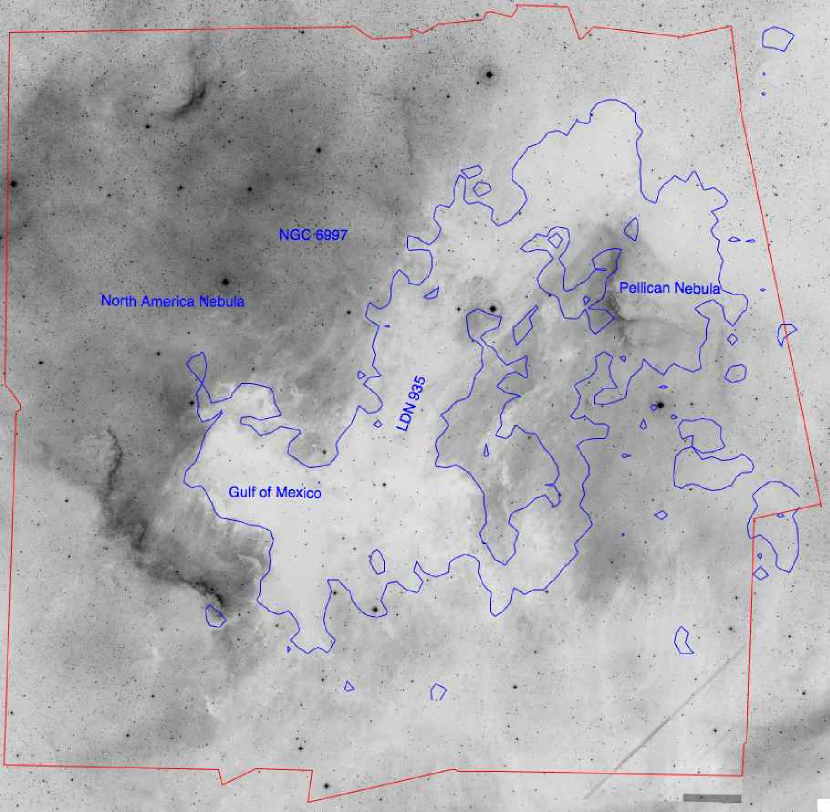
Figure 1.— Optical image ($\sim 4\times 3.2$ degrees) of the NANeb region from the Palomar all-sky survey. North is up, East is to the left. The left and right edges are at 21h02m32s and 20h46m52s; the top and bottom edges are at 45d25m40s and 42d40m56s. The region observed by IRAC is indicated by red lines. The green line is a smoothed $A_{v}$=5 contour from the Cambrésy et al. (2002) extinction map. The galactic coordinate of the center of this image is l=84.8, b=-0.6.

2.2. Basic Data Reduction

We started with the Spitzer Science Center (SSC) pipeline-produced basic calibrated data (BCDs), version S14.4. We ran the IRAC Artifact Mitigation code written by S. Carey and available on the SSC website. We constructed mosaics from the corrected BCDs using the SSC mosaicking and point-source extraction software package MOPEX (Makovoz & Marleau, 2005). The mosaics have a pixel scale of 1.22$\arcsec$ px^-1, very close to the native pixel scale. Figure 2 shows the mosaics in channel 1 (3.6 $\mu$m), and Figure 3 shows a 3-color IRAC mosaic (4.5, 5.8, and 8 $\mu$m).

We performed aperture photometry on the combined long- and short-exposure mosaics separately using the output of the APEX (par of the MOPEX software) detection algorithm (APEX is a part of the MOPEX package) and the “aper” IDL procedure from the IDLASTRO library. We used a 2 pixel radius aperture and a sky annulus of 2-6 pixels. The (multiplicative) aperture corrections we used follow the values given in the IRAC Data Handbook: 1.213, 1.234, 1.379, 1.584 for IRAC channels 1, 2, 3, and 4, respectively. Fluxes have been converted to magnitude given the zero magnitude fluxes of 280.9 $\pm$4.1, 179.7 $\pm$2.6, 115.0 $\pm$1.7 and 64.1 $\pm$0.9 for channels 1, 2, 3, and 4 respectively (IRAC Data Handbook). We take our photometry errors to be that given by the IDL procedure. We have checked that the uncertainties derived by the IDL procedure are consistent with the dispersion in IRAC colors for bright, off-cloud sources. For the longer integration times, the estimated average errors on our photometry in the 4 IRAC channels are 0.020, 0.025, 0.031, 0.035 magnitudes for bright stars, increasing to $\sim$0.1 mag for channels 1-4 at 15, 14.7, 13.2, 12.7 mag.

Since the sources have been extracted individually from the mosaiced BCDs, we have used the overlap between BCDs to estimate our astrometric precision. The histogram of coordinate differences shows a one sigma RMS uncertainty of 0.3$\arcsec$ ($\sim 1/4$ of pixel) in both directions.

The APEX source detection algorithm has a tendency to identify multiple sources within the PSF of a single bright source which can cause significant confusion at the bandmerging stage. Because our nominal fluxes are from the 2 pixel aperture photometry, any object which has a companion within 2 pixels will have a confused flux. The photometry lists were therefore cleaned of multiple sources prior to the bandmerging. Objects with a companion within 2 pixels had one of the sources removed. The source chosen for removal was the one with the lowest signal-to-noise ratio.

We extracted photometry from the long and short exposure mosaics separately for each channel, and merged these source lists together by position using a search radius of 2 pixels (2.44$\arcsec$) to obtain a catalog for each channel. The magnitude cutoff where we transition to using the long rather than the short exposure photometry corresponds to magnitudes of 11, 10, 8.4, and 7.5 magnitudes for channels 1, 2, 3 and 4 respectively.

Because of the complex nebulosity in this region, APEX (like any point-source detection algorithm) can be fooled by structure in the nebulosity. This effect is most apparent at 8 $\mu$m, where there are also the fewest stellar (point) sources detected. To attempt to remove false sources, we have compared photometry obtained via a 2 and 3-pixel aperture. After applying the aperture correction given in the IRAC Data Handbook, we eliminated sources with a difference of magnitude $>0.2$ mag; doing so rejected 32% of the raw detections in IRAC’s 8 $\mu$m band. This process is only applied to the 8 $\mu$m channel because the nebulosity is most prominent there (due to the presence of strong PAH bands at 7.6 and 8.6 $\mu$m). Also, because there are the fewest point sources detected in this band (see Table 2), the chances of there being two legitimate sources within 2-3 pixels of each other are much lower than in channels 1 or 2. Spot-checking the images confirms this assertion. We acknowledge this step may eliminate some true YSOs from our 4-band catalog. We deem this to be acceptable because our goal is to produce a minimally contaminated catalog of YSOs, not a complete catalog.

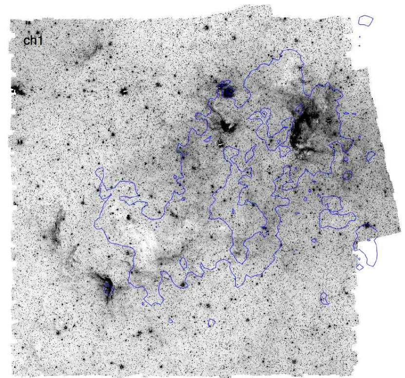
Figure 2.— Mosaic of the NANeb region from IRAC channel 1 (3.6 $\mu$m). Orientation and map center are the same as previous Figure; overlays from previous Figure are included for reference.

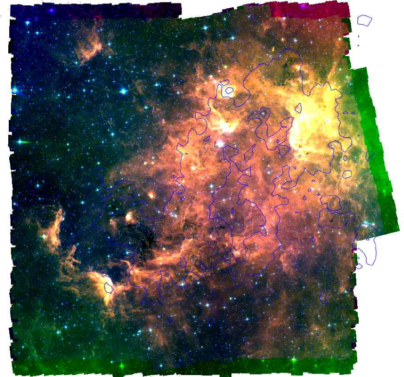
Figure 3.— A 3-color view of the IRAC NANeb with 4.5 $\mu$m in blue, 5.8 $\mu$m in green, and 8 $\mu$m in red. Orientation and map center are the same as Figure 1; overlays from Figure 1 are included for reference.

2.3. Ancillary Data & Bandmerging

Table 2 provides statistics for our entire catalog of objects; an object is included in our master catalog even if it is only detected in a single band. In order to create our final multi-wavelength catalog which we will use to identify new YSOs, we first merged the four individual IRAC source lists together, starting with IRAC-1, taking the closest source within 1$\arcsec$ as the best match. The radius of 1$\arcsec$ has been chosen based on our astrometric precision of 0.3$\arcsec$ (see section above) and the density of sources in the 3.6 $\mu$m image (i.e. the most crowded image).

In order to provide photometry at other bands, we cross-matched our catalog to 2MASS, taking the closest source within 1$\arcsec$, and then to our optical catalog, again taking the closest source within 1$\arcsec$. Out of the 63 084 objects detected at all 4 IRAC channels, 93% have a 2MASS counterpart. For the entire region, 10% of the final catalog stars have an optical counterpart; out of just the region covered by the optical photometry data, 28% have an optical counterpart. The MIPS catalog will be discussed in detail in R09. In summary, we have covered approximately the same area as the IRAC map, and we performed the source extraction using APEX.

$BVI$ images were obtained with the KPNO 0.9 m telescope on four photometric nights in June 1997. An area of approximately 2.4$\times$1.7 deg² was covered by mosaicing the $23.2^{\prime}\times 23.2^{\prime}$ FOV CCD in a grid with overlap of typically $3^{\prime}$ along each border. Exposures of 10 sec and 500 sec enabled unsaturated photometry between $V=11$ and 20 mag. In IRAF, images were bias subtracted and flat fielded with sky flats taken each night. Sources were identified using a 5$\sigma$ detection threshold and the DAOFIND task. The photometry was measured through an aperture of 5 pixels radius with background determined as the median in an annulus from 7-14 pixels where the plate scale was 0.68^′′/pixel. Aperture corrections were applied. Absolute photometric calibration was achieved through observation of Landolt standards and further self-calibrated across the overlap regions using stars in common between frames. First the short frames were calibrated to the long frames then the long frames were tied across the distinct telescope pointings, ignoring individual photometric errors larger than 0.1 mag. The average of the 43 spatial frame-to-frame offsets was 0.024 mag with dispersion 0.041 mag and a few frames requiring offsets as large as 0.1 mag. The individual offsets themselves have standard deviation typically 0.02-0.03 mag and standard deviation in the mean $<$0.01 mag, which we take as the self-calibration error. Photometry was adopted from the long frames except when in the nonlinear or saturated regimes of the CCD response in which case the short frame photometry was adopted; these criteria were applied at $B<$15.5, $V<$14.5, $I<$13.5. Astrometry was obtained using the HST Guide Star Catalog and the TASTROM task and is estimated accurate to $<$0.3” ($1\sigma$) based on stars in the overlap regions.

Additional $RI$ frames were obtained on a fifth night over a more limited area, $2\times 1.5\,$deg². These were reduced in a similar way, requiring a 5$\sigma$ detection threshold.

Table 2 Numbers of IRAC sources extracted from the NANeb data.

Band	Number of sources	Fractional number of sources which match (in %)
		$[3.6]$	$[4.5]$	$[5.8]$	$[8.0]$	$[3.6+4.5]$	$[3.6+4.5+5.8]$	$[3.6+4.5+5.8+8.0]$
$[3.6]$	558053	…	75	32	12	75	30	11
$[4.5]$	510922	82	…	33	13	82	33	12
$[5.8]$	200875	90	83	…	32	83	83	31
$[8.0]$	77898	84	83	82	…	83	81	81
$JHK_{s}$	220799	90	86	65	27	86	64	26
$BVI$	16595	85	83	72	40	83	71	39
$[24]$	4232	51	51	48	43	51	48	43

3. Identification and Characterization of our YSO Sample

3.1. Selection of YSO candidates

Several studies in the literature, usually focusing on subregions of this complex, have identified a total of $\sim$170 YSOs in the area covered by our IRAC map, using a variety of techniques such as NIR excess or H$\alpha$ emission. Most of these objects are earlier than K7. A complete list of the new Spitzer data for these previously-known YSOs will appear in R09.

Now, with our new, comprehensive multi-wavelength view of the complex, we can begin to create a census of the members of this complex having infrared excesses. However, doing so is difficult, as it requires an extensive weeding-out of the galactic and extragalactic contaminants. To begin this task, we have opted to create a minimally contaminated sample of Spitzer-selected YSO candidates, as opposed to identifying every possible YSO candidate. By miniminally contaminated sample, we simply mean a sample which includes as few non-YSOs as possible (i.e. from which AGB stars, AGN, and any other objects whose IR colors mimic YSOs have been eliminated). We identify only stars with excesses at IRAC wavelengths as YSOs – hence any member without excess (i.e. Class III YSOs) or stars with excess only at wavelengths greater than 8 $\mu$m (inner cleared regions or transitional disks) will not be included. We now discuss the selection criteria we have used to select our reliable YSO sample.

Our selection method is described below and illustrated in Figure 4. We initially require detection at all four IRAC bands, which substantially limits the catalog (see Table 2) and then we follow the IRAC four-band source characterization described in Gutermuth et al. (2008, section 4.1). Using their extragalactic contamination criteria, we have first rejected 272 sources as having colors consistent with galaxies dominated by PAH emission. This selection has been made in the $[4.5]-[5.8]/[5.8]-[8]$ and $[3.6]-[5.8]/[4.5]-[5.8]$ planes, where we reject objects seen in the grey zones plotted in panel (a) and (b) of Figure 4; this selection is defined by two sets of inclusive equations:

$$\begin{array}[]{c}\left\{\begin{array}[]{c}[4.5]-[5.8]<\frac{1.05}{1.2}([5.8]-[8.0]-1)\\ \&\\ \left[4.5\right]-[5.8]<1.05\\ \&\\ \left[5.8\right]-[8.0]>1\end{array}\right.\\ \\ \ \ \mathrm{OR}\\ \\ \left\{\begin{array}[]{c}[3.6]-[5.8]<\frac{1.5}{2}([4.5]-[8.0]-1)\\ \&\\ \left[3.6\right]-[5.8]<1.5\\ \&\\ \left[4.5\right]-[8.0]>1\end{array}\right.\end{array}$$ (1)

We then rejected 823 more sources having colors consistent with AGN in the [4.5] vs. [4.5]$-$[8.0] plane; the region of color space used to select AGN-like sources is plotted in panel (c) of Figure 4 and is defined by the following equations:

$$\begin{array}[]{c}\left\{\begin{array}[]{c}[4.5]-[8.0]>0.5\\ \&\\ \left[4.5\right]>13.5+([4.5]-[8.0]-2.3)/0.4\\ \&\\ \left[4.5\right]>13.5\end{array}\right.\\ \\ \ \ \&\\ \\ \left\{\begin{array}[]{c}[4.5]>14+([4.5]-[8.0]-0.5)\\ \mathrm{OR}\\ \left[4.5\right]>14.5-([4.5]-[8.0]-1.2)/0.3\\ \mathrm{OR}\\ \left[4.5\right]>14.5\end{array}\right.\end{array}$$ (2)

(see Appendix A of Gutermuth et al. 2008 for more details). Note that the AGN-like source selection has been made in the observed [4.5] vs. [4.5]$-$[8.0] plane, whereas Gutermuth et al. (2008) use the dereddened plane. Gutermuth et al. (2008) are able to work easily in the dereddened plane because they have a high spatial resolution $A_{v}$ map. Because the NAN complex is much further away than NGC 1333, we do not have the ability to construct such a high-resolution $A_{V}$ map. We tested the implications of this limitation by using the Cambrésy et al. (2002) extinction map to deredden individual objects. Just 25 sources would be dropped by performing this selection in the dereddened plane; they are fairly uniformly spread over the entire mapped region (and hence are likely contaminants rather than YSOs). Just 3 of these are in the Gulf of Mexico region (see R09) where we do not expect very much background contamination due to the very high reddening. Satisfied that this decision does not significantly affect our final sample of YSOs, we have chosen to keep our source selection in the observed plane.

Once these background contaminants are removed from consideration, we are left with a population of 61,989 IRAC sources, dominated by objects with the apparent colors of stellar photospheres. As in Gutermuth et al. (2008), we have further selected YSO candidates in the $[4.5]-[8]$ vs. $[3.6]-[5.8]$ color-color diagram meeting the following criteria:

$$\left\{\begin{array}[]{c}\left[4.5\right]-[8]>0.5\\ \&\\ \left[3.6\right]-[5.8]>0.35\\ \&\\ \left[3.6\right]-[5.8]\leq\frac{0.14}{0.04}\times\left([4.5]-[8]-0.5\right)+0.5\end{array}\right.$$ (3)

This selection is indicated in Figure 4, panel b. This leaves 1657 candidates.

Continuing to follow Gutermuth et al. (2008), we used their selection criteria to identify objects from the 1657 candidates whose IRAC fluxes may be contaminated by emission lines from shocks given their $[3.6]-[4.5]$ and $[4.5]-[5.8]$ colors by the equations:

$$\left\{\begin{array}[]{c}[3.6]-[4.5]>\frac{1.2}{0.55}([4.5]-[5.8]-0.3)+0.8\\ \&\\ \left[4.5\right]-[5.8]\leq 0.85\\ \&\\ \left[3.6\right]-[4.5]>1.05\end{array}\right.$$ (4)

We found only 2 YSO candidates that matched these criteria (205608.3+433654.2 and 205702.1+433431.3). Their SEDs are compatible with their being real YSOs whose aperture photometry is affected by emission from a compact, circumstellar nebula, causing an excess at 4.5 $\mu$m relative to the two adjoining IRAC bands. Moreover, these 2 objects are located inside the “Gulf of Mexico” where the concentration of YSOs is the highest in the cloud, and where previous optical emission line surveys have found numerous HH regions. Given these considerations, we retain these objects in our YSO candidate list.

Of the 1657 YSO candidates, 972 (59%) have a 2MASS counterpart. Out of the entire region, 131 (7.9%) have an optical counterpart; out of the region covered by the optical data, 10.4% have an optical counterpart. All but 63 of the YSO candidates are inside the region covered by MIPS data, and 45% of the candidates have a MIPS 24 $\mu$m counterpart. We note that the percentage of 2MASS and optical YSO counterparts is less than for the whole IRAC 4-band catalog (92% and 28% respectively, see section 2.3); this is due to the fact that YSOs are mostly located inside highly reddened regions and are not detected in our shorter wavelengths. With this selection of $\sim$1600 YSOs, we have increased the number of likely YSOs in the NANeb region by an order of magnitude.

We compare the positions of both the YSO candidates and background contaminants in a 2MASS / IRAC color color diagram in panel d of Figure 4. A large fraction (90%) of sources flagged as galaxies or AGN fall in the region occupied by reddened main sequence stars, and hence blueward in $K_{s}-[4.5]$ color from the YSOs. Just 5% of the YSO candidates are located in this same region, two-thirds of which are classified as intermediate between Class II and Class III (see §3.3).

It is hard to estimate the contamination fraction of our YSO candidates without additional data (e.g. spectroscopic or X-ray confirmation). However, we can make a few worst case estimates. Because our survey area is fairly large, it includes some sections which are outside the main star-forming region and have relatively few candidate YSOs. The north-east corner of our survey region (see Figure 3), for example, offers one such relatively YSO-poor area. Specifically, we define a “field” region as being the area above a line from the mid-point of the East edge of Figure 3 to the mid-point of the North edge of the figure. If all the candidate YSOs in this region are contaminants, we derive a contaminant surface density of 32 objects per square degree. Assuming the AGN and other contaminants are uniformly distributed over our survey region, this yields an upper limit to the fraction of contaminants in our survey of 17%.

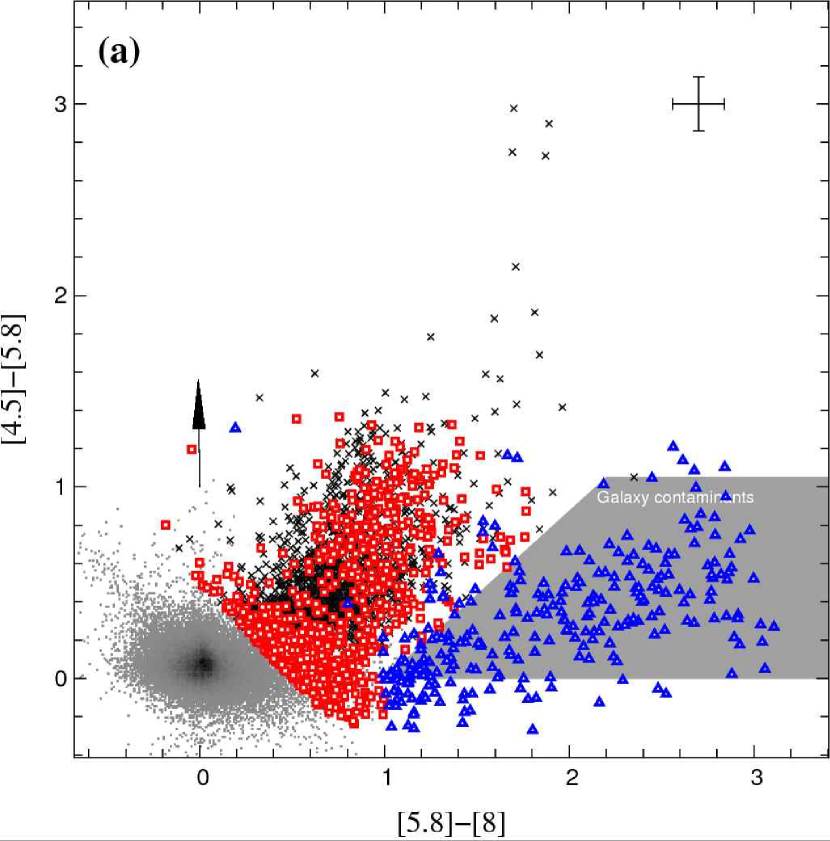
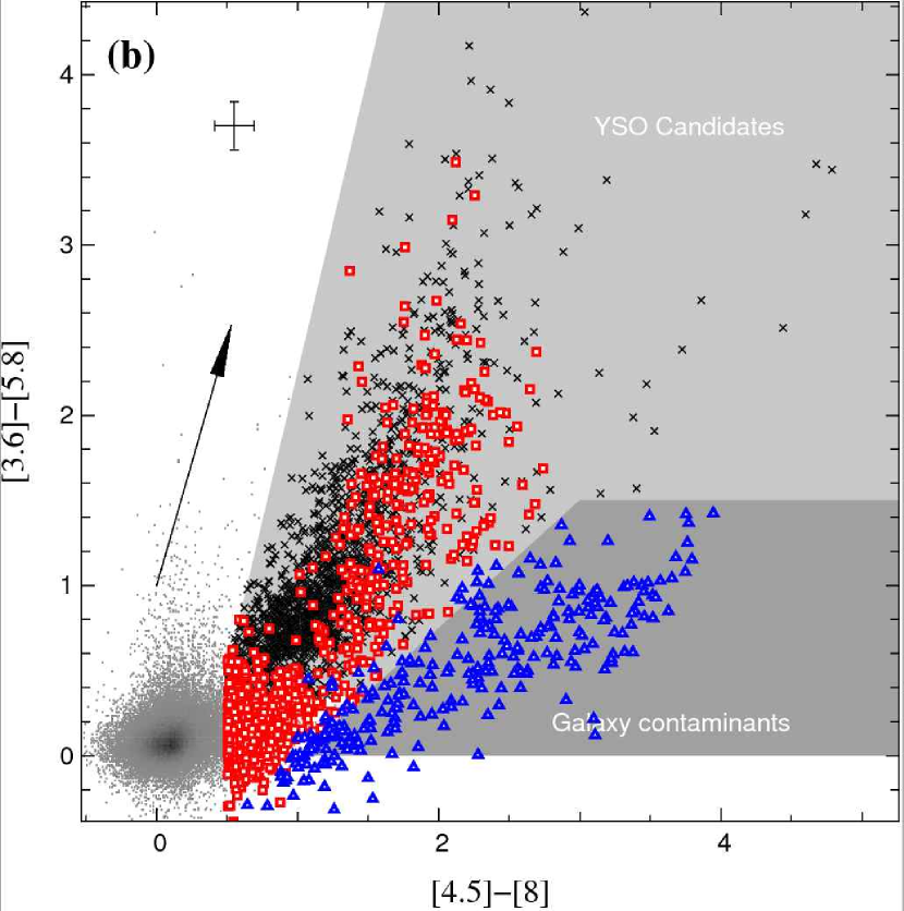
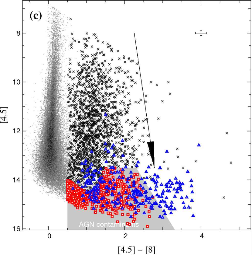
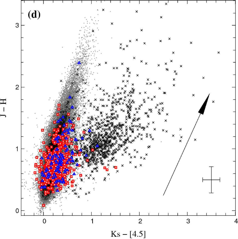
Figure 4.— IRAC color-color and color magnitude diagrams used to reject background contaminants (panel a, b and c) and select YSOs candidates (panel b). An additional diagram shows the distribution of background contaminants and YSO candidates in a 2MASS-IRAC color-color diagram limited to targets with 2MASS counterparts (panel d). In all diagrams, blue triangles are sources flagged as PAH-emission sources (galaxies) located in the darkest gray area of panel a or b. Red squares are sources flagged as AGN, selected in the gray area of panel c. Finally, YSOs candidates are plotted with black cross symbols; they have been selected in the brightest gray area of panel b if not previously flagged as background contaminants. The reddening vectors correspond to an $A_{K}$ of 10 in panels a, b and c, and $A_{K}$ of 2 in panel d. We averaged the extinction law given in Flaherty et al. (2007) for Serpens, Orion and Ophiuchus.

3.2. NANeb age estimation

We have used optical photometry in order to constrain the age of the NANeb complex. Figure 5 shows the location of YSOs with optical and 2MASS photometry in an optical color-magnitude diagram. Also shown are Siess et al. (2000) isochrones, where the color-$T_{\rm eff}$ conversion has been tuned so that the 100 Myr isochrone follows the single-star sequence in the Pleiades (Stauffer, 1996; Jeffries et al., 2007). The number of YSOs in this diagram is limited by the fact that it requires optical counterparts. This means that most of sources from this diagram are located inside the less-extincted regions of the NANeb, on the edge of the Pelican Nebulae (80% are located inside region of $A_{v}<5$, according to the Cambrésy et al., 2002 extinction map). The embedded Class I sources are not well-detected in the optical data, and our YSO selection criteria do not allow us to detect Class III sources, so this sample is mostly limited to Class II sources.

Figure 5.— $V/V-I$ color magnitude diagram for our YSO candidates. The solid lines are, from right to left, tuned Siess models (see text) for 1 3 and 10 Myr scaled to the NANeb distance. A reddening vector of $A_{v}$=5 is plotted.

Our age estimates are uncertain for all of the normally expected reasons (e.g. uncertainties in the isochrones and their transfer to the observational plane; the need for and imprecision of the reddening corrections; the effect of spots and UV excesses on the estimated colors and effective temperatures of our target stars; binarity). However, it is apparent in Figure 5 that most of our YSO candidates (with optical counterparts) are younger than 10 Myr according to the isochrone tracks. The median age is slightly older than 3 Myr, but the most embedded and probably youngest regions of NANeb are excluded from this optical CMD. The median age and the age dispersion is comparable to what found in NGC 2264 by Rebull et al. (2002). Since the reddening vector is essentially parallel to the isochrones, and YSOs with optical counterpart have low reddening, the median age will be minimally affected by reddening.

3.3. Classes of YSO Candidates

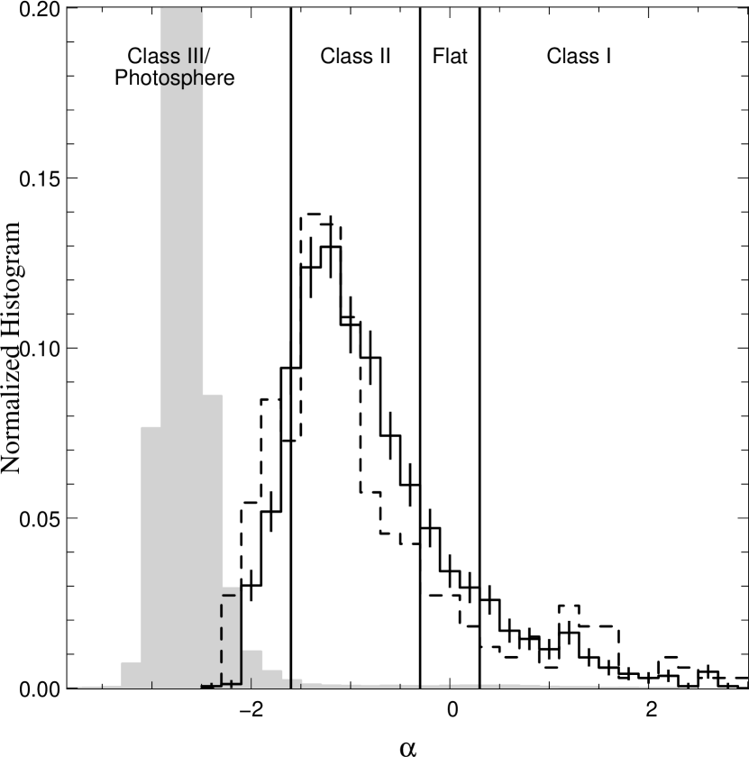
Figure 6.— Normalized histograms of the distribution of spectral slope, $\alpha$. The continuous line is the histogram for the YSO candidates for the whole sample. All other IRAC sources from the NANeb are also indicated (in gray), as are the 330 YSO candidates we have found from the Harvey et al. (2006) highly reliable catalog (dashed line).

We classified this set of highly likely NANeb YSOs, according to the Lada (1987) Class I/II/III system, updated by André (1994) where the “flat” class has been added between Class I and II. Classes are assigned based on the spectral index, defined by

$$\alpha=\frac{d\ \log{\lambda F(\lambda)}}{d\,\log{\lambda}}$$

where $F(\lambda)$ is the flux at the wavelength $\lambda$. For Class I, 0.3$\leq\alpha$; for flat sources, $-0.3\leq\alpha<0.3$; for Class II, $-1.6\leq\alpha<-0.3$; and for Class III, $\alpha<-1.6$. Note that because we are making a Spitzer-based selection of YSO candidates, by definition none of our candidates will have a photospheric slope, so our Class III inventory is guaranteed to be incomplete. Further observations at other wavelengths (e.g. with Chandra) are required to find such objects. In the following, to avoid confusion, we call our YSO candidates with $\alpha<-1.6$ Class II-III.

We fit $\alpha$ over the 4 IRAC channel points from 3.6 to 8 $\mu$m. From the total 1657 YSO candidates, we found that 1059 (64%) are Class II, 184 (11%) are flat and 198 (12%) are Class I. We classified the remaining 216 (13%) YSOs as Class II-III because they have $\alpha$ between stellar photospheres ($\alpha=-2.7$) and Class II ($\alpha=-1.6$). A histogram of $\alpha$ for our YSO candidate sample is plotted in Figure 6. This figure also contains, for comparison, a histogram of the values of $\alpha$ for our entire NANeb catalog (mostly field stars), and that for the YSO candidates derived from the highly reliable Serpens catalog obtained by Harvey et al. (2006, 2007b, 2007a) (see discussion below).

Plots similar to those appearing here (or in R09) can be found in most of the c2d series of papers on Serpens, Perseus, Ophiuchus, Chamaeleon II, and Lupus. We picked Serpens for our primary comparison here because it is thought to be similar in age to the NANeb, it contains a deeply embedded cluster similar to the Gulf of Mexico, it is in the Galactic plane ($l$=32, $b$=+5), and Harvey et al. (2006, 2007b, 2007a) performed a Spitzer-specific source selection. However, there are some important differences. The Spitzer maps of Serpens are only 0.85 deg², nearly 6 times smaller than our map. The selection method for finding YSO candidates is much different in Harvey et al. (2006, 2007b, 2007a), for example, requiring a MIPS-24 detection, and the differences are most strongly apparent in the selection of Class III objects.

In order to fairly compare our data with the Serpens data, we used the highly reliable Serpens catalog (of all objects, not just their YSO candidates) provided by the c2d team as part of their final Legacy delivery (available on the SSC website) and applied our selection method to those data. From the sample of Serpens YSOs which pass our selection criteria, we calculated $\alpha$ in the same way that we did for the NANeb, from 3.6 to 8 $\mu$m. It is these values which appear in Figure 6. Our selection and classification scheme yield 52 Class I, 24 Flat disk, 189 Class II and 65 Class II-III Serpens YSOs. The number of Class II-III objects is hard to compare to that found in Harvey et al. (2006) since they use the 24$\mu$m data in their classification scheme ; but the number of Class I, Flat and Class II are roughly comparable: 30, 33, 163 respectively in Harvey et al. (2006).

As a means to estimate a comparative evolutionary age for the NANeb stars, one can determine the ratio of the number of Class II (“older”) to Class I or Flat sources (“younger”), and compare that ratio to that derived for other clusters, such as Serpens. For our entire NANeb YSO sample, we derive a ratio N(Class II)/N(Class I+Flat) = 1059/382 = $2.78\pm 0.17$. Using our similarly analysed data for Serpens, we derive this ratio as $2.49\pm 0.33$ (roughly comparable to what was derived by Harvey et al. 2006 - $2.6\pm 0.4$, where they used 2MASS through 24 $\mu$m data to compute alpha). The ratios for NANeb and Serpens are comparable, suggesting that the mean ages of the two YSO samples are indeed similar.

Harvey et al. (2006, 2007b, 2007a) used a series of Spitzer-based selection criteria to select a sample of YSOs; their final selection in Harvey et al. (2007a) primarily uses color-color and color-magnitude diagrams to assign a liklihood that a given object is extragalactic. The process starts with requiring detection in all 4 IRAC bands as well as MIPS-24. Only about half of our minimally contaminated YSO sample has a MIPS-24 detection, so the Harvey et al. selection process by its very nature could only retrieve about half of our sample. However, $\sim$90% of our highly reliable sample with MIPS-24 detections is also retrieved by a Harvey et al.-style source selection.

R09 contains a special discussion of the Gulf of Mexico, which is an interesting area containing hundreds of deeply embedded young stars, mostly associated with 3 subclusters. We note here that our requirement for having all four bands of IRAC for our source selection omits many of the objects in this region, and this requirement will be relaxed in R09 to find cluster members. However, using our selection criteria and our best possible YSO sample (as defined above) results in a ratio of N(Class II)/N(Class I+Flat) that is statistically significantly different inside the Gulf cluster than outside of it. The ratio, with its Poissonian error, is 901/261=3.45 $\pm$0.24 outside the Gulf of Mexico and 158/121=1.31 $\pm$0.16 inside this region. Moreover, we find comparatively very few Class II-III objects in the Gulf of Mexico region. Both these findings indicate that the Gulf of Mexico cluster is, in evolutionary terms, the youngest region within the NAN complex.

We explore now, how the NANeb reddening can change our YSO classification. Indeed Muench et al. (2007), appendix A, demonstrated that for a deeply embedded cluster (A${}_{v}\sim$40), the IRAC SED slope of a typical K6 Class II member of IC 348 would be reddened into an apparent flat spectrum. According to the Cambrésy et al. (2002) extinction map, however, 97% of YSOs are located in region where the A_V is less than 10. Since the Cambrésy et al. (2002) map yields extinctions up to about 30, we assume that for extinctions $\leq$ 10 the predictions should be reliable (i.e. not “saturated” because the extinctions are so high that no background stars are present within the grid point). To test the effect of reddening on our classification, we have dereddened our SEDs prior to the spectral slope calculation, according to the Cambresy et al. map. The numbers of Class I, Flat disk and Class II given by the dereddened SEDs - 186, 177, 1043 - are quite similar to those using the observed SEDs - 198, 184 and 1059, making the N(Class II)/N(Class I+Flat) ratio equal to 2.87$\pm$0.17 instead of 2.78$\pm$0.17. This small differences does not change our main conclusions about the spatial distribution of Class I and Class II.

There is another means by which we can gauge the effect of extinction on our YSO classification. Gutermuth et al. (2008) distinguished protostars and Class II by there $[4.5]-[5.8]$ color excess. They chose this criterion specifically because it is relatively immune to extinction (because the interstellar extinction curve is relatively flat between these two wavelengths). Gutermuth et al. (2008) selected protostars as sources matching the following equation:

$$\left\{\begin{array}[]{c}\left[4.5\right]-[5.8]>1\\ \mathrm{OR}\\ \left[4.5\right]-[5.8]>0.7\&[3.6]-[4.5]>0.7\end{array}\right.$$ (5)

The Gutermuth et al. (2008) classification scheme does not include flat-spectrum sources as a separate class. Figure 7 shows the location of Class I / Flat / Class II and Class II-III YSOs in the $[4.5]-[8.0]/[3.6]-[4.5]$ plan superimposed on the protostar area defined above. The location of our Class I and Class II sources agree well with the regions defined in this diagram: 95% of our Class I and 99% of our Class II sources would be classified as protostars and Class II by the Gutermuth et al. criteria. Our flat spectrum sources lie on the border between Class I and Class II, with roughly equal numbers on either side of the Gutermuth et al. (2008) boundary.

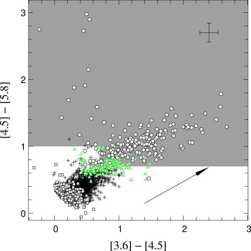
Figure 7.— Spitzer color-color diagram. Open squares are Class II-III, plus symbols are Class II, green triangles are classified as Flat spectrum sources and circles are Class I. The green area is the protostar selection area defined by Gutermuth et al. (2008). A reddening vector of A_k=10 is plotted.

3.4. Spatial Distribution of YSO Candidates

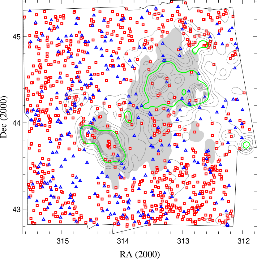
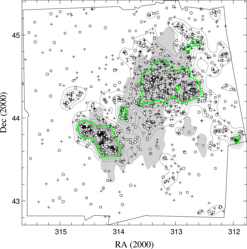
Figure 8.— TOP: the spatial distribution of background contaminants (red squares: AGN like sources, blue triangles: galaxies; see text and Figure 4). BOTTOM: the spatial distribution of YSO candidates, where symbols denote the object Class (circles: Class I or Flat, $+$: Class II, square: Class II-III). In both panels, we plot contours of YSO density (see text for more details); the contour levels correspond to values plotted in Figure 10, from 200 to 2000 YSOs/deg². The contour which surrounds half of the total YSO population ($\sim$1000 YSOs/deg²) is highlighted in green and with a thicker contour line. The background gray area indicates the $A_{V}\geq$5 dark cloud from the Cambrésy et al. (2002) map.

Now that we have a minimally contaminated sample of YSO candidates, we can look at their spatial distribution and investigate the degree of clustering and the relative spatial distribution of YSOs as a function of their class. We have computed a YSO density map of our observed region. We used a Kernel method (Silverman, 1986) which yields a smooth isodensity contour map from the projected position of objects. In each point of the space $(\alpha,\delta)$, the density is set, due to the contribution of all $n$ points, by the kernel density estimator:

$$D(\alpha,\delta)=\frac{1}{h^{2}}\sum_{i=1}^{n}K(\alpha,\alpha_{i},\delta,\delta_{i})$$

where $K$ is the kernel. For the kernel, we adopted a Gaussian shape :

$$K(\alpha,\alpha_{i},\delta,\delta_{i})=\frac{1}{2\pi}\exp{\frac{-\left((\delta-\delta_{i})^{2}+(\alpha-\alpha_{i})^{2}\cos^{2}\delta\right)}{2h^{2}}}$$

where $h$ is the smoothing parameter. We adopted $h=0.05\arcdeg$ (0.5 pc), which is approximately the size of the smallest group of YSOs in the NANeb discernible ‘by eye’.

Figure 8 shows contours of the density map we obtained, where both background contaminants and YSO candidates are plotted in two different panels. Using these density contours, we find first that the background contaminants (galaxies or AGN) are relatively evenly distributed across the field of view. However, we notice a lack of background contaminant sources on the central dark cloud. The lack of contaminants in the high extinction regions can be quantitatively explained simply due to the fact that our survey is magnitude-limited, and the extra extinction causes the observed fraction of galaxies to drop out of our sample. We checked this assumption by creating an artificial map of randomly distributed background sources reddened by the extinction map of Cambrésy et al. (2002). We then applied a magnitude cut to this artificial sample, corresponding to the effective faint limit imposed by our 4-band YSO selection criteria. The resulting spatial distribution of selected galaxies mimics well the observed galaxy distribution in Figure 7(top), confirming our assumption.

Our YSO candidates are located primarily on the central dark cloud (Lynds 935), and are for the most part highly clustered. Further, we find that half of our YSO population is located in regions denser than 1000 YSOs/deg² ($\sim$10⁵ YSOs/pc²) and cover a relatively small fraction of the sky ($\sim$0.5 deg² compared to the $\sim$9 deg² observed).

From the distribution of YSOs, we distinguished by eye 8 main clusters (for a discussion of more quantitative means to identify clusters of YSOs from similar catalogs, see for example Jorgensen et al. 2008). We determined the center of each cluster as the local peak of the YSO density. We arbitrarily define the boundaries of these clusters as the YSO density contour at a level of 1/4 of the maximum density peak. The location, the size, the number of stars and the mean $A_{v}$ for each cluster is provided in Table 3. Five of these clusters have been previously identified by Cambrésy et al. (2002); they are the most prominent clusters located inside the Gulf of Mexico and in the central part of the NANeb. Figure 9 shows the location of both our clusters and clusters defined by Cambrésy et al. One can see in this figure that cluster #4 of Cambrésy et al. (2002) does not exist in our YSO candidate distribution. Clusters #7 and #8 of Cambresy appear in our YSO distribution, but are similar to many other small clusters in the NANeb; they are not as densely populated as the ones we have defined. Because the Cambrésy et al. (2002) technique is sensitive to both WTTs and CTTs, whereas ours essentially excludes WTTs, it is reasonable that our two methods will yield somewhat different results. It is likely that the clusters found by Cambrésy et al. (2002) but not by us may be the evolutionarily older clusters in the region.

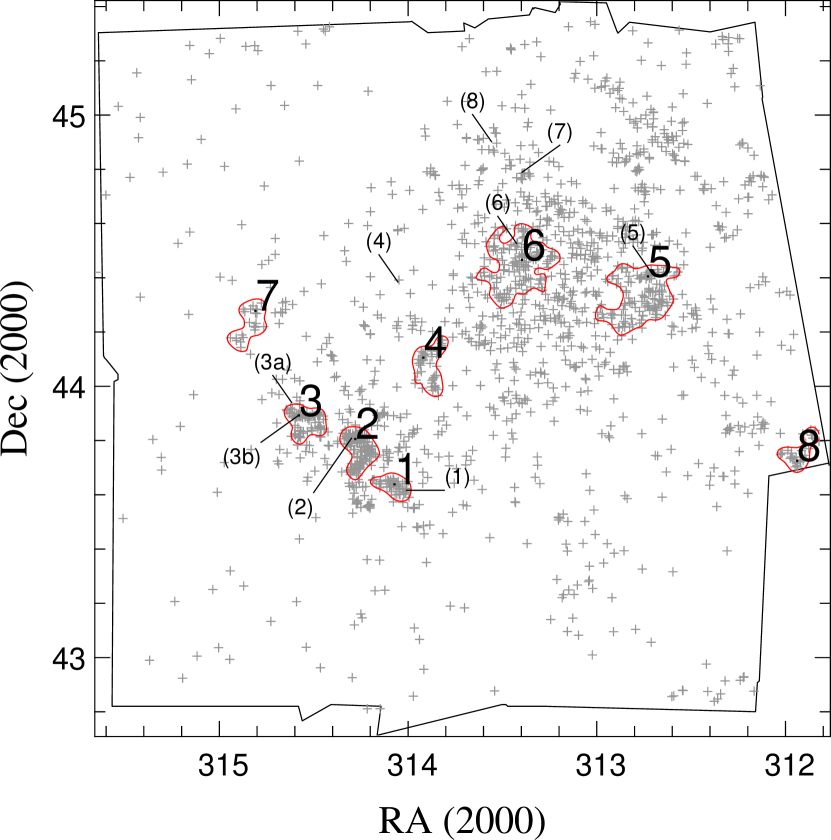
Figure 9.— Location of clusters shown on the distribution of the $\sim$1600 YSO candidates (plus symbols). Solid red lines are contours of clusters we adopted (see text for more details). Our eight clusters are labelled with large, bold numbers and no brackets. The location of clusters found by Cambrésy et al. (2002) are also indicated by smaller bracketed labels.

Table 3NANeb clusters

id	RA	Dec	Area	YSOs	$<A_{v}>$	idc
	J(2000)	J(2000)	deg2	Count	mag
1	20 56 17.4	+43 38 18.8	0.015	48	18.12	1
2	20 57 07.1	+43 48 21.8	0.025	120	16.47	2
3	20 58 19.0	+43 53 32.5	0.023	74	4.93	3b
4	20 55 40.5	+44 06 20.0	0.025	39	5.68	…
5	20 50 54.9	+44 24 18.1	0.067	121	5.54	5
6	20 53 35.2	+44 27 57.4	0.075	130	6.27	6
7	20 59 14.2	+44 16 41.3	0.022	22	1.48	…
8	20 47 45.1	+43 43 29.4	0.017	28	…	…

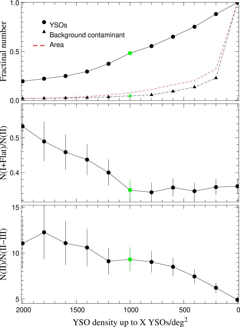
Figure 10.— Ratios of object classes as a function of YSO density. The $x$-axis corresponds to the YSO density contours plotted in Figure 8 from hight density to low density (corresponding to small and large surface surrounded by each contour on Figure 8). Inside each contour, we calculated several fractional numbers: TOP: the fraction of YSO candidates (filled dot symbols linked by solid line) and background contaminants (filled triangle liked by dot-dashed line); the red dashed line shows the surface area surrounded by each contour as a fraction of the total covered surface ($\sim$9 deg²) MIDDLE: same, but for the fraction of (Class I+Flat) / Class II. BOTTOM: same, but for the fraction of Class II / Class II-III. Note that for the last value, $X$=0 corresponds physically to the boundary of our IRAC coverage.

In the bottom panel of Figure 8, we plot the location of YSOs with different symbols corresponding to their class. To investigate in more detail a possible spatial segregation between Class I(+flat), II, and II-III, we used the YSO density contours to define regions within which we have computed the ratio of N(Class I + Flat) / N(Class II) and N(Class II) / N(Class II-III). The behavior of these ratios as a function of the density contour limit appears in Figure 10. This Figure shows that in dense regions (i.e., more clustered regions), the proportion of Class II objects compared to the (presumably) younger Class I’s is statistically lower than in the entire observed region by a factor of $\sim$1.3. This is consistent with expectations - either due to high velocity stars moving away from their birth sites, or as a result of the overall expansion of young clusters as they age due to, for example, removal of their remaining molecular cloud material by stellar winds. Moreover, the ratio N(Class II)/N(Class II-III) decreases from denser to less dense regions, as expected for the same reasons, by a factor of $\sim$2.

Figure 10 also shows the fractional number of background contaminants as compared to the fractional surface area inside each of the YSO density contours. The proportional number of background contaminants follows very closely the proportional surface area. This suggests that sources flagged as contaminants are really background objects and not YSOs; otherwise one would expect an excess of sources flagged as background inside dense regions.

Another way to characterize the degree of clustering, used by many authors, is the distribution of nearest neighbors. For each of our YSO candidates, we calculated the distance to the 4th nearest YSO candidates; Figure 11 shows the histogram of this distance, displayed for Class I+Flat, Class II and Class II-III. We find a statistically significant difference between the 3 histograms: using a Kolmogorov-Smirnov test, the probability that each of these distributions is drawn from the same parent distribution as either of the other two distributions is less than 0.02%. This is consistent with what we found above: the Class I population, usually assumed to be younger, is significantly more clustered than Class II-III.

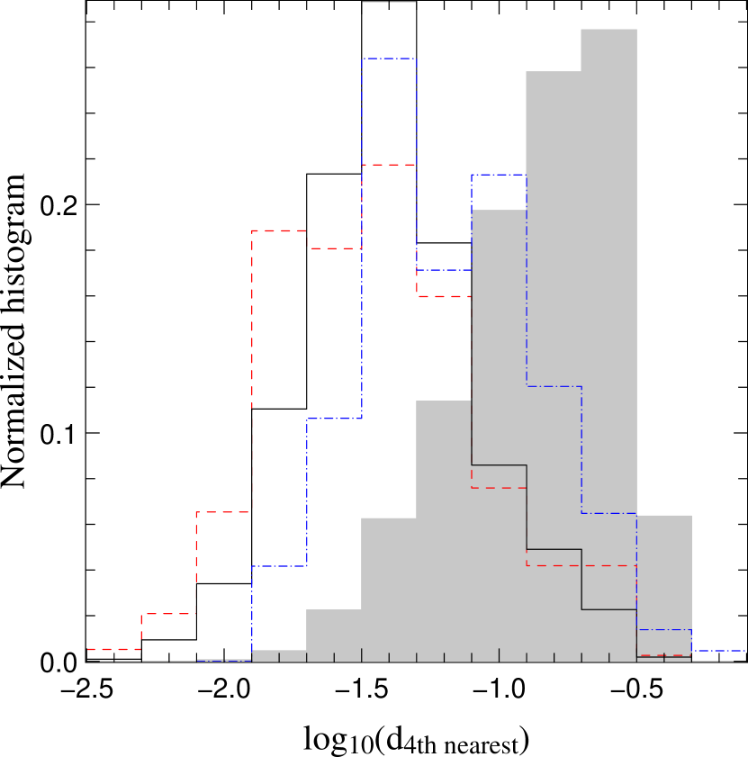
Figure 11.— Histogram of the log of the distance of the 4th nearest YSO (in degrees) for each of our YSO candidates. The red dashed line is for Class I+Flat spectrum sources, the solid black line for Class II stars and the blue dash-dot histogram for Class II-III. The gray histogram represents the remaining population of non-cluster members. The Class I population, usually assumed to be younger, is significantly more clustered than Class II-III; this is consistent with expectations that, as stars dynamically evolve, they move away from their birthplace.

4. HH Objects

Ogura et al. (2002) identified some HH objects using H$\alpha$ over a small region of the complex near bright-rimmed cloud (BRC) 31. Bally & Reipurth (2003) studied the entire Pelican Nebula using H$\alpha$, [N II], and [S II], finding several new HH objects.

The 3.5 to 8.5 $\mu$m wavelength range covered by the IRAC four channels is quite suitable to study deeply embedded young stellar outflows, since this range includes some of the brightest collisionally excited pure rotational H₂ emission lines (Wright et al., 1996; Noriega-Crespo et al., 2004a, b) as well as other H₂ vibrational lines (Smith & Rosen, 2005). At the longer wavelengths, the MIPS channels sample a rich combination of atomic/ionic and molecular lines that include some of the best atomic species to study outflows, e.g. [Fe II] 25.98 $\mu$m, [O I] 63.18 $\mu$m and [C II] 157.74 $\mu$m (see e.g. Molinari et al. 2000; Morris et al. 2004) that fall within the 24, 70 and 160 $\mu$m bandpasses, respectively, plus of course continuum emission from cold dust. We discuss below our observations of one HH object discovered previously, HH 555.

HH 555 itself is not an embedded flow (like e.g. HH 211) since it is clearly detected at optical wavelengths (H$\alpha$ and [S II] 6717/31 Å) and its spectrum is consistent with that of a shock excited gas moving supersonically (Bally & Reipurth, 2003). HH 555 belongs to that special class of irradiated jets, like HH 399 in the Trifid nebula (Yusef-Zadeh et al., 2005) that are found in active star forming regions and are surrounded by a bath of UV ionizing photons from recently formed massive stars.

The case for HH 555 is particularly interesting because the jet and counter-jet are bent westward as soon as they arise from their embedded source at the dense tip of the pillar, indicating the presence of stellar “sidewind” (Masciadri & Raga, 2001). The pillar itself is being photoevaporated leading to the formation of a two-shock structure (see Kajdič & Raga 2007 for details). The length of time that the jet will maintain its bipolar morphology is expected to depend on the strength of the impinging ionizing flux. The two-shock structure developed by the interacting winds actually creates a shield that protects both the jet and the pillar, and therefore, one would expect lower ionization on the West side of the outflow. Indeed, the Spitzer images combined with the ground based H$\alpha$ emission (Figure 12) confirms this stratification, if one assumes that the 8 $\mu$m and 24 $\mu$m emission arises mostly from H₂ and [S II], as is the case in other jets. This also explains why the 24 $\mu$m source lies in the middle of the 8 $\mu$m and 24 $\mu$m jets, but is slightly offset with respect to H$\alpha$ (see e.g. Kajdič & Raga 2007, Fig. 3).

Our 70 $\mu$m images do not show a clear signature of the jet, and this could be due to a combination of things: lack of sensitivity, artifacts along the scanning direction and physics ([O I] 63.18 $\mu$m is not present, neither is cold dust). Careful analysis of the data do show the presence of the source at 70 $\mu$m at the tip of the pillar. The pillar itself, although faint, is distinguished and its emission is likely to be due to [O I] photodissociated emission. We measured the flux at 24 and 70 $\mu$m using a small aperture of 7″ and 16″ respectively, centered at 20h51m19.52s +44d25m38.3s. We found 10$\pm$3 mJy at 24 $\mu$m and 830$\pm$220 mJy at 70 $\mu$m.

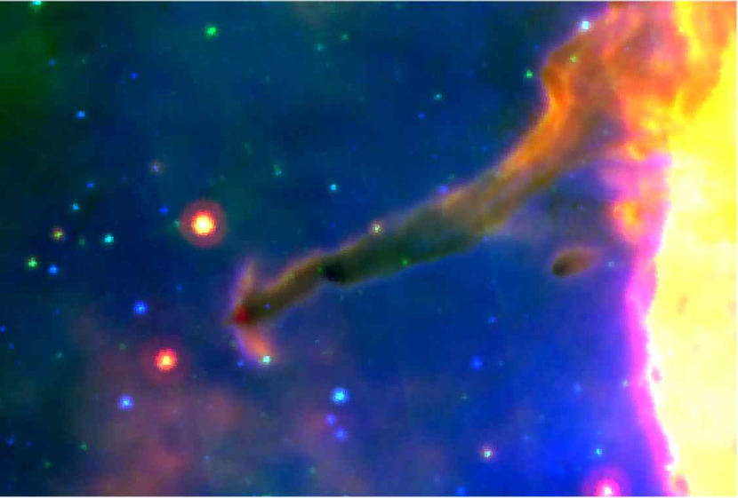
Figure 12.— Three color image of HH 555 arising from the tip of a dense pillar using H$\alpha$ (blue), IRAC 8 $\mu$m (green) and MIPS 24 $\mu$m (red). The FOV is $\sim 6\arcmin\times 4\arcmin$, and North is up and East is left. The mid/far infrared bipolar jet ($\sim$ 1′ in length) is centered on a 24 $\mu$m  embedded source. The stratification in ionization along the jet from East-to-West (the gradient in color) can be explained by the shield created during the two (stellar and photoevaporation) wind interaction (Kajdič & Raga, 2007).

5. Conclusion

We have combined mid-IR photometry from Spitzer/IRAC with $JHK_{s}$ data from 2MASS to provide a sensitive photometric census of objects towards the North America and Pelican Nebulae. We have used IRAC color and magnitude diagnostics to identify more than 1600 sources with infrared excess characteristic of young stars surrounded by a disk.

Our YSO candidates are located primarily on the central dark cloud (Lynds 935). We identified 8 main clusters, which together contain about a third of all the YSOs in the region; 5 of these clusters were previously recognized by Cambrésy et al. (2002). The sources we identify as background galaxies or AGN are relatively uniformly spread across the observed region. These two properties suggest a low level of contamination in our YSO sample.

We have assigned our YSOs classifications in the Class I/Flat/II/III system according to their infrared SED slope. The proportion of Class I+Flat compared to Class II is variable within the NANeb, with the dark clouds called “Gulf of Mexico” having a remarkably higher proportion of Class I’s, suggesting these clusters have a younger age than the rest of NANeb. The “Gulf of Mexico” region will be discussed in more detail in R09 where the MIPS data for NANeb will be presented.

We compared optical photometry of a small sample of the YSO candidates to evolutionary models in order to provide an age estimate for the NANeb. We found that most of these YSOs appear younger than 10 Myr according to the isochrones of Siess et al. (2000), with the median age being 3 Myr. However, the most embedded and probably youngest YSOs were not included in this sample because our optical photometry is less sensitive than our IRAC observations and because the youngest stars are very red. However, despite all the caveats regarding this age estimation, it is the most robust published so far.

Finally, thanks to our infrared images from 3.6 to 70 $\mu$m, we have provided new clues on the nature of HH 555, a peculiar HH object reported in Bally & Reipurth (2003). We detected a source at 70 $\mu$m at the base of the bi-polar jets. Our data add support to the hypothesis that the bent shape of HH 555 is a result of having the jet propagate in an environment with a stellar “sidewind”.

Table 4Table of YSO candidates

IAU Designation	RA (2000)	Dec (2000)	2MASS id	$B$	$V$	$I$	$J$	$H$	$K_{s}$	$[3.6]$	$[4.5]$	$[5.8]$	$[8.0]$	$[24]$
SST205659.3+434753.0	20 56 59.326	43 47 52.993	20565934+4347530	20.195	18.747	15.963	14.286	13.485	13.174	12.609	12.287	11.892	11.348	…
SST205646.8+434609.0	20 56 46.765	43 46 08.980	20564675+4346089	19.981	18.023	15.385	13.226	12.180	11.783	11.653	11.485	11.244	10.392	5.060

References

- André (1994) André, P. 1994, in The Cold Universe, ed. T. Montmerle, C. J. Lada, I. F. Mirabel, & J. Tran Thanh van, 179
- Armond et al. (2003) Armond, A. C., Reipurth, B., & Vaz, L. P. 2003, Bulletin of the Astronomical Society of Brazil, 23, 92
- Bally & Reipurth (2003) Bally, J. & Reipurth, B. 2003, AJ, 126, 893
- Bally & Scoville (1980) Bally, J. & Scoville, N. Z. 1980, ApJ, 239, 121
- Baraffe et al. (1998) Baraffe, I., Chabrier, G., Allard, F., & Hauschildt, P. H. 1998, A&A, 337, 403
- Cambrésy et al. (2002) Cambrésy, L., Beichman, C. A., Jarrett, T. H., & Cutri, R. M. 2002, AJ, 123, 2559
- Comerón & Pasquali (2005) Comerón, F. & Pasquali, A. 2005, A&A, 430, 541
- Fazio et al. (2004) Fazio, G. G., Hora, J. L., Allen, L. E., et al. 2004, ApJS, 154, 10
- Flaherty et al. (2007) Flaherty, K. M., Pipher, J. L., Megeath, S. T., et al. 2007, ApJ, 663, 1069
- Gutermuth et al. (2008) Gutermuth, R. A., Myers, P. C., Megeath, S. T., et al. 2008, ApJ, 674, 336
- Harvey et al. (2007a) Harvey, P., Merín, B., Huard, T. L., et al. 2007a, ApJ, 663, 1149
- Harvey et al. (2006) Harvey, P. M., Chapman, N., Lai, S.-P., et al. 2006, ApJ, 644, 307
- Harvey et al. (2007b) Harvey, P. M., Rebull, L. M., Brooke, T., et al. 2007b, ApJ, 663, 1139
- Herbig (1958) Herbig, G. H. 1958, ApJ, 128, 259
- Jeffries et al. (2007) Jeffries, R. D., Oliveira, J. M., Naylor, T., Mayne, N. J., & Littlefair, S. P. 2007, MNRAS, 376, 580
- Kajdič & Raga (2007) Kajdič, P. & Raga, A. C. 2007, ApJ, 670, 1173
- Lada (1987) Lada, C. J. 1987, in IAU Symp. 115: Star Forming Regions, ed. M. Peimbert & J. Jugaku, 1–17
- Laugalys & Straižys (2002) Laugalys, V. & Straižys, V. 2002, Baltic Astronomy, 11, 205
- Luhman et al. (2003) Luhman, K. L., Stauffer, J. R., Muench, A. A., et al. 2003, ApJ, 593, 1093
- Makovoz & Marleau (2005) Makovoz, D. & Marleau, F. R. 2005, PASP, 117, 1113
- Masciadri & Raga (2001) Masciadri, E. & Raga, A. C. 2001, AJ, 121, 408
- Molinari et al. (2000) Molinari, S., Noriega-Crespo, A., Ceccarelli, C., et al. 2000, ApJ, 538, 698
- Morris et al. (2004) Morris, P. W., Noriega-Crespo, A., Marleau, F. R., et al. 2004, ApJS, 154, 339
- Muench et al. (2007) Muench, A. A., Lada, C. J., Luhman, K. L., Muzerolle, J., & Young, E. 2007, AJ, 134, 411
- Noriega-Crespo et al. (2004a) Noriega-Crespo, A., Moro-Martin, A., Carey, S., et al. 2004a, ApJS, 154, 402
- Noriega-Crespo et al. (2004b) Noriega-Crespo, A., Morris, P., Marleau, F. R., et al. 2004b, ApJS, 154, 352
- Ogura et al. (2002) Ogura, K., Sugitani, K., & Pickles, A. 2002, AJ, 123, 2597
- Rebull et al. (2002) Rebull, L. M., Makidon, R. B., Strom, S. E., et al. 2002, AJ, 123, 1528
- Siess et al. (2000) Siess, L., Dufour, E., & Forestini, M. 2000, A&A, 358, 593
- Silverman (1986) Silverman, B. W. 1986, Density estimation for statistics and data analysis (Monographs on Statistics and Applied Probability, London: Chapman and Hall, 1986)
- Skrutskie et al. (2006) Skrutskie, M. F., Cutri, R. M., Stiening, R., et al. 2006, AJ, 131, 1163
- Smith & Rosen (2005) Smith, M. D. & Rosen, A. 2005, MNRAS, 357, 1370
- Stauffer (1996) Stauffer, J. R. 1996, in Astronomical Society of the Pacific Conference Series, Vol. 109, Cool Stars, Stellar Systems, and the Sun, ed. R. Pallavicini & A. K. Dupree, 305
- Werner et al. (2004) Werner, M. W., Roellig, T. L., Low, F. J., et al. 2004, ApJS, 154, 1
- Wright et al. (1996) Wright, C. M., Drapatz, S., Timmermann, R., et al. 1996, A&A, 315, L301
- Yusef-Zadeh et al. (2005) Yusef-Zadeh, F., Biretta, J., & Wardle, M. 2005, ApJ, 624, 246