Time-delay and Doppler tests of the Lorentz symmetry of gravity

Abstract

Modifications to the classic time-delay effect and Doppler shift in General Relativity (GR) are studied in the context of the Lorentz-violating Standard-Model Extension (SME). We derive the leading Lorentz-violating corrections to the time-delay and Doppler shift signals, for a light ray passing near a massive body. It is demonstrated that anisotropic coefficients for Lorentz violation control a time-dependent behavior of these signals that is qualitatively different from the conventional case in GR. Estimates of sensitivities to gravity-sector coefficients in the SME are given for current and future experiments, including the recent Cassini solar conjunction experiment.

I Introduction

At the present time, General Relativity (GR) remains the best known fundamental theory of gravity, describing all known classical gravitational phenomena. Experiments testing this theory spanning $90$ years have failed to detect any convincing deviations. Despite its continuing success, there remains widespread interest in pushing the limits of experimental tests of GR in order to find possible deviations. This is primarily motivated by the consensus that there exists a unified fundamental theory that successfully meshes GR with the Standard Model of particle physics. Such a theory may produce small deviations from GR that could manifest themselves in sensitive experiments.

One promising avenue of exploration involves searching for violations of the principle of local Lorentz symmetry cpt ; reviews , a foundation of GR. Candidate theories exist in which this symmetry principle may be broken, at least at observable energy scales. These scenarios include strings strings ; ks1 , noncommutative field theories nc , spacetime-varying fields spacetimevarying , quantum gravity qg , supersymmetric theories berger , random-dynamics models fn , multiverses bj , and brane-world scenarios brane .

A general theoretical framework for testing Lorentz symmetry in both gravitational and nongravitational scenarios has been developed and is called the Standard-Model Extension (SME) sme ; akgrav . The SME is an effective field theory that incorporates the known physics of the Standard Model and GR, while also including all possible Lorentz-violating terms cptviolation . The Lorentz-violating terms are constructed from Standard Model and gravitational fields and coefficients for Lorentz violation, which control the degree of the symmetry breaking.

One useful subset of the SME, called the minimal SME, contains the Lorentz-violating terms that dominate at low energies. The matter sector of the minimal SME has been explored in experimental studies involving light light ; light2 ; light3 ; light4 ; light5 , electrons electrons , protons and neutrons protneut , mesons mesons , muons muons , neutrinos neutrinos , and the Higgs higgs . Some nonminimal SME terms, including Lorentz-violating operators of higher mass dimension, have already been explored in the photon sector in Refs. nonmin . In addition, because of the similarities of spacetime torsion to certain types of Lorentz violation, experimental searches for SME coefficients have been used to place new torsion constraints torsion . A summary of the current experimental constraints on SME coefficients can be found in Ref. tables .

Studies of the curved spacetime generalization of the SME have recently begun. Within the setting of a general Riemann-Cartan spacetime, the dominant SME lagrangian terms in the matter and gravitational sector have been established akgrav . The matter sector of the SME couples to gravity via the spin connection and vierbein. In this scenario, some novel effects can occur that are controlled by certain matter sector coefficients which are unobservable in the flat spacetime limit tkgrav . In the pure-gravity sector, key experimental signals in the Riemann spacetime limit have been established qbkgrav . Experimental work constraining SME coefficients in the gravity sector has already begun with atom-interferometric gravimeters gravi , lunar laser ranging llr , Gravity Probe B gpb , and short-range gravity tests srg .

Of the classic tests of GR, the so-called fourth test, involving the measurement of the Shapiro time delay of light passing near a massive body shapiro , has recently gained attention. Improvements in two-way radio communication with deep-space satellites, such as the Cassini probe, make possible a reduction in solar corona noise, yielding significant improvements in the accuracy of such tests bit . Further improvement in both time-delay and light-bending tests is also expected in the future lator ; odyssey ; beacon ; astrod ; sims ; st1 ; bepicolombo . It is therefore relevant to analyze in some detail the signals for Lorentz violation in such experiments. Some preliminary results describing the leading Lorentz-violating corrections to the Shapiro time-delay effect were obtained in Ref. qbkgrav and were applied to the case of binary-pulsar timing experiments. We seek here to elaborate on these results, determine in addition the associated gravitational frequency shift signal, and study potential signals in solar-system experiments.

This paper is organized as follows. In Sec. II, we discuss the theoretical foundations of this work. Section II.1 reviews key results in the gravitational sector of the SME, including the post-newtonian metric. We discuss light propagation in a background spacetime in Sec. II.2, and apply the results to obtain the time-delay formula in Sec. II.3 and the frequency shift formula in Sec. II.4. In Sec. III, we examine the results in the solar-system scenario. Some preliminary discussion of the experimental scenario in Sec. III.1 is followed in Sec. III.2 by some exploration of the features of the Lorentz-violating signals in time-delay tests and Doppler tests. We discuss how analysis might proceed and estimate sensitivities for existing and future experiments in Sec. III.3. The main results of this work are summarized in Sec. IV. Throughout this work we adopt standard notation and conventions for the SME, as contained in Refs. sme ; akgrav ; qbkgrav . In particular, we work in natural units where $\hbar=c=1$ and with the metric signature $-+++$.

II Theory

II.1 Basics

The SME with gravitational and nongravitational couplings was presented in Ref. akgrav . The general scenario is a Riemann-Cartan spacetime and includes couplings to curvature and torsion degrees of freedom. We focus here on the pure-gravity sector in the Riemann spacetime limit, within the minimal SME case. The relevant action for this sector of the SME is written as

$$S = {{1}\over{16\pi G}}\int d^{4}x\sqrt{-g}[(1-u)R+s^{\mu\nu}R^{T}_{\mu\nu}$$ (1)

$$+t^{\kappa\lambda\mu\nu}C_{\kappa\lambda\mu\nu}]+S^{\prime}.$$

In this expression, $g$ is the determinant of the spacetime metric $g_{\mu\nu}$, $R$ is the Ricci scalar, $R^{T}_{\mu\nu}$ is the trace-free Ricci tensor, $C_{\kappa\lambda\mu\nu}$ is the Weyl conformal tensor, and $G$ is Newton’s gravitational constant. The 20 coefficients for Lorentz violation $u$, $s^{\mu\nu}$, and $t^{\kappa\lambda\mu\nu}$control the leading Lorentz-violating gravitational couplings. The additional piece of the action denoted $S^{\prime}$ contains the matter sector and possible dynamical terms governing the $20$ coefficients.

In the SME formalism, the action maintains general coordinate invariance, or observer diffeomorphism symmetry, as well as observer local Lorentz symmetry. However, because of the transformation properties of the coefficients for Lorentz violation, the SME action breaks both particle local Lorentz symmetry and particle diffeomorphism symmetry akgrav ; bkgrav . In the present context of the action in Eq. (1), the degree to which the particle symmetries are broken is controlled by the coefficients $u$, $s^{\mu\nu}$, and $t^{\kappa\lambda\mu\nu}$.

It has been demonstrated that explicit breaking of local Lorentz and diffeomorphism symmetry generally conflicts with the Bianchi identities of Riemann geometry akgrav . In the action (1) above, explicit symmetry breaking would correspond to specifying a priori the functional forms of the coefficients $u$, $s^{\mu\nu}$, and $t^{\kappa\lambda\mu\nu}$. If the Lorentz-symmetry breaking is dynamical, however, the conflict with Riemann geometry is avoided akgrav . In the latter scenario the coefficients for Lorentz violation are dynamical fields and satisfy their own equations of motion. This ensures that the Bianchi identities hold.

We consider here the case of spontaneous Lorentz violation. The dynamics governing the coefficients appearing in Eq. (1) are contained in the $S^{\prime}$ term. Through a dynamical process, the coefficient fields acquire vacuum expectation values that are denoted as $\overline{u}$, $\overline{s}^{\mu\nu}$, and $\overline{t}^{\kappa\lambda\mu\nu}$. For example, this may occur through the introduction of potential terms in $S^{\prime}$ for $u$, $s^{\mu\nu}$, and $t^{\kappa\lambda\mu\nu}$, whose minima are nonzero strings ; ks1 ; akgrav ; bkgrav ; bkmass . This scenario has been treated for the action in Eq. (1) in the linearized gravity limit, along with a broad study of signals for Lorentz violation in gravitational experiments, in Ref. qbkgrav . In particular, the post-newtonian metric was obtained, which comprises the starting point of this work. Note that models of spontaneous Lorentz-symmetry breaking, capable of producing the effective coefficients for Lorentz violation in (1), exist in the literature. These include scalar scalar , vector ks1 ; akgrav ; bkgrav ; bkmass ; bb ; ms , and two-tensor models cardinal .

To study the propagation of light signals in a weak-field gravitational system, such as the solar system, the dominant $O(2)$ contributions to the post-newtonian metric are needed PNorders . The relevant terms in the metric for the pure-gravity sector of the minimal SME are controlled by the coefficients $\overline{s}^{\mu\nu}$. They can be written in component form, in an asymptotically inertial post-newtonian coordinate system cartesian , as

$$g_{00} = -1+(2+3\overline{s}^{00})U+\overline{s}^{jk}U^{jk}+O(3),$$

$$g_{0j} = (a_{1}-2)\overline{s}^{0j}U-a_{1}\overline{s}^{0k}U^{jk}+O(3),$$

$$g_{jk} = \delta^{jk}+[2+(1-2a_{2})\overline{s}^{00}]\delta^{jk}U+2(a_{2}-1)\overline{s}^{jk}U$$

$$\hskip-19.0pt+[\overline{s}^{lm}\delta^{jk}-a_{2}\overline{s}^{jl}\delta^{km}-a_{2}\overline{s}^{kl}\delta^{jm}+2a_{2}\overline{s}^{00}\delta^{jl}\delta^{km}]U^{lm}.$$

In the limit of vanishing $\overline{s}^{\mu\nu}$ coefficients, the post-newtonian metric of GR is recovered. The potentials appearing in this metric are given for an arbitrary mass density $\rho$ by

$$U = G\int{{\rho(\vec{x}^{\prime},t)}\over{|\vec{x}-\vec{x}^{\prime}|}}d^{3}x^{\prime},$$

$$U^{jk} = G\int{{\rho(\vec{x}^{\prime},t)(x-x^{\prime})^{j}(x-x^{\prime})^{k}}\over{|\vec{x}-\vec{x}^{\prime}|^{3}}}d^{3}x^{\prime}.$$ (3)

In Eqs. (LABEL:metric), some coordinate gauge freedom remains in the two quantities $a_{1}$ and $a_{2}$. For example, the standard harmonic gauge can be obtained by setting $a_{1}=a_{2}=1$. We leave these quantities unspecified to explicitly display the gauge-dependent nature of some of the results we derive in this work. As discussed in detail elsewhere qbkgrav , the relationship between this metric and the standard Parametrized Post-Newtonian (PPN) metric cmw is one of partial overlap in a special isotropic limit of the SME.

We will consider in this work the post-newtonian metric that is produced by a massive body at rest at the origin of the chosen coordinate system. The dominant contributions to the potentials appearing in (LABEL:metric) are from the monopole terms. They depend on the coordinate position of the test body relative to the origin $r^{j}$. Thus we use

$$U = {{GM}\over{r}},$$

$$U^{jk} = {{GMr^{j}r^{k}}\over{r^{3}}},$$ (4)

where $M$ is the suitably defined mass of the central body. In (4), we have neglected higher multipoles, which can play a role in systematics kop ; st1 , and would be needed for a full treatment of the general relativistic time-delay and Doppler shift signals. For the present purposes, however, we need only the dominant contributions to these signals that are controlled by the $\overline{s}^{\mu\nu}$ coefficients.

If the mass of the central body is distributed significantly outwards from its center, then a substantial spherical moment of inertia can arise, as happens with the Earth. In this case, for a light signal grazing the surface of the central body, terms in the metric proportional to the moment of inertia $I$ of the body, as well those that might be produced from a quadrupole moment, can give a significant contribution to resulting signals controlled by the coefficients $\overline{s}^{\mu\nu}$ qbkgrav . For simplicity in this work, we neglect such cases and discard the metric terms dependent on $I$. This is not expected to produce a severe problem in typical solar-system experiments since it is known, in terms of the Sun’s mass $M$ and radius $R_{\odot}$, that $I_{\odot}\approx 0.059MR^{2}_{\odot}$ aa .

II.2 Light propagation

To find both the time-delay signal and the Doppler shift signal we employ standard methods and adopt the geometric optics limit of electrodynamics in curved spacetime mtw ; bg1 . We take the wave vector of a light ray, tangent to the light path $x^{\mu}(\lambda)$, to be

$$p^{\mu}={{dx^{\mu}}\over{d\lambda}},$$ (5)

where $\lambda$ is an affine parameter. Since the light ray is a null geodesic, it obeys the geodesic equation and the null vector condition given by

$${{dp^{\mu}}\over{d\lambda}} = -\Gamma^{\mu}_{\phantom{\mu}\alpha\beta}p^{\alpha}p^{\beta},$$

$$p^{\mu}p^{\nu}g_{\mu\nu} = 0.$$ (6)

Note that under these assumptions we are neglecting Lorentz violation in the photon sector of the SME, which in any case is tightly constrained compared to the gravitational sector light ; light2 ; light3 ; light4 ; light5 .

We first consider a one-way light signal sent from an event $E$ to an event $P$, that passes a central body. We will need to find the deviation of the light ray path in curved spacetime from the straight line path in Minkowski spacetime between the two events. The spatial endpoints of the path will be fixed at the two events $E$ and $P$, which amounts to solving (6) as a boundary-value problem rather than an initial-value problem.

To find the corrections due to curved spacetime we adopt a perturbative method using the linearized expansion for the metric and an expansion for the wave vector

$$g_{\mu\nu} = \eta_{\mu\nu}+h_{\mu\nu},$$

$$p^{\mu} = \overline{p}^{\mu}+\delta p^{\mu}.$$ (7)

Here $h_{\mu\nu}$ are the metric fluctuations, representing the deviation of $g_{\mu\nu}$ from the flat spacetime metric $\eta_{\mu\nu}$. The first term in the second equation is the zeroth-order wave vector that is constant and satisfies the condition $\eta_{\mu\nu}\overline{p}^{\mu}\overline{p}^{\nu}=0$. The second term $\delta p^{\mu}$ is the correction to the wave vector due to curved spacetime. Applying the null condition for the full wave vector $p^{\mu}$ to leading order in the metric perturbation $h_{\mu\nu}$ yields a constraint on $\delta p^{\mu}$:

$$2\overline{p}^{\mu}\delta p^{\nu}\eta_{\mu\nu}\approx-h_{\mu\nu}\overline{p}^{\mu}\overline{p}^{\nu}.$$ (8)

We shall denote the coordinates of the endpoint events $E$ and $P$ as $(t_{e},r_{e}^{j})$ and $(t_{p},r_{p}^{j})$, respectively. Generally in what follows, quantities referred to each of the events are denoted with subscripts $e$ and $p$. The zeroth-order spatial trajectory for the light ray will be a straight line in the direction $\vec{R}=\vec{r}_{p}-\vec{r}_{e}$. This implies that the zeroth-order wave vector, tangent to this straight line, has components $\overline{p}^{0}=1$ and $\overline{p}^{j}=\hat{R}^{j}$, where $\hat{R}=\vec{R}/R$ and $R=|\vec{R}|$. The zeroth-order spatial trajectory can be written as

$$x_{0}^{j}(\lambda)=\hat{R}^{j}\lambda+b^{j},$$ (9)

where $b^{j}$ is the impact parameter vector. It can be written as

$$b^{j}=r_{p}^{j}-\hat{R}^{j}\vec{r}_{p}\cdot\hat{R}.$$ (10)

Furthermore, to be consistent with the boundary conditions, the parameter $\lambda$ is taken to vary from $-l_{e}=\vec{r}_{e}\cdot\hat{R}$ to $l_{p}=\vec{r}_{p}\cdot\hat{R}$, from which it follows that $l_{e}+l_{p}=R$. The various quantities that we use to describe the zeroth-order trajectory of a light ray passing a central body are depicted in Fig. 1.

Figure 1: Diagram illustrating the meaning of the position vectors $\vec{r}_{p}$, $\vec{r}_{e}$, $\vec{R}$, and the impact parameter $\vec{b}$, for the zeroth-order light trajectory passing a massive body from events E to P.

The parametrization and definitions above have an immediate consequence on $\delta p^{j}$. Integration of the spatial components of the definition (5) over the light path, followed by use of the second equation in (7) yields

$$\int_{-l_{e}}^{l_{p}}\delta p^{j}d\lambda=0.$$ (11)

This result is just a reflection of the fact that the spatial endpoints of the trajectory are fixed. Equation (11) will be useful in deriving the light travel time formula and the Doppler shift formula, as we show below.

The corresponding integral involving the time component $\delta p^{0}$ does not vanish, however, on account of its being fixed by Eq. (8). In fact, it can be used to derive the light travel time. Integrating the time component of the definition (5) from $E$ to $P$, and making use of (8) and (11), we obtain

$$t_{p}-t_{e}=R+{{1}\over{2}}\int_{-l_{e}}^{l_{p}}h_{\mu\nu}\overline{p}^{\mu}\overline{p}^{\nu}d\lambda.$$ (12)

This equation forms the starting point for the derivation of the time-delay formula in Sec. II.3.

We now consider the shift in the frequency of light measured by two observers at the two events $E$ and $P$. The ratio of the frequencies $\nu$ measured at the two events can be obtained from the standard formula

$${{\nu_{P}}\over{\nu_{E}}}={{(U_{p}^{\mu}p_{\mu})_{P}}\over{(U_{e}^{\mu}p_{\mu})_{E}}},$$ (13)

where $U_{p}^{\mu}$ and $U_{e}^{\mu}$ are the four-velocities of two distinct observers present at events $P$ and $E$, respectively. Note that the quantities in the numerator and denominator are to be evaluated at the two events $P$ and $E$, as indicated.

To obtain an explicit expression for the frequency shift for the one-way trip past a massive body, it will be convenient to work with the covariant components of the wave vector $p_{\mu}=g_{\mu\nu}p^{\nu}$. Expanding Eq. (13) into space and time components yields

$${{\nu_{P}}\over{\nu_{E}}}=\left({{dt}\over{d\tau_{p}}}\right)\left({{d\tau_{e}}\over{dt}}\right)\left({{p_{0}+w^{j}p_{j}}\over{p_{0}+v^{j}p_{j}}}\right),$$ (14)

where $v^{j}$ and $w^{j}$ are the coordinate velocities of the two observers at events $E$ and $P$, and $\tau_{e}$ and $\tau_{p}$ are their proper times, respectively.

One convenient consequence of using the covariant wave vector is that, for a spacetime metric with no explicit time dependence, the component $p_{0}$ will be constant along the path of light $x^{\mu}(\lambda)$. Furthermore, this condition will be approximately true for the post-newtonian metric (LABEL:metric) from a massive body approximately at rest at the origin of the chosen post-newtonian coordinate system. Therefore we take

$${{dp_{0}}\over{d\lambda}}\approx 0.$$ (15)

It will be important, however, to determine what the constant $p_{0}$ is, in order to obtain the correct frequency shift result.

To determine the covariant components $p_{0}$ and $p_{j}$ of the wave vector in Eq. (14) we first expand in the manner of (7):

$$p_{\mu}=\overline{p}_{\mu}+\delta p_{\mu},$$ (16)

where $\overline{p}_{\mu}=\eta_{\mu\nu}\overline{p}^{\nu}$. Using the null constraint (6), Eq. (8), and the properties of $\overline{p}^{\mu}$, we can establish that

$$\delta p_{0} = -\hat{R}^{j}\delta p^{j}+h_{0\mu}\overline{p}^{\mu}-{{1}\over{2}}h_{\mu\nu}\overline{p}^{\mu}\overline{p}^{\nu},$$

$$\delta p_{j} = \delta p^{j}+h_{j\mu}\overline{p}^{\mu}.$$ (17)

If we integrate the constant $p_{0}=-1+\delta p_{0}$ over the light path, use the first equation in (17), and Eq. (11), we can establish that

$$\delta p_{0}={{1}\over{R}}\int_{-l_{e}}^{l_{p}}\left(h_{0\mu}\overline{p}^{\mu}-{{1}\over{2}}h_{\mu\nu}\overline{p}^{\mu}\overline{p}^{\nu}\right)d\lambda.$$ (18)

Furthermore, if we insert the expansion (16) into the geodesic equation (6), and integrate over the path we find

$$\delta p_{j}(P)-\delta p_{j}(E)={{1}\over{2}}\int_{-l_{e}}^{l_{p}}\partial_{j}h_{\mu\nu}\overline{p}^{\mu}\overline{p}^{\nu}d\lambda.$$ (19)

To find the value of $\delta p_{j}$ at the endpoints, which is needed to evaluate the frequency shift (14), we start with the expression (11). A suitable integration by parts, followed by the use of (19), yields the values of $\delta p_{j}$ at the two events $P$ and $E$ in terms of integrals of metric components:

$$\delta p_{j}(P) = {{1}\over{2R}}\int_{-l_{e}}^{l_{p}}[(\lambda+l_{e})\partial_{j}h_{\mu\nu}\overline{p}^{\mu}\overline{p}^{\nu}+2h_{j\mu}\overline{p}^{\mu})]d\lambda,$$

$$\delta p_{j}(E) = {{1}\over{2R}}\int_{-l_{e}}^{l_{p}}[(\lambda-l_{p})\partial_{j}h_{\mu\nu}\overline{p}^{\mu}\overline{p}^{\nu}+2h_{j\mu}\overline{p}^{\mu})]d\lambda.$$

The expressions (LABEL:depj4) and (18) form the starting point of the derivation of the Doppler shift in Sec. II.4. Note that, although we will focus in the next sections on the metric from the gravity sector of the minimal SME, the results (12), (14), (18), and (LABEL:depj4) could be applied to alternative theories of gravity in the linearized limit, with an approximately time-independent metric. In particular, though it lies beyond the scope of the present work, it would be of interest to investigate effects outside of the gravity sector of the minimal SME, such as matter-gravity couplings tkgrav . Finally, we note in passing that our results in Eqs. (LABEL:depj4) are consistent with Ref. bg1 .

II.3 Time-delay formula

To establish the one-way light travel time, which contains a time-delay term due to curved spacetime, we must evaluate the integral in Eq. (12). The projection of the metric along $\overline{p}^{\mu}$ that appears in the integrand can be written as

$$h_{\mu\nu}\overline{p}^{\mu}\overline{p}^{\nu}=\Delta U+\Delta^{jk}U^{jk}.$$ (21)

The quantities $\Delta$ and $\Delta^{jk}$ are given by

$$\Delta = 4+\overline{s}^{00}(4-2a_{2})+(2a_{1}-4)\overline{s}^{0j}\hat{R}^{j}$$

$$+2(a_{2}-1)\overline{s}^{jk}\hat{R}^{j}\hat{R}^{k},$$

$$\Delta^{jk} = 2\overline{s}^{jk}-a_{1}\overline{s}^{0j}\hat{R}^{k}-a_{1}\overline{s}^{0k}\hat{R}^{j}-a_{2}\overline{s}^{jl}\hat{R}^{l}\hat{R}^{k}$$ (22)

$$-a_{2}\overline{s}^{kl}\hat{R}^{l}\hat{R}^{j}+2a_{2}\hat{R}^{j}\hat{R}^{k}\overline{s}^{00}.$$

With these definitions the light travel time takes the form

$$t_{p}-t_{e}=R+{{1}\over{2}}\Delta\int^{l_{p}}_{-l_{e}}Ud\lambda+{{1}\over{2}}\Delta^{jk}\int^{l_{p}}_{-l_{e}}U^{jk}d\lambda.$$ (23)

Using the monopole expressions in Eq. (3), and evaluating the potentials with the zeroth-order spatial trajectory (9), these integrals can be evaluated by standard methods. The resulting expression for the one-way light travel time, to post-newtonian order $O(2)$, is given by

$$t_{p}-t_{e} = R+2GM(1+\overline{s}^{00}-\overline{s}^{0j}\hat{R}^{j})\ln\left[{{r_{e}+r_{p}+R}\over{r_{e}+r_{p}-R}}\right]$$ (24)

$$+GM[-a_{2}\overline{s}^{00}+a_{1}\overline{s}^{0j}\hat{R}^{j}+\overline{s}^{jk}\hat{b}^{j}\hat{b}^{k}$$

$$\phantom{M}+(a_{2}-1)\overline{s}^{jk}\hat{R}^{j}\hat{R}^{k}]\left({{l_{e}}\over{r_{e}}}+{{l_{p}}\over{r_{p}}}\right),$$

$$+GM[a_{1}\overline{s}^{0j}b^{j}+(a_{2}-2)\overline{s}^{jk}\hat{R}^{j}b^{k}]{{(r_{e}-r_{p})}\over{r_{e}r_{p}}}$$

$$+...,$$

where the ellipses represent higher order post-newtonian corrections. Neglecting these term suffices to establish the leading effects from Lorentz violation for experiments. Note that this one-way result matches that obtained in Ref. qbkgrav in the appropriate limit. Also, in the isotropic limit of the SME, and for the appropriate coordinate choice, the result (24) matches the standard PPN result mtw ; cmw .

In many practical cases, the light signal is reflected from a planet or spacecraft. Using (24) we can establish the round-trip light travel time. This involves adding the light travel time for a signal transmitted by an observer at event $P$ that travels to the other observer arriving at an event denoted $E^{\prime}$. The light travel time for the return trip can be obtained from (24) with the substitutions

$$\vec{r}_{e} \rightarrow \vec{r}_{p},$$

$$\vec{r}_{p} \rightarrow \vec{r}_{e}\,^{\prime},$$ (25)

where $\vec{r}_{e}\,^{\prime}$ is the position of event $E^{\prime}$. Note that the quantities $\vec{R}$ and $\vec{b}$ will change for the return trip accordingly. We assume that the observer at event $E$, later receiving the returned signal at event $E^{\prime}$, is traveling at small velocities compared to $1$. Thus it suffices to approximate the motion during the light transit as rectilinear. The small velocities are in any case implied by the post-newtonian expansion adopted here. If we account for this motion during the light transit, but we neglect terms of order $GMv$, the order $GM$ portion of the light travel time is equal to its value for the outgoing trip, except for sign changes in the $\overline{s}^{0j}$ terms. Thus we obtain for the round-trip light travel time

$$\Delta t \approx {{2R(1-\hat{R}\cdot\vec{v})}\over{1-v^{2}}}+4GM(1+\overline{s}^{00})\ln\left[{{r_{e}+r_{p}+R}\over{r_{e}+r_{p}-R}}\right]$$ (26)

$$+2GM[-a_{2}\overline{s}^{00}+\overline{s}^{jk}\hat{b}^{j}\hat{b}^{k}$$

$$\phantom{2GM}+(a_{2}-1)\overline{s}^{jk}\hat{R}^{j}\hat{R}^{k}]\left({{l_{e}}\over{r_{e}}}+{{l_{p}}\over{r_{p}}}\right)$$

$$+2GM(a_{2}-2)\overline{s}^{jk}\hat{R}^{j}b^{k}\left({{r_{e}-r_{p}}\over{r_{e}r_{p}}}\right).$$

Note that the terms with the $\overline{s}^{0j}$ coefficients canceled when adding the outgoing and return trip contributions. This is due to their oddness under parity.

Neglecting terms of order $GMv$, the measured elapsed proper time $\Delta\tau_{e}$ at the receiver is related to the above result by the factor $d\tau_{e}/dt$, which is to be evaluated along the worldline of the receiver. In principle, this factor contains contributions from the spacetime metric near the observer present at event $E$ and is related to the classic gravitational redshift as discussed in the next subsection. For our analysis in this work, we focus on effects from a single body stemming from the $O(GM)$ terms in the expression above, though the results could be generalized to $N$ bodies.

There are two key time scales which could be used to distinguish the large special-relativistic effects contained in the first term in (26) from the smaller terms of order $GM$ bg1 . The time scale over which significant changes occur with the first term is essentially an orbital time scale $\overline{r}/\overline{v}$, where $\overline{r}$ and $\overline{v}$ are typical orbital distances and velocities, respectively, comparable to $R$ and $v$ defined in Sec. II.2. The conjunction time scale $b/\overline{v}$ is approximately the time scale over which the $O(GM)$ terms in (26) vary significantly. For typical experiments this is on the order of days.

The dominant contribution from the $O(GM)$ terms comes from the logarithmic term in (26). Note that the only coefficient for Lorentz violation appearing in front of the logarithmic term is the rotational scalar $\overline{s}^{00}$, which points to the possibility of its being measured at the same level as the PPN parameter $\gamma$. Anisotropic coefficients control many of the remaining terms. As we show for specific experiments in Sec. III, the typical size of the remaining terms are somewhat suppressed relative to the logarithmic term.

It is important to note that, in principle, the special-relativistic terms in (26) also receive corrections due to the gravity-sector coefficients $\overline{s}^{\mu\nu}$. These corrections would arise through modifications to the orbital dynamics of the transmitting and reflecting bodies (e.g., Earth and spacecraft or planet). For the purposes of detailed modeling, these effects could be included, for example, by modeling the orbits as oscillating ellipses. Secular changes in the orbital elements due to the coefficients $\overline{s}^{\mu\nu}$ could be included using the results from Ref. qbkgrav . In any case, such orbital corrections are expected to be relevant over the orbital time scale $\overline{r}/\overline{v}$.

II.4 Frequency shift

In GR, in addition to the bending of light and the time-delay effect, the frequency of light also changes after having passed near a massive body shapiro66 . This effect, closely related to the time-delay effect, is distinct from the classic gravitational redshift and vanishes for stationary observers. In this section, we evaluate the one-way frequency shift, using the results of Sec. II.2, and also determine the fractional frequency shift for a two-way reflected signal.

We begin with Eq. (14), expanded to leading order in the wave vector shift $\delta p_{\mu}$:

$${{\nu_{P}}\over{\nu_{E}}}={{dt}\over{d\tau_{p}}}{{d\tau_{e}}\over{dt}}\left({{1-\delta p_{0}-w^{j}\hat{R}^{j}-w^{j}\delta p_{j}(P)}\over{1-\delta p_{0}-v^{j}\hat{R}^{j}-v^{j}\delta p_{j}(E)}}\right).$$ (27)

The result is expanded to all orders in velocity for the special-relativistic terms, but to $O(3)$ in the terms depending on the metric fluctuations $h_{\mu\nu}$. With some manipulation we obtain

$${{\nu_{P}}\over{\nu_{E}}}=\sqrt{{{1-\vec{v}^{2}}\over{1-\vec{w}^{2}}}}{{1-w^{j}\hat{R}^{j}}\over{1-v^{j}\hat{R}^{j}}}\left(1+\left({{\nu_{P}}\over{\nu_{E}}}\right)_{g}\right),$$ (28)

where the term arising from the effects of gravity via the metric fluctuations is labeled $g$ and is given by

$$\left({{\nu_{P}}\over{\nu_{E}}}\right)_{g}=\left({{\nu_{P}}\over{\nu_{E}}}\right)_{RS}+\left({{\nu_{P}}\over{\nu_{E}}}\right)_{D}.$$ (29)

The term labeled $RS$ on the right-hand side of (29) is the gravitational redshift. This term arises from the spacetime metric being evaluated at the endpoints of the light trajectory, namely events $E$ and $P$. It is given by

$$\left({{\nu_{P}}\over{\nu_{E}}}\right)_{RS} = \left(1+{{3}\over{2}}\overline{s}^{00}\right)GM{{r_{e}-r_{p}}\over{r_{e}r_{p}}}$$ (30)

$$+{{1}\over{2}}\overline{s}^{jk}GM\left({{r_{p}^{j}r_{p}^{k}}\over{r_{p}^{3}}}-{{r_{e}^{j}r_{e}^{k}}\over{r_{e}^{3}}}\right)+...,$$

where the ellipses represents higher post-newtonian corrections. Equation (30) includes leading Lorentz-violating corrections to the standard gravitational redshift of GR, which is recovered in the limit $\overline{s}^{\mu\nu}=0$. The result (30) would be of interest to investigate for gravitational redshift experiments, such as those incorporating sensitive atomic clocks on Earth or aboard orbiting satellites redshift ; cmw ; gps ; aces . Our main focus in this work, however, will be on the time-delay effect and its associated contribution to the frequency shift derived below.

The term labeled $D$ in Eq. (29) is the gravitational frequency shift of light due to the wave vector corrections $\delta p^{\mu}$, which reads

$$\left({{\nu_{P}}\over{\nu_{E}}}\right)_{D} = \delta p_{0}(v-w)^{j}\hat{R}^{j}-w^{j}\delta p_{j}(P)+v^{j}\delta p_{j}(E)$$

$$= {{1}\over{2R}}\int_{-l_{e}}^{l_{p}}\big{(}[\lambda(v-w)^{j}-l_{e}w^{j}-l_{p}v^{j})]\partial_{j}h_{\mu\nu}\overline{p}^{\mu}\overline{p}^{\nu}+(v-w)^{j}\hat{R}^{j}(2h_{0\mu}\overline{p}^{\mu}-h_{\mu\nu}\overline{p}^{\mu}\overline{p}^{\nu})+(v-w)^{j}h_{j\mu}\overline{p}^{\mu}\big{)}d\lambda.$$

This term represents a gravitational correction to the usual Doppler shift of Special Relativity. The integrals in (LABEL:fr5) can be evaluated by inserting the post-newtonian metric (LABEL:metric) and using the zeroth-order spatial trajectory of the light ray, in a manner similar to Sec. II.3. The result is significantly more cumbersome than (24), and so we adopt an approximation that is suitable for capturing the dominant terms that are proportional to the coefficients for Lorentz violation $\overline{s}^{\mu\nu}$. After evaluating the integrals in (LABEL:fr5), the results can be grouped according to powers of $(GM\overline{v}/b)(b/\overline{r})^{n}$. We will focus here on near-conjunction time scales where the dominant terms in (LABEL:fr5) are of order $GM\overline{v}/b$ and higher order terms will be suppressed by powers of the small factor $b/\overline{r}$.

Keeping only the order $GM\overline{v}/b$ terms, we obtain for the frequency shift contribution (LABEL:fr5),

$$\left({{\nu_{P}}\over{\nu_{E}}}\right)_{D}\approx{{4GM}\over{b}}[(1+\overline{s}^{00}-\overline{s}^{0j}\hat{R}^{j}+\overline{s}^{jk}\hat{b}^{j}\hat{b}^{k})\dot{b}-\overline{s}^{jk}\hat{b}^{j}\dot{b}^{k}].$$ (32)

In this expression the dot denotes a time derivative with respect to the post-newtonian coordinate time $t$. Note that the arbitrary quantities $a_{1}$ and $a_{2}$ keeping track of the coordinate gauge freedom have vanished in this result, indicating the coordinate invariance of (32). The result (32) can also be verified by taking the coordinate time derivative of (24) and using a known relationship between the frequency shift and light travel time shapiro66 .

The result (32) can be contrasted with the contributions to the frequency shift contained in the remaining terms in Eq. (28) and also (30). In the same manner as the special-relativistic terms in the light travel time expression (26), the velocity contributions in (28) and the gravitational terms in (30) will vary over the orbital time scale $\overline{r}/\overline{v}$ in typical experiments. In contrast, the signal in (32) will vary most significantly when the light ray passes near the central body ($b<<\overline{r}$), when the observers and the central body are in conjunction.

We now calculate the fractional frequency shift of a light signal reflected from the planet or spacecraft. Thus we seek

$${{\delta\nu}\over{\nu}}={{\nu^{\prime}-\nu}\over{\nu}},$$ (33)

where $\nu$ is the transmitted frequency and $\nu^{\prime}$ is the returned frequency. In a manner similar to what was done for the round-trip light travel time in Sec. II.3, we can obtain the frequency shift for the return signal with suitable substitutions in the one-way result (32). Adding the return signal to the outgoing one, we find that the gravitational portion of the leading fractional frequency shift from the round-trip signal is given by

$$\left({{\delta\nu}\over{\nu}}\right)_{g}={{8GM}\over{b}}[(1+\overline{s}^{00}+\overline{s}^{jk}\hat{b}^{j}\hat{b}^{k})\dot{b}-\overline{s}^{jk}\hat{b}^{j}\dot{b}^{k}]+...,\\$$ (34)

where the ellipses include terms of order $(GM\overline{v}/b)(b/\overline{r})$ and higher order post-newtonian corrections. Note that the $\overline{s}^{0j}$ terms have vanished due to their oddness under Parity, just as they did for the time-delay formula. Also, the time dependence of (34) is controlled by the behavior of the impact parameter vector $\vec{b}$ and its time derivative $\vec{\dot{b}}$.

III Experiments

In this section, the experimental implications of the results derived in Secs. II.3 and II.4 are examined in the context of key solar system experiments. We point out the basic features of the Lorentz-violating signals and contrast them with the GR case. Also, we describe how experiments could be used to probe various combinations of coefficients for Lorentz violation and estimate the level of sensitivity for each test.

III.1 Preliminaries

We work in a post-newtonian coordinate system that asymptotically coincides with the Sun-centered celestial-equatorial coordinate system adopted in most SME studies light4 . Space and time coordinates in this system are denoted with capital letters $(T,X^{J})$ scf . This approximation to an asymptotically inertial frame suffices for many SME experimental studies. Note that the Sun’s center is in orbit around the barycenter of the solar system with a mean velocity about $1000$ times smaller than the Earth’s orbital velocity. Standard practice in solar system experiments is to adopt the Barycentric Celestial Reference System. For our purposes here in identifying the leading Lorentz-violating effects, it suffices to proceed in the Sun-centered frame and neglect the Sun’s motion. However, in establishing beyond leading order corrections to the light travel time and Doppler observables in GR, the Sun’s velocity can play a role sunvel ; b07 .

To study the basic features of our results we focus on the solar conjunction time scale where the signals for Lorentz violation are near their maximum. In this scenario, where the light signal passes close to the Sun, we can assume approximately rectilinear motion for the Earth observer and the planet or spacecraft. The main changing variable in this case is the impact parameter vector bg1 ; bg2 . Assuming rectilinear motion, we expand the impact parameter vector around its minimum value $\vec{b}_{0}$ as

$$\vec{b}=\vec{b}_{0}+\dot{\vec{b}}_{0}T,$$ (35)

where $\dot{\vec{b}}_{0}$ is the time derivative of the impact parameter vector evaluated at the conjunction time $T=0$. Note that we also have $\vec{b}_{0}\cdot\dot{\vec{b}}_{0}=0$.

In many cases of interest, the time derivative of the impact parameter vector near the conjunction time can be written approximately as

$$\dot{\vec{b}}_{0}\approx{{l_{p}\vec{v}+l_{e}\vec{w}}\over{R}},$$ (36)

where $\vec{v}$ is the Earth receiver’s velocity and $\vec{w}$ is the velocity of the spacecraft or planet. All quantities on the right-hand side of Eq. (36) can be determined from their definitions in Sec. II.2 and are evaluated at $T=0$. Note that if the planet or spacecraft is many times further from the Sun than the Earth, so that $R>>l_{e}$ and $l_{p}\sim R$, the primary contribution to (36) is from the Earth’s velocity.

The approximations described above will serve our purposes in exploring the features of the Lorentz-violating time-delay and Doppler signals. However, as we discuss below in Sec. III.3, the more accurate results obtained in previous sections could be incorporated into a detailed computer code for a more rigorous approach. Furthermore, although we focus below on the case where the central body is the Sun, many of our results can also be applied to the case where the Earth or other bodies produce the gravitational time delay and frequency shift.

III.2 Time-delay and Doppler signals

Adopting the solar system scenario described above where the central massive body is the Sun, we can establish the general behavior of the time-delay formula. For definiteness, we adopt the post-newtonian coordinate gauge of Ref. qbkgrav , setting $a_{1}=a_{2}=1$. Though this gauge differs from the standard harmonic gauge at $O(3)$, for the $O(2)$ terms appearing in the time-delay expression it is equivalent. Also, for times near conjunction, the gauge-dependent terms in (26) will be either approximately constant or of order $GMb/\overline{r}$ or smaller, and hence negligible.

The dominant contributions to the two-way time delay can be written as

$$\Delta T_{g}\approx 4GM\left[(1+\overline{s}^{TT})\ln\left({{r_{e}+r_{p}+R}\over{r_{e}+r_{p}-R}}\right)+\overline{s}^{JK}\hat{b}^{J}\hat{b}^{K}\right].$$ (37)

To illustrate the different functional dependencies of the terms in Eq. (37) we make use of the approximate expression in (35). Up to constants, the expression for the time delay becomes

$$\Delta T_{g} \approx 4GM\Big{[}(1+\overline{s}^{TT})\ln\left({{4r_{e}r_{p}}\over{b^{2}_{0}+{\dot{b}}^{2}_{0}T^{2}}}\right)$$ (38)

$$+\overline{s}_{1}{{b^{2}_{0}}\over{b^{2}_{0}+{\dot{b}}^{2}_{0}T^{2}}}+\overline{s}_{2}{{2b_{0}{\dot{b}}_{0}T}\over{b^{2}_{0}+{\dot{b}}^{2}_{0}T^{2}}}\Big{]},$$

where $b_{0}=|\vec{b}_{0}|$ and ${\dot{b}}_{0}=|\dot{\vec{b}}_{0}|$. The two combinations of coefficients occurring in Eq. (38) are given by

$$\overline{s}_{1} = \overline{s}^{JK}(\hat{b}_{0}^{J}\hat{b}_{0}^{K}-\hat{\dot{b}}_{0}^{J}\hat{\dot{b}}_{0}^{K}),$$

$$\overline{s}_{2} = \overline{s}^{JK}\hat{b}_{0}^{J}\hat{\dot{b}}_{0}^{K},$$ (39)

where $\hat{\dot{b}}_{0}=\dot{\vec{b}}_{0}/{\dot{b}}_{0}$.

There are three functions that appear in expression (38). The first term contains the standard logarithmic dependence present in GR, which is scaled by the rotational scalar combination of coefficients $\overline{s}^{TT}=\overline{s}^{XX}+\overline{s}^{YY}+\overline{s}^{ZZ}$. The second and third terms are controlled by the anisotropic combinations of coefficients $\overline{s}_{1}$ and $\overline{s}_{2}$. To illustrate the typical behavior of the functions occurring in (38), we plot them in Fig. 2 for the case of the Cassini experiment which took place near the solar conjunction on June 21, 2002. For this plot, we adopt the approximate values $b_{0}=1.6R_{\odot}$, ${\dot{b}}_{0}=30\,{\rm km/s}$, and $GM/c^{2}=1.48\,{\rm km}$, where $R_{\odot}$ is the Sun’s radius.

Figure 2: The time-delay signals occurring in Eq. (38) near solar conjunction, plotted with the values for the Cassini experiment around June 21, 2002. The solid curve labeled GR gives the standard logarithmic dependence of GR, controlled by the combination $1+\overline{s}^{TT}$. The curves labeled lv1 and lv2 are the Lorentz-violating signals controlled by the combinations of coefficients $\overline{s}_{1}$ and $\overline{s}_{2}$, respectively.

The logarithmic dependence of the time-delay signal is well known from GR tdold . The two dashed curves in Fig. 2 represent departures from this standard behavior. In fact, part of the lv2 curve controlled by the combination of coefficients $\overline{s}_{2}$ produces an advancement of the light travel time rather than a delay. This may also occur with the lv2 curve controlled by the distinct combination of coefficients $\overline{s}_{1}$, if the overall sign of this combination is negative. The peak values of the lv1 and lv2 curves are about $20\mu{\rm s}$ in this example. Note that although we are effectively setting $\overline{s}_{1}=1$ and $\overline{s}_{2}=1$ for the purposes of plotting, no specific prediction is made here. As explained in the next subsection, these combinations of coefficients are expected to be much smaller than unity given current experimental constraints.

It is also interesting to study the frequency shift that corresponds to the time-delay signal. For two combinations of coefficients for Lorentz violation in the gravitational sector, this signal is enhanced over the time-delay signal. We examine the signal to $O(3)$ in the post-newtonian expansion and to leading order in $b/\overline{r}$, assuming near-conjunction times. From Eq. (34) the fractional frequency shift, expressed in the Sun-centered frame, is given by

$$\left({{\delta\nu}\over{\nu}}\right)_{g}={{8GM}\over{b}}[(1+\overline{s}^{TT}+\overline{s}^{JK}\hat{b}^{J}\hat{b}^{K})\dot{b}-\overline{s}^{JK}\hat{b}^{J}\dot{b}^{K}].$$

(40)

To see some of the features of the Lorentz-violating signals in (40), we use the approximate expression for the impact parameter vector (35). The expression for the gravitational fractional frequency shift becomes

$$\left({{\delta\nu}\over{\nu}}\right)_{g} \approx 8GM\Big{[}(1+\overline{s}^{TT}){{{\dot{b}}^{2}_{0}T}\over{b^{2}_{0}+{\dot{b}}^{2}_{0}T^{2}}}$$

$$+\overline{s}_{1}{{{\dot{b}}^{2}_{0}b^{2}_{0}T}\over{(b^{2}_{0}+{\dot{b}}^{2}_{0}T^{2})^{2}}}+\overline{s}_{2}{{b_{0}{\dot{b}}_{0}({\dot{b}}^{2}_{0}T^{2}-b^{2}_{0})}\over{(b^{2}_{0}+{\dot{b}}^{2}_{0}T^{2})^{2}}}\Big{]}.$$

Figure 3: The gravitational fractional frequency shift in Eq. (40) near solar conjunction, plotted with the values for the Cassini experiment around June 21, 2002. The solid curve labeled GR gives the standard ${\dot{b}}/b$ dependence of GR, controlled by the combination $1+\overline{s}^{TT}$. The curves labeled lv1 and lv2 are the Lorentz-violating signals controlled by the combinations of coefficients $\overline{s}_{1}$ and $\overline{s}_{2}$, respectively.

Just as in the time-delay case, three functions appear. We plot these functions in Fig. 3, again using values from the Cassini experiment and setting $\overline{s}_{1}=1$ and $\overline{s}_{2}=1$. The odd functional dependence of the signal controlled by the combination $1+\overline{s}^{TT}$ is known shapiro ; bg1 ; bit . The signal controlled by $\overline{s}_{1}$ resembles the GR case, though its peak size is reduced. The even functional dependence of the $\overline{s}_{2}$ signal is qualitatively different from the GR case. Note also that the maximum amplitude for this curve, which occurs at the conjunction time, is about twice that of the peak value for the GR curve. Also, as one can see qualitatively for each of the curves in Figs. 3 and 2, the Doppler signal is the negative of the time derivative of the time-delay signal shapiro66 .

III.3 Experimental analysis

We discuss here key aspects of the experimental analysis of the time-delay and Doppler signals for Lorentz violation in Eqs. (37) and (40). Also, we make sensitivity estimates for some key experiments.

A ubiquitous feature of signals for Lorentz violation is the orientation dependence of observable signals light4 ; qbkgrav . Gravitational time-delay and Doppler tests provide no exception to this rule. In particular, the combinations of coefficients $\overline{s}_{1}$ and $\overline{s}_{2}$, controlling the lv1 and lv2 signals in Figs. 2 and 3, depend on the conjunction orientation of the experiment. To illustrate this, we include a sketch of the orientation of a typical experiment at the time of conjunction in Fig. 4. This figure is oriented with the Sun-centered frame $Z$ axis upwards, while $\vec{r}_{e}$ points in the ecliptic to the Earth’s position. For experiments where the light signal comes within a few solar radii of the Sun, the spacecraft or planet position $\vec{r}_{p}$ is only slightly inclined to the ecliptic.

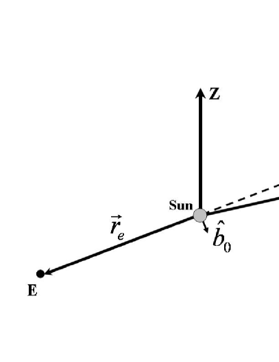
Figure 4: Diagram illustrating the conjunction configuration of a typical time-delay or Doppler experiment in the solar system. The Sun-centered frame $Z$ axis is shown along with the ecliptic plane (dashed line).

As an example of this orientation dependence, consider the Cassini experiment in 2002. Near the time of conjunction, the Earth’s velocity was pointing approximately along the Sun-centered frame $X$ axis (i.e., the vernal equinox direction). Furthermore $\hat{b}_{0}$ was pointing very nearly perpendicular to the ecliptic. In this case the plane of the illustration in Fig. 4 corresponds to the $YZ$ plane with the $X$ axis pointing out of the page. For this configuration we have

$$\hat{\dot{b}}_{0} \approx (1,0,0),$$

$$\hat{b}_{0} \approx (0,0.4,-0.9).$$ (42)

This implies that the Cassini experiment is sensitive to the combinations of coefficients

$$\overline{s}_{1} \approx 0.2\overline{s}^{YY}+0.8\overline{s}^{ZZ}-0.7\overline{s}^{YZ}-\overline{s}^{XX},$$

$$\overline{s}_{2} \approx 0.4\overline{s}^{XY}-0.9\overline{s}^{XZ}.$$ (43)

As another example, we suppose that the solar conjunction with the planet or spacecraft occurs near the vernal equinox. If this is the case, and the spacecraft or planet is much further away from the Sun than the Earth and slightly above the $XY$ plane, we have

$$\hat{\dot{b}}_{0} \approx (0,-1,0),$$

$$\hat{b}_{0} \approx (0,0,1).$$ (44)

The Sun-centered frame coefficients for this scenario are given by

$$\overline{s}_{1} \approx (\overline{s}^{ZZ}-\overline{s}^{YY}),$$

$$\overline{s}_{2} \approx -\overline{s}^{YZ}.$$ (45)

Due to its scaling of the GR results in both the time-delay and Doppler signals, the rotational scalar combination of coefficients $\overline{s}^{TT}$ is likely to be constrained at the same level as the PPN parameter $\gamma$, namely, parts in $10^{5}$. However, care is required since $\overline{s}^{TT}$ and $\gamma$ are not equivalent. In fact, the determination of the constant $GM$ may correlate with $\overline{s}^{TT}$. This is because $\overline{s}^{TT}$ occurs at $O(2)$ in Newtonian gravity qbkgrav . For example, in orbital dynamics in the presence of $\overline{s}^{\mu\nu}$ coefficients for Lorentz violation, the basic Newtonian acceleration between two bodies is scaled by $1+5\overline{s}^{TT}/3$. If orbits are described as ellipses with time-dependent orbital elements arising from perturbations to Newtonian gravity, the measured value $(GM)_{meas}=n^{2}a^{3}$, where $n$ is the orbital frequency and $a$ is the semimajor axis. Due to the presence of the $\overline{s}^{TT}$ coefficients $(GM)_{meas}=GM(1+5\overline{s}^{TT}/3)$. We therefore caution the reader that care is generally required in extracting constraints on $\overline{s}^{TT}$.

To fit experimental data to the Lorentz-violating time-delay and Doppler signals, one could proceed by at least two methods. First, having already fit data to a GR signal, one could extract constraints on SME coefficients from time-delay or Doppler residuals. This could be accomplished by using either the round-trip time-delay and Doppler formulas (40) and (37) or the less accurate versions (LABEL:freq4) and (38). As mentioned before, one must bear in mind that the coefficients for Lorentz violation $\overline{s}^{\mu\nu}$ also affect orbital dynamics. The effects on the orbits of the planets due to the gravity-sector coefficients can be described as secular changes over orbital time scales, although oscillations can also occur qbkgrav . However, these effects could in principle be avoided with suitable filtering of the data if the focus is on the conjunction time scale $b/\overline{v}$.

Alternatively, detailed modeling of the time-delay signal and the relevant orbital dynamics could be undertaken. In this case, the one-way formula in Eq. (24), which is valid to $O(2)$ in the post-newtonian expansion and for times far from conjunction, could be used appropriately for both uplink and downlink. The full post-newtonian equations of motion for the Earth and spacecraft or planet, and other relevant bodies that include the effects of the coefficients for Lorentz violation $\overline{s}^{\mu\nu}$ qbkgrav , could be incorporated into the Orbital Determination Program odp . Indeed, data from past experiments using radar reflection from the inner planets tdold ; inner could be reanalyzed to search for SME coefficients via this second method described above. Although many of these past experiments lack data near conjunction, when the Lorentz-violating signals controlled by $\overline{s}_{1}$ and $\overline{s}_{2}$ are peaked, they could still be useful in measuring the rotational scalar combination $\overline{s}^{TT}$. Furthermore, detailed modeling may also reveal suppressed dependencies of the time-delay signal on combinations of $\overline{s}^{\mu\nu}$ coefficients distinct from $\overline{s}_{1}$ and $\overline{s}_{2}$.

Regardless of the method adopted, we can make some reasonable estimates of the sensitivities achievable in experiments. We provide in Table 1 estimated sensitivities to the $3$ dominant combinations of coefficients in the time-delay and Doppler experiments for some past and future experiments. We include the Cassini experiment and some key future tests. The estimates are order of magnitude only and are based on the peak values of the Lorentz-violating signals discussed above and the approximate accuracy of each experiment referenced, when available. For example, the peak value of the $\overline{s}_{2}$ Doppler signal for the Cassini experiment is about $10^{-9}$, while the Allan deviation for this experiment is about $10^{-14}$ bit , indicating a sensitivity of parts in $10^{5}$. However, data from the time period when the $\overline{s}_{2}$ signal peaked in the 2002 conjunction ($T\approx 0$ in Fig. 3) is not available, so the sensitivity to $\overline{s}_{2}$ is more likely to be parts in $10^{4}$. On the other hand, it appears likely that a suitable fitting of Cassini data could place the first constraints on the rotational scalar combination $\overline{s}^{TT}$ at the $10^{-5}$ level. For the time-delay signals, the sensitivity to the $\overline{s}_{1}$ and $\overline{s}_{2}$ coefficients is reduced by about a factor of $10$ or more, as indicated in Fig. 2, and this reduction in sensitivity is included in Table 1.

Experiment	$\overline{s}^{TT}$	$\overline{s}_{1}$	$\overline{s}_{2}$	Ref.
Time-delay signal
Cassini	$10^{-5}$	$10^{-3}$	$10^{-4}$	bit
Odyssey	$10^{-7}$	$10^{-6}*$	$10^{-6}*$	odyssey
ASTROD	$10^{-8}$	$10^{-7}*$	$10^{-7}*$	astrod
BEACON	$10^{-9}$	$10^{-8}*$	$10^{-8}*$	beacon
Doppler signal
Cassini	$10^{-5}$	$10^{-4}$	$10^{-4}$	bit
Odyssey	$10^{-7}$	$10^{-7}*$	$10^{-7}*$	odyssey

Table 1: Crude estimates of attainable sensitivities in some key experiments for the time-delay and Doppler signals.

Proposals have been put forth for future experiments that measure to impressive accuracies the time delay from the Sun and even the Earth. We have included sensitivity estimates for the Odyssey, ASTROD, and BEACON experiments in Table 1. Although in some cases it may be difficult to directly measure the fractional frequency shift b07 , nonetheless we include some estimates in the table because of the possibility of increased sensitivity to SME coefficients from the Doppler signal over the time-delay signal. The experiments in Table 1 are by no means an exhaustive list. Also of possible interest are proposals for measuring the light-bending effect such as SIM sims and LATOR lator , other proposed experiments bepicolombo ; gaia , as well as existing accumulated data from Earth satellites gps . Though it lies beyond the scope of the present work, it would also be of interest to obtain the corresponding light-bending signal controlled by the $\overline{s}^{\mu\nu}$ coefficients.

Note that current constraints on the off diagonal components $\overline{s}^{XY}$, $\overline{s}^{YZ}$, and $\overline{s}^{XZ}$ are at the level of $10^{-8}$ from atom interferometry gravi . Two combinations of these and other $\overline{s}^{JK}$ coefficients are also constrained by lunar laser ranging at the $10^{-10}$ level llr . Thus, if future experiments can measure the peak behavior of the $\overline{s}_{2}$ set of coefficients in the Doppler signal to better than parts in $10^{8}$, they may produce measurements of coefficients competitive with or better than previous experiments. The $*$ label next to the estimated sensitivities in Table 1 indicates the requirement of measuring the peak behavior of the time-delay and Doppler signals. Finally we note that the $\overline{s}^{TT}$ coefficient does not appear at leading order in laboratory and orbital tests qbkgrav and so time-delay and Doppler tests are likely to be among the most sensitive to this coefficient.

IV Summary

In this work, we have analyzed Lorentz-violating corrections to the gravitational time-delay and Doppler signals in General Relativity, in the context of the gravitational sector of the minimal SME. We established general integral formulas for the deviation of a light ray from a straight line path that are valid in the linearized gravity limit. Our main results are analytical formulas for the light travel time and frequency shift for a light signal sent between two observers past a massive central body in the presence of gravity sector coefficients $\overline{s}^{\mu\nu}$. We obtained the one-way results in Eqs. (24) and (32) and the round-trip signals in Eqs. (26) and (34).

The Lorentz-violating signals were studied for solar system experiments involving light signals sent between the Earth and a planet or spacecraft near solar conjunction. It was determined that the dominant signals are controlled by the combinations of coefficients $1+\overline{s}^{TT}$, $\overline{s}_{1}$, and $\overline{s}_{2}$. In terms of Sun-centered frame coefficients, the combinations $\overline{s}_{1}$ and $\overline{s}_{2}$ will vary for different experiments. We obtained sensitivity estimates for key existing and future experiments which are summarized in Table 1. Time-delay and Doppler experiments could prove crucial in measuring the elusive scalar coefficient $\overline{s}^{TT}$, to better than parts in $10^{5}$. Future highly sensitive time-delay and Doppler tests may be able to measure other coefficients in the subset $\overline{s}^{JK}$ with sensitivities competitive with other existing experiments.

References

- (1) For recent conference proceedings on theoretical and experimental aspects, see V.A. Kostelecký, ed., CPT and Lorentz Symmetry IV, World Scientific, Singapore, 2008; CPT and Lorentz Symmetry III, World Scientific, Singapore, 2005; CPT and Lorentz Symmetry II, World Scientific, Singapore, 2002; CPT and Lorentz Symmetry, World Scientific, Singapore, 1999.
- (2) D.M. Mattingly, Living Rev. Relativity 8, 5 (2005); R. Bluhm, Lect. Notes Phys. 702, 191 (2006); arXiv:hep-ph/0506054v1.
- (3) V.A. Kostelecký and S. Samuel, Phys. Rev. Lett. 63, 224 (1989); V.A. Kostelecký and R. Potting, Nucl. Phys. B 359, 545 (1991).
- (4) V.A. Kostelecký and S. Samuel, Phys. Rev. D 40, 1886 (1989).
- (5) I. Mocioiu, et al., Phys. Lett. B 489, 390 (2000); S.M. Carroll et al., Phys. Rev. Lett. 87, 141601 (2001); Z. Guralnik et al., Phys. Lett. B 517, 450 (2001); C.E. Carlson et al., Phys. Lett. B 518, 201 (2001); A. Anisimov et al., Phys. Rev. D 65, 085032 (2002); A. Das et al., Phys. Rev. D 72, 107702 (2005); A.F. Ferrari et al., Phys. Lett. B 652, 174 (2007).
- (6) V.A. Kostelecký et al., Phys. Rev. D 68, 123511 (2003); R. Jackiw and S.-Y. Pi, Phys. Rev. D 68, 104012 (2003); N. Arkani-Hamed et al., JHEP 0405, 074 (2004).
- (7) J. Alfaro, H.A. Morales-Técotl, and L.F. Urrutia, Phys. Rev. D 66, 124006 (2002); D. Sudarsky et al., Phys. Rev. Lett. 89, 231301 (2002); Phys. Rev. D 68, 024010 (2003); G. Amelino-Camelia, Mod. Phys. Lett. A 17, 899 (2002); R. Myers and M. Pospelov, Phys. Rev. Lett. 90, 211601 (2003); N.E. Mavromatos, Lect. Notes Phys. 669, 245 (2005).
- (8) M.S. Berger and V.A. Kostelecký, Phys. Rev. D 65, 091701 (2002); M.S. Berger, Phys. Rev. D 68, 115005 (2003).
- (9) C.D. Froggatt and H.B. Nielsen, arXiv:hep-ph/0211106.
- (10) J.D. Bjorken, Phys. Rev. D 67, 043508 (2003).
- (11) C.P. Burgess et al., JHEP 0203, 043 (2002); A.R. Frey, JHEP 0304, 012 (2003); J. Cline and L. Valcárcel, JHEP 0403, 032 (2004); D.S. Gorbunov and S.M. Sibiryakov, JHEP 0509, 082 (2005); F. Ahmadi et al., Class. Quant. Grav. 23, 4069 (2006).
- (12) V.A. Kostelecký and R. Potting, Phys. Rev. D 51, 3923 (1995); D. Colladay and V.A. Kostelecký, Phys. Rev. D 55, 6760 (1997); Phys. Rev. D 58, 116002 (1998).
- (13) V.A. Kostelecký, Phys. Rev. D 69, 105009 (2004).
- (14) The SME also includes general CPT violation.
- (15) J. Lipa et al., Phys. Rev. Lett. 90, 060403 (2003); M. Tobar et al., Phys. Rev. A 72, 066101 (2005); P. Antonini et al., Phys. Rev. A 72, 066102 (2005); S. Herrmann et al., Phys. Rev. Lett. 95, 150401 (2005); P.L. Stanwix et al., Phys. Rev. D 74, 081101 (2006); J.P. Cotter and B.T.H. Varcoe, physics/0603111; H. Müller et al., Phys. Rev. Lett. 99, 050401 (2007); S. Reinhardt et al., Nature Physics 3, 861 (2007).
- (16) V.A. Kostelecký and A.G.M. Pickering, Phys. Rev. Lett. 91, 031801 (2003); R. Lehnert and R. Potting, Phys. Rev. Lett. 93, 110402 (2004); Phys. Rev. D 70, 125010 (2004); T. Jacobson et al., Phys. Rev. Lett. 93, 021101 (2004); B. Altschul, Phys. Rev. D 70, 056005 (2004); Phys. Rev. D 72, 085003 (2005); Phys. Rev. Lett. 96, 201101 (2006); F.R. Klinkhamer and C. Rupp, Phys. Rev. D 72, 017901 (2005); M.A. Hohensee et al., Phys. Rev. Lett. 102, 170402 (2009); arXiv:0809.3442; B. Altschul, arXiv:0905.4346.
- (17) S.M. Carroll, G.B. Field, and R. Jackiw, Phys. Rev. D 41, 1231 (1990); V.A. Kostelecký and M. Mewes, Phys. Rev. Lett. 87, 251304 (2001); Phys. Rev. Lett. 97, 140401 (2006).
- (18) V.A. Kostelecký and M. Mewes, Phys. Rev. D 66, 056005 (2002).
- (19) Q.G. Bailey and V.A. Kostelecký, Phys. Rev. D 70, 076006 (2004); M. Mewes, Phys. Rev. D 78, 096008 (2008).
- (20) H. Dehmelt et al., Phys. Rev. Lett. 83, 4694 (1999); R. Mittleman et al.Phys. Rev. Lett. 83, 2116 (1999); G. Gabrielse et al., Phys. Rev. Lett. 82, 3198 (1999); R. Bluhm et al., Phys. Rev. Lett. 79, 1432 (1997); 82, 2254 (1999); Phys. Rev. D 57, 3932 (1998); R. Bluhm and V.A. Kostelecký, Phys. Rev. Lett. 84, 1381 (2000); H. Müller et al., Phys. Rev. D 68, 116006 (2003); 70, 076004 (2004); L.-S. Hou, W.-T. Ni, and Y.-C.M. Li, Phys. Rev. Lett. 90, 201101 (2003); H. Müller, Phys. Rev. D 71, 045004 (2005); D. Colladay and P. McDonald, Phys. Rev. D 73, 105006 (2006); B. Heckel et al., Phys. Rev. Lett. 97, 021603 (2006).
- (21) V.A. Kostelecký and C.D. Lane, Phys. Rev. D 60, 116010 (1999); J. Math. Phys. 40, 6245 (1999); L.R. Hunter et al., in CPT and Lorentz Symmetry, Ref. cpt ; D. Bear et al., Phys. Rev. Lett. 85, 5038 (2000); D.F. Phillips et al., Phys. Rev. D 63, 111101 (2001); M.A. Humphrey et al., Phys. Rev. A 68, 063807 (2003); R. Bluhm et al., Phys. Rev. Lett. 88, 090801 (2002); Phys. Rev. D 68, 125008 (2003); F. Canè et al., Phys. Rev. Lett. 93, 230801 (2004); C.D. Lane, Phys. Rev. D 72, 016005 (2005); P. Wolf et al., Phys. Rev. Lett. 96, 060801 (2006); B. Altschul, Astropart. Phys. 28, 380 (2007); Phys. Rev. D 78, 085018 (2008); Phys. Rev. D 79, 016004 (2009); Phys. Rev. D 79, 061702 (R) (2009).
- (22) V.A. Kostelecký, Phys. Rev. Lett. 80, 1818 (1998); Phys. Rev. D 61, 016002 (1999); Phys. Rev. D 64, 076001 (2001); V.A. Kostelecký and A. Roberts, Phys. Rev. D 63, 096002 (2001); H. Nguyen (KTeV Collaboration), arXiv:hep-ex/0112046; FOCUS Collaboration, J.M. Link et al., Phys. Lett. B 556, 7 (2003); BaBar Collaboration, B. Aubert et al., Phys. Rev. Lett. 100, 131802 (2008); B. Altschul, Phys. Rev. D, 77, 105018 (2008).
- (23) R. Bluhm et al., Phys. Rev. Lett. 84, 1098 (2000); V.W. Hughes et al., Phys. Rev. Lett. 87, 111804 (2001).
- (24) V.A. Kostelecký and M. Mewes, Phys. Rev. D 69, 016005 (2004); Phys. Rev. D 70, 031902(R) (2004); Phys. Rev. D 70, 076002 (2004); LSND Collaboration, L.B. Auerbach et al., Phys. Rev. D 72, 076004 (2005); T. Katori et al., Phys. Rev. D 74, 105009 (2006); V. Barger et al., Phys. Lett. B 653, 267 (2007); MINOS Collaboration, P. Adamson et al., Phys. Rev. Lett. 101, 151601 (2008); J.S. Diaz, V.A. Kostelecký, and M. Mewes, arXiv:0908.1401v1.
- (25) D.L. Anderson et al., Phys. Rev. D 70, 016001 (2004); E.O. Iltan, Mod. Phys. Lett. A 19, 327 (2004); D. Colladay and P. McDonald, Phys. Rev. D 75, 105002, (2007); Phys. Rev. D 79, 125019, (2009).
- (26) V.A. Kostelecký and M. Mewes, Phys. Rev. Lett. 99, 011601 (2007); Astrophys. J. Lett. 689, L1 (2008); M. Mewes, Phys. Rev. D 78, 096008 (2008); V.A. Kostelecký and M. Mewes, Phys. Rev. D 80, 015020 (2009).
- (27) V.A. Kostelecký, N. Russell, J.D. Tasson, Phys. Rev. Lett. 100, 111102 (2008).
- (28) V.A. Kostelecký and N. Russell, arXiv:0801.0287.
- (29) V.A. Kostelecký and J.D. Tasson, Phys. Rev. Lett. 102, 010402 (2009).
- (30) Q.G. Bailey and V.A. Kostelecký, Phys. Rev. D 74 045001 (2006).
- (31) J.B.R. Battat, J.F. Chandler, and C.W. Stubbs, Phys. Rev. Lett. 99, 241103 (2007).
- (32) H. Müller et al., Phys. Rev. Lett. 100, 031101 (2008); K.-Y. Chung et al., Phys. Rev. D 80, 016002 (2009); Q.G. Bailey, Physics 2, 58 (2009).
- (33) J.M. Overduin, in CPT and Lorentz Symmetry IV, Ref. cpt .
- (34) W.A. Jensen, S.M. Lewis, and J.C. Long, in CPT and Lorentz Symmetry IV, Ref. cpt .
- (35) R. Bluhm and V.A. Kostelecký, Phys. Rev. D 71, 065008 (2005).
- (36) I.I. Shapiro, Phys. Rev. Lett. 13, 789 (1964).
- (37) I.I. Shapiro, M.E. Ash, and M.J. Tausner, Phys. Rev. Lett. 17, 933 (1966).
- (38) B. Bertotti, L. Iess, and P. Tortora, Nature 425, 374 (2003).
- (39) S.G. Turyshev and M. Shao, Int. J. Mod. Phys. D 16, 2191 (2007).
- (40) B. Christophe et al., Exper. Astron. 23, 529 (2009); P. Wolf et al., Exper. Astron. 23, 651 (2009).
- (41) S.G. Turyshev et al., arXiv:0805.4033v1.
- (42) T. Appourchaux et al., arXiv:0802.0582.
- (43) L. Iess and S. Asmar, Int. J. Mod. Phys. D 16, 2117 (2007).
- (44) S.C. Unwin et al., arXiv:0708.3953
- (45) S.G. Turyshev, arXiv:0809.1250v1.
- (46) S. Kopeikin and V. Makarov, Phys. Rev. D 75, 062002 (2007).
- (47) M.A.C. Perryman et al., Astron. Astrophys. 369, 339 (2001).
- (48) R. Bluhm, S. Fung, and V.A. Kostelecký, Phys. Rev. D 77, 065020 (2008).
- (49) M. Li, Y. Pang, and Y. Wang, Phys. Rev. D 79, 125016 (2009).
- (50) V.A. Kostelecký and S. Samuel, Phys. Rev. D 40, 1886 (1989); V.A. Kostelecký and R. Lehnert, Phys. Rev. D 63, 065008 (2001); B. Altschul and V.A. Kostelecký, Phys. Lett. B 628, 106 (2005); T. Jacobson and D. Mattingly, Phys. Rev. D 64, 024028 (2001); C. Eling and T. Jacobson, Phys. Rev. D 69, 064005 (2004); Class. Quant. Grav. 23, 5643 (2006); P. Kraus and E.T. Tomboulis, Phys. Rev. D 66, 045015 (2002); S.M. Carroll and E.A. Lim, Phys. Rev. D 70, 123525 (2004); O. Bertolami and J. Paramos, Phys. Rev. D 72, 044001 (2005); M.V. Libanov and V.A. Rubakov, JHEP 0508, 001 (2005); J.W. Elliott et al., JHEP 0508, 066 (2005); R. Bluhm et al., Phys. Rev. D 77, 125007 (2008); S.M. Carroll et al., Phys. Rev. D 79, 065011 (2009); Phys. Rev. D 79, 065012 (2009).
- (51) M.D. Seifert, Phys. Rev. D 76, 064002 (2007); Phys. Rev. D 79, 124012 (2009).
- (52) V.A. Kostelecký and R. Potting, Gen. Rel. Grav. 37, 1675 (2005); Phys. Rev. D 79, 065018 (2009); S.M. Carroll, H. Tam, I.K. Wehus, Phys. Rev. D 80, 025020 (2009).
- (53) C.M. Will, Theory and Experiment in Gravitational Physics, Cambridge University Press, Cambridge, England, 1993; Living Rev. Relativity 9, 3 (2006).
- (54) In this work stands for order in the post-newtonian expansion.
- (55) In an asymptotically inertial frame, the metric reduces to the Minkowski metric in cartesian coordinates.
- (56) U.S. Naval Observatory and Her Majesty’s Nautical Almanac Office, The Astronomical Almanac, Department of the Navy, Washington, D.C. 2008.
- (57) C.W. Misner, K.S. Thorne, and J.A. Wheeler, Gravitation, Freeman, San Francisco, 1973.
- (58) B. Bertotti and G. Giampieri, Class. Quantum Grav. 9, 777 (1992).
- (59) R.F.C. Vessot et al., Phys. Rev. Lett. 45, 2081 (1980); T.P. Krishner, J.D. Anderson, and J.K. Campbell, Phys. Rev. Lett. 64, 1322 (1990); T.P. Krishner, D.D. Morabito, and J.D. Anderson, Phys. Rev. Lett. 64, 1322 (1990).
- (60) T.B. Bahder, Phys. Rev. D 68, 063005 (2003); N. Ashby, Living Rev. Relativity 6, 1 (2003).
- (61) A detailed figure depicting the Sun-centered frame can be found in Fig. of Ref. qbkgrav .
- (62) S. Reynaud, C. Salomon, and P. Wolf, arXiv:0903.1166v1.
- (63) S.M. Kopeikin et al., Phys. Lett. A 367, 276 (2007).
- (64) B. Bertotti et al., Class. Quant. Grav. 25, 045013 (2008).
- (65) B. Bertotti and G. Giampieri, Solar Physics 178, 85 (1998).
- (66) I.I. Shapiro et al., Phys. Rev. Lett. 20, 1265 (1968); J.D. Anderson et al., Astrophys. J. 200 221 (1975).
- (67) I.I. Shapiro et al., Phys. Rev. Lett. 26, 1132 (1971); R.D. Reasenberg et al., Astrophys. J. 234, L219 (1979).
- (68) T.D. Moyer, Formulation for observed and computed values of Deep Space Network data types for navigation, Wiley, Hoboken, New Jersey, 2003.