Testable two-loop radiative neutrino mass model based on an LLQdcQdc𝐿𝐿𝑄superscript𝑑𝑐𝑄superscript𝑑𝑐LLQd^{c}Qd^{c} effective operator

Paul W. Angel111pangel@student.unimelb.edu.au, Yi Cai222yi.cai@unimelb.edu.au, Nicholas L. Rodd333nrodd@student.unimelb.edu.au, Michael A. Schmidt444michael.schmidt@unimelb.edu.au, Raymond R. Volkas555raymondv@unimelb.edu.au

ARC Centre of Excellence for Particle Physics at the Terascale,
School of Physics, The University of Melbourne, Victoria 3010, Australia

A new two-loop radiative Majorana neutrino mass model is constructed from the gauge-invariant effective operator LiLjQkdcQldcϵikϵjlsuperscript𝐿𝑖superscript𝐿𝑗superscript𝑄𝑘superscript𝑑𝑐superscript𝑄𝑙superscript𝑑𝑐subscriptitalic-ϵ𝑖𝑘subscriptitalic-ϵ𝑗𝑙L^{i}L^{j}Q^{k}d^{c}Q^{l}d^{c}\epsilon_{ik}\epsilon_{jl} that violates lepton number conservation by two units. The ultraviolet completion features two scalar leptoquark flavors and a color-octet Majorana fermion. We show that there exists a region of parameter space where the neutrino oscillation data can be fitted while simultaneously meeting flavor-violation and collider bounds. The model is testable through lepton flavor-violating processes such as μeγ𝜇𝑒𝛾\mu\to e\gamma, μeee𝜇𝑒𝑒𝑒\mu\to eee, and μNeN𝜇𝑁𝑒𝑁\mu N\to eN conversion, as well as collider searches for the scalar leptoquarks and color-octet fermion. We computed and compiled a list of necessary Passarino-Veltman integrals up to boxes in the approximation of vanishing external momenta and made them available as a Mathematica package, denoted as ANT.

1 Introduction

Uncovering the origin of neutrino masses and mixing angles is one of the most important problems in physics beyond the standard model (SM). The minimal scenario is simply to add three right-handed neutrino fields to the SM and then write down all the new gauge invariant terms in the Lagrangian. One class of new terms is a set of electroweak Yukawa couplings of the right-handed neutrinos to the lepton doublets and the Higgs doublet, which by themselves would lead to Dirac neutrino masses, putting neutrinos on par with the other quarks and leptons in terms of mass generation. However, neutrinos have been observed to be extremely light, with cosmological constraints requiring the sum of their masses to be sub-eV. While this can be accommodated by having suitably tiny neutrino Yukawa coupling constants, this ignores the likely truth that the anomalously small neutrino masses are an indication of a different origin. The most obvious difference is revealed by recognizing the second class of new Lagrangian terms: the bare Majorana masses for the gauge-singlet right-handed neutrinos. In the see-saw limit where these Majorana masses M𝑀M are far above the electroweak scale v𝑣v, the neutral lepton sector breaks up into a sub-sector of three very light left-handed Majorana neutrinos of mass scale v2/Msuperscript𝑣2𝑀v^{2}/M and a second sub-sector of three very massive neutral leptons at the scale M𝑀M.

This type-I see-saw scenario is economical, elegant, compelling, and extremely difficult to test experimentally [1; *Yanagida:1980; *Glashow:1979vf; *Gell-Mann:1980vs; *Mohapatra:1980ia].111Note that there is some region of parameter space which might be testable at colliders. See e.g. Ref. [6; 7; *Dev:2012sg]. The difficulties are that the favored scale for M𝑀M is far above the TeV scale being explored at the LHC, and even if the scale is brought down to a TeV the heavy neutral fermions have highly suppressed gauge interactions and thus are difficult to produce and detect. The type-II [9; *Schechter:1980gr; *Wetterich:1981bx; *Lazarides:1980nt; *Mohapatra:1980yp; 14] and type-III [15] see-saw variations are more testable because the required scalar triplet and fermion triplets, respectively, at least have electroweak gauge interactions. But the favored see-saw scale is still far higher than a TeV.

Alternative neutrino mass generation schemes are worth exploring. One motivation is that nature is not always minimal. For example, when Pauli introduced the neutrino to solve the apparent energy conservation problem in beta decay, he also proposed that same particle to perform the role now known to be played by the neutron in nuclear structure. While minimal models will always, justifiably, attract the greater attention, we should devote some effort to non-minimal models unless experimental results tell us not to bother. On the origin of neutrino mass, experiment has yet to speak. Now, many non-minimal neutrino mass models are also more testable than the see-saw models, so the new physics they predict should be searched for. By constraining non-minimal models, or perhaps ruling some of them out, we increase the circumstantial evidence in favor of the simpler but less-testable schemes such as the type-I see-saw model. Of course, we could also find to our surprise that one of the more involved theories is actually correct.

An important class of non-minimal theories are the radiative neutrino mass models. It can be arranged for nonzero neutrino masses to first arise at loop level rather than at tree level, and this may be a (partial) explanation for why neutrino masses are so small. The first radiative neutrino mass models at one-loop level were proposed in Refs. [16], at two-loop order in Refs. [14; 17; *Babu:1988ki] and with three loops in Ref. [19]. Three-loop models with large couplings like the ones proposed in Ref. [19; 20; *Aoki:2009vf; *Gustafsson:2012vj] as well as two-loop models with new colored states as proposed in Ref. [23; *Babu:2010vp; *Babu:2011vb] are particularly interesting phenomenologically, because they promise to be easier to test experimentally. Several authors tried to combine neutrino mass generation with other unsolved problems of physics beyond the SM, e.g. the first papers simultaneously addressing dark matter were Refs. [19; 26; 27], and for baryogenesis they were Refs. [28; *Hambye:2006zn; 30]. The proposed models vastly differ in their complexity as well as predictive power. In recent years, several groups systematically studied radiative neutrino mass generation: e.g. one-loop radiative neutrino mass models [31; *Bonnet:2012kz], simple models with only two new particles [33; *Law:2013dya], classes of models with a discrete symmetry and a DM candidate [35; *Law:2013saa], the use of effective operators of the type LLHH(HH)n𝐿𝐿𝐻𝐻superscriptsuperscript𝐻𝐻𝑛LLHH(H^{\dagger}H)^{n} [37; *Bonnet:2012kh] (where L𝐿L is a lepton doublet and H𝐻H is the Higgs doublet) as well as a general classification in terms of ΔL=2Δ𝐿2\Delta L=2 operators [39; 40; 41]. Radiative neutrino mass generation is certainly a logical alternative to the see-saw procedure, and should be thoroughly explored.

The purpose of this paper is not only to propose another testable radiative neutrino mass model at two-loop order, but also to exemplify that the new physics due to the exotic particles and their interactions cannot be arbitrarily weak. We demonstrate that there is a region of parameter space where the neutrino oscillation data can be accommodated while simultaneously complying with constraints from the null observations of rare flavor-changing processes and the absence of exotic particles in collider searches. In this specific model, the exotic particles in the theory are two copies of a certain scalar leptoquark as well as a color-octet Majorana fermion. When these heavy exotics are integrated out, a ΔL=2Δ𝐿2\Delta L=2 effective operator with flavor content LLQdcQdc𝐿𝐿𝑄superscript𝑑𝑐𝑄superscript𝑑𝑐LLQd^{c}Qd^{c} is generated. The model can be tested by performing high precision searches for lepton flavor-violating processes such as μeγ𝜇𝑒𝛾\mu\to e\gamma, μeee𝜇𝑒𝑒𝑒\mu\to eee, and μNeN𝜇𝑁𝑒𝑁\mu N\to eN conversion, as well as through collider searches for the leptoquarks and the colored exotic fermion, while the requirement to generate the correct neutrino oscillation parameters (in particular, one neutrino must be heavier than the “atmospheric” lower bound of 0.050.050.05 eV [42]) imposes an upper bound on the new physics scale.

The next section defines the new model and places it in the context of the “theory space” of radiative neutrino mass models, using underlying effective operators as the structuring principle. Section 3 then computes the neutrino masses and mixing angles. Constraints from flavor-violating processes induced by the couplings required by the generation of neutrino mass are examined in Sec. 4, while the remaining ones and neutrinoless double beta-decay, which both give no constraints to the parameters relevant to the generation of neutrino mass, are discussed in Sec. 5. Then collider constraints are discussed in Sec. 6. Finally, we discuss naturalness in the context of this model and give the preferred region of parameter space in Sec. 7. A publicly available Mathematica code, denoted as ANT222It can be downloaded from http://ant.hepforge.org., for calculating relevant loop integrals is described in Sec. 8. In Sec. 9, we summarize all the constraints and draw the conclusions.

2 The Model

A very useful organizing principle for radiative Majorana neutrino mass models is the effective operator analysis pioneered by Babu and Leung (BL) [39], and followed-up by de Gouvêa and Jenkins (GJ) [40]. These operators are invariant under the SM gauge group and respect baryon-number conservation, but violate lepton-number conservation by two units. They are constructed from the SM quark and lepton multiplets (with no right-handed neutrinos) and a single Higgs doublet.

Such operators exist at odd mass-dimension. At dimension-5, there is a unique operator (up to family replication): the Weinberg operator, denoted 𝒪1LLHHsubscript𝒪1𝐿𝐿𝐻𝐻{\cal O}_{1}\equiv LLHH in an efficient notation. The LL𝐿𝐿LL structure is shorthand for (LL)c¯LL¯superscriptsubscript𝐿𝐿𝑐subscript𝐿𝐿\overline{(L_{L})^{c}}L_{L}. This non-renormalizable operator may be “opened up” – derived from an underlying renormalizable or ultra-violet (UV) complete theory – in three minimal ways at tree-level. These three possibilities are precisely the type-I, -II and -III see-saw models. The advantage of the effective operator perspective is that it encourages you to systematically construct all sensible UV completions, so no possibilities are missed.

This technique can be extended to radiative neutrino mass models. All the ΔL=2Δ𝐿2\Delta L=2 effective operators of dimension-7 and higher that are not of the form 𝒪1(H¯H)nsubscript𝒪1superscript¯𝐻𝐻𝑛{\cal O}_{1}(\overline{H}H)^{n} necessarily contain some fields different from left-handed neutrinos and neutral Higgs bosons. To turn such operators into self-energy diagrams for neutrinos, those other particles have to be closed off through loops. Therefore the study of how such operators can generate neutrino masses is the study of radiative neutrino mass models. The see-saw models exist at the tree-level end of an extensive family of Majorana neutrino-mass models founded upon SM ΔL=2Δ𝐿2\Delta L=2 operators. Some of the present authors used this approach in [41] to systematically classify the neutrino self-energy diagram topologies and the exotic scalars and fermions they contain. That work builds on the analyses of BL and GJ in providing a guide to the construction of all radiative neutrino mass models that obey certain conditions: the gauge group is that of the SM and no larger, the left-handed neutrinos are Majorana, right-handed neutrinos are absent, there is a single Higgs doublet, and the exotic particles are scalars and fermions only.

In this paper we use the foundations just described to construct a new 2-loop neutrino-mass model based on the operator

𝒪11bLiLjQkdcQldcϵikϵjl,subscript𝒪11𝑏superscript𝐿𝑖superscript𝐿𝑗superscript𝑄𝑘superscript𝑑𝑐superscript𝑄𝑙superscript𝑑𝑐subscriptitalic-ϵ𝑖𝑘subscriptitalic-ϵ𝑗𝑙{\cal O}_{11b}\equiv L^{i}L^{j}Q^{k}d^{c}Q^{l}d^{c}\epsilon_{ik}\epsilon_{jl}\ , (2.1)

where we adopt the notation of [39; 40; 41]. The label 11b tells us that this operator is number 11 in the BL list, and the i,j,k,l=1,2formulae-sequence𝑖𝑗𝑘𝑙12i,j,k,l=1,2 SU(2) index structure is of type b. Written with explicit Lorentz structure it is

𝒪11b(LL)ci¯LLj(QL)ck¯(dR)c(QL)cl¯(dR)cϵikϵjl=(LL)ci¯LLjd¯RQLkd¯RQLlϵikϵjl.subscript𝒪11𝑏¯superscriptsubscript𝐿𝐿𝑐𝑖superscriptsubscript𝐿𝐿𝑗¯superscriptsubscript𝑄𝐿𝑐𝑘superscriptsubscript𝑑𝑅𝑐¯superscriptsubscript𝑄𝐿𝑐𝑙superscriptsubscript𝑑𝑅𝑐subscriptitalic-ϵ𝑖𝑘subscriptitalic-ϵ𝑗𝑙¯superscriptsubscript𝐿𝐿𝑐𝑖superscriptsubscript𝐿𝐿𝑗subscript¯𝑑𝑅superscriptsubscript𝑄𝐿𝑘subscript¯𝑑𝑅superscriptsubscript𝑄𝐿𝑙subscriptitalic-ϵ𝑖𝑘subscriptitalic-ϵ𝑗𝑙{\cal O}_{11b}\equiv\overline{(L_{L})^{ci}}L_{L}^{j}\,\overline{(Q_{L})^{ck}}(d_{R})^{c}\,\overline{(Q_{L})^{cl}}(d_{R})^{c}\,\epsilon_{ik}\,\epsilon_{jl}=\overline{(L_{L})^{ci}}L_{L}^{j}\,\overline{d}_{R}Q_{L}^{k}\,\overline{d}_{R}Q_{L}^{l}\,\epsilon_{ik}\,\epsilon_{jl}\ . (2.2)

Of course it is understood that there is a set of such operators because of the family structure of quarks and leptons.

We now use the procedure of [41] to construct an underlying theory. Table IV of [41] tells us to look at Fig. 10 for completions involving scalars only, and Figs. 14 B-D for completions using both scalars and fermions. We choose the latter option, partly because the existing well-studied radiative neutrino mass models use exotic scalars exclusively, and so it is interesting to examine a different possibility. The text discussing Fig. 14 then informs us that diagrams B, C and D are applicable to exotic vector-like Dirac fermions, while only the diagrams in D allow the fermion to be Majorana. We choose the Majorana option, which limits us to diagram D1 and D2, from which we select D2. Making the only allowed identifications of the fermion lines with the fields in 𝒪11bsubscript𝒪11𝑏{\cal O}_{11b}, we arrive at almost a unique model. The remaining choices are the weak isospin assignments of the scalar and Majorana fermion, and the color of the Majorana fermion.

We choose the exotic scalar and fermion multiplets to be, respectively,

ϕ(3,1,1/3),fL(8,1,0),formulae-sequencesimilar-toitalic-ϕsuperscript3113similar-tosubscript𝑓𝐿810\phi\sim(3^{*},1,1/3),\quad f_{L}\sim(8,1,0)\ , (2.3)

where the first entry is color, the second weak isospin and the third hypercharge (normalized so that electric charge Q=IL+Y𝑄subscript𝐼𝐿𝑌Q=I_{L}+Y). We shall see shortly that two copies of ϕitalic-ϕ\phi are required to produce two neutrino mass eigenvalues of appropriate magnitude, while one copy of f𝑓f suffices. In Sec. 3 we shall see that the model with three copies of ϕitalic-ϕ\phi, which produces three neutrino masses, is disfavored by constraints from flavor physics.

The Yukawa couplings of these exotics to SM fields and the various bare masses are given in

Δ=Δabsent\displaystyle-\Delta{\cal L}= (λijαLQL¯icQjϕα+λiαdfd¯ifϕα+12mff¯cf+H.c.)+mϕα2ϕαϕα\displaystyle\left(\lambda^{LQ}_{ij\alpha}\,\overline{L}^{c}_{i}\,Q_{j}\,\phi_{\alpha}+\lambda^{df}_{i\alpha}\,\overline{d}_{i}\,f\,\phi_{\alpha}^{*}+\frac{1}{2}\,m_{f}\,\overline{f}^{c}f+H.c.\right)+m_{\phi_{\alpha}}^{2}\,\phi^{\dagger}_{\alpha}\,\phi_{\alpha} (2.4a)
(λijαeue¯icujϕα+H.c.),\displaystyle-\left(\lambda^{eu}_{ij\alpha}\,\overline{e}^{c}_{i}\,u_{j}\,\phi_{\alpha}+H.c.\right)\ , (2.4b)

where i,j=1,2,3formulae-sequence𝑖𝑗123i,j=1,2,3 are quark-lepton family indices, α=a,b𝛼𝑎𝑏\alpha=a,b denotes the two copies of ϕitalic-ϕ\phi, and chirality labels and gauge indices have been suppressed to reduce clutter. Note that the ϕitalic-ϕ\phi’s are scalar leptoquarks, and the choice of isospin singlet over triplet is made for simplicity. The fermion f𝑓f can be either a color singlet or octet, with the latter chosen to prevent it having the quantum numbers of a right-handed neutrino. The bare Majorana mass mfsubscript𝑚𝑓m_{f} must be nonzero for this Lagrangian to be ΔL=2Δ𝐿2\Delta L=2 and thus capable of inducing Majorana masses for the neutrinos.

Besides the SM gauge symmetry group, we have to demand baryon-number conservation, in order to forbid the operators λijαQQQ¯iQjcϕαsubscriptsuperscript𝜆𝑄𝑄𝑖𝑗𝛼subscript¯𝑄𝑖superscriptsubscript𝑄𝑗𝑐subscriptitalic-ϕ𝛼\lambda^{QQ}_{ij\alpha}\,\overline{Q}_{i}\,Q_{j}^{c}\,\phi_{\alpha} and λijαudu¯idjcϕαsubscriptsuperscript𝜆𝑢𝑑𝑖𝑗𝛼subscript¯𝑢𝑖superscriptsubscript𝑑𝑗𝑐subscriptitalic-ϕ𝛼\lambda^{ud}_{ij\alpha}\,\overline{u}_{i}\,d_{j}^{c}\,\phi_{\alpha}, which induce proton decay, as discussed in e.g. Refs. [43; 44]. Applying the discussion in [44], we find the following estimates for proton decay. If ϕαsubscriptitalic-ϕ𝛼\phi_{\alpha} couples to the first generation of quarks directly via the couplings λudsuperscript𝜆𝑢𝑑\lambda^{ud}, there is a tree-level contribution to the proton decay channel pπ0e+𝑝superscript𝜋0superscript𝑒p\to\pi^{0}e^{+}. The decay rate can be estimated to be

Γ𝒪(|λ11αudλ11αLQ,eu|2Mp5mϕα4),similar-toΓ𝒪superscriptsubscriptsuperscript𝜆𝑢𝑑11𝛼superscriptsubscript𝜆11𝛼𝐿𝑄𝑒𝑢2superscriptsubscript𝑀𝑝5superscriptsubscript𝑚subscriptitalic-ϕ𝛼4\Gamma\sim\mathcal{O}\left(\frac{|\lambda^{ud}_{11\alpha}\lambda_{11\alpha}^{LQ,eu}|^{2}M_{p}^{5}}{m_{\phi_{\alpha}}^{4}}\right)\ , (2.5)

which leads to a strong upper bound on the product of the couplings to the first generation of quarks |λ11αudλ11α|(mϕα/1016GeV)2less-than-or-similar-tosubscriptsuperscript𝜆𝑢𝑑11𝛼subscript𝜆11𝛼superscriptsubscript𝑚subscriptitalic-ϕ𝛼superscript1016GeV2|\lambda^{ud}_{11\alpha}\lambda_{11\alpha}|\lesssim\left(m_{\phi_{\alpha}}/10^{16}\,\mathrm{GeV}\right)^{2}. If ϕαsubscriptitalic-ϕ𝛼\phi_{\alpha} does not couple to the first generation directly, there is a loop-level contribution to the proton decay channel pK+ν¯𝑝superscript𝐾¯𝜈p\to K^{+}\bar{\nu} leading to a partial decay width

Γm|λ33αudλm3αLQ,eu|2Mp5g8mϕα4(|VubVtdVts|MbMmMt2ln(MtMb)ln(MtMm))2,similar-toΓsubscript𝑚superscriptsubscriptsuperscript𝜆𝑢𝑑33𝛼subscriptsuperscript𝜆𝐿𝑄𝑒𝑢𝑚3𝛼2superscriptsubscript𝑀𝑝5superscript𝑔8superscriptsubscript𝑚subscriptitalic-ϕ𝛼4superscriptsubscript𝑉𝑢𝑏subscript𝑉𝑡𝑑subscript𝑉𝑡𝑠subscript𝑀𝑏subscript𝑀subscript𝑚superscriptsubscript𝑀𝑡2subscript𝑀𝑡subscript𝑀𝑏subscript𝑀𝑡subscript𝑀subscript𝑚2\Gamma\sim\sum_{m}\frac{|\lambda^{ud}_{33\alpha}\lambda^{LQ,eu}_{m3\alpha}|^{2}M_{p}^{5}g^{8}}{m_{\phi_{\alpha}}^{4}}\left(\frac{|V_{ub}V_{td}V_{ts}|M_{b}M_{\ell_{m}}}{M_{t}^{2}}\ln\left(\frac{M_{t}}{M_{b}}\right)\ln\left(\frac{M_{t}}{M_{\ell_{m}}}\right)\right)^{2}\ , (2.6)

where g𝑔g denotes the electroweak gauge coupling constant, Mbsubscript𝑀𝑏M_{b} (Mtsubscript𝑀𝑡M_{t}) the bottom (top) mass and Mmsubscript𝑀subscript𝑚M_{\ell_{m}} the mass of the charged lepton msubscript𝑚\ell_{m}. This translates into a strong upper bound on λ33αudsubscriptsuperscript𝜆𝑢𝑑33𝛼\lambda^{ud}_{33\alpha}. Similar bounds can be derived for the couplings λijαQQsubscriptsuperscript𝜆𝑄𝑄𝑖𝑗𝛼\lambda^{QQ}_{ij\alpha}. Therefore, it makes sense to forbid these couplings by imposing baryon-number conservation.

In the following, we will perform all calculations in the full theory for simplicity using dimensional regularization in the MS¯¯MS\overline{\text{MS}} scheme.333As there is no manifest decoupling, a more precise treatment would require an explicit decoupling of heavy particles at their given mass thresholds in order to be able to resum the logarithms. See Appendix D for some comments on the treatment of neutrino masses in this approach.

3 Neutrino Masses
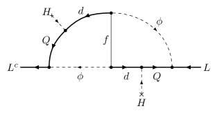
Refer to caption
Figure 1: The neutrino self-energy Feynman diagram. Note that the color-octet fermion f𝑓f is Majorana and therefore we do not add an arrow to the line.

The neutrino self-energy Feynman diagram depicted in Fig. 1 leads to the Majorana neutrino mass matrix

(Mν)ij=4mf(2π)8k,l=13r,s=13α,β=1Nϕ(λikαLQλlαdfVkr)(mdrIrsαβmds)(λjlβLQλkβdfVls),subscriptsubscript𝑀𝜈𝑖𝑗4subscript𝑚𝑓superscript2𝜋8superscriptsubscript𝑘𝑙13superscriptsubscript𝑟𝑠13superscriptsubscript𝛼𝛽1subscript𝑁italic-ϕsuperscriptsubscript𝜆𝑖𝑘𝛼𝐿𝑄superscriptsubscript𝜆𝑙𝛼𝑑𝑓subscript𝑉𝑘𝑟subscript𝑚subscript𝑑𝑟subscript𝐼𝑟𝑠𝛼𝛽subscript𝑚subscript𝑑𝑠superscriptsubscript𝜆𝑗𝑙𝛽𝐿𝑄superscriptsubscript𝜆𝑘𝛽𝑑𝑓subscript𝑉𝑙𝑠(M_{\nu})_{ij}=4\frac{m_{f}}{(2\pi)^{8}}\sum_{k,l=1}^{3}\sum_{r,s=1}^{3}\sum_{\alpha,\beta=1}^{N_{\phi}}\left(\lambda_{ik\alpha}^{LQ}\lambda_{l\alpha}^{df}V_{kr}\right)\left(m_{d_{r}}I_{rs\alpha\beta}m_{d_{s}}\right)\left(\lambda_{jl\beta}^{LQ}\lambda_{k\beta}^{df}V_{ls}\right)\ , (3.1)

where 4 is a color factor, Nϕsubscript𝑁italic-ϕN_{\phi} is the number of leptoquarks ϕαsubscriptitalic-ϕ𝛼\phi_{\alpha}, the integral Iijαβsubscript𝐼𝑖𝑗𝛼𝛽I_{ij\alpha\beta} is defined as

Iijαβd4pd4q1p2mdi21p2mϕα21q2mdj21q2mϕβ21(pq)2mf2,subscript𝐼𝑖𝑗𝛼𝛽superscript𝑑4𝑝superscript𝑑4𝑞1superscript𝑝2superscriptsubscript𝑚subscript𝑑𝑖21superscript𝑝2superscriptsubscript𝑚subscriptitalic-ϕ𝛼21superscript𝑞2superscriptsubscript𝑚subscript𝑑𝑗21superscript𝑞2superscriptsubscript𝑚subscriptitalic-ϕ𝛽21superscript𝑝𝑞2superscriptsubscript𝑚𝑓2I_{ij\alpha\beta}\equiv\int d^{4}p\int d^{4}q\frac{1}{p^{2}-m_{d_{i}}^{2}}\frac{1}{p^{2}-m_{\phi_{\alpha}}^{2}}\frac{1}{q^{2}-m_{d_{j}}^{2}}\frac{1}{q^{2}-m_{\phi_{\beta}}^{2}}\frac{1}{(p-q)^{2}-m_{f}^{2}}\ , (3.2)

and mdisubscript𝑚subscript𝑑𝑖m_{d_{i}} denote the d𝑑d-, s𝑠s- and b𝑏b-quark masses for i=1,2,3𝑖123i=1,2,3, respectively. Note that this is the exact loop integral, using the full propagators for the massive fermions, with the fermion mass factors in the numerator of Eq. 3.1 arising from the chiral projection operators at the vertices. The matrix Mνsubscript𝑀𝜈M_{\nu} corresponds to the effective term (νL)c¯MννL+ν¯LMν(νL)c¯superscriptsubscript𝜈𝐿𝑐subscript𝑀𝜈subscript𝜈𝐿subscript¯𝜈𝐿subscriptsuperscript𝑀𝜈superscriptsubscript𝜈𝐿𝑐\overline{(\nu_{L})^{c}}M_{\nu}\nu_{L}+\overline{\nu}_{L}M^{*}_{\nu}(\nu_{L})^{c}.

For what follows it will be convenient to rewrite Eq. 3.2 in terms of the dimensionless parameters

rimdi2mf2andtαmϕα2mf2.formulae-sequencesubscript𝑟𝑖superscriptsubscript𝑚subscript𝑑𝑖2superscriptsubscript𝑚𝑓2andsubscript𝑡𝛼superscriptsubscript𝑚subscriptitalic-ϕ𝛼2superscriptsubscript𝑚𝑓2r_{i}\equiv\frac{m_{d_{i}}^{2}}{m_{f}^{2}}\quad\quad\mathrm{and}\quad\quad t_{\alpha}\equiv\frac{m_{\phi_{\alpha}}^{2}}{m_{f}^{2}}\;. (3.3)

Specifically, factoring out mf2superscriptsubscript𝑚𝑓2m_{f}^{2} and rescaling the momenta we have:

Iijαβ=1mf2d4pd4q1p2ri1p2tα1q2rj1q2tβ1(pq)21.subscript𝐼𝑖𝑗𝛼𝛽1superscriptsubscript𝑚𝑓2superscript𝑑4𝑝superscript𝑑4𝑞1superscript𝑝2subscript𝑟𝑖1superscript𝑝2subscript𝑡𝛼1superscript𝑞2subscript𝑟𝑗1superscript𝑞2subscript𝑡𝛽1superscript𝑝𝑞21I_{ij\alpha\beta}=\frac{1}{m_{f}^{2}}\int d^{4}p\int d^{4}q\frac{1}{p^{2}-r_{i}}\frac{1}{p^{2}-t_{\alpha}}\frac{1}{q^{2}-r_{j}}\frac{1}{q^{2}-t_{\beta}}\frac{1}{(p-q)^{2}-1}\ . (3.4)

In App. B we exactly evaluate this integral in general, and in the situation where the quark masses are much smaller than the leptoquark ϕitalic-ϕ\phi and color-octet fermion f𝑓f masses – specifically where ri/j0subscript𝑟𝑖𝑗0r_{i/j}\to 0.

We now make some useful approximations. First, since the quark masses are much smaller than those of the leptoquark ϕitalic-ϕ\phi and color-octet fermion f𝑓f, they may be neglected in the denominator. This is equivalent to treating the internal quark lines in the mass-insertion approximation. As mentioned, this case is evaluated in App. B and is denoted

Iαβlimri/j0Iijαβ=1mf2d4pd4q1p2q21p2tα1q2tβ1(pq)21.subscript𝐼𝛼𝛽subscriptsubscript𝑟𝑖𝑗0subscript𝐼𝑖𝑗𝛼𝛽1superscriptsubscript𝑚𝑓2superscript𝑑4𝑝superscript𝑑4𝑞1superscript𝑝2superscript𝑞21superscript𝑝2subscript𝑡𝛼1superscript𝑞2subscript𝑡𝛽1superscript𝑝𝑞21I_{\alpha\beta}\equiv\lim_{r_{i/j}\to 0}I_{ij\alpha\beta}=\frac{1}{m_{f}^{2}}\int d^{4}p\int d^{4}q\frac{1}{p^{2}q^{2}}\frac{1}{p^{2}-t_{\alpha}}\frac{1}{q^{2}-t_{\beta}}\frac{1}{(p-q)^{2}-1}\ . (3.5)

Also, we only consider the parameter space region where the b𝑏b-quark mass dominates the numerator, so that the d𝑑d- and s𝑠s-quark masses may be put to zero. This requires the Yukawa couplings λLQλdfsuperscript𝜆𝐿𝑄superscript𝜆𝑑𝑓\lambda^{LQ}\lambda^{df} to not be strongly hierarchical in the sense of being able to compensate for the hierarchy in the quark masses. So, the formula for the neutrino mass matrix simplifies to

(Mν)ij4mfmb2Vtb2(2π)8α,β=1Nϕ(λi3αLQλ3αdf)(Iαβ)(λj3βLQλ3βdf).similar-to-or-equalssubscriptsubscript𝑀𝜈𝑖𝑗4subscript𝑚𝑓superscriptsubscript𝑚𝑏2superscriptsubscript𝑉𝑡𝑏2superscript2𝜋8superscriptsubscript𝛼𝛽1subscript𝑁italic-ϕsuperscriptsubscript𝜆𝑖3𝛼𝐿𝑄superscriptsubscript𝜆3𝛼𝑑𝑓subscript𝐼𝛼𝛽superscriptsubscript𝜆𝑗3𝛽𝐿𝑄superscriptsubscript𝜆3𝛽𝑑𝑓(M_{\nu})_{ij}\simeq 4\frac{m_{f}m_{b}^{2}V_{tb}^{2}}{(2\pi)^{8}}\sum_{\alpha,\beta=1}^{N_{\phi}}\left(\lambda_{i3\alpha}^{LQ}\lambda_{3\alpha}^{df}\right)\left(I_{\alpha\beta}\right)\left(\lambda_{j3\beta}^{LQ}\lambda_{3\beta}^{df}\right)\ . (3.6)

Equation 3.6 may be simply re-expressed in matrix notation as

Mνconst.×ΛIΛT,M_{\nu}\simeq{\rm const.}\times\Lambda I\Lambda^{T}\ , (3.7)

where

Λiαλi3αLQλ3αdfandI(Iαβ).formulae-sequencesubscriptΛ𝑖𝛼superscriptsubscript𝜆𝑖3𝛼𝐿𝑄superscriptsubscript𝜆3𝛼𝑑𝑓and𝐼subscript𝐼𝛼𝛽\Lambda_{i\alpha}\equiv\lambda_{i3\alpha}^{LQ}\lambda_{3\alpha}^{df}\quad\quad\mathrm{and}\quad\quad I\equiv\left(I_{\alpha\beta}\right)\;. (3.8)

If there were only one leptoquark flavor, I𝐼I would be just a number and ΛΛ\Lambda a 3×1313\times 1 column vector. The neutrino mass matrix would then be of the form of an outer product of a column vector with its transpose, and hence of rank one. With the d𝑑d- and s𝑠s-quark masses switched back on, the exact neutrino mass matrix of Eq. 3.1 is (in general) rank-three, but the two smallest eigenvalues are generally too small to fit the neutrino oscillation data.444As stated earlier, we do not consider the unnatural possibility of a strong hierarchy in the ΛΛ\Lambda values that just happens to offset mdmsmbmuch-less-thansubscript𝑚𝑑subscript𝑚𝑠much-less-thansubscript𝑚𝑏m_{d}\ll m_{s}\ll m_{b}. The necessity of two sufficiently large neutrino mass eigenvalues therefore requires two leptoquark flavors to exist. In that case the third eigenvalue is extremely small and for all practical purposes can be set to zero. Because we choose to adopt the natural parameter space regime where the bottom-quark mass dominates the neutrino mass-matrix formula, from now on we assume that there are only couplings to the third generation in the flavor basis, with the only mixing coming from the SM down-type Yukawa couplings. For most calculations the CKM induced couplings to the first two generations of down-type quarks can be neglected. Hence, we do not discuss the effects of the CKM mixing except in Sec. 5. Given that the smallest neutrino mass almost vanishes, we know that the largest of the neutrino masses is just the square root of the “atmospheric” squared mass difference, namely about 0.05 eV. The new physics in our model must be sufficiently strong to produce this eigenvalue.

It is convenient to solve Eq. 3.6 for the 3×2323\times 2 matrix ΛΛ\Lambda, which can be easily done through a Casas-Ibarra procedure [45]. One obtains

Λiα=j,k=13β=12(2π)42Vtbmbmf(Vν)ij(M^ν12)jkOkβ(I^12S)βα,subscriptΛ𝑖𝛼superscriptsubscript𝑗𝑘13superscriptsubscript𝛽12superscript2𝜋42subscript𝑉𝑡𝑏subscript𝑚𝑏subscript𝑚𝑓subscriptsubscriptsuperscript𝑉𝜈𝑖𝑗subscriptsuperscriptsubscript^𝑀𝜈12𝑗𝑘subscript𝑂𝑘𝛽subscriptsuperscript^𝐼12𝑆𝛽𝛼\Lambda_{i\alpha}=\sum_{j,k=1}^{3}\sum_{\beta=1}^{2}\frac{(2\pi)^{4}}{2V_{tb}m_{b}\sqrt{m_{f}}}\left(V^{*}_{\nu}\right)_{ij}\left(\hat{M}_{\nu}^{\frac{1}{2}}\right)_{jk}O_{k\beta}\left(\hat{I}^{-\frac{1}{2}}S\right)_{\beta\alpha}\ , (3.9)

where Vνsubscript𝑉𝜈V_{\nu} and S𝑆S diagonalize the neutrino mass matrix,

M^ν=VνTMνVν,subscript^𝑀𝜈subscriptsuperscript𝑉𝑇𝜈subscript𝑀𝜈subscript𝑉𝜈\hat{M}_{\nu}=V^{T}_{\nu}M_{\nu}V_{\nu}\ , (3.10)

and the matrix of integrals I𝐼I,

I^=STIS,^𝐼superscript𝑆𝑇𝐼𝑆\hat{I}=S^{T}IS\ , (3.11)

respectively, with I^^𝐼\hat{I} being a real and positive diagonal matrix. The leptonic mixing or PMNS matrix is defined by VPMNS=VeVνsubscript𝑉𝑃𝑀𝑁𝑆superscriptsubscript𝑉𝑒subscript𝑉𝜈V_{PMNS}=V_{e}^{\dagger}V_{\nu}. In the case of a normal [inverted] mass ordering, the first [third] neutrino is massless, i.e. the (1,1) [(3,3)] element of M^νsubscript^𝑀𝜈\hat{M}_{\nu} vanishes and the 2-3 [1-2] sub-block of the matrix O𝑂O is given by a general complex orthogonal matrix, while the first [third] row of O𝑂O is arbitrary. In order to understand the flavor structure of the neutrino mass matrix as well as the bounds on the leptoquark masses in more detail, we have to study the flavor structure of the matrix of integrals I𝐼I, which demands a hierarchy in ΛΛ\Lambda in order to explain a small hierarchy in the neutrino masses.

3.1 Flavor Structure of the Matrix of Integrals 𝑰𝑰I

The main feature of 𝑰𝑰I we wish to demonstrate here is that the matrix develops a hierarchy in its eigenvalues. We will discuss the case with two leptoquarks in detail and generalize it in the end to an arbitrary number of leptoquarks. This hierarchy emerges for a wide range of values of 𝒕𝟏subscript𝒕1t_{1} and 𝒕𝟐subscript𝒕2t_{2} (where 𝟏11 and 𝟐22 distinguish the two leptoquarks as defined in Eq. (3.3)), however it does not have a uniform origin. Firstly if one of the leptoquarks and the octet fermion are much heavier than the other leptoquark, without loss of generality we can take 𝒕𝟏𝟎bold-→subscript𝒕10t_{1}\to 0 and leave 𝒕𝟐subscript𝒕2t_{2} constant. One can check using the analytic expression in App. B that both 𝑰𝟏𝟏subscript𝑰11I_{11} and 𝑰𝟏𝟐=𝑰𝟐𝟏subscript𝑰12subscript𝑰21I_{12}=I_{21} diverge, the former doing so faster, whilst 𝑰𝟐𝟐subscript𝑰22I_{22} remains constant. Accordingly the matrix 𝑰𝑰I becomes singular and thus a hierarchy develops in its eigenvalues. The origin of the hierarchy in this limit is relatively straightforward. Sending 𝒕𝟏𝟎bold-→subscript𝒕10t_{1}\to 0 is equivalent to sending the corresponding leptoquark mass to the mass of the down-type quark that appears in the same loop. In the limit that the two masses are equal a Landau singularity appears and the amplitude associated with the diagram becomes IR divergent. For definiteness, we give an explicit description assuming that 𝒕𝟏𝒕𝟐much-less-thansubscript𝒕1subscript𝒕2t_{1}\ll t_{2} and therefore 𝑰𝟏𝟏𝑰𝟏𝟐𝑰𝟐𝟐much-greater-thansubscript𝑰11subscript𝑰12much-greater-thansubscript𝑰22I_{11}\gg I_{12}\gg I_{22}:

𝑰𝑰𝟏𝟏(𝟏ϵ.𝟎)𝐰𝐢𝐭𝐡ϵ𝑰𝟏𝟐𝑰𝟏𝟏formulae-sequence𝑰subscript𝑰11matrix1bold-italic-ϵabsent0𝐰𝐢𝐭𝐡bold-italic-ϵsubscript𝑰12subscript𝑰11I\approx I_{11}\begin{pmatrix}1&\epsilon\\ .&0\end{pmatrix}\qquad\mathrm{with}\qquad\epsilon\equiv\frac{I_{12}}{I_{11}} (3.12)

neglecting the small 𝑰𝟐𝟐subscript𝑰22I_{22} and we obtain for the inverse square root of the matrix 𝑰𝑰I,

𝑰𝟏𝟐𝑰^𝟏𝟐𝑺=𝑰𝟏𝟏𝟏𝟐(𝒊𝒊ϵ𝟏ϵ).superscript𝑰12superscriptbold-^𝑰12𝑺superscriptsubscript𝑰1112𝒊𝒊bold-italic-ϵ1bold-italic-ϵI^{-\frac{1}{2}}\equiv\hat{I}^{-\frac{1}{2}}S=I_{11}^{-\frac{1}{2}}\left(\begin{array}[]{cc}-i&\frac{i}{\epsilon}\\ 1&\epsilon\\ \end{array}\right)\ . (3.13)

Through Eq. 3.9, this expression feeds into the determination of the required Yukawa couplings 𝚲𝚲\Lambda. Note that the flavor structure above implies that the mixing from the matrix 𝑰𝑰I is small, so the eventual neutrino mixing is mainly determined by the Yukawa couplings in 𝚲𝚲\Lambda.

At the other end of parameter space, consider the case when 𝒕𝟏𝒕𝟐similar-to-or-equalssubscript𝒕1subscript𝒕2t_{1}\simeq t_{2}. It is easy to check using the analytic expressions in App. B that 𝑰𝜶𝜷subscript𝑰𝜶𝜷I_{\alpha\beta} shows a weak dependence on the leptoquark masses. In particular,

|𝒕𝟏𝒕𝟐𝒕𝟐[𝑰𝟏𝟐𝒕𝟏]𝒕𝟏=𝒕𝟐||𝑰𝟐𝟐|.much-less-thansubscript𝒕1subscript𝒕2subscript𝒕2subscriptdelimited-[]subscript𝑰12subscript𝒕1subscript𝒕1subscript𝒕2subscript𝑰22\left|\frac{t_{1}-t_{2}}{t_{2}}\left[\frac{\partial I_{12}}{\partial t_{1}}\right]_{t_{1}=t_{2}}\right|\ll\left|I_{22}\right|\ . (3.14)

As the integral is symmetric in the leptoquark masses, we can expand 𝑰𝑰I as follows

𝑰𝑰𝟐𝟐(𝟏+𝟐ϵ𝟏+ϵ.𝟏)𝐰𝐢𝐭𝐡ϵ𝒕𝟏𝒕𝟐𝒕𝟐𝑰𝟏𝟐𝒕𝟏|𝒕𝟏=𝒕𝟐𝑰𝟐𝟐.formulae-sequence𝑰subscript𝑰22matrix12bold-italic-ϵ1bold-italic-ϵabsent1𝐰𝐢𝐭𝐡bold-italic-ϵsubscript𝒕1subscript𝒕2subscript𝒕2evaluated-atsubscript𝑰12subscript𝒕1subscript𝒕1subscript𝒕2subscript𝑰22I\approx I_{22}\begin{pmatrix}1+2\epsilon&1+\epsilon\\ .&1\\ \end{pmatrix}\qquad\mathrm{with}\qquad\epsilon\equiv\frac{t_{1}-t_{2}}{t_{2}}\frac{\left.\frac{\partial I_{12}}{\partial t_{1}}\right|_{t_{1}=t_{2}}}{I_{22}}\ . (3.15)

Expanding the ratio of the eigenvalues results in a quadratic hierarchy in ϵbold-italic-ϵ\epsilon, given by ϵ𝟐/𝟒+𝓞(ϵ𝟑)superscriptbold-italic-ϵ24𝓞superscriptbold-italic-ϵ3{\epsilon^{2}}/{4}+\mathcal{O}(\epsilon^{3}). This shows that there is a hierarchy in the matrix 𝑰𝑰I for 𝒕𝟏𝒕𝟐similar-to-or-equalssubscript𝒕1subscript𝒕2t_{1}\simeq t_{2} as well. Using this expansion, we obtain a simple expression for the square root of the matrix 𝑰𝑰I,

𝑰𝟏𝟐𝑰^𝟏𝟐𝑺=𝑰𝟐𝟐𝟏𝟐(𝒊|ϵ|𝒊|ϵ|𝟖𝒊|ϵ|𝒊𝟑𝒊|ϵ|𝟖𝟏𝟐𝟏𝟐(𝟏+|ϵ|))+𝓞(ϵ𝟐).superscript𝑰12superscriptbold-^𝑰12𝑺superscriptsubscript𝑰2212matrix𝒊bold-italic-ϵ𝒊bold-italic-ϵ8𝒊bold-italic-ϵ𝒊3𝒊bold-italic-ϵ812121bold-italic-ϵ𝓞superscriptbold-italic-ϵ2I^{-\frac{1}{2}}\equiv\hat{I}^{-\frac{1}{2}}S=I_{22}^{-\frac{1}{2}}\begin{pmatrix}-\frac{i}{|\epsilon|}-\frac{i\left|\epsilon\right|}{8}&\frac{i}{\left|\epsilon\right|}-i-\frac{3\,i\left|\epsilon\right|}{8}\\ \frac{1}{2}&\frac{1}{2}\left(1+\left|\epsilon\right|\right)\\ \end{pmatrix}+\mathcal{O}(\epsilon^{2})\ . (3.16)

Note that the leading contribution, which sets the scale of the couplings 𝚲𝚲\Lambda, is entirely determined by the first row of 𝑰𝟏𝟐superscript𝑰12I^{-\frac{1}{2}}.

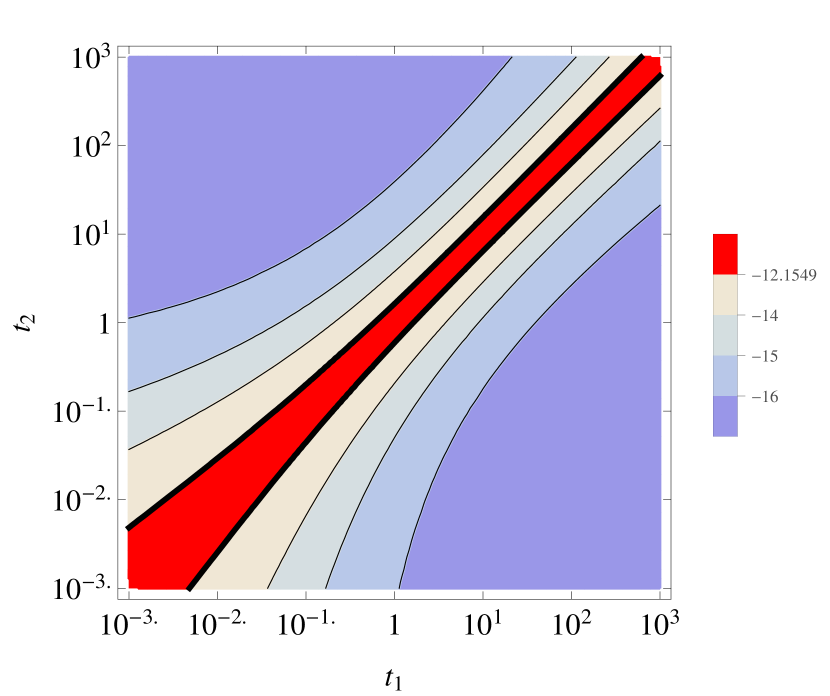
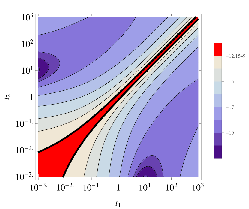
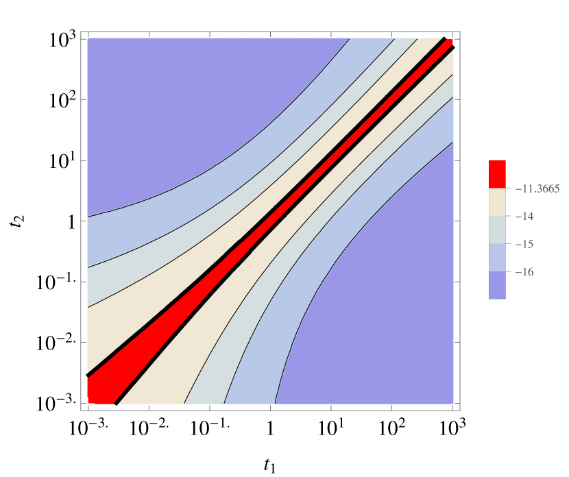
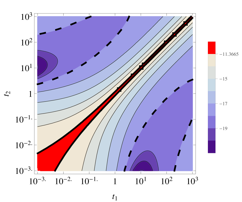
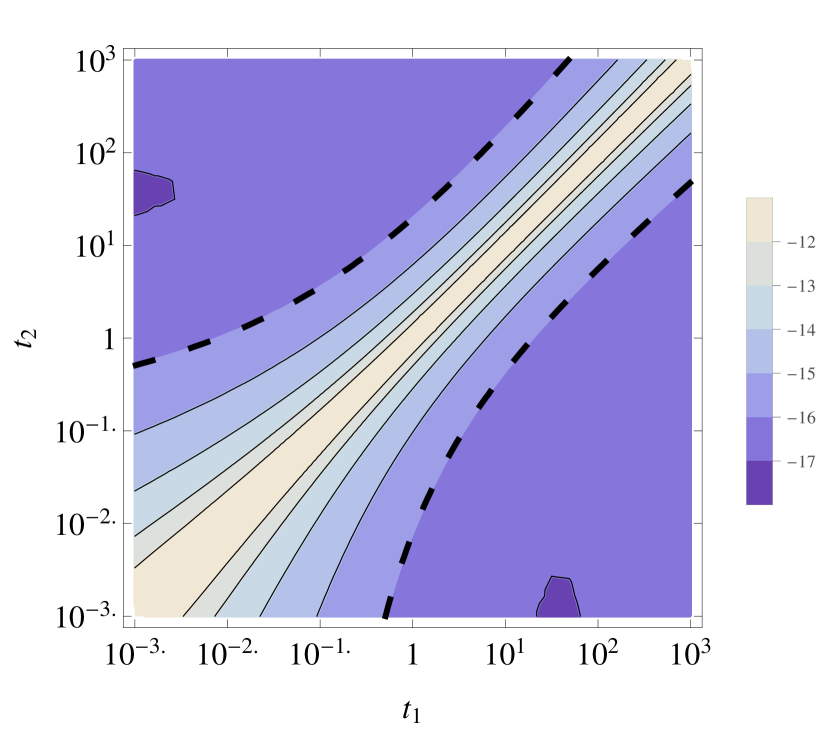
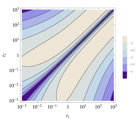
Having understood these two limiting cases, we now draw our attention to the general case, which we analyze numerically. As the absolute mass scale of the integral can be factored out, we see that the hierarchy of the eigenvalues can only depend on the two ratios of masses 𝒕𝜶subscript𝒕𝜶t_{\alpha}. Hence, we show the hierarchy of the eigenvalues in the contour plot in Fig. 2. The mixing angle of the integral matrix is maximal (±𝝅/𝟐plus-or-minus𝝅2\pm\pi/2) for the degenerate case, vanishes for the hierarchical case and can be interpolated between those two limiting cases.
Refer to caption
Figure 2: Contour plot of the hierarchy 𝐥𝐨𝐠𝟏𝟎𝝀𝟏/𝝀𝟐subscript10subscript𝝀1subscript𝝀2\log_{10}\lambda_{1}/\lambda_{2} in the eigenvalues 𝝀𝟏,𝟐subscript𝝀12\lambda_{1,2} of the matrix 𝑰𝑰I as a function of 𝒕𝟏subscript𝒕1t_{1} and 𝒕𝟐subscript𝒕2t_{2} on a logarithmic scale.

The generalization to more generations of leptoquarks is straightforward by grouping the leptoquark masses with a similar mass scale. There is a large hierarchy between the blocks with similar masses due to the mentioned Landau singularity. Additionally, there is a hierarchy between the integrals involving similar leptoquark masses as discussed for the degenerate leptoquark mass case. So if there are three copies of leptoquarks, large hierarchies among the Yukawa couplings 𝚲=𝝀𝑳𝑸𝝀𝒅𝒇𝚲superscript𝝀𝑳𝑸superscript𝝀𝒅𝒇\Lambda=\lambda^{LQ}\lambda^{df} are required to compensate for large hierarchies among the three eigenvalues of the matrix of integral 𝑰𝑰I, which then induces flavor-changing processes that exceed the current limits.

3.2 Understanding the Neutrino Flavor Structure

We can use the approximations from the previous subsection and obtain analytic expressions for the leading order contribution to the neutrino mass matrix.

3.2.1 Normal Mass Ordering

As mentioned above, the 𝟐𝟑232-3 block of the matrix 𝑶𝑶O is given by a complex orthogonal matrix parameterized by the complex angle 𝜽𝜽\theta:

𝑶=(𝐜𝐨𝐬𝜽𝐬𝐢𝐧𝜽𝐬𝐢𝐧𝜽𝐜𝐨𝐬𝜽).𝑶matrix𝜽𝜽𝜽𝜽O=\begin{pmatrix}\cos\theta&-\sin\theta\\ \sin\theta&\cos\theta\\ \end{pmatrix}\ . (3.17)

Consider the expression (𝑴^𝝂𝟏𝟐)𝒋𝒌𝑶𝒌𝜷(𝑰𝟏𝟐)𝜷𝜶subscriptsuperscriptsubscriptbold-^𝑴𝝂12𝒋𝒌subscript𝑶𝒌𝜷subscriptsuperscript𝑰12𝜷𝜶\left(\hat{M}_{\nu}^{\frac{1}{2}}\right)_{jk}O_{k\beta}\left(I^{-\frac{1}{2}}\right)_{\beta\alpha} which appears in Eq. 3.9. In the case of a strong normal hierarchy with 𝒎𝟏=𝟎subscript𝒎10m_{1}=0, the first row vanishes and the resulting leading order approximation to the columns of 𝚲𝚲\Lambda are given by a linear combination of the second and third column of 𝑽𝝂superscriptsubscript𝑽𝝂V_{\nu}^{*}.

We discuss the different limits in turn starting with the strongly hierarchical leptoquark masses, namely 𝒕𝟏𝒕𝟐much-less-thansubscript𝒕1subscript𝒕2t_{1}\ll t_{2}. Here, the leading order contribution is given by

(𝑴^𝝂𝟏𝟐)𝒋𝒌𝑶𝒌𝜷(𝑰𝟏𝟐)𝜷𝜶𝑰𝟏𝟏𝟏𝟐(𝟎𝟎𝒊𝒎𝟐𝒆𝒊𝜽𝒊𝒎𝟐ϵ(𝐜𝐨𝐬𝜽+𝒊ϵ𝟐𝐬𝐢𝐧𝜽)𝒎𝟑𝒆𝒊𝜽𝒎𝟑ϵ(ϵ𝟐𝐜𝐨𝐬𝜽+𝒊𝐬𝐢𝐧𝜽)).similar-to-or-equalssubscriptsuperscriptsubscriptbold-^𝑴𝝂12𝒋𝒌subscript𝑶𝒌𝜷subscriptsuperscript𝑰12𝜷𝜶superscriptsubscript𝑰1112matrix00𝒊subscript𝒎2superscript𝒆𝒊𝜽𝒊subscript𝒎2bold-italic-ϵ𝜽𝒊superscriptbold-italic-ϵ2𝜽subscript𝒎3superscript𝒆𝒊𝜽subscript𝒎3bold-italic-ϵsuperscriptbold-italic-ϵ2𝜽𝒊𝜽\left(\hat{M}_{\nu}^{\frac{1}{2}}\right)_{jk}O_{k\beta}\left(I^{-\frac{1}{2}}\right)_{\beta\alpha}\simeq I_{11}^{-\frac{1}{2}}\begin{pmatrix}0&0\\ -i\sqrt{m_{2}}\,e^{-i\theta}&i\frac{\sqrt{m_{2}}}{\epsilon}\left(\cos\theta+i\epsilon^{2}\sin\theta\right)\\ \sqrt{m_{3}}\,e^{-i\theta}&\frac{\sqrt{m_{3}}}{\epsilon}\left(\epsilon^{2}\cos\theta+i\sin\theta\right)\\ \end{pmatrix}\ . (3.18)

Similarly, in the case of degenerate leptoquark masses, 𝒕𝟏𝒕𝟐similar-to-or-equalssubscript𝒕1subscript𝒕2t_{1}\simeq t_{2}, the leading order contribution results in

(𝑴^𝝂𝟏𝟐)𝒋𝒌𝑶𝒌𝜷(𝑰𝟏𝟐)𝜷𝜶𝑰𝟐𝟐𝟏𝟐(𝟎𝟎𝒊𝒎𝟐𝐜𝐨𝐬𝜽|ϵ|𝒊𝒎𝟐𝐜𝐨𝐬𝜽|ϵ|𝒊𝒎𝟑𝐬𝐢𝐧𝜽|ϵ|𝒊𝒎𝟑𝐬𝐢𝐧𝜽|ϵ|).similar-to-or-equalssubscriptsuperscriptsubscriptbold-^𝑴𝝂12𝒋𝒌subscript𝑶𝒌𝜷subscriptsuperscript𝑰12𝜷𝜶superscriptsubscript𝑰2212matrix00𝒊subscript𝒎2𝜽bold-italic-ϵ𝒊subscript𝒎2𝜽bold-italic-ϵ𝒊subscript𝒎3𝜽bold-italic-ϵ𝒊subscript𝒎3𝜽bold-italic-ϵ\left(\hat{M}_{\nu}^{\frac{1}{2}}\right)_{jk}O_{k\beta}\left(I^{-\frac{1}{2}}\right)_{\beta\alpha}\simeq I_{22}^{-\frac{1}{2}}\begin{pmatrix}0&0\\ -\frac{i\sqrt{m_{2}}\cos\theta}{\left|\epsilon\right|}&\frac{i\sqrt{m_{2}}\cos\theta}{\left|\epsilon\right|}\\ -\frac{i\sqrt{m_{3}}\sin\theta}{\left|\epsilon\right|}&\frac{i\sqrt{m_{3}}\sin\theta}{\left|\epsilon\right|}\\ \end{pmatrix}\ . (3.19)

Note that a non-vanishing mixing angle 𝜽𝜽\theta can lead to substantially larger couplings because 𝒎𝟐𝟐=𝚫𝒎𝟐𝟏𝟐𝚫𝒎𝟑𝟏𝟐=𝒎𝟑𝟐superscriptsubscript𝒎22𝚫superscriptsubscript𝒎212much-less-than𝚫superscriptsubscript𝒎312superscriptsubscript𝒎32m_{2}^{2}=\Delta m_{21}^{2}\ll\Delta m_{31}^{2}=m_{3}^{2}.

3.2.2 Inverted Mass Ordering

In the case of inverted mass ordering, the 𝟏𝟐121-2 block of the matrix 𝑶𝑶O is given by a complex orthogonal matrix. Following the discussion for normal mass ordering, we consider the expression (𝑴^𝝂𝟏𝟐)𝒋𝒌𝑶𝒌𝜷(𝑰𝟏𝟐)𝜷𝜶subscriptsuperscriptsubscriptbold-^𝑴𝝂12𝒋𝒌subscript𝑶𝒌𝜷subscriptsuperscript𝑰12𝜷𝜶\left(\hat{M}_{\nu}^{\frac{1}{2}}\right)_{jk}O_{k\beta}\left(I^{-\frac{1}{2}}\right)_{\beta\alpha}. In the case of a strong inverted hierarchy with 𝒎𝟑=𝟎subscript𝒎30m_{3}=0, the third row vanishes and the resulting leading order approximation to the columns of 𝚲𝚲\Lambda are given by a linear combination of the first and second columns of 𝑽𝝂superscriptsubscript𝑽𝝂V_{\nu}^{*}.

In the limit of a large hierarchy among the leptoquark masses, 𝒕𝟏𝒕𝟐much-less-thansubscript𝒕1subscript𝒕2t_{1}\ll t_{2}, the leading order contribution is given by

(𝑴^𝝂𝟏𝟐)𝒋𝒌𝑶𝒌𝜷(𝑰𝟏𝟐)𝜷𝜶𝑰𝟏𝟏𝟏𝟐(𝒊𝒎𝟏𝒆𝒊𝜽𝒊𝒎𝟏ϵ(𝐜𝐨𝐬𝜽+𝒊ϵ𝟐𝐬𝐢𝐧𝜽)𝒎𝟐𝒆𝒊𝜽𝒎𝟐ϵ(ϵ𝟐𝐜𝐨𝐬𝜽+𝒊𝐬𝐢𝐧𝜽)𝟎𝟎).similar-to-or-equalssubscriptsuperscriptsubscriptbold-^𝑴𝝂12𝒋𝒌subscript𝑶𝒌𝜷subscriptsuperscript𝑰12𝜷𝜶superscriptsubscript𝑰1112matrix𝒊subscript𝒎1superscript𝒆𝒊𝜽𝒊subscript𝒎1bold-italic-ϵ𝜽𝒊superscriptbold-italic-ϵ2𝜽subscript𝒎2superscript𝒆𝒊𝜽subscript𝒎2bold-italic-ϵsuperscriptbold-italic-ϵ2𝜽𝒊𝜽00\left(\hat{M}_{\nu}^{\frac{1}{2}}\right)_{jk}O_{k\beta}\left(I^{-\frac{1}{2}}\right)_{\beta\alpha}\simeq I_{11}^{-\frac{1}{2}}\begin{pmatrix}-i\,\sqrt{m_{1}}\,e^{-i\theta}&\frac{i\sqrt{m_{1}}}{\epsilon}\left(\cos\theta+i\epsilon^{2}\sin\theta\right)\\ \sqrt{m_{2}}\,e^{-i\theta}&\frac{\sqrt{m_{2}}}{\epsilon}\left(\epsilon^{2}\cos\theta+i\sin\theta\right)\\ 0&0\\ \end{pmatrix}\ . (3.20)

In the case of quasi-degenerate leptoquark masses, the expression becomes

(𝑴^𝝂𝟏𝟐)𝒋𝒌𝑶𝒌𝜷(𝑰𝟏𝟐)𝜷𝜶𝑰𝟐𝟐𝟏𝟐(𝒊𝒎𝟏𝐜𝐨𝐬(𝜽)|ϵ|𝒊𝒎𝟏𝐜𝐨𝐬(𝜽)|ϵ|𝒊𝒎𝟐𝐬𝐢𝐧(𝜽)|ϵ|𝒊𝒎𝟐𝐬𝐢𝐧(𝜽)|ϵ|𝟎𝟎).similar-to-or-equalssubscriptsuperscriptsubscriptbold-^𝑴𝝂12𝒋𝒌subscript𝑶𝒌𝜷subscriptsuperscript𝑰12𝜷𝜶superscriptsubscript𝑰2212matrix𝒊subscript𝒎1𝜽bold-italic-ϵ𝒊subscript𝒎1𝜽bold-italic-ϵ𝒊subscript𝒎2𝜽bold-italic-ϵ𝒊subscript𝒎2𝜽bold-italic-ϵ00\left(\hat{M}_{\nu}^{\frac{1}{2}}\right)_{jk}O_{k\beta}\left(I^{-\frac{1}{2}}\right)_{\beta\alpha}\simeq I_{22}^{-\frac{1}{2}}\begin{pmatrix}-\frac{i\sqrt{m_{1}}\cos(\theta)}{\left|\epsilon\right|}&\frac{i\sqrt{m_{1}}\cos(\theta)}{\left|\epsilon\right|}\\ -\frac{i\sqrt{m_{2}}\sin(\theta)}{\left|\epsilon\right|}&\frac{i\sqrt{m_{2}}\sin(\theta)}{\left|\epsilon\right|}\\ 0&0\\ \end{pmatrix}\ . (3.21)

4 Constraints from Flavor Physics Relevant to Neutrino Mass Generation

The Lagrangian in Eq. (2.4) violates the family lepton numbers and the total lepton number explicitly. Thus we expect rare processes, such as 𝝁𝒆𝜸bold-→𝝁𝒆𝜸\mu\to e\gamma, to place limits on the model parameters. Many of these processes proceed through one loop Feynman diagrams and the associated amplitudes can be reduced into Passarino-Veltman integrals [46]. For the convenience of the reader and for future reference, we have compiled our results in Appendix C and made a Mathematica package denoted as ANT publicly available, which is briefly introduced in Sec. 8.

In this section, we restrict ourselves to the contributions which are required by the generation of neutrino mass, i.e. those in Eq. (2.4a). For the coupling 𝝀𝒆𝒖superscript𝝀𝒆𝒖\lambda^{eu} in Eq. (2.4b), which does not enter the neutrino mass formula, we only give an estimation of the constraints in Sec. 5. However, we compiled some of the most relevant full expressions in Appendix A. We extended the FeynRules [47] SM implementation to include the new particles and used FeynArts [48] as well as FormCalc [49] to obtain analytical results for the different processes.

In this work, we fix the mixing angles and mass-squared differences to the experimental best fit values (v1.1) of the NuFIT collaboration [50]555See [51; *Fogli:2012ua] for other global fits to the neutrino oscillation data.

𝐬𝐢𝐧𝟐𝜽𝟏𝟐superscript2subscript𝜽12\displaystyle\sin^{2}\theta_{12} =0.306,absent0.306\displaystyle=0.306\,, 𝚫𝒎𝟐𝟏𝟐𝚫superscriptsubscript𝒎212\displaystyle\Delta m_{21}^{2} =7.45×𝟏𝟎𝟓𝐞𝐕𝟐,absent7.45superscript105superscript𝐞𝐕2\displaystyle=7.45\times 10^{-5}\,\mathrm{eV}^{2}\,,
𝐬𝐢𝐧𝟐𝜽𝟏𝟑superscript2subscript𝜽13\displaystyle\sin^{2}\theta_{13} =0.0231,absent0.0231\displaystyle=0.0231\,, 𝚫𝒎𝟑𝟏𝟐𝚫superscriptsubscript𝒎312\displaystyle\Delta m_{31}^{2} =2.421×𝟏𝟎𝟑𝐞𝐕𝟐(𝑵),absent2.421superscript103superscript𝐞𝐕2𝑵\displaystyle=2.421\times 10^{-3}\,\mathrm{eV}^{2}(N)\,, (4.1)
𝐬𝐢𝐧𝟐𝜽𝟐𝟑superscript2subscript𝜽23\displaystyle\sin^{2}\theta_{23} =0.437,absent0.437\displaystyle=0.437\,, 𝚫𝒎𝟑𝟐𝟐𝚫superscriptsubscript𝒎322\displaystyle\Delta m_{32}^{2} =2.410×𝟏𝟎𝟑𝐞𝐕𝟐(𝑰).absent2.410superscript103superscript𝐞𝐕2𝑰\displaystyle=-2.410\times 10^{-3}\,\mathrm{eV}^{2}(I)\ .

Furthermore we set the lightest neutrino mass to zero and assume vanishing CP phases in the PMNS matrix, i.e. 𝜹=𝝋𝟏=𝝋𝟐=𝟎𝜹subscript𝝋1subscript𝝋20\delta=\varphi_{1}=\varphi_{2}=0 as well as a vanishing mixing in the matrix 𝑶𝑶O in the Casas-Ibarra-type parameterization of the Yukawa couplings 𝚲𝚲\Lambda. We expect stronger bounds for non-vanishing CP phases or non-vanishing mixing in the matrix 𝑶𝑶O. We leave the discussion of non-vanishing CP phases in the PMNS matrix as well as a non-vanishing mixing in 𝑶𝑶O for future work. Currently there are no bounds on the Yukawa couplings 𝝀𝟑𝜶𝒅𝒇subscriptsuperscript𝝀𝒅𝒇3𝜶\lambda^{df}_{3\alpha} and, for simplicity, we will conservatively set them to a rather large value of 𝟏11 in this work. A detailed study would require each 𝝀𝟑𝜶𝒅𝒇subscriptsuperscript𝝀𝒅𝒇3𝜶\lambda^{df}_{3\alpha} to be varied separately. However simple arguments are already enough to understand the qualitative behavior. The neutrino mass quadratically depends on the combination 𝚲𝒊𝜶=𝝀𝒊𝟑𝜶𝑳𝑸𝝀𝟑𝜶𝒅𝒇subscript𝚲𝒊𝜶subscriptsuperscript𝝀𝑳𝑸𝒊3𝜶subscriptsuperscript𝝀𝒅𝒇3𝜶\Lambda_{i\alpha}=\lambda^{LQ}_{i3\alpha}\lambda^{df}_{3\alpha} and thus a change in the coupling 𝝀𝟑𝜶𝒅𝒇subscriptsuperscript𝝀𝒅𝒇3𝜶\lambda^{df}_{3\alpha} by a factor 𝝃𝝃\xi has to be compensated by a factor 𝝃𝟏superscript𝝃1\xi^{-1} in the coupling 𝝀𝒊𝟑𝜶𝑳𝑸subscriptsuperscript𝝀𝑳𝑸𝒊3𝜶\lambda^{LQ}_{i3\alpha} in order to leave the neutrino mass matrix unchanged. The most important flavor-changing processes turn out to be the LFV decays 𝝁𝒆𝜸bold-→𝝁𝒆𝜸\mu\to e\gamma, 𝝁𝒆𝒆𝒆bold-→𝝁𝒆𝒆𝒆\mu\to eee as well as 𝝁𝒆bold-↔𝝁𝒆\mu\leftrightarrow e conversion in nuclei, which all depend on 𝝀𝒊𝟑𝜶𝑳𝑸subscriptsuperscript𝝀𝑳𝑸𝒊3𝜶\lambda^{LQ}_{i3\alpha}. The dominant contributions to the amplitudes of 𝝁𝒆𝒆𝒆bold-→𝝁𝒆𝒆𝒆\mu\to eee and 𝝁𝒆bold-↔𝝁𝒆\mu\leftrightarrow e conversion in nuclei originate from penguin diagrams which are proportional to 𝝀𝟐𝟑𝜶𝑳𝑸𝝀𝟏𝟑𝜶𝑳𝑸subscriptsuperscript𝝀𝑳𝑸23𝜶subscriptsuperscript𝝀𝑳𝑸13𝜶\lambda^{LQ}_{23\alpha}\lambda^{LQ*}_{13\alpha}. Similarly the amplitude of 𝝁𝒆𝜸bold-→𝝁𝒆𝜸\mu\to e\gamma is proportional to 𝝀𝟐𝟑𝜶𝑳𝑸𝝀𝟏𝟑𝜶𝑳𝑸subscriptsuperscript𝝀𝑳𝑸23𝜶subscriptsuperscript𝝀𝑳𝑸13𝜶\lambda^{LQ}_{23\alpha}\lambda^{LQ*}_{13\alpha}. Hence a decrease of 𝝀𝟑𝜶𝒅𝒇subscriptsuperscript𝝀𝒅𝒇3𝜶\lambda^{df}_{3\alpha} by a factor of 𝝃𝝃\xi leads to an enhancement of the relevant branching ratios by a factor of about 𝝃𝟒superscript𝝃4\xi^{-4} and consequently a stronger constraint.

4.1 Radiative Lepton Flavor Violating Decays 𝒍𝒊𝒍𝒋𝜸bold-→superscriptsubscript𝒍𝒊superscriptsubscript𝒍𝒋𝜸l_{i}^{-}\to l_{j}^{-}\gamma

The first constraints considered are those arising from lepton flavor violating (LFV) processes of the form 𝒍𝒊𝒍𝒋𝜸bold-→superscriptsubscript𝒍𝒊superscriptsubscript𝒍𝒋𝜸l_{i}^{-}\to l_{j}^{-}\gamma, such as 𝝁𝒆𝜸bold-→𝝁𝒆𝜸\mu\to e\gamma, which are shown in Fig. 3.

Refer to caption
Figure 3: Lepton-flavor violating rare decays. The photon can be attached to any of the four lines.

From [53] and the Lagrangian in Eq. (2.4), the amplitude for such processes in this model can be written as

𝓜(𝒍𝒊𝒍𝒋𝜸)=𝒆ϵ𝝁𝒖¯(𝒑𝒋)𝒊𝝈𝝁𝝂𝒒𝝂(𝝈𝑳𝒊𝒋𝑷𝑳+𝝈𝑹𝒊𝒋𝑷𝑹)𝒖(𝒑𝒊),𝓜bold-→subscript𝒍𝒊subscript𝒍𝒋𝜸𝒆superscriptsubscriptbold-italic-ϵ𝝁bold-¯𝒖subscript𝒑𝒋𝒊superscript𝝈𝝁𝝂subscript𝒒𝝂subscript𝝈𝑳𝒊𝒋subscript𝑷𝑳subscript𝝈𝑹𝒊𝒋subscript𝑷𝑹𝒖subscript𝒑𝒊\mathcal{M}(l_{i}\to l_{j}\gamma)=e\epsilon_{\mu}^{*}\bar{u}(p_{j})i\sigma^{\mu\nu}q_{\nu}(\sigma_{Lij}P_{L}+\sigma_{Rij}P_{R})u(p_{i})\ , (4.2)

where 𝒆𝒆e is the electric charge, 𝑷𝑳,𝑹𝟏𝟐(𝟏𝜸𝟓)subscript𝑷𝑳𝑹12minus-or-plus1subscript𝜸5P_{L,R}\equiv\frac{1}{2}\left(1\mp\gamma_{5}\right) are the projection operators and the coefficients666The full expressions for σL,Rsubscript𝜎𝐿𝑅\sigma_{L,R} can be found in Appendix A. 𝝈𝑳,𝑹subscript𝝈𝑳𝑹\sigma_{L,R} are given by

𝝈𝑳𝒊𝒋subscript𝝈𝑳𝒊𝒋\displaystyle\sigma_{Lij} =𝒎𝒍𝒋𝟏𝟔𝝅𝟐𝒎=𝟏𝟐𝝀𝒊𝟑𝒎𝑳𝑸𝝀𝒋𝟑𝒎𝑳𝑸𝒎ϕ𝒎𝟐𝑭(𝒕𝟑𝒎),absentsubscript𝒎subscript𝒍𝒋16superscript𝝅2superscriptsubscript𝒎12superscriptsubscript𝝀𝒊3𝒎𝑳𝑸superscriptsubscript𝝀𝒋3𝒎𝑳𝑸bold-†superscriptsubscript𝒎subscriptbold-italic-ϕ𝒎2𝑭subscript𝒕3𝒎\displaystyle=\frac{m_{l_{j}}}{16\pi^{2}}\sum_{m=1}^{2}\frac{\lambda_{i3m}^{LQ}\lambda_{j3m}^{LQ\dagger}}{m_{\phi_{m}}^{2}}F(t_{3m})\ , 𝝈𝑹𝒊𝒋subscript𝝈𝑹𝒊𝒋\displaystyle\sigma_{Rij} =𝒎𝒍𝒊𝟏𝟔𝝅𝟐𝒎=𝟏𝟐𝝀𝒊𝟑𝒎𝑳𝑸𝝀𝒋𝟑𝒎𝑳𝑸𝒎ϕ𝒎𝟐𝑭(𝒕𝟑𝒎),absentsubscript𝒎subscript𝒍𝒊16superscript𝝅2superscriptsubscript𝒎12superscriptsubscript𝝀𝒊3𝒎𝑳𝑸superscriptsubscript𝝀𝒋3𝒎𝑳𝑸bold-†superscriptsubscript𝒎subscriptbold-italic-ϕ𝒎2𝑭subscript𝒕3𝒎\displaystyle=\frac{m_{l_{i}}}{16\pi^{2}}\sum_{m=1}^{2}\frac{\lambda_{i3m}^{LQ}\lambda_{j3m}^{LQ\dagger}}{m_{\phi_{m}}^{2}}F(t_{3m})\ , (4.3)

where the mass ratio 𝒕𝟑𝒎=𝒎𝒕𝟐/𝒎ϕ𝒎𝟐subscript𝒕3𝒎superscriptsubscript𝒎𝒕2superscriptsubscript𝒎subscriptbold-italic-ϕ𝒎2t_{3m}=m_{t}^{2}/m_{\phi_{m}}^{2} and the loop function 𝑭𝑭F is defined as

𝑭(𝒕𝟑𝒎)=𝟏+𝟒𝒕𝟑𝒎𝟓𝒕𝟑𝒎𝟐+𝟐𝒕𝟑𝒎(𝟐+𝒕𝟑𝒎)𝐥𝐧𝒕𝟑𝒎𝟒(𝒕𝟑𝒎𝟏)𝟒.𝑭subscript𝒕3𝒎14subscript𝒕3𝒎5superscriptsubscript𝒕3𝒎22subscript𝒕3𝒎2subscript𝒕3𝒎subscript𝒕3𝒎4superscriptsubscript𝒕3𝒎14F(t_{3m})=\frac{1+4t_{3m}-5t_{3m}^{2}+2t_{3m}(2+t_{3m})\ln t_{3m}}{4(t_{3m}-1)^{4}}\ . (4.4)

Then, the resulting partial decay width of 𝒍𝒊𝒍𝒋𝜸bold-→subscript𝒍𝒊subscript𝒍𝒋𝜸l_{i}\to l_{j}\gamma is

𝚪(𝒍𝒊𝒍𝒋𝜸)=(𝒎𝒍𝒊𝟐𝒎𝒍𝒋𝟐)𝟑𝒆𝟐(|𝝈𝑳|𝟐+|𝝈𝑹|𝟐)𝟏𝟔𝝅𝒎𝒍𝒊𝟑.𝚪bold-→subscript𝒍𝒊subscript𝒍𝒋𝜸superscriptsuperscriptsubscript𝒎subscript𝒍𝒊2superscriptsubscript𝒎subscript𝒍𝒋23superscript𝒆2superscriptsubscript𝝈𝑳2superscriptsubscript𝝈𝑹216𝝅superscriptsubscript𝒎subscript𝒍𝒊3\Gamma(l_{i}\to l_{j}\gamma)=\frac{(m_{l_{i}}^{2}-m_{l_{j}}^{2})^{3}e^{2}\left(|\sigma_{L}|^{2}+|\sigma_{R}|^{2}\right)}{16\pi m_{l_{i}}^{3}}\ . (4.5)

A comparison to the dominant tree-level decay 𝒍𝒊𝒍𝒋𝝂𝒊𝝂¯𝒋bold-→superscriptsubscript𝒍𝒊superscriptsubscript𝒍𝒋subscript𝝂𝒊subscriptbold-¯𝝂𝒋l_{i}^{-}\to l_{j}^{-}\nu_{i}\bar{\nu}_{j}, neglecting the final state lepton mass, results in a good analytic estimate of the branching ratio for 𝝁𝒆𝜸bold-→𝝁𝒆𝜸\mu\to e\gamma,

𝐁𝐫(𝝁𝒆𝜸)𝟑𝒔𝑾𝟐𝟖𝝅𝟑𝜶(𝒎=𝟏𝟐𝝀𝟐𝟑𝒎𝑳𝑸𝝀𝟏𝟑𝒎𝑳𝑸𝒎𝑾𝟐𝒎ϕ𝒎𝟐𝑭(𝒕𝟑𝒎))𝟐similar-to-or-equals𝐁𝐫bold-→𝝁𝒆𝜸3superscriptsubscript𝒔𝑾28superscript𝝅3𝜶superscriptsuperscriptsubscript𝒎12superscriptsubscript𝝀23𝒎𝑳𝑸superscriptsubscript𝝀13𝒎𝑳𝑸bold-†superscriptsubscript𝒎𝑾2superscriptsubscript𝒎subscriptbold-italic-ϕ𝒎2𝑭subscript𝒕3𝒎2\mathrm{Br}(\mu\to e\gamma)\simeq\frac{3s_{W}^{2}}{8\pi^{3}\alpha}\left(\sum_{m=1}^{2}\lambda_{23m}^{LQ}\lambda_{13m}^{LQ\dagger}\frac{m_{W}^{2}}{m_{\phi_{m}}^{2}}\,F(t_{3m})\right)^{2} (4.6)

with 𝒔𝑾𝟐=𝐬𝐢𝐧𝟐𝜽𝑾superscriptsubscript𝒔𝑾2superscript2subscript𝜽𝑾s_{W}^{2}=\sin^{2}\theta_{W}, which captures the main dependence on the leptoquark masses 𝒎ϕ𝒎𝟐superscriptsubscript𝒎subscriptbold-italic-ϕ𝒎2m_{\phi_{m}}^{2} and couplings 𝝀𝒊𝟑𝒎𝑳𝑸subscriptsuperscript𝝀𝑳𝑸𝒊3𝒎\lambda^{LQ}_{i3m}. In the numerical evaluation, we use the full expression of the partial decay width and the experimentally measured total decay width.
Refer to caption
(a) 𝐥𝐨𝐠𝟏𝟎𝐁𝐫(𝝁𝒆𝜸)subscript10𝐁𝐫bold-→𝝁𝒆𝜸\log_{10}\mathrm{Br}(\mu\to e\gamma) for 𝒎𝒇=𝟏𝐓𝐞𝐕subscript𝒎𝒇1𝐓𝐞𝐕m_{f}=1\,\mathrm{TeV}
Refer to caption
(b) 𝐥𝐨𝐠𝟏𝟎𝐁𝐫(𝝁𝒆𝜸)subscript10𝐁𝐫bold-→𝝁𝒆𝜸\log_{10}\mathrm{Br}(\mu\to e\gamma) for 𝒎𝒇=𝟏𝟎𝐓𝐞𝐕subscript𝒎𝒇10𝐓𝐞𝐕m_{f}=10\,\mathrm{TeV}
Refer to caption
(c) 𝐥𝐨𝐠𝟏𝟎𝐁𝐫(𝝉𝒆𝜸)subscript10𝐁𝐫bold-→𝝉𝒆𝜸\log_{10}\mathrm{Br}(\tau\to e\gamma) for 𝒎𝒇=𝟏𝐓𝐞𝐕subscript𝒎𝒇1𝐓𝐞𝐕m_{f}=1\,\mathrm{TeV}
Refer to caption
(d) 𝐥𝐨𝐠𝟏𝟎𝐁𝐫(𝝉𝝁𝜸)subscript10𝐁𝐫bold-→𝝉𝝁𝜸\log_{10}\mathrm{Br}(\tau\to\mu\gamma) for 𝒎𝒇=𝟏𝐓𝐞𝐕subscript𝒎𝒇1𝐓𝐞𝐕m_{f}=1\,\mathrm{TeV}
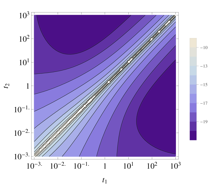
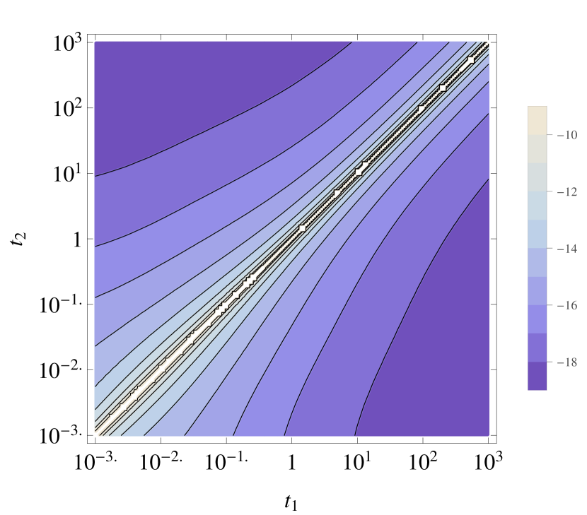
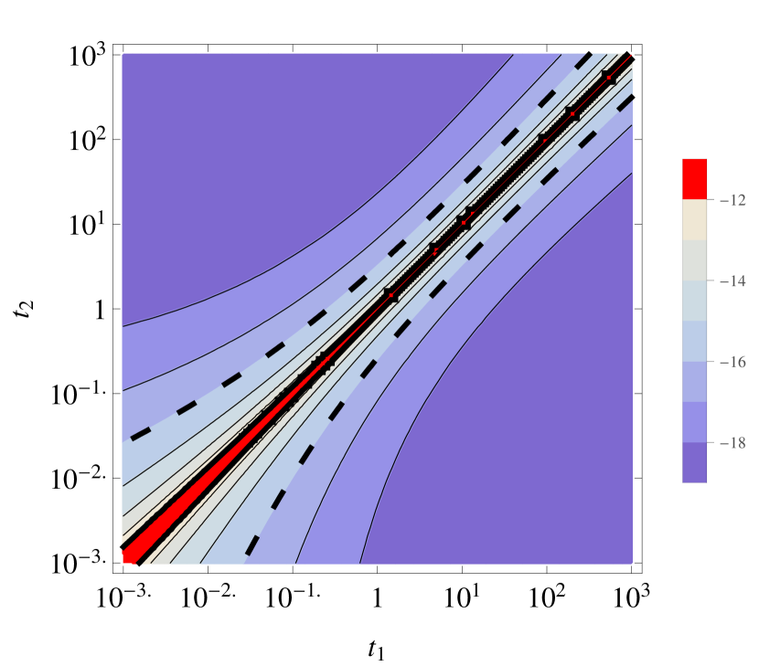
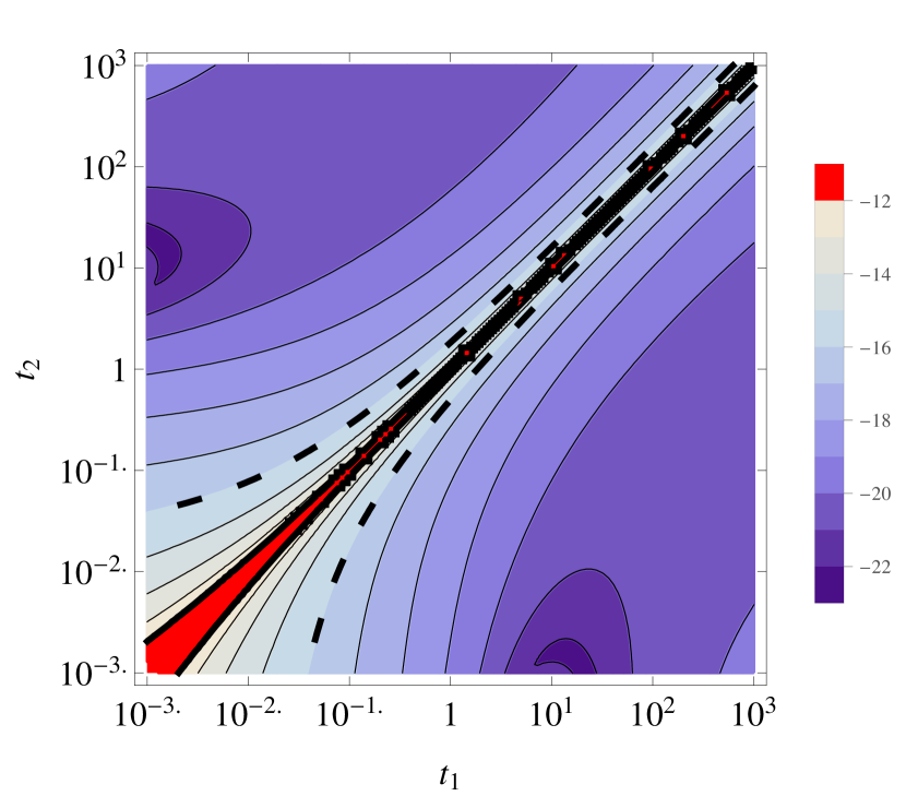
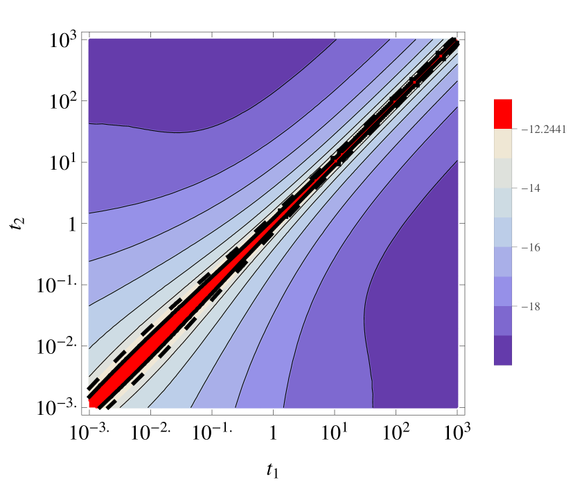
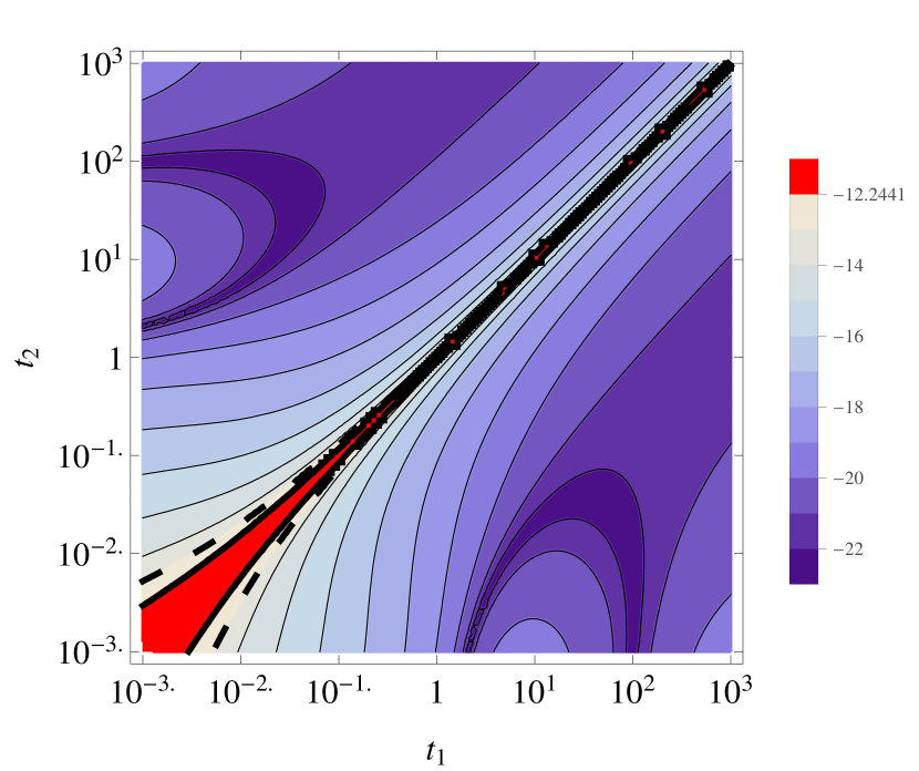
Figure 4: Contour plots of the branching ratio in 𝝁𝒆𝜸bold-→𝝁𝒆𝜸\mu\to e\gamma at 𝒎𝒇=𝟏𝐓𝐞𝐕subscript𝒎𝒇1𝐓𝐞𝐕m_{f}=1\ \,\mathrm{TeV} (top left), 𝒎𝒇=𝟏𝟎𝐓𝐞𝐕subscript𝒎𝒇10𝐓𝐞𝐕m_{f}=10\ \,\mathrm{TeV} (top right), 𝝉𝒆𝜸bold-→𝝉𝒆𝜸\tau\to e\gamma at 𝒎𝒇=𝟏𝐓𝐞𝐕subscript𝒎𝒇1𝐓𝐞𝐕m_{f}=1\ \,\mathrm{TeV} (bottom left) and 𝝉𝝁𝜸bold-→𝝉𝝁𝜸\tau\to\mu\gamma at 𝒎𝒇=𝟏𝐓𝐞𝐕subscript𝒎𝒇1𝐓𝐞𝐕m_{f}=1\ \,\mathrm{TeV} (bottom right). The current exclusion region at Br(𝝁𝒆𝜸)<5.7×𝟏𝟎𝟏𝟑bold-→𝝁𝒆𝜸5.7superscript1013(\mu\to e\gamma)<5.7\times 10^{-13} [54] as well as Br(𝝉𝒆𝜸)<3.3×𝟏𝟎𝟖bold-→𝝉𝒆𝜸3.3superscript108(\tau\to e\gamma)<3.3\times 10^{-8} and Br(𝝉𝝁𝜸)<4.4×𝟏𝟎𝟖bold-→𝝉𝝁𝜸4.4superscript108(\tau\to\mu\gamma)<4.4\times 10^{-8} [55] at 90% C.L. are plotted in red. The sensitivity of the proposed upgrade of MEG is 𝟔×𝟏𝟎𝟏𝟒6superscript10146\times 10^{-14} [56] and it is shown as a dashed black line. The Yukawa couplings 𝝀𝟑𝜶𝒅𝒇subscriptsuperscript𝝀𝒅𝒇3𝜶\lambda^{df}_{3\alpha} are set to 1.

Here we present the contour plots of the branching ratio of 𝝁𝒆𝜸bold-→𝝁𝒆𝜸\mu\to e\gamma at 𝒎𝒇=𝟏𝐓𝐞𝐕subscript𝒎𝒇1𝐓𝐞𝐕m_{f}=1\,\mathrm{TeV} and 𝒎𝒇=𝟏𝟎𝐓𝐞𝐕subscript𝒎𝒇10𝐓𝐞𝐕m_{f}=10\,\mathrm{TeV} in Fig. 4(a) and Fig. 4(b). As expected, the region where 𝒕𝟏𝒕𝟐similar-to-or-equalssubscript𝒕1subscript𝒕2t_{1}\simeq t_{2} is excluded, because the large hierarchy in the integral matrix 𝑰𝑰I needs to be compensated by a large hierarchy in the Yukawa couplings 𝚲𝚲\Lambda, which then leads to a large decay width for 𝝁𝒆𝜸bold-→𝝁𝒆𝜸\mu\to e\gamma. For the same 𝒎𝒇subscript𝒎𝒇m_{f}, the hierarchy gets larger in the third quadrant when leptoquark masses get smaller as shown in Fig. 2, which leads to a wider exclusion region. For the same 𝒕𝟏subscript𝒕1t_{1} and 𝒕𝟐subscript𝒕2t_{2}, the branching ratio in the first quadrant scales as 𝒎𝒇𝟏superscriptsubscript𝒎𝒇1m_{f}^{-1} when 𝒕𝟏𝒕𝟐𝟏similar-to-or-equalssubscript𝒕1subscript𝒕2much-greater-than1t_{1}\simeq t_{2}\gg 1. Thus the exclusion region in the first quadrant is narrower when 𝒎𝒇subscript𝒎𝒇m_{f} gets larger. In the third quadrant where 𝒕𝟏𝒕𝟐𝟏similar-to-or-equalssubscript𝒕1subscript𝒕2much-less-than1t_{1}\simeq t_{2}\ll 1, however, the branching ratio scales as 𝒎𝒇𝟑𝐥𝐧𝒎𝒇𝟐superscriptsubscript𝒎𝒇3superscriptsubscript𝒎𝒇2m_{f}^{3}\ln m_{f}^{2} for fixed 𝒕𝟏subscript𝒕1t_{1} and 𝒕𝟐subscript𝒕2t_{2}. So the exclusion region gets wider when 𝒎𝒇subscript𝒎𝒇m_{f} gets larger. The results for 𝝉𝒆𝜸bold-→𝝉𝒆𝜸\tau\to e\gamma and 𝝉𝝁𝜸bold-→𝝉𝝁𝜸\tau\to\mu\gamma at 𝒎𝒇=𝟏𝐓𝐞𝐕subscript𝒎𝒇1𝐓𝐞𝐕m_{f}=1\,\mathrm{TeV} are shown in Fig. 4(c) and Fig. 4(d) respectively, which are similar but less stringent than the constraints from 𝝁𝒆𝜸bold-→𝝁𝒆𝜸\mu\to e\gamma.

4.2 Anomalous Magnetic Moment

In terms of the functions defined in Eq. (4.3), the anomalous magnetic moment is simply

𝚫𝒂𝒊=𝟐𝒆𝒎𝒍𝒊(𝝈𝑳𝒊𝒊+𝝈𝑹𝒊𝒊)𝒆𝟖𝝅𝟐𝒎=𝟏𝟐|𝝀𝒊𝟑𝒎𝑳𝑸|𝟐𝒎𝒍𝒊𝟐𝒎ϕ𝒎𝟐𝑭(𝒕𝟑𝒎).𝚫subscript𝒂𝒊2𝒆subscript𝒎subscript𝒍𝒊subscript𝝈𝑳𝒊𝒊subscript𝝈𝑹𝒊𝒊similar-to-or-equals𝒆8superscript𝝅2superscriptsubscript𝒎12superscriptsuperscriptsubscript𝝀𝒊3𝒎𝑳𝑸2superscriptsubscript𝒎subscript𝒍𝒊2superscriptsubscript𝒎subscriptbold-italic-ϕ𝒎2𝑭subscript𝒕3𝒎\Delta a_{i}=2\,e\,m_{l_{i}}\,(\sigma_{Lii}+\sigma_{Rii})\simeq\frac{e}{8\pi^{2}}\sum_{m=1}^{2}\left|\lambda_{i3m}^{LQ}\right|^{2}\frac{m_{l_{i}}^{2}}{m_{\phi_{m}}^{2}}F(t_{3m})\ . (4.7)

The predicted values for all three flavors are substantially below current experimental limits, implying that these values do not provide meaningful limits on the model. For example, the maximum contribution to the muon anomalous magnetic moment from our model for 𝒎𝒇=𝟏𝐓𝐞𝐕subscript𝒎𝒇1𝐓𝐞𝐕m_{f}=1\,\mathrm{TeV} is 𝓞(𝟏𝟎𝟏𝟑)𝓞superscript1013\mathcal{O}(10^{-13}), which is almost four orders of magnitude smaller than the experimental uncertainty of 𝚫𝒂𝝁𝒆𝒙𝒑=(1.1659209±0.0000006)×𝟏𝟎𝟑𝚫superscriptsubscript𝒂𝝁𝒆𝒙𝒑plus-or-minus1.16592090.0000006superscript103\Delta a_{\mu}^{exp}=(1.1659209\pm 0.0000006)\times 10^{-3} [55].

4.3 LFV Rare Decay 𝝁𝒆𝒆+𝒆bold-→superscript𝝁superscript𝒆superscript𝒆superscript𝒆\mu^{-}\to e^{-}e^{+}e^{-}

The model has a number of different contributions to 𝝁𝒆𝒆+𝒆bold-→superscript𝝁superscript𝒆superscript𝒆superscript𝒆\mu^{-}\to e^{-}e^{+}e^{-}, including photon penguins, 𝒁𝒁Z-penguins, Higgs penguins and box diagrams. As the Higgs penguin diagrams are suppressed by the electron mass, we have neglected their contribution here. We consider the contribution of the remaining diagrams in turn.777We do not discuss leptonic LFV τ𝜏\tau decays, e.g. τeee𝜏𝑒𝑒𝑒\tau\to eee, since they are less constraining like radiative LFV τ𝜏\tau decays are less constraining than radiative LFV decays of μ𝜇\mu.

To begin with the amplitude associated with the 𝜸𝜸\gamma-penguin can be written as [57; *Hisano:1998fj; *Arganda:2005ji]

𝓜𝜸subscript𝓜𝜸\displaystyle\mathcal{M}_{\gamma} =\displaystyle= 𝒖¯(𝒑𝟏)(𝒒𝟐𝜸𝝁(𝑨𝟏𝑳𝑷𝑳+𝑨𝟏𝑹𝑷𝑹)+𝒊𝒎𝝁𝝈𝝁𝝂𝒒𝝂(𝑨𝟐𝑳𝑷𝑳+𝑨𝟐𝑹𝑷𝑹))𝒖(𝒑)bold-¯𝒖subscript𝒑1superscript𝒒2subscript𝜸𝝁superscriptsubscript𝑨1𝑳subscript𝑷𝑳superscriptsubscript𝑨1𝑹subscript𝑷𝑹𝒊subscript𝒎𝝁subscript𝝈𝝁𝝂superscript𝒒𝝂superscriptsubscript𝑨2𝑳subscript𝑷𝑳superscriptsubscript𝑨2𝑹subscript𝑷𝑹𝒖𝒑\displaystyle\bar{u}(p_{1})\left(q^{2}\gamma_{\mu}(A_{1}^{L}P_{L}+A_{1}^{R}P_{R})+im_{\mu}\sigma_{\mu\nu}q^{\nu}\left(A_{2}^{L}P_{L}+A_{2}^{R}P_{R}\right)\right)u(p) (4.8)
×\displaystyle\times 𝒆𝟐𝒒𝟐𝒖¯(𝒑𝟐)𝜸𝝁𝒗(𝒑𝟑)(𝒑𝟏𝒑𝟐),\displaystyle\frac{e^{2}}{q^{2}}\bar{u}(p_{2})\gamma^{\mu}v(p_{3})-\left(p_{1}\leftrightarrow p_{2}\right)\ ,

where the form factors 𝑨𝟏,𝟐𝑳,𝑹superscriptsubscript𝑨12𝑳𝑹A_{1,2}^{L,R} are given by888The full expressions for A1,2L,Rsuperscriptsubscript𝐴12𝐿𝑅A_{1,2}^{L,R} can be found in Appendix A.

𝑨𝟏𝑳=superscriptsubscript𝑨1𝑳absent\displaystyle A_{1}^{L}= 𝒂=𝟏𝟑𝒎=𝟏𝟐𝝀𝟐𝒂𝒎𝑳𝑸𝝀𝟏𝒂𝒎𝑳𝑸𝟑𝟖𝟒𝝅𝟐𝒎ϕ𝒎𝟐(𝒕𝒂𝒎𝟏)(𝟏𝟎+(𝟏𝟕+𝒕𝒂𝒎)𝒕𝒂𝒎)𝟐(𝟒𝟔𝒕𝒂𝒎𝒕𝒂𝒎𝟑)𝐥𝐧𝒕𝒂𝒎(𝒕𝒂𝒎𝟏)𝟒superscriptsubscript𝒂13superscriptsubscript𝒎12subscriptsuperscript𝝀𝑳𝑸2𝒂𝒎subscriptsuperscript𝝀𝑳𝑸bold-†1𝒂𝒎384superscript𝝅2superscriptsubscript𝒎subscriptbold-italic-ϕ𝒎2subscript𝒕𝒂𝒎11017subscript𝒕𝒂𝒎subscript𝒕𝒂𝒎246subscript𝒕𝒂𝒎superscriptsubscript𝒕𝒂𝒎3subscript𝒕𝒂𝒎superscriptsubscript𝒕𝒂𝒎14\displaystyle\sum_{a=1}^{3}\sum_{m=1}^{2}\frac{\lambda^{LQ}_{2am}\lambda^{LQ\dagger}_{1am}}{384\pi^{2}m_{\phi_{m}}^{2}}\frac{\left(t_{am}-1\right)\left(10+\left(-17+t_{am}\right)t_{am}\right)-2\left(4-6t_{am}-t_{am}^{3}\right)\ln t_{am}}{(t_{am}-1)^{4}} (4.9a)
𝑨𝟏𝑹=superscriptsubscript𝑨1𝑹absent\displaystyle A_{1}^{R}= 𝟎0\displaystyle 0 (4.9b)
𝑨𝟐𝑳,𝑹=superscriptsubscript𝑨2𝑳𝑹absent\displaystyle A_{2}^{L,R}= 𝝈𝑳𝟐𝟏,𝑹𝟐𝟏𝒎𝝁,subscript𝝈𝑳21𝑹21subscript𝒎𝝁\displaystyle\frac{\sigma_{L21,R21}}{m_{\mu}}\ , (4.9c)

where 𝒕𝒂𝒎=𝒎𝒖𝒂𝟐/𝒎ϕ𝒎𝟐subscript𝒕𝒂𝒎superscriptsubscript𝒎subscript𝒖𝒂2superscriptsubscript𝒎subscriptbold-italic-ϕ𝒎2t_{am}=m_{u_{a}}^{2}/m_{\phi_{m}}^{2} and 𝝈𝑳,𝑹subscript𝝈𝑳𝑹\sigma_{L,R} are as defined in Eq. 4.3. Note that the external momentum as well as the electron mass 𝒎𝒆subscript𝒎𝒆m_{e} have been set to zero and all color factors have been taken into account.

Next the contribution from the 𝒁𝒁Z-penguin diagrams can be written as

𝓜𝒁subscript𝓜𝒁\displaystyle\mathcal{M}_{Z} =\displaystyle= 𝟏𝒎𝒁𝟐𝒖¯(𝒑𝟏)𝜸𝝁(𝑭𝑳𝑷𝑳+𝑭𝑹𝑷𝑹)𝒖(𝒑)1superscriptsubscript𝒎𝒁2bold-¯𝒖subscript𝒑1subscript𝜸𝝁subscript𝑭𝑳subscript𝑷𝑳subscript𝑭𝑹subscript𝑷𝑹𝒖𝒑\displaystyle\frac{1}{m_{Z}^{2}}\bar{u}(p_{1})\gamma_{\mu}\left(F_{L}P_{L}+F_{R}P_{R}\right)u(p) (4.10)
×\displaystyle\times 𝒖¯(𝒑𝟐)𝜸𝝁(𝒁𝑳𝑷𝑳+𝒁𝑹𝑷𝑹)𝒗(𝒑𝟑)(𝒑𝟏𝒑𝟐),\displaystyle\bar{u}(p_{2})\gamma^{\mu}\left(Z_{L}P_{L}+Z_{R}P_{R}\right)v(p_{3})-(p_{1}\leftrightarrow p_{2})\ ,

where the form factors 𝑭𝑳,𝑹subscript𝑭𝑳𝑹F_{L,R}999The full expressions for FL,Rsuperscript𝐹𝐿𝑅F^{L,R} can be found in Appendix A. and 𝒁𝑳,𝑹subscript𝒁𝑳𝑹Z_{L,R} are given by

𝑭𝑳subscript𝑭𝑳\displaystyle F_{L} =\displaystyle= 𝒂=𝟏𝟑𝒎=𝟏𝟐𝟑𝒆𝝀𝟐𝒂𝒎𝑳𝑸𝝀𝟏𝒂𝒎𝑳𝑸𝟑𝟐𝝅𝟑𝐬𝐢𝐧𝜽𝑾𝐜𝐨𝐬𝜽𝑾𝒕𝒂𝒎(𝟏𝒕𝒂𝒎+𝐥𝐧𝒕𝒂𝒎)(𝒕𝒂𝒎𝟏)𝟐superscriptsubscript𝒂13superscriptsubscript𝒎123𝒆subscriptsuperscript𝝀𝑳𝑸2𝒂𝒎subscriptsuperscript𝝀𝑳𝑸bold-†1𝒂𝒎32superscript𝝅3subscript𝜽𝑾subscript𝜽𝑾subscript𝒕𝒂𝒎1subscript𝒕𝒂𝒎subscript𝒕𝒂𝒎superscriptsubscript𝒕𝒂𝒎12\displaystyle\sum_{a=1}^{3}\sum_{m=1}^{2}-\frac{3e\lambda^{LQ}_{2am}\lambda^{LQ\dagger}_{1am}}{32\pi^{3}\sin\theta_{W}\cos\theta_{W}}\frac{t_{am}(1-t_{am}+\ln t_{am})}{(t_{am}-1)^{2}} (4.11a)
𝑭𝑹subscript𝑭𝑹\displaystyle F_{R} =\displaystyle= 𝟎0\displaystyle 0 (4.11b)
𝒁𝑳subscript𝒁𝑳\displaystyle Z_{L} =\displaystyle= 𝒆𝐬𝐢𝐧𝜽𝑾𝐜𝐨𝐬𝜽𝑾(𝟏𝟐+𝐬𝐢𝐧𝜽𝑾𝟐)𝒆subscript𝜽𝑾subscript𝜽𝑾12superscriptsubscript𝜽𝑾2\displaystyle-\frac{e}{\sin\theta_{W}\cos\theta_{W}}\left(-\frac{1}{2}+\sin\theta_{W}^{2}\right) (4.11c)
𝒁𝑹subscript𝒁𝑹\displaystyle Z_{R} =\displaystyle= 𝒆𝐬𝐢𝐧𝜽𝑾𝐜𝐨𝐬𝜽𝑾𝐬𝐢𝐧𝜽𝑾𝟐.𝒆subscript𝜽𝑾subscript𝜽𝑾superscriptsubscript𝜽𝑾2\displaystyle-\frac{e}{\sin\theta_{W}\cos\theta_{W}}\sin\theta_{W}^{2}\ . (4.11d)

Finally for the amplitude of the contribution from box diagrams we have

𝓜𝑩𝒐𝒙subscript𝓜𝑩𝒐𝒙\displaystyle\mathcal{M}_{Box} =\displaystyle= 𝒆𝟐𝑩𝟏𝑳[𝒖¯𝒊(𝒑𝟏)(𝜸𝝁𝑷𝑳)𝒖𝒋(𝒑)][𝒖¯𝒊(𝒑𝟐)(𝜸𝝁𝑷𝑳)𝒗𝒊(𝒑𝟑)]superscript𝒆2superscriptsubscript𝑩1𝑳delimited-[]subscriptbold-¯𝒖𝒊subscript𝒑1superscript𝜸𝝁subscript𝑷𝑳subscript𝒖𝒋𝒑delimited-[]subscriptbold-¯𝒖𝒊subscript𝒑2subscript𝜸𝝁subscript𝑷𝑳subscript𝒗𝒊subscript𝒑3\displaystyle e^{2}B_{1}^{L}\left[\bar{u}_{i}(p_{1})\left(\gamma^{\mu}P_{L}\right)u_{j}(p)\right]\left[\bar{u}_{i}(p_{2})\left(\gamma_{\mu}P_{L}\right)v_{i}(p_{3})\right] (4.12)
+\displaystyle+ 𝒆𝟐𝑩𝟏𝑹[𝒖¯𝒊(𝒑𝟏)(𝜸𝝁𝑷𝑹)𝒖𝒋(𝒑)][𝒖¯𝒊(𝒑𝟐)(𝜸𝝁𝑷𝑹)𝒗𝒊(𝒑𝟑)]superscript𝒆2superscriptsubscript𝑩1𝑹delimited-[]subscriptbold-¯𝒖𝒊subscript𝒑1superscript𝜸𝝁subscript𝑷𝑹subscript𝒖𝒋𝒑delimited-[]subscriptbold-¯𝒖𝒊subscript𝒑2subscript𝜸𝝁subscript𝑷𝑹subscript𝒗𝒊subscript𝒑3\displaystyle e^{2}B_{1}^{R}\left[\bar{u}_{i}(p_{1})\left(\gamma^{\mu}P_{R}\right)u_{j}(p)\right]\left[\bar{u}_{i}(p_{2})\left(\gamma_{\mu}P_{R}\right)v_{i}(p_{3})\right]
+\displaystyle+ 𝒆𝟐𝑩𝟐𝑳{[𝒖¯𝒊(𝒑𝟏)(𝜸𝝁𝑷𝑳)𝒖𝒋(𝒑)][𝒖¯𝒊(𝒑𝟐)(𝜸𝝁𝑷𝑹)𝒗𝒊(𝒑𝟑)](𝒑𝟏𝒑𝟐)}\displaystyle e^{2}B_{2}^{L}\left\{\left[\bar{u}_{i}(p_{1})\left(\gamma^{\mu}P_{L}\right)u_{j}(p)\right]\left[\bar{u}_{i}(p_{2})\left(\gamma_{\mu}P_{R}\right)v_{i}(p_{3})\right]-(p_{1}\leftrightarrow p_{2})\right\}
+\displaystyle+ 𝒆𝟐𝑩𝟐𝑹{[𝒖¯𝒊(𝒑𝟏)(𝜸𝝁𝑷𝑹)𝒖𝒋(𝒑)][𝒖¯𝒊(𝒑𝟐)(𝜸𝝁𝑷𝑳)𝒗𝒊(𝒑𝟑)](𝒑𝟏𝒑𝟐)}\displaystyle e^{2}B_{2}^{R}\left\{\left[\bar{u}_{i}(p_{1})\left(\gamma^{\mu}P_{R}\right)u_{j}(p)\right]\left[\bar{u}_{i}(p_{2})\left(\gamma_{\mu}P_{L}\right)v_{i}(p_{3})\right]-(p_{1}\leftrightarrow p_{2})\right\}
+\displaystyle+ 𝒆𝟐𝑩𝟑𝑳{[𝒖¯𝒊(𝒑𝟏)𝑷𝑳𝒖𝒋(𝒑)][𝒖¯𝒊(𝒑𝟐)𝑷𝑳𝒗𝒊(𝒑𝟑)](𝒑𝟏𝒑𝟐)}\displaystyle e^{2}B_{3}^{L}\left\{\left[\bar{u}_{i}(p_{1})P_{L}u_{j}(p)\right]\left[\bar{u}_{i}(p_{2})P_{L}v_{i}(p_{3})\right]-(p_{1}\leftrightarrow p_{2})\right\}
+\displaystyle+ 𝒆𝟐𝑩𝟑𝑹{[𝒖¯𝒊(𝒑𝟏)𝑷𝑹𝒖𝒋(𝒑)][𝒖¯𝒊(𝒑𝟐)𝑷𝑹𝒗𝒊(𝒑𝟑)](𝒑𝟏𝒑𝟐)}\displaystyle e^{2}B_{3}^{R}\left\{\left[\bar{u}_{i}(p_{1})P_{R}u_{j}(p)\right]\left[\bar{u}_{i}(p_{2})P_{R}v_{i}(p_{3})\right]-(p_{1}\leftrightarrow p_{2})\right\}
+\displaystyle+ 𝒆𝟐𝑩𝟒𝑳{[𝒖¯𝒊(𝒑𝟏)(𝝈𝝁𝝂𝑷𝑳)𝒖𝒋(𝒑)][𝒖¯𝒊(𝒑𝟐)(𝝈𝝁𝝂𝑷𝑳)𝒗𝒊(𝒑𝟑)](𝒑𝟏𝒑𝟐)}\displaystyle e^{2}B_{4}^{L}\left\{\left[\bar{u}_{i}(p_{1})\left(\sigma_{\mu\nu}P_{L}\right)u_{j}(p)\right]\left[\bar{u}_{i}(p_{2})\left(\sigma^{\mu\nu}P_{L}\right)v_{i}(p_{3})\right]-(p_{1}\leftrightarrow p_{2})\right\}
+\displaystyle+ 𝒆𝟐𝑩𝟒𝑹{[𝒖¯𝒊(𝒑𝟏)(𝝈𝝁𝝂𝑷𝑹𝒖𝒋(𝒑))][𝒖¯𝒊(𝒑𝟐)(𝝈𝝁𝝂𝑷𝑹)𝒗𝒊(𝒑𝟑)](𝒑𝟏𝒑𝟐)},\displaystyle e^{2}B_{4}^{R}\left\{\left[\bar{u}_{i}(p_{1})\left(\sigma_{\mu\nu}P_{R}u_{j}(p)\right)\right]\left[\bar{u}_{i}(p_{2})\left(\sigma^{\mu\nu}P_{R}\right)v_{i}(p_{3})\right]-(p_{1}\leftrightarrow p_{2})\right\}\ ,

where the form factors 𝑩𝒊subscript𝑩𝒊B_{i} are given by101010The full expressions for Bisubscript𝐵𝑖B_{i} are given in Appendix A.

𝑩𝟏𝑳superscriptsubscript𝑩1𝑳\displaystyle B_{1}^{L} =\displaystyle= 𝒊,𝒋,𝒎,𝒏𝟑𝟏𝟔𝝅𝟐𝒆𝟐𝝀𝟐𝒊𝒎𝑳𝑸𝝀𝟏𝒊𝒏𝑳𝑸𝝀𝟏𝒋𝒎𝑳𝑸𝝀𝟏𝒋𝒏𝑳𝑸𝑫𝟎𝟎[𝒎ϕ𝒎𝟐,𝒎ϕ𝒏𝟐,𝒎𝒖𝒊𝟐,𝒎𝒖𝒋𝟐],subscript𝒊𝒋𝒎𝒏316superscript𝝅2superscript𝒆2subscriptsuperscript𝝀𝑳𝑸2𝒊𝒎subscriptsuperscript𝝀𝑳𝑸bold-†1𝒊𝒏subscriptsuperscript𝝀𝑳𝑸bold-†1𝒋𝒎subscriptsuperscript𝝀𝑳𝑸1𝒋𝒏subscript𝑫00superscriptsubscript𝒎subscriptbold-italic-ϕ𝒎2superscriptsubscript𝒎subscriptbold-italic-ϕ𝒏2superscriptsubscript𝒎subscript𝒖𝒊2superscriptsubscript𝒎subscript𝒖𝒋2\displaystyle\sum_{i,j,m,n}-\frac{3}{16\pi^{2}e^{2}}\lambda^{LQ}_{2im}\lambda^{LQ\dagger}_{1in}\lambda^{LQ\dagger}_{1jm}\lambda^{LQ}_{1jn}D_{00}\left[m_{\phi_{m}}^{2},m_{\phi_{n}}^{2},m_{u_{i}}^{2},m_{u_{j}}^{2}\right]\ , (4.13a)
𝑩𝟏𝑹=𝑩𝟐,𝟑,𝟒𝑳,𝑹superscriptsubscript𝑩1𝑹superscriptsubscript𝑩234𝑳𝑹\displaystyle B_{1}^{R}=B_{2,3,4}^{L,R} =\displaystyle= 𝟎,0\displaystyle 0, (4.13b)

where 𝟑33 is the color factor and all the external momenta and masses have been neglected. The function 𝑫𝟎𝟎subscript𝑫00D_{00} can be found in App. C. Using the form factors given above, we can write the decay width for 𝝁𝒆𝒆+𝒆bold-→superscript𝝁superscript𝒆superscript𝒆superscript𝒆\mu^{-}\to e^{-}e^{+}e^{-} as follows [59]:

𝚪(𝝁𝒆𝒆+𝒆)=𝚪bold-→superscript𝝁superscript𝒆superscript𝒆superscript𝒆absent\displaystyle\Gamma(\mu^{-}\to e^{-}e^{+}e^{-})= 𝒆𝟒𝟓𝟏𝟐𝝅𝟑𝒎𝝁𝟓[|𝑨𝟏𝑳|𝟐+|𝑨𝟏𝑹|𝟐𝟐(𝑨𝟏𝑳𝑨𝟐𝑹+𝑨𝟐𝑳𝑨𝟏𝑹+𝐡.𝐜.)\displaystyle\frac{e^{4}}{512\pi^{3}}m_{\mu}^{5}\Bigg{[}\left|A_{1}^{L}\right|^{2}+\left|A_{1}^{R}\right|^{2}-2\left(A_{1}^{L}A_{2}^{R*}+A_{2}^{L}A_{1}^{R*}+\mathrm{h.c.}\right) (4.14)
+(|𝑨𝟐𝑳|𝟐+|𝑨𝟐𝑹|𝟐)(𝟏𝟔𝟑𝐥𝐧𝒎𝝁𝒎𝒆𝟐𝟐𝟑)superscriptsuperscriptsubscript𝑨2𝑳2superscriptsuperscriptsubscript𝑨2𝑹2163subscript𝒎𝝁subscript𝒎𝒆223\displaystyle+\left(\left|A_{2}^{L}\right|^{2}+\left|A_{2}^{R}\right|^{2}\right)\left(\frac{16}{3}\ln\frac{m_{\mu}}{m_{e}}-\frac{22}{3}\right)
+𝟏𝟔(|𝑩𝟏𝑳|𝟐+|𝑩𝟏𝑹|𝟐)+𝟏𝟑(|𝑩𝟐𝑳|𝟐+|𝑩𝟐𝑹|𝟐)16superscriptsuperscriptsubscript𝑩1𝑳2superscriptsuperscriptsubscript𝑩1𝑹213superscriptsuperscriptsubscript𝑩2𝑳2superscriptsuperscriptsubscript𝑩2𝑹2\displaystyle+\frac{1}{6}\left(\left|B_{1}^{L}\right|^{2}+\left|B_{1}^{R}\right|^{2}\right)+\frac{1}{3}\left(\left|B_{2}^{L}\right|^{2}+\left|B_{2}^{R}\right|^{2}\right)
+𝟏𝟐𝟒(|𝑩𝟑𝑳|𝟐+|𝑩𝟑𝑹|𝟐)+𝟔(|𝑩𝟒𝑳|𝟐+|𝑩𝟒𝑹|𝟐)124superscriptsuperscriptsubscript𝑩3𝑳2superscriptsuperscriptsubscript𝑩3𝑹26superscriptsuperscriptsubscript𝑩4𝑳2superscriptsuperscriptsubscript𝑩4𝑹2\displaystyle+\frac{1}{24}\left(\left|B_{3}^{L}\right|^{2}+\left|B_{3}^{R}\right|^{2}\right)+6\left(\left|B_{4}^{L}\right|^{2}+\left|B_{4}^{R}\right|^{2}\right)
𝟏𝟐(𝑩𝟑𝑳𝑩𝟒𝑳+𝑩𝟑𝑹𝑩𝟒𝑹+𝐡.𝐜.)\displaystyle-\frac{1}{2}\left(B_{3}^{L}B_{4}^{L*}+B_{3}^{R}B_{4}^{R*}+\mathrm{h.c.}\right)
+𝟏𝟑(𝑨𝟏𝑳𝑩𝟏𝑳+𝑨𝟏𝑹𝑩𝟏𝑹+𝑨𝟏𝑳𝑩𝟐𝑳+𝑨𝟏𝑹𝑩𝟐𝑹+𝐡.𝐜.)\displaystyle+\frac{1}{3}\left(A_{1}^{L}B_{1}^{L*}+A_{1}^{R}B_{1}^{R*}+A_{1}^{L}B_{2}^{L*}+A_{1}^{R}B_{2}^{R*}+\mathrm{h.c.}\right)
𝟐𝟑(𝑨𝟐𝑹𝑩𝟏𝑳+𝑨𝟐𝑳𝑩𝟏𝑹+𝑨𝟐𝑳𝑩𝟐𝑹+𝑨𝟐𝑹𝑩𝟐𝑳+𝐡.𝐜.)\displaystyle-\frac{2}{3}\left(A_{2}^{R}B_{1}^{L*}+A_{2}^{L}B_{1}^{R*}+A_{2}^{L}B_{2}^{R*}+A_{2}^{R}B_{2}^{L*}+\mathrm{h.c.}\right)
+𝟏𝟑{𝟐(|𝑭𝑳𝑳|𝟐+|𝑭𝑹𝑹|𝟐)+|𝑭𝑳𝑹|𝟐+|𝑭𝑹𝑳|𝟐\displaystyle+\frac{1}{3}\Big{\{}2\left(\left|F_{LL}\right|^{2}+\left|F_{RR}\right|^{2}\right)+\left|F_{LR}\right|^{2}+\left|F_{RL}\right|^{2}
+(𝑩𝟏𝑳𝑭𝑳𝑳+𝑩𝟏𝑹𝑭𝑹𝑹+𝑩𝟐𝑳𝑭𝑳𝑹+𝑩𝟐𝑹𝑭𝑹𝑳+𝐡.𝐜.)\displaystyle+\left(B_{1}^{L}F_{LL}^{*}+B_{1}^{R}F_{RR}^{*}+B_{2}^{L}F_{LR}^{*}+B_{2}^{R}F_{RL}^{*}+\mathrm{h.c.}\right)
+𝟐(𝑨𝟏𝑳𝑭𝑳𝑳+𝑨𝟏𝑹𝑭𝑹𝑹+𝐡.𝐜.)+(𝑨𝟏𝑳𝑭𝑳𝑹+𝑨𝟏𝑹𝑭𝑹𝑳+𝐡.𝐜.)\displaystyle+2\left(A_{1}^{L}F_{LL}^{*}+A_{1}^{R}F_{RR}^{*}+\mathrm{h.c.}\right)+\left(A_{1}^{L}F_{LR}^{*}+A_{1}^{R}F_{RL}^{*}+\mathrm{h.c.}\right)
𝟒(𝑨𝟐𝑹𝑭𝑳𝑳+𝑨𝟐𝑳𝑭𝑹𝑹+𝐡.𝐜.)𝟐(𝑨𝟐𝑳𝑭𝑹𝑳+𝑨𝟐𝑹𝑭𝑳𝑹+𝐡.𝐜.)}],\displaystyle-4\left(A_{2}^{R}F_{LL}^{*}+A_{2}^{L}F_{RR}^{*}+\mathrm{h.c.}\right)-2\left(A_{2}^{L}F_{RL}^{*}+A_{2}^{R}F_{LR}^{*}+\mathrm{h.c.}\right)\Big{\}}\Bigg{]}\ ,

with

𝑭𝑳𝑳subscript𝑭𝑳𝑳\displaystyle F_{LL} =𝑭𝑳𝒁𝑳𝒈𝟐𝒔𝑾𝟐𝒎𝒁𝟐,absentsubscript𝑭𝑳subscript𝒁𝑳superscript𝒈2superscriptsubscript𝒔𝑾2superscriptsubscript𝒎𝒁2\displaystyle=\frac{F_{L}Z_{L}}{g^{2}s_{W}^{2}m_{Z}^{2}}\ , 𝑭𝑹𝑹subscript𝑭𝑹𝑹\displaystyle F_{RR} =𝑭𝑳𝑳|𝑳𝑹,absentevaluated-atsubscript𝑭𝑳𝑳bold-↔𝑳𝑹\displaystyle=\left.F_{LL}\right|_{L\leftrightarrow R}\ , 𝑭𝑳𝑹subscript𝑭𝑳𝑹\displaystyle F_{LR} =𝑭𝑳𝒁𝑹𝒈𝟐𝒔𝑾𝟐𝒎𝒁𝟐,absentsubscript𝑭𝑳subscript𝒁𝑹superscript𝒈2superscriptsubscript𝒔𝑾2superscriptsubscript𝒎𝒁2\displaystyle=\frac{F_{L}Z_{R}}{g^{2}s_{W}^{2}m_{Z}^{2}}\ , 𝑭𝑹𝑳subscript𝑭𝑹𝑳\displaystyle F_{RL} =𝑭𝑳𝑹|𝑳𝑹,absentevaluated-atsubscript𝑭𝑳𝑹bold-↔𝑳𝑹\displaystyle=\left.F_{LR}\right|_{L\leftrightarrow R}\ , (4.15)

and an approximate expression for the branching ratio is obtained by dividing by the decay width of the dominant muon decay 𝝁𝒆𝝂¯𝒆𝝂𝝁bold-→superscript𝝁superscript𝒆subscriptbold-¯𝝂𝒆subscript𝝂𝝁\mu^{-}\to e^{-}\bar{\nu}_{e}\nu_{\mu}, as for the rare radiative LFV decay 𝝁𝒆𝜸bold-→𝝁𝒆𝜸\mu\to e\gamma.

Refer to caption
(a) 𝐥𝐨𝐠𝟏𝟎𝐁𝐫(𝝁𝒆𝒆𝒆)subscript10𝐁𝐫bold-→𝝁𝒆𝒆𝒆\log_{10}\mathrm{Br}(\mu\to eee) for 𝒎𝒇=𝟏𝐓𝐞𝐕subscript𝒎𝒇1𝐓𝐞𝐕m_{f}=1\,\mathrm{TeV}
Refer to caption
(b) 𝐥𝐨𝐠𝟏𝟎𝐁𝐫(𝝁𝒆𝒆𝒆)subscript10𝐁𝐫bold-→𝝁𝒆𝒆𝒆\log_{10}\mathrm{Br}(\mu\to eee) for 𝒎𝒇=𝟏𝟎𝐓𝐞𝐕subscript𝒎𝒇10𝐓𝐞𝐕m_{f}=10\,\mathrm{TeV}
Figure 5: Contour plots of the branching ratio in 𝝁𝒆𝒆+𝒆bold-→superscript𝝁superscript𝒆superscript𝒆superscript𝒆\mu^{-}\to e^{-}e^{+}e^{-} at 𝒎𝒇=𝟏𝐓𝐞𝐕subscript𝒎𝒇1𝐓𝐞𝐕m_{f}=1\ \,\mathrm{TeV} (left) and 𝒎𝒇=𝟏𝟎𝐓𝐞𝐕subscript𝒎𝒇10𝐓𝐞𝐕m_{f}=10\ \,\mathrm{TeV} (right). The current exclusion region at Br(𝝁𝒆𝒆𝒆)<𝟏𝟎𝟏𝟐bold-→𝝁𝒆𝒆𝒆superscript1012(\mu\to eee)<10^{-12} at 90% C.L. [55] is plotted in red. The sensitivity of measuring Br(𝝁𝒆𝒆𝒆)bold-→𝝁𝒆𝒆𝒆(\mu\to eee) down to 𝟏𝟎𝟏𝟔superscript101610^{-16} of a proposed future experiment [60] is shown as a dashed black line. The Yukawa couplings 𝝀𝟑𝜶𝒅𝒇subscriptsuperscript𝝀𝒅𝒇3𝜶\lambda^{df}_{3\alpha} are set to 1.

We show the numerical results in contour plots in Fig. 5, where the experimental exclusion region is plotted in red. When we increase the mass of the colored octet from 𝒎𝒇=𝟏𝐓𝐞𝐕subscript𝒎𝒇1𝐓𝐞𝐕m_{f}=1\,\mathrm{TeV} to 𝒎𝒇=𝟏𝟎𝐓𝐞𝐕subscript𝒎𝒇10𝐓𝐞𝐕m_{f}=10\,\mathrm{TeV}, the exclusion region gets smaller in both the first and the third quadrant, because the branching ratio is dominated by the 𝒁𝒁Z-penguin and 𝜸𝜸\gamma-penguin respectively, which scales as 𝒎𝒇𝟑/𝟐𝐥𝐧𝒎𝒇𝟐superscriptsubscript𝒎𝒇32superscriptsubscript𝒎𝒇2m_{f}^{-3/2}\ln m_{f}^{2} in the first quadrant and 𝒎𝒇𝟑𝐥𝐧𝒎𝒇𝟐superscriptsubscript𝒎𝒇3superscriptsubscript𝒎𝒇2m_{f}^{-3}\ln m_{f}^{2} in the third quadrant. Compared with the constraints from 𝝁𝒆𝜸bold-→𝝁𝒆𝜸\mu\to e\gamma, the ones from 𝝁𝒆𝒆𝒆bold-→𝝁𝒆𝒆𝒆\mu\to eee are more stringent in the first quadrant because of the slower decoupling of the contribution from the 𝒁𝒁Z-penguin, while in the third quadrant they are less stringent.

4.4 𝝁𝒆bold-↔𝝁𝒆\mu\leftrightarrow e Conversion in Nuclei

The effective Lagrangian contributing to 𝝁𝒆bold-↔𝝁𝒆\mu\leftrightarrow e conversion in this model is [61]

𝓛𝐢𝐧𝐭subscript𝓛𝐢𝐧𝐭\displaystyle{\cal L}_{\rm int} =\displaystyle= 𝟏𝟐(𝒎𝝁𝑨𝟐𝑳𝝁¯𝝈𝝁𝝂𝑷𝑳𝒆𝑭𝝁𝝂+𝒎𝝁𝑨𝟐𝑹𝝁¯𝝈𝝁𝝂𝑷𝑹𝒆𝑭𝝁𝝂+𝐡.𝐜.)\displaystyle-\frac{1}{2}\left(m_{\mu}A_{2}^{L}\,\bar{\mu}\,\sigma^{\mu\nu}P_{L}eF_{\mu\nu}+m_{\mu}A_{2}^{R}\,\bar{\mu}\,\sigma^{\mu\nu}P_{R}eF_{\mu\nu}+{\rm h.c.}\right) (4.16)
𝒒=𝒖,𝒅,𝒔[(𝒈𝑳𝑺(𝒒)𝒆¯𝑷𝑹𝝁+𝒈𝑹𝑺(𝒒)𝒆¯𝑷𝑳𝝁)𝒒¯𝒒\displaystyle-\sum_{q=u,d,s}\left[{\rule[-8.53581pt]{0.0pt}{28.45274pt}\ }\right.\left(g_{LS(q)}\bar{e}P_{R}\mu+g_{RS(q)}\bar{e}P_{L}\mu\right)\bar{q}q
+(𝒈𝑳𝑷(𝒒)𝒆¯𝑷𝑹𝝁+𝒈𝑹𝑷(𝒒)𝒆¯𝑷𝑳𝝁)𝒒¯𝜸𝟓𝒒subscript𝒈𝑳𝑷𝒒bold-¯𝒆subscript𝑷𝑹𝝁subscript𝒈𝑹𝑷𝒒bold-¯𝒆subscript𝑷𝑳𝝁bold-¯𝒒subscript𝜸5𝒒\displaystyle\hskip 68.28644pt+\left(g_{LP(q)}\bar{e}P_{R}\mu+g_{RP(q)}\bar{e}P_{L}\mu\right)\bar{q}\gamma_{5}q
+(𝒈𝑳𝑽(𝒒)𝒆¯𝜸𝝁𝑷𝑳𝝁+𝒈𝑹𝑽(𝒒)𝒆¯𝜸𝝁𝑷𝑹𝝁)𝒒¯𝜸𝝁𝒒subscript𝒈𝑳𝑽𝒒bold-¯𝒆superscript𝜸𝝁subscript𝑷𝑳𝝁subscript𝒈𝑹𝑽𝒒bold-¯𝒆superscript𝜸𝝁subscript𝑷𝑹𝝁bold-¯𝒒subscript𝜸𝝁𝒒\displaystyle\hskip 68.28644pt+\left(g_{LV(q)}\bar{e}\gamma^{\mu}P_{L}\mu+g_{RV(q)}\bar{e}\gamma^{\mu}P_{R}\mu\right)\bar{q}\gamma_{\mu}q
+(𝒈𝑳𝑨(𝒒)𝒆¯𝜸𝝁𝑷𝑳𝝁+𝒈𝑹𝑨(𝒒)𝒆¯𝜸𝝁𝑷𝑹𝝁)𝒒¯𝜸𝝁𝜸𝟓𝒒subscript𝒈𝑳𝑨𝒒bold-¯𝒆superscript𝜸𝝁subscript𝑷𝑳𝝁subscript𝒈𝑹𝑨𝒒bold-¯𝒆superscript𝜸𝝁subscript𝑷𝑹𝝁bold-¯𝒒subscript𝜸𝝁subscript𝜸5𝒒\displaystyle\hskip 68.28644pt+\left(g_{LA(q)}\bar{e}\gamma^{\mu}P_{L}\mu+g_{RA(q)}\bar{e}\gamma^{\mu}P_{R}\mu\right)\bar{q}\gamma_{\mu}\gamma_{5}q
+𝟏𝟐(𝒈𝑳𝑻(𝒒)𝒆¯𝝈𝝁𝝂𝑷𝑹𝝁+𝒈𝑹𝑻(𝒒)𝒆¯𝝈𝝁𝝂𝑷𝑳𝝁)𝒒¯𝝈𝝁𝝂𝒒+𝐡.𝐜.].\displaystyle\hskip 68.28644pt+\ \frac{1}{2}\left(g_{LT(q)}\bar{e}\sigma^{\mu\nu}P_{R}\mu+g_{RT(q)}\bar{e}\sigma^{\mu\nu}P_{L}\mu\right)\bar{q}\sigma_{\mu\nu}q+{\rm h.c.}\left.{\rule[-8.53581pt]{0.0pt}{28.45274pt}\ }\right]\ .

At one loop, there are several contributions to 𝝁𝒆bold-↔𝝁𝒆\mu\leftrightarrow e conversion in nuclei. The long-range interaction is determined by the electromagnetic dipole contribution, which is described by the coefficients 𝑨𝟐𝑳,𝑹superscriptsubscript𝑨2𝑳𝑹A_{2}^{L,R} defined in Eq. (4.9c). The remaining interactions are short-range interactions. Taking all SM particles lighter than the W boson massless, there is only a contribution to the Wilson coefficient of (𝒆¯𝜸𝝁𝑷𝑳𝝁)(𝒒¯𝜸𝝁𝒒)bold-¯𝒆superscript𝜸𝝁subscript𝑷𝑳𝝁bold-¯𝒒subscript𝜸𝝁𝒒(\bar{e}\gamma^{\mu}P_{L}\mu)(\bar{q}\gamma_{\mu}q) from box, 𝜸𝜸\gamma- as well as 𝒁𝒁Z-penguins:

𝒈𝑳𝑽(𝒅)𝒃𝒐𝒙=superscriptsubscript𝒈𝑳𝑽𝒅𝒃𝒐𝒙absent\displaystyle g_{LV(d)}^{box}= |𝑽𝒕𝒅|𝟐𝟔𝟒𝝅𝟐{𝟐𝒎,𝒏,𝒊𝝀𝟐𝟑𝒎𝑳𝑸𝝀𝟏𝟑𝒏𝑳𝑸𝝀𝒊𝟑𝒏𝑳𝑸𝝀𝒊𝟑𝒎𝑳𝑸𝑫𝟎𝟎(𝟎,𝒎ϕ𝒎𝟐,𝒎ϕ𝒏𝟐,𝒎𝒕𝟐)\displaystyle\frac{|V_{td}|^{2}}{64\pi^{2}}\Bigg{\{}2\sum_{m,n,i}\lambda^{LQ}_{23m}\lambda^{LQ*}_{13n}\lambda^{LQ}_{i3n}\lambda^{LQ*}_{i3m}D_{00}\left(0,m_{\phi_{m}}^{2},m_{\phi_{n}}^{2},m_{t}^{2}\right) (4.17a)
𝒎𝝀𝟐𝟑𝒎𝑳𝑸𝝀𝟏𝟑𝒎𝑳𝑸[𝒎𝒕𝟐𝒚𝒕𝟐𝑫𝟎(𝒎𝑾𝟐,𝒎ϕ𝒎𝟐,𝒎𝒕𝟐,𝒎𝒕𝟐)+𝒈𝟐(𝑪𝟎(𝒎𝑾𝟐,𝟎,𝒎ϕ𝒎𝟐)\displaystyle-\sum_{m}\lambda_{23m}^{LQ}\lambda_{13m}^{LQ*}\Big{[}m_{t}^{2}y_{t}^{2}D_{0}\left(m_{W}^{2},m_{\phi_{m}}^{2},m_{t}^{2},m_{t}^{2}\right)+g^{2}\Big{(}C_{0}\left(m_{W}^{2},0,m_{\phi_{m}}^{2}\right)
+𝒎𝒕𝟐𝑫𝟎(𝒎𝑾𝟐,𝟎,𝒎ϕ𝒎𝟐,𝒎𝒕𝟐)𝟐(𝑫𝟎𝟎(𝒎𝑾𝟐,𝟎,𝒎ϕ𝒎𝟐,𝒎𝒕𝟐)+𝑫𝟎𝟎(𝒎𝑾𝟐,𝒎ϕ𝒎𝟐,𝒎𝒕𝟐,𝒎𝒕𝟐)))]},\displaystyle+m_{t}^{2}D_{0}\left(m_{W}^{2},0,m_{\phi_{m}}^{2},m_{t}^{2}\right)-2\left(D_{00}\left(m_{W}^{2},0,m_{\phi_{m}}^{2},m_{t}^{2}\right)+D_{00}\left(m_{W}^{2},m_{\phi_{m}}^{2},m_{t}^{2},m_{t}^{2}\right)\right)\Big{)}\Big{]}\Bigg{\}}\ ,
𝒈𝑳𝑽(𝒅)𝜸=superscriptsubscript𝒈𝑳𝑽𝒅𝜸absent\displaystyle g_{LV(d)}^{\gamma}= 𝜶𝟏𝟒𝟒𝝅𝒎𝝀𝟐𝟑𝒎𝑳𝑸𝝀𝟏𝟑𝒎𝑳𝑸𝒎ϕ𝒎𝟐𝒕𝟑𝒎𝟑𝟏𝟖𝒕𝟑𝒎𝟐+𝟐𝟕𝒕𝟑𝒎+𝟐(𝒕𝟑𝒎𝟑+𝟔𝒕𝟑𝒎𝟒)𝐥𝐧(𝒕𝟑𝒎)𝟏𝟎(𝒕𝟑𝒎𝟏)𝟒𝜶144𝝅subscript𝒎subscriptsuperscript𝝀𝑳𝑸23𝒎subscriptsuperscript𝝀𝑳𝑸13𝒎superscriptsubscript𝒎subscriptbold-italic-ϕ𝒎2superscriptsubscript𝒕3𝒎318superscriptsubscript𝒕3𝒎227subscript𝒕3𝒎2superscriptsubscript𝒕3𝒎36subscript𝒕3𝒎4subscript𝒕3𝒎10superscriptsubscript𝒕3𝒎14\displaystyle-\frac{\alpha}{144\pi}\sum_{m}\frac{\lambda^{LQ}_{23m}\lambda^{LQ*}_{13m}}{m_{\phi_{m}}^{2}}\frac{t_{3m}^{3}-18t_{3m}^{2}+27t_{3m}+2\left(t_{3m}^{3}+6t_{3m}-4\right)\ln\left(t_{3m}\right)-10}{\left(t_{3m}-1\right)^{4}}\, (4.17b)
𝒈𝑳𝑽(𝒅)𝒁=superscriptsubscript𝒈𝑳𝑽𝒅𝒁absent\displaystyle g_{LV(d)}^{Z}= 𝒈𝟐(𝟒𝒔𝑾𝟐𝟑)𝟏𝟐𝟖𝝅𝟐𝒎𝑾𝟐𝒎𝝀𝟐𝟑𝒎𝑳𝑸𝝀𝟏𝟑𝒎𝑳𝑸𝒕𝟑𝒎(𝒕𝟑𝒎𝐥𝐧(𝒕𝟑𝒎)𝟏)(𝒕𝟑𝒎𝟏)𝟐,\displaystyle\frac{g^{2}\left(4s_{W}^{2}-3\right)}{128\pi^{2}m_{W}^{2}}\sum_{m}\lambda^{LQ}_{23m}\lambda^{LQ*}_{13m}\frac{t_{3m}\left(t_{3m}-\ln\left(t_{3m}\right)-1\right)}{\left(t_{3m}-1\right){}^{2}}\ , (4.17c)

and

𝒈𝑳𝑽(𝒖)𝒃𝒐𝒙=superscriptsubscript𝒈𝑳𝑽𝒖𝒃𝒐𝒙absent\displaystyle g_{LV(u)}^{box}= 𝟎,0\displaystyle 0\ , 𝒈𝑳𝑽(𝒖)𝜸=superscriptsubscript𝒈𝑳𝑽𝒖𝜸absent\displaystyle g_{LV(u)}^{\gamma}= 𝟐𝒈𝑳𝑽(𝒅),2subscript𝒈𝑳𝑽𝒅\displaystyle-2g_{LV(d)}\ , 𝒈𝑳𝑽(𝒖)𝒁=superscriptsubscript𝒈𝑳𝑽𝒖𝒁absent\displaystyle g_{LV(u)}^{Z}= 𝟖𝒔𝑾𝟐𝟑𝟒𝒔𝑾𝟐𝟑𝒈𝑳𝑽(𝒅)𝒁.8superscriptsubscript𝒔𝑾234superscriptsubscript𝒔𝑾23superscriptsubscript𝒈𝑳𝑽𝒅𝒁\displaystyle-\frac{8s_{W}^{2}-3}{4s_{W}^{2}-3}g_{LV(d)}^{Z}\ . (4.18)

The gluon penguin contribution vanishes due to its color structure. As the coherent conversion process dominates, i.e. the final state of the nucleon is the same as the initial state [61], the vector coupling to the sea quarks vanishes and it is enough to consider

𝒈𝑳𝑽(𝒖)=subscript𝒈𝑳𝑽𝒖absent\displaystyle g_{LV(u)}= 𝒈𝑳𝑽(𝒖)𝒃𝒐𝒙+𝒈𝑳𝑽(𝒖)𝜸+𝒈𝑳𝑽(𝒖)𝒁,superscriptsubscript𝒈𝑳𝑽𝒖𝒃𝒐𝒙superscriptsubscript𝒈𝑳𝑽𝒖𝜸superscriptsubscript𝒈𝑳𝑽𝒖𝒁\displaystyle g_{LV(u)}^{box}+g_{LV(u)}^{\gamma}+g_{LV(u)}^{Z}\ , 𝒈𝑳𝑽(𝒅)=subscript𝒈𝑳𝑽𝒅absent\displaystyle g_{LV(d)}= 𝒈𝑳𝑽(𝒅)𝒃𝒐𝒙+𝒈𝑳𝑽(𝒅)𝜸+𝒈𝑳𝑽(𝒅)𝒁.superscriptsubscript𝒈𝑳𝑽𝒅𝒃𝒐𝒙superscriptsubscript𝒈𝑳𝑽𝒅𝜸superscriptsubscript𝒈𝑳𝑽𝒅𝒁\displaystyle g_{LV(d)}^{box}+g_{LV(d)}^{\gamma}+g_{LV(d)}^{Z}\ . (4.19)

The coefficients of the vector interaction with protons and neutrons are defined by

𝒈~𝑳𝑺,𝑹𝑺(𝒑)subscriptsuperscriptbold-~𝒈𝒑𝑳𝑺𝑹𝑺\displaystyle\tilde{g}^{(p)}_{LS,RS} =𝒒𝑮𝑺(𝒒,𝒑)𝒈𝑳𝑺,𝑹𝑺(𝒒),absentsubscript𝒒superscriptsubscript𝑮𝑺𝒒𝒑subscript𝒈𝑳𝑺𝑹𝑺𝒒\displaystyle=\sum_{q}G_{S}^{(q,p)}g_{LS,RS(q)}\ , 𝒈~𝑳𝑺,𝑹𝑺(𝒏)subscriptsuperscriptbold-~𝒈𝒏𝑳𝑺𝑹𝑺\displaystyle\tilde{g}^{(n)}_{LS,RS} =𝒒𝑮𝑺(𝒒,𝒏)𝒈𝑳𝑺,𝑹𝑺(𝒒),absentsubscript𝒒superscriptsubscript𝑮𝑺𝒒𝒏subscript𝒈𝑳𝑺𝑹𝑺𝒒\displaystyle=\sum_{q}G_{S}^{(q,n)}g_{LS,RS(q)}\ , (4.20)
𝒈~𝑳𝑽(𝒑)superscriptsubscriptbold-~𝒈𝑳𝑽𝒑\displaystyle\tilde{g}_{LV}^{(p)} =𝟐𝒈𝑳𝑽(𝒖)+𝒈𝑳𝑽(𝒅),absent2subscript𝒈𝑳𝑽𝒖subscript𝒈𝑳𝑽𝒅\displaystyle=2\,g_{LV(u)}+g_{LV(d)}\ , 𝒈~𝑳𝑽(𝒏)superscriptsubscriptbold-~𝒈𝑳𝑽𝒏\displaystyle\tilde{g}_{LV}^{(n)} =𝒈𝑳𝑽(𝒖)+𝟐𝒈𝑳𝑽(𝒅),absentsubscript𝒈𝑳𝑽𝒖2subscript𝒈𝑳𝑽𝒅\displaystyle=g_{LV(u)}+2\,g_{LV(d)}\ , (4.21)

with the coefficients 𝑮𝑺(𝒖,𝒑)=𝑮𝑺(𝒅,𝒏)=5.1subscriptsuperscript𝑮𝒖𝒑𝑺subscriptsuperscript𝑮𝒅𝒏𝑺5.1G^{(u,p)}_{S}=G^{(d,n)}_{S}=5.1, 𝑮𝑺(𝒖,𝒏)=𝑮𝑺(𝒅,𝒑)=4.3subscriptsuperscript𝑮𝒖𝒏𝑺subscriptsuperscript𝑮𝒅𝒑𝑺4.3G^{(u,n)}_{S}=G^{(d,p)}_{S}=4.3 and 𝑮𝑺(𝒔,𝒑)=𝑮𝑺(𝒔,𝒏)=2.5subscriptsuperscript𝑮𝒔𝒑𝑺subscriptsuperscript𝑮𝒔𝒏𝑺2.5G^{(s,p)}_{S}=G^{(s,n)}_{S}=2.5 [62; 61].

Refer to caption
(a) 𝐥𝐨𝐠𝟏𝟎𝐁𝐫(𝝁𝐀𝐮𝒆𝐀𝐮)subscript10𝐁𝐫bold-→𝝁𝐀𝐮𝒆𝐀𝐮\log_{10}\mathrm{Br}(\mu\mathrm{Au}\to e\mathrm{Au}) for 𝒎𝒇=𝟏𝐓𝐞𝐕subscript𝒎𝒇1𝐓𝐞𝐕m_{f}=1\,\mathrm{TeV}
Refer to caption
(b) 𝐥𝐨𝐠𝟏𝟎𝐁𝐫(𝝁𝐀𝐮𝒆𝐀𝐮)subscript10𝐁𝐫bold-→𝝁𝐀𝐮𝒆𝐀𝐮\log_{10}\mathrm{Br}(\mu\mathrm{Au}\to e\mathrm{Au}) for 𝒎𝒇=𝟏𝟎𝐓𝐞𝐕subscript𝒎𝒇10𝐓𝐞𝐕m_{f}=10\,\mathrm{TeV}
Refer to caption
(c) 𝐥𝐨𝐠𝟏𝟎𝐁𝐫(𝝁𝐓𝐢𝒆𝐓𝐢)subscript10𝐁𝐫bold-→𝝁𝐓𝐢𝒆𝐓𝐢\log_{10}\mathrm{Br}(\mu\mathrm{Ti}\to e\mathrm{Ti}) for 𝒎𝒇=𝟏𝐓𝐞𝐕subscript𝒎𝒇1𝐓𝐞𝐕m_{f}=1\,\mathrm{TeV}
Refer to caption
(d) 𝐥𝐨𝐠𝟏𝟎𝐁𝐫(𝝁𝐓𝐢𝒆𝐓𝐢)subscript10𝐁𝐫bold-→𝝁𝐓𝐢𝒆𝐓𝐢\log_{10}\mathrm{Br}(\mu\mathrm{Ti}\to e\mathrm{Ti}) for 𝒎𝒇=𝟏𝟎𝐓𝐞𝐕subscript𝒎𝒇10𝐓𝐞𝐕m_{f}=10\,\mathrm{TeV}
Refer to caption
(e) 𝐥𝐨𝐠𝟏𝟎𝐁𝐫(𝝁𝐀𝐥𝒆𝐀𝐥)subscript10𝐁𝐫bold-→𝝁𝐀𝐥𝒆𝐀𝐥\log_{10}\mathrm{Br}(\mu\mathrm{Al}\to e\mathrm{Al}) for 𝒎𝒇=𝟏𝐓𝐞𝐕subscript𝒎𝒇1𝐓𝐞𝐕m_{f}=1\,\mathrm{TeV}
Refer to caption
(f) 𝐥𝐨𝐠𝟏𝟎𝐁𝐫(𝝁𝐀𝐥𝒆𝐀𝐥)subscript10𝐁𝐫bold-→𝝁𝐀𝐥𝒆𝐀𝐥\log_{10}\mathrm{Br}(\mu\mathrm{Al}\to e\mathrm{Al}) for 𝒎𝒇=𝟏𝟎𝐓𝐞𝐕subscript𝒎𝒇10𝐓𝐞𝐕m_{f}=10\,\mathrm{TeV}
Figure 6: Contour plots of the branching ratio of 𝝁𝒆bold-↔𝝁𝒆\mu\leftrightarrow e conversion, current experimental bounds (in red) and prospects (thick dashed lines) in Au𝟕𝟗𝟏𝟗𝟕superscriptsubscriptAu79197{}^{197}_{79}\text{Au} (top), Ti𝟐𝟐𝟒𝟖superscriptsubscriptTi2248{}^{48}_{22}\text{Ti} (center), and Al𝟏𝟑𝟐𝟕superscriptsubscriptAl1327{}^{27}_{13}\text{Al} (bottom) at 𝒎𝒇=𝟏,𝟏𝟎𝐓𝐞𝐕subscript𝒎𝒇110𝐓𝐞𝐕m_{f}=1,10\,\mathrm{TeV}. The Yukawa couplings 𝝀𝟑𝜶𝒅𝒇subscriptsuperscript𝝀𝒅𝒇3𝜶\lambda^{df}_{3\alpha} are set to 1. The current most stringent bound comes from Br(𝝁𝐀𝐮𝒆𝐀𝐮)<𝟕×𝟏𝟎𝟏𝟑bold-→𝝁𝐀𝐮𝒆𝐀𝐮7superscript1013(\mu\mathrm{Au}\to e\mathrm{Au})<7\times 10^{-13} at 90 % C.L. [55] and the best experimental prospects are from Br(𝝁𝐀𝐥𝒆𝐀𝐥)𝟏𝟎𝟏𝟔less-than-or-similar-tobold-→𝝁𝐀𝐥𝒆𝐀𝐥superscript1016(\mu\mathrm{Al}\to e\mathrm{Al})\lesssim 10^{-16} [63; *Cui:2009zz; 65; *Kurup:2011zza; *Kutschke:2011ux] as well as Br(𝝁𝐓𝐢𝒆𝐓𝐢)𝟏𝟎𝟏𝟖less-than-or-similar-tobold-→𝝁𝐓𝐢𝒆𝐓𝐢superscript1018(\mu\mathrm{Ti}\to e\mathrm{Ti})\lesssim 10^{-18} [63; *Cui:2009zz] improving the current limit Br(𝝁𝐓𝐢𝒆𝐓𝐢)<4.3×𝟏𝟎𝟏𝟐bold-→𝝁𝐓𝐢𝒆𝐓𝐢4.3superscript1012(\mu\mathrm{Ti}\to e\mathrm{Ti})<4.3\times 10^{-12} at 90% C.L. [55].

In terms of these expressions, we can express the conversion rate as

𝝎𝐜𝐨𝐧𝐯=subscript𝝎𝐜𝐨𝐧𝐯absent\displaystyle\omega_{\rm conv}= 𝟒|𝟏𝟖𝑨𝟐𝑹𝑫+𝒈~𝑳𝑺(𝒑)𝑺(𝒑)+𝒈~𝑳𝑺(𝒏)𝑺(𝒏)+𝒈~𝑳𝑽(𝒑)𝑽(𝒑)+𝒈~𝑳𝑽(𝒏)𝑽(𝒏)|𝟐4superscript18superscriptsubscript𝑨2𝑹𝑫superscriptsubscriptbold-~𝒈𝑳𝑺𝒑superscript𝑺𝒑superscriptsubscriptbold-~𝒈𝑳𝑺𝒏superscript𝑺𝒏superscriptsubscriptbold-~𝒈𝑳𝑽𝒑superscript𝑽𝒑superscriptsubscriptbold-~𝒈𝑳𝑽𝒏superscript𝑽𝒏2\displaystyle 4\left|\frac{1}{8}A_{2}^{R*}D+\tilde{g}_{LS}^{(p)}S^{(p)}+\tilde{g}_{LS}^{(n)}S^{(n)}+\tilde{g}_{LV}^{(p)}V^{(p)}+\tilde{g}_{LV}^{(n)}V^{(n)}\right|^{2}
+\displaystyle+ 𝟒|𝟏𝟖𝑨𝟐𝑳𝑫+𝒈~𝑹𝑺(𝒑)𝑺(𝒑)+𝒈~𝑹𝑺(𝒏)𝑺(𝒏)+𝒈~𝑹𝑽(𝒑)𝑽(𝒑)+𝒈~𝑹𝑽(𝒏)𝑽(𝒏)|𝟐,4superscript18superscriptsubscript𝑨2𝑳𝑫superscriptsubscriptbold-~𝒈𝑹𝑺𝒑superscript𝑺𝒑superscriptsubscriptbold-~𝒈𝑹𝑺𝒏superscript𝑺𝒏superscriptsubscriptbold-~𝒈𝑹𝑽𝒑superscript𝑽𝒑superscriptsubscriptbold-~𝒈𝑹𝑽𝒏superscript𝑽𝒏2\displaystyle 4\left|\frac{1}{8}A_{2}^{L*}D+\tilde{g}_{RS}^{(p)}S^{(p)}+\tilde{g}_{RS}^{(n)}S^{(n)}+\tilde{g}_{RV}^{(p)}V^{(p)}+\tilde{g}_{RV}^{(n)}V^{(n)}\right|^{2}\ , (4.22)

where the overlap integrals 𝑫𝑫D, 𝑺(𝒑)superscript𝑺𝒑S^{(p)}, 𝑺(𝒏)superscript𝑺𝒏S^{(n)}, 𝑽(𝒑)superscript𝑽𝒑V^{(p)} and 𝑽(𝒏)superscript𝑽𝒏V^{(n)} take values as shown in Tab. 1. The branching ratio is defined by Br(𝝁𝑵𝒆𝑵)𝝎𝒄𝒐𝒏𝒗/𝝎𝒄𝒂𝒑𝒕bold-→𝝁𝑵𝒆𝑵subscript𝝎𝒄𝒐𝒏𝒗subscript𝝎𝒄𝒂𝒑𝒕(\mu N\to eN)\equiv\omega_{conv}/\omega_{capt}.

𝑺(𝒑)superscript𝑺𝒑S^{(p)} 𝑺(𝒏)superscript𝑺𝒏S^{(n)} 𝑽(𝒑)superscript𝑽𝒑V^{(p)} 𝑽(𝒏)superscript𝑽𝒏V^{(n)} 𝑫𝑫D 𝝎𝒄𝒂𝒑𝒕(𝟏𝟎𝟔𝒔𝟏)subscript𝝎𝒄𝒂𝒑𝒕superscript106superscript𝒔1\omega_{capt}(10^{6}s^{-1})
Au𝟕𝟗𝟏𝟗𝟕superscriptsubscriptAu79197{}^{197}_{79}\text{Au} 0.167 0.0523 0.0610 0.0859 0.108 13.07
Ti𝟐𝟐𝟒𝟖superscriptsubscriptTi2248{}^{48}_{22}\text{Ti} 0.0870 0.0371 0.0462 0.0399 0.0495 2.59
Al𝟏𝟑𝟐𝟕superscriptsubscriptAl1327{}^{27}_{13}\text{Al} 0.0169 0.0153 0.0163 0.0357 0.0159 0.7054
Table 1: The overlap integrals in the unit of 𝒎𝝁𝟓/𝟐superscriptsubscript𝒎𝝁52m_{\mu}^{5/2} and the total capture rates for different nuclei. The overlap integrals of Au𝟕𝟗𝟏𝟗𝟕superscriptsubscriptAu79197{}^{197}_{79}\text{Au} as well as Al𝟏𝟑𝟐𝟕superscriptsubscriptAl1327{}^{27}_{13}\text{Al} are taken from Table 2 and Ti𝟐𝟐𝟒𝟖superscriptsubscriptTi2248{}^{48}_{22}\text{Ti} are taken from Table 4 of [61], while the total capture rates are both from Table 8.

In Fig. 6 we present the contour plots of the branching ratio for 𝝁𝒆bold-↔𝝁𝒆\mu\leftrightarrow e conversion in Au𝟕𝟗𝟏𝟗𝟕superscriptsubscriptAu79197{}^{197}_{79}\text{Au}, Ti𝟐𝟐𝟒𝟖superscriptsubscriptTi2248{}^{48}_{22}\text{Ti} and Al𝟏𝟑𝟐𝟕superscriptsubscriptAl1327{}^{27}_{13}\text{Al}, where the first gives the most stringent current constraints and the last two may give the most stringent future ones.111111The bound from μPbePb𝜇Pb𝑒Pb\mu\mathrm{Pb}\to e\mathrm{Pb} conversion by the SINDRUM II experiment [68] is less competitive than μe𝜇𝑒\mu\leftrightarrow e conversion in Au79197superscriptsubscriptAu79197{}^{197}_{79}\text{Au}. The current bounds from 𝝁𝒆bold-↔𝝁𝒆\mu\leftrightarrow e conversion in Au𝟕𝟗𝟏𝟗𝟕superscriptsubscriptAu79197{}^{197}_{79}\text{Au} at 𝒎𝒇=𝟏𝐓𝐞𝐕subscript𝒎𝒇1𝐓𝐞𝐕m_{f}=1\,\mathrm{TeV} and 𝒎𝒇=𝟏𝟎𝐓𝐞𝐕subscript𝒎𝒇10𝐓𝐞𝐕m_{f}=10\,\mathrm{TeV} are plotted in red Fig. 6(a) and Fig. 6(b), which are obviously the most stringent ones so far compared with those from 𝝁𝒆𝜸bold-→𝝁𝒆𝜸\mu\to e\gamma and 𝝁𝒆𝒆𝒆bold-→𝝁𝒆𝒆𝒆\mu\to eee. When we increase the mass of the colored octet, the exclusion region gets smaller because the dominant contribution, the 𝒁𝒁Z-penguin, scales as 𝒎𝒇𝟑/𝟐𝐥𝐧𝒎𝒇𝟐superscriptsubscript𝒎𝒇32superscriptsubscript𝒎𝒇2m_{f}^{-3/2}\ln m_{f}^{2}. For 𝝁𝒆bold-↔𝝁𝒆\mu\leftrightarrow e conversion in Ti𝟐𝟐𝟒𝟖superscriptsubscriptTi2248{}^{48}_{22}\text{Ti}, although the current data gives weaker bounds, the COMET experiment [63; *Cui:2009zz] will be able to explore a much larger region of the parameter space or give the strongest bounds in the future, i.e. the dashed thick line in Fig. 6(d) as well as the whole region shown in Fig. 6(c).

4.5 Other Constraints

In the previous subsection, we discussed the most stringent constraints. In this subsection, we discuss constraints which turn out to be not competitive compared to the constraints from LFV processes. We start with dimension-6 operators generated at tree-level using the list of constraints compiled in Ref. [69], then discuss bounds from meson mixing, the 𝒃𝒔bold-→𝒃𝒔b\to s transition using the constraints in [70; 71] and finally generic dimension-6 operators 𝑳𝑳𝑸𝑸𝑳𝑳𝑸𝑸LLQQ generated at the one-loop order using the list of constraints in Ref. [69].

4.5.1 Processes from 𝚫𝑭=𝟎𝚫𝑭0\Delta F=0 Operators Generated at Tree Level

Integrating out the leptoquarks leads to a few new operators at tree-level involving only the third generation of quarks. In particular, we generate the operators

𝑪𝒊𝒋𝒕𝒕𝒖,𝑳𝑳superscriptsubscript𝑪𝒊𝒋𝒕𝒕bold-ℓ𝒖𝑳𝑳\displaystyle C_{ijtt}^{\ell u,LL} 𝟐𝟐𝑮𝑭(𝒊¯𝜸𝝁𝑷𝑳𝒋)(𝒕¯𝜸𝝁𝑷𝑳𝒕),22subscript𝑮𝑭bold-¯subscriptbold-ℓ𝒊superscript𝜸𝝁subscript𝑷𝑳subscriptbold-ℓ𝒋bold-¯𝒕subscript𝜸𝝁subscript𝑷𝑳𝒕\displaystyle 2\sqrt{2}G_{F}(\bar{\ell_{i}}\gamma^{\mu}P_{L}\ell_{j})(\bar{t}\gamma_{\mu}P_{L}t)\ , 𝑪𝒊𝒋𝒕𝒃𝑪𝑪,𝑳𝑳superscriptsubscript𝑪𝒊𝒋𝒕𝒃𝑪𝑪𝑳𝑳\displaystyle C_{ijtb}^{CC,LL} 𝟐𝟐𝑮𝑭(¯𝒊𝜸𝝁𝑷𝑳𝝂𝒋)(𝒕¯𝜸𝝁𝑷𝑳𝒃),22subscript𝑮𝑭subscriptbold-¯bold-ℓ𝒊superscript𝜸𝝁subscript𝑷𝑳subscript𝝂𝒋bold-¯𝒕subscript𝜸𝝁subscript𝑷𝑳𝒃\displaystyle 2\sqrt{2}G_{F}(\bar{\ell}_{i}\gamma^{\mu}P_{L}\nu_{j})(\bar{t}\gamma_{\mu}P_{L}b)\ , (4.23)
𝑪𝒊𝒋𝒌𝒍𝝂𝒅,𝑳𝑳superscriptsubscript𝑪𝒊𝒋𝒌𝒍𝝂𝒅𝑳𝑳\displaystyle C_{ijkl}^{\nu d,LL} 𝟐𝟐𝑮𝑭(𝝂¯𝒊𝜸𝝁𝑷𝑳𝝂𝒋)(𝒅¯𝒌𝜸𝝁𝑷𝑳𝒅𝒍),22subscript𝑮𝑭subscriptbold-¯𝝂𝒊superscript𝜸𝝁subscript𝑷𝑳subscript𝝂𝒋subscriptbold-¯𝒅𝒌subscript𝜸𝝁subscript𝑷𝑳subscript𝒅𝒍\displaystyle 2\sqrt{2}G_{F}(\bar{\nu}_{i}\gamma^{\mu}P_{L}\nu_{j})(\bar{d}_{k}\gamma_{\mu}P_{L}d_{l})\ , 𝑪𝒊𝒋𝒌𝒍𝝂𝒅,𝑹𝑳superscriptsubscript𝑪𝒊𝒋𝒌𝒍𝝂𝒅𝑹𝑳\displaystyle C_{ijkl}^{\nu d,RL} 𝟐𝟐𝑮𝑭(𝝂¯𝒊𝑪𝜸𝝁𝑷𝑹𝝂𝒋𝑪)(𝒅¯𝒌𝜸𝝁𝑷𝑳𝒅𝒍),22subscript𝑮𝑭superscriptsubscriptbold-¯𝝂𝒊𝑪superscript𝜸𝝁subscript𝑷𝑹superscriptsubscript𝝂𝒋𝑪subscriptbold-¯𝒅𝒌subscript𝜸𝝁subscript𝑷𝑳subscript𝒅𝒍\displaystyle 2\sqrt{2}G_{F}(\bar{\nu}_{i}^{C}\gamma^{\mu}P_{R}\nu_{j}^{C})(\bar{d}_{k}\gamma_{\mu}P_{L}d_{l})\ ,

with their Wilson coefficients given by

𝑪𝒊𝒋𝒕𝒕𝒖,𝑳𝑳superscriptsubscript𝑪𝒊𝒋𝒕𝒕bold-ℓ𝒖𝑳𝑳\displaystyle C_{ijtt}^{\ell u,LL} =𝒎𝝀𝒊𝟑𝒎𝑳𝑸𝝀𝒋𝟑𝒎𝑳𝑸𝟒𝟐𝑮𝑭𝒎ϕ𝒎𝟐,absentsubscript𝒎subscriptsuperscript𝝀𝑳𝑸𝒊3𝒎subscriptsuperscript𝝀𝑳𝑸𝒋3𝒎42subscript𝑮𝑭superscriptsubscript𝒎subscriptbold-italic-ϕ𝒎2\displaystyle=-\sum_{m}\frac{\lambda^{LQ}_{i3m}\lambda^{LQ*}_{j3m}}{4\sqrt{2}G_{F}\,m_{\phi_{m}}^{2}}\ , 𝑪𝒊𝒋𝒕𝒃𝑪𝑪,𝑳𝑳superscriptsubscript𝑪𝒊𝒋𝒕𝒃𝑪𝑪𝑳𝑳\displaystyle C_{ijtb}^{CC,LL} =𝑽𝒕𝒃𝒎𝝀𝒋𝟑𝒎𝑳𝑸𝝀𝒊𝟑𝒎𝑳𝑸𝟒𝟐𝑮𝑭𝒎ϕ𝒎𝟐,absentsubscript𝑽𝒕𝒃subscript𝒎subscriptsuperscript𝝀𝑳𝑸𝒋3𝒎subscriptsuperscript𝝀𝑳𝑸𝒊3𝒎42subscript𝑮𝑭superscriptsubscript𝒎subscriptbold-italic-ϕ𝒎2\displaystyle=V_{tb}\sum_{m}\frac{\lambda^{LQ}_{j3m}\lambda^{LQ*}_{i3m}}{4\sqrt{2}G_{F}\,m_{\phi_{m}}^{2}}\ , (4.24)
𝑪𝒊𝒋𝒌𝒍𝝂𝒅,𝑳𝑳superscriptsubscript𝑪𝒊𝒋𝒌𝒍𝝂𝒅𝑳𝑳\displaystyle C_{ijkl}^{\nu d,LL} =𝑽𝒕𝒌𝑽𝒕𝒍𝒎𝝀𝒋𝟑𝒎𝑳𝑸𝝀𝒊𝟑𝒎𝑳𝑸𝟒𝟐𝑮𝑭𝒎ϕ𝒎𝟐,absentsuperscriptsubscript𝑽𝒕𝒌subscript𝑽𝒕𝒍subscript𝒎subscriptsuperscript𝝀𝑳𝑸𝒋3𝒎subscriptsuperscript𝝀𝑳𝑸𝒊3𝒎42subscript𝑮𝑭superscriptsubscript𝒎subscriptbold-italic-ϕ𝒎2\displaystyle=-V_{tk}^{*}V_{tl}\sum_{m}\frac{\lambda^{LQ*}_{j3m}\lambda^{LQ}_{i3m}}{4\sqrt{2}G_{F}\,m_{\phi_{m}}^{2}}\ , 𝑪𝒊𝒋𝒌𝒍𝝂𝒅,𝑹𝑳superscriptsubscript𝑪𝒊𝒋𝒌𝒍𝝂𝒅𝑹𝑳\displaystyle C_{ijkl}^{\nu d,RL} =𝑽𝒕𝒌𝑽𝒕𝒍𝒎𝝀𝒋𝟑𝒎𝑳𝑸𝝀𝒊𝟑𝒎𝑳𝑸𝟒𝟐𝑮𝑭𝒎ϕ𝒎𝟐.absentsuperscriptsubscript𝑽𝒕𝒌subscript𝑽𝒕𝒍subscript𝒎subscriptsuperscript𝝀𝑳𝑸𝒋3𝒎subscriptsuperscript𝝀𝑳𝑸𝒊3𝒎42subscript𝑮𝑭superscriptsubscript𝒎subscriptbold-italic-ϕ𝒎2\displaystyle=V_{tk}^{*}V_{tl}\sum_{m}\frac{\lambda^{LQ*}_{j3m}\lambda^{LQ}_{i3m}}{4\sqrt{2}G_{F}\,m_{\phi_{m}}^{2}}\ .

There are already weak constraints on the Wilson coefficient 𝑪𝒊𝒋𝒕𝒕𝒖,𝑳𝑳superscriptsubscript𝑪𝒊𝒋𝒕𝒕bold-ℓ𝒖𝑳𝑳C_{ijtt}^{\ell u,LL}, mainly from 𝒁𝒁Z-decay [69]. The most stringent constraint is 𝑪𝝁𝝁𝒕𝒕𝒖,𝑳𝑳<0.061superscriptsubscript𝑪𝝁𝝁𝒕𝒕bold-ℓ𝒖𝑳𝑳0.061C_{\mu\mu tt}^{\ell u,LL}<0.061 from 𝒁𝝁𝝁¯bold-→𝒁𝝁bold-¯𝝁Z\to\mu\bar{\mu}. It translates into

𝒎ϕ𝒎(𝝀𝟐𝟑𝒎𝑳𝑸𝝀𝟐𝟑𝒎𝑳𝑸0.1)×𝟓𝟎𝐆𝐞𝐕greater-than-or-equivalent-tosubscript𝒎subscriptbold-italic-ϕ𝒎subscriptsuperscript𝝀𝑳𝑸23𝒎subscriptsuperscript𝝀𝑳𝑸23𝒎0.150𝐆𝐞𝐕m_{\phi_{m}}\gtrsim\left(\frac{\sqrt{\lambda^{LQ}_{23m}\lambda^{LQ*}_{23m}}}{0.1}\right)\times 50\,\mathrm{GeV} (4.25)

and currently does not pose any competitive constraint. The bound on 𝑪𝒊𝒋𝒕𝒕𝒖,𝑳𝑳superscriptsubscript𝑪𝒊𝒋𝒕𝒕bold-ℓ𝒖𝑳𝑳C_{ijtt}^{\ell u,LL} with 𝒊,𝒋=𝒆,𝝁formulae-sequence𝒊𝒋𝒆𝝁i,j=e,\mu could be improved by measuring the top pair-production cross section at a lepton collider precisely, like a future linear collider. The Wilson coefficient 𝑪𝒊𝒋𝒕𝒃𝑪𝑪,𝑳𝑳superscriptsubscript𝑪𝒊𝒋𝒕𝒃𝑪𝑪𝑳𝑳C_{ijtb}^{CC,LL}, leads to an additional contribution to top decay. We can estimate its relative contribution to the dominant top decay, 𝒕𝑾+𝒃𝒊+𝝂𝒃bold-→𝒕superscript𝑾𝒃bold-→superscriptsubscriptbold-ℓ𝒊𝝂𝒃t\to W^{+}b\to\ell_{i}^{+}\nu b, as

𝒍,𝒎𝑪𝒊𝒋𝒕𝒃𝑪𝑪,𝑳𝑳𝑽𝒕𝒃=𝒋,𝒎𝝀𝒊𝟑𝒎𝑳𝑸𝝀𝒋𝟑𝒎𝑳𝑸𝟒𝟐𝑮𝑭𝒎ϕ𝒎𝟐.subscript𝒍𝒎superscriptsubscript𝑪𝒊𝒋𝒕𝒃𝑪𝑪𝑳𝑳subscript𝑽𝒕𝒃subscript𝒋𝒎superscriptsubscript𝝀𝒊3𝒎𝑳𝑸superscriptsubscript𝝀𝒋3𝒎𝑳𝑸42subscript𝑮𝑭superscriptsubscript𝒎subscriptbold-italic-ϕ𝒎2\sum_{l,m}\frac{C_{ijtb}^{CC,LL}}{V_{tb}}=\sum_{j,m}\frac{\lambda_{i3m}^{LQ*}\lambda_{j3m}^{LQ}}{4\sqrt{2}G_{F}\,m_{\phi_{m}}^{2}}\ . (4.26)

However, the resulting constraint is not as stringent as the constraints from LFV processes. It would require a big improvement of the precision or a dedicated analysis of the angular distribution due to the different angular dependence compared to 𝒕𝑾𝒃bold-→𝒕𝑾𝒃t\to Wb. The Wilson coefficients 𝑪𝒊𝒋𝒃𝒃𝝂𝒃,𝑳𝑳(𝑹𝑳)superscriptsubscript𝑪𝒊𝒋𝒃𝒃𝝂𝒃𝑳𝑳𝑹𝑳C_{ijbb}^{\nu b,LL(RL)} contribute to the invisible decay of 𝚼(𝒏𝑺)𝚼𝒏𝑺\Upsilon(nS) competing with the SM decay mediated by an 𝒔𝒔s-channel 𝒁𝒁Z-boson, but there are no limits and the experimental sensitivity is not good enough to measure even the SM decay. The bounds from semi-leptonic meson decays collected in Tab. 12 in [69] lead to a lower bound on 𝒎ϕ𝒎/𝝀𝒊𝟑𝒎𝑳𝑸𝝀𝒋𝟑𝒎𝑳𝑸subscript𝒎subscriptbold-italic-ϕ𝒎subscriptsuperscript𝝀𝑳𝑸𝒊3𝒎subscriptsuperscript𝝀𝑳𝑸𝒋3𝒎m_{\phi_{m}}/\sqrt{\lambda^{LQ*}_{i3m}\lambda^{LQ}_{j3m}} of the order of 𝟕𝟕𝟎𝐆𝐞𝐕770𝐆𝐞𝐕770\,\mathrm{GeV} for 𝑪𝒊𝒋𝒅𝒔𝝂𝒃,𝑳𝑳(𝑹𝑳)superscriptsubscript𝑪𝒊𝒋𝒅𝒔𝝂𝒃𝑳𝑳𝑹𝑳C_{ijds}^{\nu b,LL(RL)}, 𝟓𝟐𝐆𝐞𝐕52𝐆𝐞𝐕52\,\mathrm{GeV} for 𝑪𝒊𝒋𝒃𝒅𝝂𝒃,𝑳𝑳(𝑹𝑳)superscriptsubscript𝑪𝒊𝒋𝒃𝒅𝝂𝒃𝑳𝑳𝑹𝑳C_{ijbd}^{\nu b,LL(RL)}, 𝟖𝟎𝟎𝐆𝐞𝐕800𝐆𝐞𝐕800\,\mathrm{GeV} for 𝑪𝒊𝒋𝒃𝒔𝝂𝒃,𝑳𝑳(𝑹𝑳)superscriptsubscript𝑪𝒊𝒋𝒃𝒔𝝂𝒃𝑳𝑳𝑹𝑳C_{ijbs}^{\nu b,LL(RL)}. A comparison with realistic values, 𝒎ϕ𝒎𝟏𝟎𝟎𝐆𝐞𝐕greater-than-or-equivalent-tosubscript𝒎subscriptbold-italic-ϕ𝒎100𝐆𝐞𝐕m_{\phi_{m}}\gtrsim 100\,\mathrm{GeV} and |𝝀𝒊𝟑𝒎𝑳𝑸|0.1less-than-or-similar-tosubscriptsuperscript𝝀𝑳𝑸𝒊3𝒎0.1|\lambda^{LQ}_{i3m}|\lesssim 0.1, demonstrates that there is currently no competitive constraint from this class of operators.

4.5.2 Meson Mixing

The most general effective Hamiltonian has the form, following the notation of [72],

𝓗𝐞𝐟𝐟𝒊𝒋=𝒎=𝟏𝟓𝑪𝒎𝒊𝒋𝑸𝒎𝒊𝒋+𝒎=𝟏𝟑𝑪~𝒎𝒊𝒋𝑸~𝒎𝒊𝒋,superscriptsubscript𝓗𝐞𝐟𝐟𝒊𝒋superscriptsubscript𝒎15superscriptsubscript𝑪𝒎𝒊𝒋superscriptsubscript𝑸𝒎𝒊𝒋superscriptsubscript𝒎13superscriptsubscriptbold-~𝑪𝒎𝒊𝒋superscriptsubscriptbold-~𝑸𝒎𝒊𝒋\mathcal{H}_{\rm eff}^{ij}=\sum_{m=1}^{5}C_{m}^{ij}Q_{m}^{ij}+\sum_{m=1}^{3}\tilde{C}_{m}^{ij}\tilde{Q}_{m}^{ij}\ , (4.27)

where the superscripts 𝒊,𝒋𝒊𝒋i,j denote the quark flavors, 𝑪𝒎𝒊𝒋superscriptsubscript𝑪𝒎𝒊𝒋C_{m}^{ij} (𝑪~𝒎𝒊𝒋superscriptsubscriptbold-~𝑪𝒎𝒊𝒋\tilde{C}_{m}^{ij}) the Wilson coefficients and 𝑸𝒎𝒊𝒋superscriptsubscript𝑸𝒎𝒊𝒋Q_{m}^{ij} (𝑸~𝒎𝒊𝒋superscriptsubscriptbold-~𝑸𝒎𝒊𝒋\tilde{Q}_{m}^{ij}) the following operators

𝑸𝟏𝒊𝒋superscriptsubscript𝑸1𝒊𝒋\displaystyle Q_{1}^{ij} =(𝒒¯𝒊𝜶𝜸𝝁𝑷𝑳𝒒𝒋𝜶)(𝒒¯𝒊𝜷𝜸𝝁𝑷𝑳𝒒𝒋𝜷),absentsuperscriptsubscriptbold-¯𝒒𝒊𝜶subscript𝜸𝝁subscript𝑷𝑳superscriptsubscript𝒒𝒋𝜶superscriptsubscriptbold-¯𝒒𝒊𝜷superscript𝜸𝝁subscript𝑷𝑳superscriptsubscript𝒒𝒋𝜷\displaystyle=(\bar{q}_{i}^{\alpha}\gamma_{\mu}P_{L}q_{j}^{\alpha})(\bar{q}_{i}^{\beta}\gamma^{\mu}P_{L}q_{j}^{\beta})\ , 𝑸𝟐𝒊𝒋superscriptsubscript𝑸2𝒊𝒋\displaystyle Q_{2}^{ij} =(𝒒¯𝒊𝜶𝑷𝑳𝒒𝒋𝜶)(𝒒¯𝒊𝜷𝑷𝑳𝒒𝒋𝜷),absentsuperscriptsubscriptbold-¯𝒒𝒊𝜶subscript𝑷𝑳superscriptsubscript𝒒𝒋𝜶superscriptsubscriptbold-¯𝒒𝒊𝜷subscript𝑷𝑳superscriptsubscript𝒒𝒋𝜷\displaystyle=(\bar{q}_{i}^{\alpha}P_{L}q_{j}^{\alpha})(\bar{q}_{i}^{\beta}P_{L}q_{j}^{\beta})\ , 𝑸𝟑𝒊𝒋superscriptsubscript𝑸3𝒊𝒋\displaystyle Q_{3}^{ij} =(𝒒¯𝒊𝜶𝑷𝑳𝒒𝒋𝜷)(𝒒¯𝒊𝜷𝑷𝑳𝒒𝒋𝜶),absentsuperscriptsubscriptbold-¯𝒒𝒊𝜶subscript𝑷𝑳superscriptsubscript𝒒𝒋𝜷superscriptsubscriptbold-¯𝒒𝒊𝜷subscript𝑷𝑳superscriptsubscript𝒒𝒋𝜶\displaystyle=(\bar{q}_{i}^{\alpha}P_{L}q_{j}^{\beta})(\bar{q}_{i}^{\beta}P_{L}q_{j}^{\alpha})\ , (4.28)
𝑸𝟒𝒊𝒋superscriptsubscript𝑸4𝒊𝒋\displaystyle Q_{4}^{ij} =(𝒒¯𝒊𝜶𝑷𝑳𝒒𝒋𝜶)(𝒒¯𝒊𝜷𝑷𝑹𝒒𝒋𝜷),absentsuperscriptsubscriptbold-¯𝒒𝒊𝜶subscript𝑷𝑳superscriptsubscript𝒒𝒋𝜶superscriptsubscriptbold-¯𝒒𝒊𝜷subscript𝑷𝑹superscriptsubscript𝒒𝒋𝜷\displaystyle=(\bar{q}_{i}^{\alpha}P_{L}q_{j}^{\alpha})(\bar{q}_{i}^{\beta}P_{R}q_{j}^{\beta})\ , 𝑸𝟓𝒊𝒋superscriptsubscript𝑸5𝒊𝒋\displaystyle Q_{5}^{ij} =(𝒒¯𝒊𝜶𝑷𝑳𝒒𝒋𝜷)(𝒒¯𝒊𝜷𝑷𝑹𝒒𝒋𝜶),absentsuperscriptsubscriptbold-¯𝒒𝒊𝜶subscript𝑷𝑳superscriptsubscript𝒒𝒋𝜷superscriptsubscriptbold-¯𝒒𝒊𝜷subscript𝑷𝑹superscriptsubscript𝒒𝒋𝜶\displaystyle=(\bar{q}_{i}^{\alpha}P_{L}q_{j}^{\beta})(\bar{q}_{i}^{\beta}P_{R}q_{j}^{\alpha})\ ,

the Greek letters being color indices. The operators 𝑸~𝒎𝒊𝒋superscriptsubscriptbold-~𝑸𝒎𝒊𝒋\tilde{Q}_{m}^{ij} are obtained from the operators 𝑸𝒎𝒊𝒋superscriptsubscript𝑸𝒎𝒊𝒋Q_{m}^{ij} by the exchange 𝑳𝑹bold-↔𝑳𝑹L\leftrightarrow R.

The leptoquarks contribute to meson mixing via one-loop box diagrams with neutrinos and leptoquarks in the loop. These box diagrams only induce the Wilson coefficient

𝑪𝟏𝒊𝒋=𝑽𝒕𝒊𝟐𝑽𝒕𝒋𝟐𝟒𝟖𝝅𝟐𝒊,𝒋,𝒎,𝒏𝝀𝒊𝟑𝒎𝑳𝑸𝝀𝒋𝟑𝒏𝑳𝑸𝝀𝒊𝟑𝒏𝑳𝑸𝝀𝒋𝟑𝒎𝑳𝑸𝒎ϕ𝒎𝟐𝒎ϕ𝒏𝟐𝐥𝐧(𝒎ϕ𝒎𝟐𝒎ϕ𝒏𝟐)superscriptsubscript𝑪1𝒊𝒋superscriptsubscript𝑽𝒕𝒊2superscriptsubscript𝑽𝒕𝒋absent248superscript𝝅2subscript𝒊𝒋𝒎𝒏superscriptsubscript𝝀𝒊3𝒎𝑳𝑸superscriptsubscript𝝀𝒋3𝒏𝑳𝑸superscriptsubscript𝝀𝒊3𝒏𝑳𝑸superscriptsubscript𝝀𝒋3𝒎𝑳𝑸superscriptsubscript𝒎subscriptbold-italic-ϕ𝒎2superscriptsubscript𝒎subscriptbold-italic-ϕ𝒏2superscriptsubscript𝒎subscriptbold-italic-ϕ𝒎2superscriptsubscript𝒎subscriptbold-italic-ϕ𝒏2C_{1}^{ij}=-\frac{V_{ti}^{2}V_{tj}^{*2}}{48\pi^{2}}\sum_{i,j,m,n}\frac{\lambda_{i3m}^{LQ}\lambda_{j3n}^{LQ}\lambda_{i3n}^{LQ*}\lambda_{j3m}^{LQ*}}{m_{\phi_{m}}^{2}-m_{\phi_{n}}^{2}}\ln\left(\frac{m_{\phi_{m}}^{2}}{m_{\phi_{n}}^{2}}\right) (4.29)

in the approximation of vanishing SM fermion masses. In the SM meson mixing is induced by one-loop box diagrams with tops and 𝑾𝑾W-bosons in the loop (see e.g. [73]):

𝑪𝟏,𝑺𝑴𝒊𝒋=𝑮𝑭𝟐𝒎𝑾𝟐𝟏𝟐𝝅𝟐𝑽𝒕𝒊𝟐𝑽𝒕𝒋𝟐𝑺𝟎(𝒎𝒕𝟐𝒎𝑾𝟐)superscriptsubscript𝑪1𝑺𝑴𝒊𝒋superscriptsubscript𝑮𝑭2superscriptsubscript𝒎𝑾212superscript𝝅2superscriptsubscript𝑽𝒕𝒊2superscriptsubscript𝑽𝒕𝒋absent2subscript𝑺0superscriptsubscript𝒎𝒕2superscriptsubscript𝒎𝑾2C_{1,SM}^{ij}=\frac{G_{F}^{2}m_{W}^{2}}{12\pi^{2}}V_{ti}^{2}V_{tj}^{*2}S_{0}\left(\frac{m_{t}^{2}}{m_{W}^{2}}\right) (4.30)

with the well-known Inami-Lim function [74]

𝑺𝟎(𝒙)=𝒙[𝟏𝟒+𝟗𝟒𝟏𝟏𝒙𝟑𝟐𝟏(𝟏𝒙)𝟐]𝟑𝟐[𝒙𝟏𝒙]𝟑.subscript𝑺0𝒙𝒙delimited-[]149411𝒙321superscript1𝒙232superscriptdelimited-[]𝒙1𝒙3S_{0}(x)=x\left[\frac{1}{4}+\frac{9}{4}\frac{1}{1-x}-\frac{3}{2}\frac{1}{(1-x)^{2}}\right]-\frac{3}{2}\left[\frac{x}{1-x}\right]^{3}\ . (4.31)

There is no contribution from the leptoquarks to 𝑫𝟎𝑫¯𝟎subscript𝑫0subscriptbold-¯𝑫0D_{0}-\bar{D}_{0} mixing.

As the different operators are mixed by renormalization group running, we have to evolve the Wilson coefficients from the matching scale to the scale of the relevant meson. Hence, the meson mixing amplitudes for 𝑩¯𝒒𝑩𝒒subscriptbold-¯𝑩𝒒subscript𝑩𝒒\bar{B}_{q}-B_{q} with 𝒒=𝒅,𝒔𝒒𝒅𝒔q=d,s as well as 𝑲¯𝟎𝑲𝟎subscriptbold-¯𝑲0subscript𝑲0\bar{K}_{0}-K_{0} mixing are given by

𝑲𝟎|𝓗𝐞𝐟𝐟𝑵𝑷(𝝁𝑲)|𝑲¯𝟎quantum-operator-productsubscript𝑲0superscriptsubscript𝓗𝐞𝐟𝐟𝑵𝑷subscript𝝁𝑲subscriptbold-¯𝑲0\displaystyle\left\langle K_{0}|\mathcal{H}_{\rm eff}^{NP}(\mu_{K})|\bar{K}_{0}\right\rangle =𝒊(𝒃𝒊𝒓,𝟏+𝜼𝒄𝒊𝒓,𝟏)𝜼𝒂𝒊𝑪𝟏𝒅𝒔𝑲𝟎|𝑸𝒓𝒅𝒔|𝑲¯𝟎,absentsubscript𝒊superscriptsubscript𝒃𝒊𝒓1𝜼superscriptsubscript𝒄𝒊𝒓1superscript𝜼subscript𝒂𝒊superscriptsubscript𝑪1𝒅𝒔quantum-operator-productsubscript𝑲0superscriptsubscript𝑸𝒓𝒅𝒔subscriptbold-¯𝑲0\displaystyle=\sum_{i}(b_{i}^{r,1}+\eta\,c_{i}^{r,1})\,\eta^{a_{i}}C_{1}^{ds}\left\langle K_{0}|Q_{r}^{ds}|\bar{K}_{0}\right\rangle\ , (4.32a)
𝑩𝒅|𝓗𝐞𝐟𝐟𝑵𝑷(𝝁𝒃)|𝑩¯𝒅quantum-operator-productsubscript𝑩𝒅superscriptsubscript𝓗𝐞𝐟𝐟𝑵𝑷subscript𝝁𝒃subscriptbold-¯𝑩𝒅\displaystyle\left\langle B_{d}|\mathcal{H}_{\rm eff}^{NP}(\mu_{b})|\bar{B}_{d}\right\rangle =𝒊(𝒃𝒊𝒓,𝟏+𝜼𝒄𝒊𝒓,𝟏)𝜼𝒂𝒊𝑪𝟏𝒅𝒃𝑩𝒅|𝑸𝒓𝒅𝒃|𝑩¯𝒅,absentsubscript𝒊superscriptsubscript𝒃𝒊𝒓1𝜼superscriptsubscript𝒄𝒊𝒓1superscript𝜼subscript𝒂𝒊superscriptsubscript𝑪1𝒅𝒃quantum-operator-productsubscript𝑩𝒅superscriptsubscript𝑸𝒓𝒅𝒃subscriptbold-¯𝑩𝒅\displaystyle=\sum_{i}(b_{i}^{r,1}+\eta\,c_{i}^{r,1})\,\eta^{a_{i}}C_{1}^{db}\left\langle B_{d}|Q_{r}^{db}|\bar{B}_{d}\right\rangle\ , (4.32b)
𝑩𝒔|𝓗𝐞𝐟𝐟𝑵𝑷(𝝁𝒃)|𝑩¯𝒔quantum-operator-productsubscript𝑩𝒔superscriptsubscript𝓗𝐞𝐟𝐟𝑵𝑷subscript𝝁𝒃subscriptbold-¯𝑩𝒔\displaystyle\left\langle B_{s}|\mathcal{H}_{\rm eff}^{NP}(\mu_{b})|\bar{B}_{s}\right\rangle =𝒊(𝒃𝒊𝒓,𝟏+𝜼𝒄𝒊𝒓,𝟏)𝜼𝒂𝒊𝑪𝟏𝒔𝒃𝑩𝒔|𝑸𝒓𝒅𝒃|𝑩¯𝒔,absentsubscript𝒊superscriptsubscript𝒃𝒊𝒓1𝜼superscriptsubscript𝒄𝒊𝒓1superscript𝜼subscript𝒂𝒊superscriptsubscript𝑪1𝒔𝒃quantum-operator-productsubscript𝑩𝒔superscriptsubscript𝑸𝒓𝒅𝒃subscriptbold-¯𝑩𝒔\displaystyle=\sum_{i}(b_{i}^{r,1}+\eta\,c_{i}^{r,1})\,\eta^{a_{i}}C_{1}^{sb}\left\langle B_{s}|Q_{r}^{db}|\bar{B}_{s}\right\rangle\ , (4.32c)

where 𝜼=𝜶𝒔(𝚲)/𝜶𝒔(𝒎𝒕)𝜼subscript𝜶𝒔𝚲subscript𝜶𝒔subscript𝒎𝒕\eta=\alpha_{s}(\Lambda)/\alpha_{s}(m_{t}), the magic numbers 𝒂𝒊,𝒃𝒊𝒓,𝟏,𝒄𝒊𝒓,𝟏subscript𝒂𝒊superscriptsubscript𝒃𝒊𝒓1superscriptsubscript𝒄𝒊𝒓1a_{i},b_{i}^{r,1},c_{i}^{r,1} as well as the matrix elements for 𝑲𝑲K (𝑩𝑩B) meson mixing can be found in Ref. [75] ([76]). As we are only interested in an order of magnitude estimate, we will take 𝚲=𝒎𝒕𝚲subscript𝒎𝒕\Lambda=m_{t}, i.e. 𝜼=𝟏𝜼1\eta=1, which means we are neglecting the running from the leptoquark mass to the top-quark mass. In this approximation, the meson matrix elements are

𝑲𝟎|𝓗𝐞𝐟𝐟𝑵𝑷(𝝁𝑲)|𝑲¯𝟎quantum-operator-productsubscript𝑲0superscriptsubscript𝓗𝐞𝐟𝐟𝑵𝑷subscript𝝁𝑲subscriptbold-¯𝑲0\displaystyle\left\langle K_{0}|\mathcal{H}_{\rm eff}^{NP}(\mu_{K})|\bar{K}_{0}\right\rangle =𝜼𝑲𝑪𝟏𝒅𝒔𝟏𝟑𝑴𝑲𝒇𝑲𝟐𝑩𝟏𝑲(𝝁𝑲),absentsubscript𝜼𝑲superscriptsubscript𝑪1𝒅𝒔13subscript𝑴𝑲superscriptsubscript𝒇𝑲2superscriptsubscript𝑩1𝑲subscript𝝁𝑲\displaystyle=\eta_{K}C_{1}^{ds}\,\frac{1}{3}M_{K}f_{K}^{2}B_{1}^{K}(\mu_{K})\ , (4.33a)
𝑩𝒅|𝓗𝐞𝐟𝐟𝑵𝑷(𝝁𝒃)|𝑩¯𝒅quantum-operator-productsubscript𝑩𝒅superscriptsubscript𝓗𝐞𝐟𝐟𝑵𝑷subscript𝝁𝒃subscriptbold-¯𝑩𝒅\displaystyle\left\langle B_{d}|\mathcal{H}_{\rm eff}^{NP}(\mu_{b})|\bar{B}_{d}\right\rangle =𝜼𝑩𝑪𝟏𝒅𝒃𝟏𝟑𝑴𝑩𝒅𝒇𝑩𝒅𝟐𝑩𝟏𝑩(𝝁𝒃),absentsubscript𝜼𝑩superscriptsubscript𝑪1𝒅𝒃13subscript𝑴subscript𝑩𝒅superscriptsubscript𝒇subscript𝑩𝒅2superscriptsubscript𝑩1𝑩subscript𝝁𝒃\displaystyle=\eta_{B}C_{1}^{db}\,\frac{1}{3}M_{B_{d}}f_{B_{d}}^{2}B_{1}^{B}(\mu_{b})\ , (4.33b)
𝑩𝒔|𝓗𝐞𝐟𝐟𝑵𝑷(𝝁(𝒃)|𝑩¯𝒔\displaystyle\left\langle B_{s}|\mathcal{H}_{\rm eff}^{NP}(\mu(b)|\bar{B}_{s}\right\rangle =𝜼𝑩𝑪𝟏𝒔𝒃𝟏𝟑𝑴𝑩𝒔𝒇𝑩𝒔𝟐𝑩𝟏𝑩(𝝁𝒃),absentsubscript𝜼𝑩superscriptsubscript𝑪1𝒔𝒃13subscript𝑴subscript𝑩𝒔superscriptsubscript𝒇subscript𝑩𝒔2superscriptsubscript𝑩1𝑩subscript𝝁𝒃\displaystyle=\eta_{B}C_{1}^{sb}\,\frac{1}{3}M_{B_{s}}f_{B_{s}}^{2}B_{1}^{B}(\mu_{b})\ , (4.33c)

where 𝝁𝑲=𝟐𝐆𝐞𝐕subscript𝝁𝑲2𝐆𝐞𝐕\mu_{K}=2\,\mathrm{GeV} and 𝝁𝒃=4.6𝐆𝐞𝐕subscript𝝁𝒃4.6𝐆𝐞𝐕\mu_{b}=4.6\,\mathrm{GeV}. The QCD correction factors are 𝜼𝑲=0.804subscript𝜼𝑲0.804\eta_{K}=0.804 and 𝜼𝑩=0.848subscript𝜼𝑩0.848\eta_{B}=0.848, while the bag parameters are 𝑩𝟏𝑲(𝝁𝑲)=0.60superscriptsubscript𝑩1𝑲subscript𝝁𝑲0.60B_{1}^{K}(\mu_{K})=0.60 and 𝑩𝟏𝑩(𝝁𝒃)=0.87superscriptsubscript𝑩1𝑩subscript𝝁𝒃0.87B_{1}^{B}(\mu_{b})=0.87. The SM contribution at the low-energy scale looks analogous, since it trivially satisfies 𝚲=𝒎𝒕𝚲subscript𝒎𝒕\Lambda=m_{t}, which means the following ratios are independent of the meson masses, bag parameter and QCD running:

𝑴|𝓗𝐞𝐟𝐟𝑵𝑷(𝝁)|𝑴¯𝑴|𝓗𝐞𝐟𝐟𝑺𝑴(𝝁)|𝑴¯=𝑪𝟏𝒊𝒋𝑪𝟏,𝑺𝑴𝒊𝒋=𝒊,𝒋,𝒎,𝒏𝝀𝒊𝟑𝒎𝑳𝑸𝝀𝒋𝟑𝒏𝑳𝑸𝝀𝒊𝟑𝒏𝑳𝑸𝝀𝒋𝟑𝒎𝑳𝑸𝐥𝐧(𝒎ϕ𝒎𝟐𝒎ϕ𝒏𝟐)𝟒(𝒎ϕ𝒎𝟐𝒎ϕ𝒏𝟐)𝑮𝑭𝟐𝒎𝑾𝟐𝑺𝟎(𝒎𝒕𝟐𝒎𝑾𝟐)𝒊,𝒋,𝒎|𝝀𝒊𝟑𝒎𝑳𝑸𝝀𝒋𝟑𝒎𝑳𝑸|𝟐8.6𝑮𝑭𝟐𝒎𝑾𝟐𝒎ϕ𝒎𝟐,quantum-operator-product𝑴superscriptsubscript𝓗𝐞𝐟𝐟𝑵𝑷𝝁bold-¯𝑴quantum-operator-product𝑴superscriptsubscript𝓗𝐞𝐟𝐟𝑺𝑴𝝁bold-¯𝑴superscriptsubscript𝑪1𝒊𝒋superscriptsubscript𝑪1𝑺𝑴𝒊𝒋subscript𝒊𝒋𝒎𝒏superscriptsubscript𝝀𝒊3𝒎𝑳𝑸superscriptsubscript𝝀𝒋3𝒏𝑳𝑸superscriptsubscript𝝀𝒊3𝒏𝑳𝑸superscriptsubscript𝝀𝒋3𝒎𝑳𝑸superscriptsubscript𝒎subscriptbold-italic-ϕ𝒎2superscriptsubscript𝒎subscriptbold-italic-ϕ𝒏24superscriptsubscript𝒎subscriptbold-italic-ϕ𝒎2superscriptsubscript𝒎subscriptbold-italic-ϕ𝒏2superscriptsubscript𝑮𝑭2superscriptsubscript𝒎𝑾2subscript𝑺0superscriptsubscript𝒎𝒕2superscriptsubscript𝒎𝑾2subscript𝒊𝒋𝒎superscriptsuperscriptsubscript𝝀𝒊3𝒎𝑳𝑸superscriptsubscript𝝀𝒋3𝒎𝑳𝑸28.6superscriptsubscript𝑮𝑭2superscriptsubscript𝒎𝑾2superscriptsubscript𝒎subscriptbold-italic-ϕ𝒎2\frac{\left\langle M|\mathcal{H}_{\rm eff}^{NP}(\mu)|\bar{M}\right\rangle}{\left\langle M|\mathcal{H}_{\rm eff}^{SM}(\mu)|\bar{M}\right\rangle}=\frac{C_{1}^{ij}}{C_{1,SM}^{ij}}=-\sum_{i,j,m,n}\frac{\lambda_{i3m}^{LQ}\lambda_{j3n}^{LQ}\lambda_{i3n}^{LQ*}\lambda_{j3m}^{LQ*}\ln\left(\frac{m_{\phi_{m}}^{2}}{m_{\phi_{n}}^{2}}\right)}{4(m_{\phi_{m}}^{2}-m_{\phi_{n}}^{2})G_{F}^{2}m_{W}^{2}S_{0}\left(\frac{m_{t}^{2}}{m_{W}^{2}}\right)}\approx-\sum_{i,j,m}\frac{|\lambda_{i3m}^{LQ}\lambda_{j3m}^{LQ}|^{2}}{8.6G_{F}^{2}m_{W}^{2}m_{\phi_{m}}^{2}}\ , (4.34)

where we assumed that the leptoquarks have similar masses in the last equation and inserted 𝑺𝟎(𝒎𝒕𝟐/𝒎𝑾𝟐)2.3subscript𝑺0superscriptsubscript𝒎𝒕2superscriptsubscript𝒎𝑾22.3S_{0}\left(m_{t}^{2}/m_{W}^{2}\right)\approx 2.3.

The UTfit collaboration [72; 77] simultaneously determines the CKM parameters and constraints on 𝚫𝑭=𝟐𝚫𝑭2\Delta F=2 processes in terms of ratios of the meson mixing amplitudes 𝑴|𝓗𝐞𝐟𝐟|𝑴¯quantum-operator-product𝑴subscript𝓗𝐞𝐟𝐟bold-¯𝑴\left\langle M|\mathcal{H}_{\rm eff}|\bar{M}\right\rangle normalized to the SM prediction:

𝑪𝑩𝒒𝒆𝟐𝒊ϕ𝑩𝒒subscript𝑪subscript𝑩𝒒superscript𝒆2𝒊subscriptbold-italic-ϕsubscript𝑩𝒒\displaystyle C_{B_{q}}e^{2i\phi_{B_{q}}} =𝑩𝒒|𝓗𝐞𝐟𝐟𝒇𝒖𝒍𝒍|𝑩¯𝒒𝑩𝒒|𝓗𝐞𝐟𝐟𝑺𝑴|𝑩¯𝒒=𝟏+𝑩𝒒|𝓗𝐞𝐟𝐟𝑵𝑷|𝑩¯𝒒𝑩𝒒|𝓗𝐞𝐟𝐟𝑺𝑴|𝑩¯𝒒,absentquantum-operator-productsubscript𝑩𝒒superscriptsubscript𝓗𝐞𝐟𝐟𝒇𝒖𝒍𝒍subscriptbold-¯𝑩𝒒quantum-operator-productsubscript𝑩𝒒superscriptsubscript𝓗𝐞𝐟𝐟𝑺𝑴subscriptbold-¯𝑩𝒒1quantum-operator-productsubscript𝑩𝒒superscriptsubscript𝓗𝐞𝐟𝐟𝑵𝑷subscriptbold-¯𝑩𝒒quantum-operator-productsubscript𝑩𝒒superscriptsubscript𝓗𝐞𝐟𝐟𝑺𝑴subscriptbold-¯𝑩𝒒\displaystyle=\frac{\left\langle B_{q}|\mathcal{H}_{\rm eff}^{full}|\bar{B}_{q}\right\rangle}{\left\langle B_{q}|\mathcal{H}_{\rm eff}^{SM}|\bar{B}_{q}\right\rangle}=1+\frac{\left\langle B_{q}|\mathcal{H}_{\rm eff}^{NP}|\bar{B}_{q}\right\rangle}{\left\langle B_{q}|\mathcal{H}_{\rm eff}^{SM}|\bar{B}_{q}\right\rangle}\ , (4.35a)
𝑪𝚫𝒎𝑲subscript𝑪𝚫subscript𝒎𝑲\displaystyle C_{\Delta m_{K}} =𝐑𝐞[𝑩𝒒|𝓗𝐞𝐟𝐟𝒇𝒖𝒍𝒍|𝑩¯𝒒]𝐑𝐞[𝑩𝒒|𝓗𝐞𝐟𝐟𝑺𝑴|𝑩¯𝒒]=𝟏+𝐑𝐞[𝑩𝒒|𝓗𝐞𝐟𝐟𝑵𝑷|𝑩¯𝒒]𝐑𝐞[𝑩𝒒|𝓗𝐞𝐟𝐟𝑺𝑴|𝑩¯𝒒],absent𝐑𝐞delimited-[]quantum-operator-productsubscript𝑩𝒒superscriptsubscript𝓗𝐞𝐟𝐟𝒇𝒖𝒍𝒍subscriptbold-¯𝑩𝒒𝐑𝐞delimited-[]quantum-operator-productsubscript𝑩𝒒superscriptsubscript𝓗𝐞𝐟𝐟𝑺𝑴subscriptbold-¯𝑩𝒒1𝐑𝐞delimited-[]quantum-operator-productsubscript𝑩𝒒superscriptsubscript𝓗𝐞𝐟𝐟𝑵𝑷subscriptbold-¯𝑩𝒒𝐑𝐞delimited-[]quantum-operator-productsubscript𝑩𝒒superscriptsubscript𝓗𝐞𝐟𝐟𝑺𝑴subscriptbold-¯𝑩𝒒\displaystyle=\frac{\mathrm{Re}\left[\left\langle B_{q}|\mathcal{H}_{\rm eff}^{full}|\bar{B}_{q}\right\rangle\right]}{\mathrm{Re}\left[\left\langle B_{q}|\mathcal{H}_{\rm eff}^{SM}|\bar{B}_{q}\right\rangle\right]}=1+\frac{\mathrm{Re}\left[\left\langle B_{q}|\mathcal{H}_{\rm eff}^{NP}|\bar{B}_{q}\right\rangle\right]}{\mathrm{Re}\left[\left\langle B_{q}|\mathcal{H}_{\rm eff}^{SM}|\bar{B}_{q}\right\rangle\right]}\ , (4.35b)
𝑪ϵ𝑲subscript𝑪subscriptbold-italic-ϵ𝑲\displaystyle C_{\epsilon_{K}} =𝐈𝐦[𝑩𝒒|𝓗𝐞𝐟𝐟𝒇𝒖𝒍𝒍|𝑩¯𝒒]𝐈𝐦[𝑩𝒒|𝓗𝐞𝐟𝐟𝑺𝑴|𝑩¯𝒒]=𝟏+𝐈𝐦[𝑩𝒒|𝓗𝐞𝐟𝐟𝑵𝑷|𝑩¯𝒒]𝐈𝐦[𝑩𝒒|𝓗𝐞𝐟𝐟𝑺𝑴|𝑩¯𝒒].absent𝐈𝐦delimited-[]quantum-operator-productsubscript𝑩𝒒superscriptsubscript𝓗𝐞𝐟𝐟𝒇𝒖𝒍𝒍subscriptbold-¯𝑩𝒒𝐈𝐦delimited-[]quantum-operator-productsubscript𝑩𝒒superscriptsubscript𝓗𝐞𝐟𝐟𝑺𝑴subscriptbold-¯𝑩𝒒1𝐈𝐦delimited-[]quantum-operator-productsubscript𝑩𝒒superscriptsubscript𝓗𝐞𝐟𝐟𝑵𝑷subscriptbold-¯𝑩𝒒𝐈𝐦delimited-[]quantum-operator-productsubscript𝑩𝒒superscriptsubscript𝓗𝐞𝐟𝐟𝑺𝑴subscriptbold-¯𝑩𝒒\displaystyle=\frac{\mathrm{Im}\left[\left\langle B_{q}|\mathcal{H}_{\rm eff}^{full}|\bar{B}_{q}\right\rangle\right]}{\mathrm{Im}\left[\left\langle B_{q}|\mathcal{H}_{\rm eff}^{SM}|\bar{B}_{q}\right\rangle\right]}=1+\frac{\mathrm{Im}\left[\left\langle B_{q}|\mathcal{H}_{\rm eff}^{NP}|\bar{B}_{q}\right\rangle\right]}{\mathrm{Im}\left[\left\langle B_{q}|\mathcal{H}_{\rm eff}^{SM}|\bar{B}_{q}\right\rangle\right]}\ . (4.35c)

The current best fit values for these parameters are given by [72; 77; 78]

𝑪𝑩𝒅subscript𝑪subscript𝑩𝒅\displaystyle C_{B_{d}} =1.01±0.15,absentplus-or-minus1.010.15\displaystyle=1.01\pm 0.15\ , ϕ𝑩𝒅subscriptbold-italic-ϕsubscript𝑩𝒅\displaystyle\phi_{B_{d}} =(2.2±3.7),absentsuperscriptplus-or-minus2.23.7\displaystyle=(2.2\pm 3.7)^{\circ}\ ,
𝑪𝑩𝒔subscript𝑪subscript𝑩𝒔\displaystyle C_{B_{s}} =1.03±0.10,absentplus-or-minus1.030.10\displaystyle=1.03\pm 0.10\ , ϕ𝑩𝒔subscriptbold-italic-ϕsubscript𝑩𝒔\displaystyle\phi_{B_{s}} =(0.84±2.47),absentsuperscriptplus-or-minus0.842.47\displaystyle=(-0.84\pm 2.47)^{\circ}\ , (4.36)
𝑪𝚫𝒎𝑲subscript𝑪𝚫subscript𝒎𝑲\displaystyle C_{\Delta m_{K}} =0.978±0.331,absentplus-or-minus0.9780.331\displaystyle=0.978\pm 0.331\ , 𝑪ϵ𝑲subscript𝑪subscriptbold-italic-ϵ𝑲\displaystyle C_{\epsilon_{K}} =1.08±0.18.absentplus-or-minus1.080.18\displaystyle=1.08\pm 0.18\ .

Hence, 𝑩𝑩B meson mixing constrains the new physics contribution to be less than 𝟏𝟎𝟏𝟓%similar-toabsent10percent15\sim 10-15\% of the SM contribution and the absorptive part of the 𝑲𝑲K meson mixing121212As the SM contribution to ΔmKΔsubscript𝑚𝐾\Delta m_{K} is affected by long-distance contributions and can not be calculated reliably [78], we do not attempt to use it as constraint. The constraint shown in Eq. (4.36) is obtained under the assumption that the long-distance to ΔmKΔsubscript𝑚𝐾\Delta m_{K} can be as large as to saturate the experimental value. [78] constrains new physics to be less than 𝟐𝟎%similar-toabsentpercent20\sim 20\% compared to the SM. Therefore, we can naïvely estimate

𝟏𝟎𝟑𝒊,𝒋,𝒎|𝝀𝒊𝟑𝒎𝑳𝑸𝝀𝒋𝟑𝒎𝑳𝑸|𝟐0.1𝟒(𝟏𝟎𝟎𝐆𝐞𝐕𝒎ϕ𝒎)𝟐0.1,much-less-thansuperscript103subscript𝒊𝒋𝒎superscriptsuperscriptsubscript𝝀𝒊3𝒎𝑳𝑸superscriptsubscript𝝀𝒋3𝒎𝑳𝑸2superscript0.14superscript100𝐆𝐞𝐕subscript𝒎subscriptbold-italic-ϕ𝒎20.110^{-3}\,\sum_{i,j,m}\frac{|\lambda_{i3m}^{LQ}\lambda_{j3m}^{LQ}|^{2}}{0.1^{4}}\left(\frac{100\,\mathrm{GeV}}{m_{\phi_{m}}}\right)^{2}\ll 0.1\ , (4.37)

which demonstrates that meson mixing does not lead to new competitive constraints.

4.5.3 Constraints from the 𝒃𝒔bold-→𝒃𝒔b\to s Transition

Recently a model-independent analysis [70; *Altmannshofer:2012az] constrained the operators relevant for the 𝒃𝒔bold-→𝒃𝒔b\to s transition. We will apply the constraints from this analysis to our model. The new physics contributions to the 𝒃𝒔bold-→𝒃𝒔b\to s transition are described by the following effective Hamiltonian [79; *Bobeth:2001jm]

𝓗eff=𝟒𝑮𝑭𝟐𝑽𝒕𝒃𝑽𝒕𝒔𝒆𝟐𝟏𝟔𝝅𝟐𝒊(𝑪𝒊𝑶𝒊+𝑪𝒊𝑶𝒊)+𝑯.𝒄.,formulae-sequencesubscript𝓗eff4subscript𝑮𝑭2subscript𝑽𝒕𝒃superscriptsubscript𝑽𝒕𝒔superscript𝒆216superscript𝝅2subscript𝒊subscript𝑪𝒊subscript𝑶𝒊superscriptsubscript𝑪𝒊bold-′superscriptsubscript𝑶𝒊bold-′𝑯𝒄\mathcal{H}_{\text{eff}}=-\frac{4G_{F}}{\sqrt{2}}V_{tb}V_{ts}^{*}\frac{e^{2}}{16\pi^{2}}\sum_{i}\left(C_{i}O_{i}+C_{i}^{\prime}O_{i}^{\prime}\right)+H.c.\ , (4.38)

where the most sensitive operators to new physics are given by

𝑶𝟕()superscriptsubscript𝑶7\displaystyle O_{7}^{(\prime)} =𝒎𝒃𝒆(𝒔¯𝝈𝝁𝝂𝑷𝑹(𝑳)𝒃)𝑭𝝁𝝂,absentsubscript𝒎𝒃𝒆bold-¯𝒔subscript𝝈𝝁𝝂subscript𝑷𝑹𝑳𝒃superscript𝑭𝝁𝝂\displaystyle=\frac{m_{b}}{e}\left(\bar{s}\sigma_{\mu\nu}P_{R(L)}b\right)F^{\mu\nu}, 𝑶𝟖()superscriptsubscript𝑶8\displaystyle O_{8}^{(\prime)} =𝒈𝒔𝒎𝒃𝒆𝟐(𝒔¯𝝈𝝁𝝂𝑻𝜶𝑷𝑹(𝑳)𝒃)𝑮𝝁𝝂𝜶,absentsubscript𝒈𝒔subscript𝒎𝒃superscript𝒆2bold-¯𝒔subscript𝝈𝝁𝝂superscript𝑻𝜶subscript𝑷𝑹𝑳𝒃superscript𝑮𝝁𝝂𝜶\displaystyle=\frac{g_{s}m_{b}}{e^{2}}\left(\bar{s}\sigma_{\mu\nu}T^{\alpha}P_{R(L)}b\right)G^{\mu\nu\,\alpha},
𝑶𝟗()superscriptsubscript𝑶9\displaystyle O_{9}^{(\prime)} =(𝒔¯𝜸𝝁𝑷𝑳(𝑹)𝒃)(¯𝜸𝝁),absentbold-¯𝒔subscript𝜸𝝁subscript𝑷𝑳𝑹𝒃bold-¯bold-ℓsuperscript𝜸𝝁bold-ℓ\displaystyle=\left(\bar{s}\gamma_{\mu}P_{L(R)}b\right)\left(\bar{\ell}\gamma^{\mu}\ell\right), 𝑶𝟏𝟎()superscriptsubscript𝑶10\displaystyle O_{10}^{(\prime)} =(𝒔¯𝜸𝝁𝑷𝑳(𝑹)𝒃)(¯𝜸𝝁𝜸𝟓),absentbold-¯𝒔subscript𝜸𝝁subscript𝑷𝑳𝑹𝒃bold-¯bold-ℓsuperscript𝜸𝝁subscript𝜸5bold-ℓ\displaystyle=\left(\bar{s}\gamma_{\mu}P_{L(R)}b\right)\left(\bar{\ell}\gamma^{\mu}\gamma_{5}\ell\right), (4.39)
𝑶𝑺()superscriptsubscript𝑶𝑺\displaystyle O_{S}^{(\prime)} =𝒎𝒃𝒎𝑩𝒔(𝒔¯𝑷𝑹(𝑳)𝒃)(¯),absentsubscript𝒎𝒃subscript𝒎subscript𝑩𝒔bold-¯𝒔subscript𝑷𝑹𝑳𝒃bold-¯bold-ℓbold-ℓ\displaystyle=\frac{m_{b}}{m_{B_{s}}}\left(\bar{s}P_{R(L)}b\right)\left(\bar{\ell}\ell\right), 𝑶𝑷()superscriptsubscript𝑶𝑷\displaystyle O_{P}^{(\prime)} =𝒎𝒃𝒎𝑩𝒔(𝒔¯𝑷𝑹(𝑳)𝒃)(¯𝜸𝟓).absentsubscript𝒎𝒃subscript𝒎subscript𝑩𝒔bold-¯𝒔subscript𝑷𝑹𝑳𝒃bold-¯bold-ℓsubscript𝜸5bold-ℓ\displaystyle=\frac{m_{b}}{m_{B_{s}}}\left(\bar{s}P_{R(L)}b\right)\left(\bar{\ell}\gamma_{5}\ell\right)\ .

The analysis in [70; 71] assumed 𝑪𝟗,𝟏𝟎()superscriptsubscript𝑪910C_{9,10}^{(\prime)} to be independent of lepton flavor. In our model we expect all couplings 𝝀𝒊𝟑𝒎𝑳𝑸subscriptsuperscript𝝀𝑳𝑸𝒊3𝒎\lambda^{LQ}_{i3m} to be of the same order of magnitude and therefore the decays are almost independent of lepton flavor. Although LFV decays are allowed in our case, this analysis should give bounds of the correct order of magnitude. Reference [70; 71] also assumed the (pseudo-) scalar operators 𝑪𝑺,𝑷()superscriptsubscript𝑪𝑺𝑷C_{S,P}^{(\prime)} to be proportional to the lepton Yukawa coupling as well as conservation of lepton flavor. They defined all Wilson coefficients at a matching scale 𝝁𝒉=𝟏𝟔𝟎𝐆𝐞𝐕subscript𝝁𝒉160𝐆𝐞𝐕\mu_{h}=160\,\mathrm{GeV}, with the operators 𝑶𝟕()superscriptsubscript𝑶7O_{7}^{(\prime)} and 𝑶𝟖()superscriptsubscript𝑶8O_{8}^{(\prime)} mixing under renormalization. At the low-scale 𝝁𝒃=2.8𝐆𝐞𝐕subscript𝝁𝒃2.8𝐆𝐞𝐕\mu_{b}=2.8\,\mathrm{GeV}, only the operator 𝑶𝟕()superscriptsubscript𝑶7O_{7}^{(\prime)} was important and therefore only the linear combination 131313We denote the new physics contribution by Ci()NPsuperscriptsubscript𝐶𝑖NPC_{i}^{(\prime)\mathrm{NP}}. 𝑪𝟕()𝐍𝐏(𝝁𝒃)=0.623𝑪𝟕()𝐍𝐏(𝝁𝒉)+0.101𝑪𝟖()𝐍𝐏(𝝁𝒉)superscriptsubscript𝑪7𝐍𝐏subscript𝝁𝒃0.623superscriptsubscript𝑪7𝐍𝐏subscript𝝁𝒉0.101superscriptsubscript𝑪8𝐍𝐏subscript𝝁𝒉C_{7}^{(\prime)\mathrm{NP}}(\mu_{b})=0.623\,C_{7}^{(\prime)\mathrm{NP}}(\mu_{h})+0.101\,C_{8}^{(\prime)\mathrm{NP}}(\mu_{h}) was constrained by the different 𝑩𝑩B-decays, and all results were shown in the limit of vanishing 𝑪𝟖()𝐍𝐏(𝝁𝒉)superscriptsubscript𝑪8𝐍𝐏subscript𝝁𝒉C_{8}^{(\prime)\mathrm{NP}}(\mu_{h}) [70; 71]. In our case, there is a contribution to 𝑪𝟖()superscriptsubscript𝑪8C_{8}^{(\prime)}, so we have to interpret all constraints on 𝑪𝟕()𝐍𝐏(𝝁𝒉)superscriptsubscript𝑪7𝐍𝐏subscript𝝁𝒉C_{7}^{(\prime)\mathrm{NP}}(\mu_{h}) as constraints on 𝑪𝟕,𝒆𝒇𝒇𝑪𝟕()𝐍𝐏(𝝁𝒉)+0.162𝑪𝟖()𝐍𝐏(𝝁𝒉)subscript𝑪7𝒆𝒇𝒇superscriptsubscript𝑪7𝐍𝐏subscript𝝁𝒉0.162superscriptsubscript𝑪8𝐍𝐏subscript𝝁𝒉C_{7,eff}\equiv C_{7}^{(\prime)\mathrm{NP}}(\mu_{h})+0.162\,C_{8}^{(\prime)\mathrm{NP}}(\mu_{h}) as discussed in Ref. [70].

In our model, the Wilson coefficients in the approximation of massless lepton and light quark masses are given by

𝑪𝟕subscript𝑪7\displaystyle C_{7} =𝒊,𝒎|𝝀𝒊𝟑𝒎𝑳𝑸|𝟐𝟏𝟒𝟒𝟐𝑮𝑭𝒎ϕ𝒎𝟐,absentsubscript𝒊𝒎superscriptsuperscriptsubscript𝝀𝒊3𝒎𝑳𝑸21442subscript𝑮𝑭superscriptsubscript𝒎subscriptbold-italic-ϕ𝒎2\displaystyle=\sum_{i,m}\frac{|\lambda_{i3m}^{LQ}|^{2}}{144\sqrt{2}G_{F}m_{\phi_{m}}^{2}}\ , 𝑪𝟕superscriptsubscript𝑪7bold-′\displaystyle C_{7}^{\prime} =𝒎𝒔𝒎𝒃𝒊,𝒎|𝝀𝒊𝟑𝒎𝑳𝑸|𝟐𝟏𝟒𝟒𝟐𝑮𝑭𝒎ϕ𝒎𝟐,absentsubscript𝒎𝒔subscript𝒎𝒃subscript𝒊𝒎superscriptsuperscriptsubscript𝝀𝒊3𝒎𝑳𝑸21442subscript𝑮𝑭superscriptsubscript𝒎subscriptbold-italic-ϕ𝒎2\displaystyle=\frac{m_{s}}{m_{b}}\sum_{i,m}\frac{|\lambda_{i3m}^{LQ}|^{2}}{144\sqrt{2}G_{F}m_{\phi_{m}}^{2}}\ , (4.40)
𝑪𝟖subscript𝑪8\displaystyle C_{8} =𝒊,𝒎|𝝀𝒊𝟑𝒎𝑳𝑸|𝟐𝟒𝟖𝟐𝑮𝑭𝒎ϕ𝒎𝟐,absentsubscript𝒊𝒎superscriptsuperscriptsubscript𝝀𝒊3𝒎𝑳𝑸2482subscript𝑮𝑭superscriptsubscript𝒎subscriptbold-italic-ϕ𝒎2\displaystyle=-\sum_{i,m}\frac{|\lambda_{i3m}^{LQ}|^{2}}{48\sqrt{2}G_{F}m_{\phi_{m}}^{2}}\ , 𝑪𝟖superscriptsubscript𝑪8bold-′\displaystyle C_{8}^{\prime} =𝒎𝒔𝒎𝒃𝒊,𝒎|𝝀𝒊𝟑𝒎𝑳𝑸|𝟐𝟒𝟖𝟐𝑮𝑭𝒎ϕ𝒎𝟐,absentsubscript𝒎𝒔subscript𝒎𝒃subscript𝒊𝒎superscriptsuperscriptsubscript𝝀𝒊3𝒎𝑳𝑸2482subscript𝑮𝑭superscriptsubscript𝒎subscriptbold-italic-ϕ𝒎2\displaystyle=-\frac{m_{s}}{m_{b}}\sum_{i,m}\frac{|\lambda_{i3m}^{LQ}|^{2}}{48\sqrt{2}G_{F}m_{\phi_{m}}^{2}}\ , (4.41)

for the photonic and gluonic dipole operators, and therefore the combinations constrained by the analysis are

𝑪𝟕,𝒆𝒇𝒇subscript𝑪7𝒆𝒇𝒇\displaystyle C_{7,eff} =0.514𝒊,𝒎|𝝀𝒊𝟑𝒎𝑳𝑸|𝟐𝟏𝟒𝟒𝟐𝑮𝑭𝒎ϕ𝒎𝟐2.2×𝟏𝟎𝟒𝒊,𝒎(|𝝀𝒊𝟑𝒎|0.1)𝟐(𝟏𝟎𝟎𝐆𝐞𝐕𝒎ϕ𝒎)𝟐,absent0.514subscript𝒊𝒎superscriptsuperscriptsubscript𝝀𝒊3𝒎𝑳𝑸21442subscript𝑮𝑭superscriptsubscript𝒎subscriptbold-italic-ϕ𝒎2similar-to2.2superscript104subscript𝒊𝒎superscriptsubscript𝝀𝒊3𝒎0.12superscript100𝐆𝐞𝐕subscript𝒎subscriptbold-italic-ϕ𝒎2\displaystyle=0.514\sum_{i,m}\frac{|\lambda_{i3m}^{LQ}|^{2}}{144\sqrt{2}G_{F}m_{\phi_{m}}^{2}}\sim 2.2\times 10^{-4}\sum_{i,m}\left(\frac{|\lambda_{i3m}|}{0.1}\right)^{2}\left(\frac{100\,\mathrm{GeV}}{m_{\phi_{m}}}\right)^{2}\ , (4.42)
𝑪𝟕,𝒆𝒇𝒇superscriptsubscript𝑪7𝒆𝒇𝒇bold-′\displaystyle C_{7,eff}^{\prime} =0.514𝒎𝒔𝒎𝒃𝒊,𝒎|𝝀𝒊𝟑𝒎𝑳𝑸|𝟐𝟏𝟒𝟒𝟐𝑮𝑭𝒎ϕ𝒎𝟐4.9×𝟏𝟎𝟔𝒊,𝒎(|𝝀𝒊𝟑𝒎|0.1)𝟐(𝟏𝟎𝟎𝐆𝐞𝐕𝒎ϕ𝒎)𝟐.absent0.514subscript𝒎𝒔subscript𝒎𝒃subscript𝒊𝒎superscriptsuperscriptsubscript𝝀𝒊3𝒎𝑳𝑸21442subscript𝑮𝑭superscriptsubscript𝒎subscriptbold-italic-ϕ𝒎2similar-to4.9superscript106subscript𝒊𝒎superscriptsubscript𝝀𝒊3𝒎0.12superscript100𝐆𝐞𝐕subscript𝒎subscriptbold-italic-ϕ𝒎2\displaystyle=0.514\frac{m_{s}}{m_{b}}\sum_{i,m}\frac{|\lambda_{i3m}^{LQ}|^{2}}{144\sqrt{2}G_{F}m_{\phi_{m}}^{2}}\sim 4.9\times 10^{-6}\sum_{i,m}\left(\frac{|\lambda_{i3m}|}{0.1}\right)^{2}\left(\frac{100\,\mathrm{GeV}}{m_{\phi_{m}}}\right)^{2}\ . (4.43)

Neglecting the phase of 𝑪𝟕,𝒆𝒇𝒇()superscriptsubscript𝑪7𝒆𝒇𝒇C_{7,eff}^{(\prime)} , the strongest constraint from Tab. 3 in [71] translates into |𝑪𝟕,𝒆𝒇𝒇|<0.017subscript𝑪7𝒆𝒇𝒇0.017|C_{7,eff}|<0.017 and |𝑪𝟕,𝒆𝒇𝒇|<0.20superscriptsubscript𝑪7𝒆𝒇𝒇bold-′0.20|C_{7,eff}^{\prime}|<0.20 and therefore the constraints on 𝑪𝟕,𝒆𝒇𝒇()superscriptsubscript𝑪7𝒆𝒇𝒇C_{7,eff}^{(\prime)} do not give competitive constraints on the leptoquarks ϕ𝒎subscriptbold-italic-ϕ𝒎\phi_{m} compared to those from LFV processes.

The non-vanishing Wilson coefficients of the dimension-6 operators are evaluated as

𝑪𝟗=𝑪𝟏𝟎=subscript𝑪9subscript𝑪10absent\displaystyle C_{9}=-C_{10}= 𝒎|𝝀𝒊𝟑𝒎𝑳𝑸|𝟐𝟑𝟐𝟐𝝅𝜶𝒆𝒎𝑮𝑭{𝒎𝒕𝟐𝒚𝒕𝟐𝑫𝟎(𝒎𝑾𝟐,𝒎ϕ𝒎𝟐,𝒎𝒕𝟐,𝒎𝒕𝟐)+𝒈𝟐[𝑪𝟎(𝒎𝑾𝟐,𝟎,𝒎𝒕𝟐)\displaystyle\sum_{m}\frac{|\lambda^{LQ}_{i3m}|^{2}}{32\sqrt{2}\pi\alpha_{em}G_{F}}\Bigg{\{}m_{t}^{2}y_{t}^{2}D_{0}\left(m_{W}^{2},m_{\phi_{m}}^{2},m_{t}^{2},m_{t}^{2}\right)+g^{2}\Big{[}C_{0}\left(m_{W}^{2},0,m_{t}^{2}\right) (4.44)
+𝒎ϕ𝒎𝟐𝑫𝟎(𝒎𝑾𝟐,𝟎,𝒎ϕ𝒎𝟐,𝒎𝒕𝟐)𝟐𝑫𝟎𝟎(𝒎𝑾𝟐,𝟎,𝒎ϕ𝒎𝟐,𝒎𝒕𝟐)𝟐𝑫𝟎𝟎(𝒎𝑾𝟐,𝒎ϕ𝒎𝟐,𝒎𝒕𝟐,𝒎𝒕𝟐)]}\displaystyle+m_{\phi_{m}}^{2}D_{0}\left(m_{W}^{2},0,m_{\phi_{m}}^{2},m_{t}^{2}\right)-2D_{00}\left(m_{W}^{2},0,m_{\phi_{m}}^{2},m_{t}^{2}\right)-2D_{00}\left(m_{W}^{2},m_{\phi_{m}}^{2},m_{t}^{2},m_{t}^{2}\right)\Big{]}\Bigg{\}}
𝒊,𝒎,𝒏𝝀𝟏𝟑𝒎𝑳𝑸𝝀𝟏𝟑𝒏𝑳𝑸𝝀𝒊𝟑𝒏𝑳𝑸𝝀𝒊𝟑𝒎𝑳𝑸𝑫𝟎𝟎(𝟎,𝒎ϕ𝒎𝟐,𝒎ϕ𝒏𝟐,𝒎𝒕𝟐)𝟏𝟔𝟐𝝅𝜶𝒆𝒎𝑮𝑭,subscript𝒊𝒎𝒏superscriptsubscript𝝀13𝒎𝑳𝑸superscriptsubscript𝝀13𝒏𝑳𝑸superscriptsubscript𝝀𝒊3𝒏𝑳𝑸superscriptsubscript𝝀𝒊3𝒎𝑳𝑸subscript𝑫000superscriptsubscript𝒎subscriptbold-italic-ϕ𝒎2superscriptsubscript𝒎subscriptbold-italic-ϕ𝒏2superscriptsubscript𝒎𝒕2162𝝅subscript𝜶𝒆𝒎subscript𝑮𝑭\displaystyle-\sum_{i,m,n}\frac{\lambda_{13m}^{LQ}\lambda_{13n}^{LQ*}\lambda_{i3n}^{LQ}\lambda_{i3m}^{LQ*}D_{00}\left(0,m_{\phi_{m}}^{2},m_{\phi_{n}}^{2},m_{t}^{2}\right)}{16\sqrt{2}\pi\alpha_{em}G_{F}}\ ,

and we can estimate the magnitude for one leptoquark, ϕ𝒎subscriptbold-italic-ϕ𝒎\phi_{m}, as

𝑪𝟗=𝑪𝟏𝟎0.011[𝟏+0.012𝒊(|𝝀𝒊𝟑𝒎|0.1)𝟐](𝝀𝒌𝟑𝒎𝑳𝑸𝝀𝒌𝟑𝒎𝑳𝑸0.01)(𝟏𝟎𝟎𝐆𝐞𝐕𝒎ϕ𝒎)𝟐.subscript𝑪9subscript𝑪10similar-to0.011delimited-[]10.012subscript𝒊superscriptsubscript𝝀𝒊3𝒎0.12subscriptsuperscript𝝀𝑳𝑸𝒌3𝒎subscriptsuperscript𝝀𝑳𝑸𝒌3𝒎0.01superscript100𝐆𝐞𝐕subscript𝒎subscriptbold-italic-ϕ𝒎2C_{9}=-C_{10}\sim 0.011\left[1+0.012\sum_{i}\left(\frac{|\lambda_{i3m}|}{0.1}\right)^{2}\right]\left(\frac{\lambda^{LQ*}_{k3m}\lambda^{LQ}_{k3m}}{0.01}\right)\left(\frac{100\,\mathrm{GeV}}{m_{\phi_{m}}}\right)^{2}\ . (4.45)

The right-handed counterparts, 𝑪𝟗,𝟏𝟎superscriptsubscript𝑪910bold-′C_{9,10}^{\prime}, are proportional to 𝒎𝒔subscript𝒎𝒔m_{s} and vanish in the limit of vanishing quark masses for the first two generations. The Wilson coefficients 𝑪𝑺,𝑷()superscriptsubscript𝑪𝑺𝑷C_{S,P}^{(\prime)} vanish in the limit of massless neutrinos as well as the first two generations of leptons. Again, a comparison with the constraints in Tab. 3 of [71] shows that the constraints on 𝑪𝟗,𝟏𝟎subscript𝑪910C_{9,10} do not lead to competitive constraints on the leptoquarks ϕ𝒎subscriptbold-italic-ϕ𝒎\phi_{m}.

Finally, let us comment on the newly measured decay 𝑩𝒔𝝁+𝝁bold-→subscript𝑩𝒔superscript𝝁superscript𝝁B_{s}\to\mu^{+}\mu^{-} at the LHCb experiment [81; *Aaij:2013aka] as well as CMS experiment [83]. This measurement improves the constraint on 𝑪𝟗subscript𝑪9C_{9} and 𝑪𝟏𝟎subscript𝑪10C_{10}. Naively rescaling the bound by the square root of the uncertainty in the measured branching ratio over the upper bound, we expect at most an improvement by one order of magnitude compared to the previous constraint. However, the constraints from LFV processes are still much stronger even assuming a very optimistic improvement of one order of magnitude over the old constraint.

4.5.4 𝚫𝑭=𝟏𝚫𝑭1\Delta F=1 Flavor Changing Neutral Current Processes at One-Loop Level

In the previous subsection we have discussed constraints from the 𝒃𝒔bold-→𝒃𝒔b\to s transition and in this subsection we broaden our view in this direction. Specifically we consider 𝚫𝑭=𝟏𝚫𝑭1\Delta F=1 operators, i.e. operators with a change of quark flavor. This brings in constraints from processes like (semi-) leptonic meson decays, precision measurements of 𝒁𝒁Z-decay as well as collider searches for contact interactions. Neglecting all lepton/quark masses except for that of the top quark, the FCNC processes are determined by the following effective operator:

𝑫𝒊𝒋𝒌𝒍 2𝟐𝑮𝑭(𝒅¯𝒊𝜸𝝁𝑷𝑳𝒅𝒋)(¯𝒌𝜸𝝁𝑷𝑳𝒍).subscript𝑫𝒊𝒋𝒌𝒍22subscript𝑮𝑭subscriptbold-¯𝒅𝒊superscript𝜸𝝁subscript𝑷𝑳subscript𝒅𝒋subscriptbold-¯bold-ℓ𝒌subscript𝜸𝝁subscript𝑷𝑳subscriptbold-ℓ𝒍D_{ijkl}\;2\sqrt{2}G_{F}(\bar{d}_{i}\gamma^{\mu}P_{L}d_{j})(\bar{\ell}_{k}\gamma_{\mu}P_{L}\ell_{l})\ . (4.46)

Note that the corresponding operator with an up-type quark current vanishes in this limit. Evaluating the expression, we arrive at an analogous expression to Eq. (4.44),

𝑫𝒊𝒋𝒌𝒍subscript𝑫𝒊𝒋𝒌𝒍\displaystyle D_{ijkl} =𝑽𝒕𝒊𝑽𝒕𝒋𝟑𝟐𝝅𝟐{𝟐𝒊,𝒎,𝒏𝝀𝒍𝟑𝒎𝑳𝑸𝝀𝒌𝟑𝒏𝑳𝑸𝝀𝒊𝟑𝒏𝑳𝑸𝝀𝒊𝟑𝒎𝑳𝑸𝑫𝟎𝟎(𝟎,𝒎ϕ𝒎𝟐,𝒎ϕ𝒏𝟐,𝒎𝒕𝟐)\displaystyle=\frac{V_{ti}^{*}V_{tj}}{32\pi^{2}}\Bigg{\{}2\sum_{i,m,n}\lambda^{LQ}_{l3m}\lambda^{LQ*}_{k3n}\lambda^{LQ}_{i3n}\lambda^{LQ*}_{i3m}D_{00}\left(0,m_{\phi_{m}}^{2},m_{\phi_{n}}^{2},m_{t}^{2}\right) (4.47)
𝒎𝝀𝒌𝟑𝒎𝑳𝑸𝝀𝒍𝟑𝒎𝑳𝑸[𝒎𝒕𝟐𝒚𝒕𝟐𝑫𝟎(𝒎𝒘𝟐,𝒎ϕ𝒎𝟐,𝒎𝒕𝟐,𝒎𝒕𝟐)+𝒈𝟐(𝑪𝟎(𝒎𝒘𝟐,𝟎,𝒎𝒕𝟐)\displaystyle-\sum_{m}\lambda^{LQ*}_{k3m}\lambda^{LQ}_{l3m}\Big{[}m_{t}^{2}y_{t}^{2}D_{0}\left(m_{w}^{2},m_{\phi_{m}}^{2},m_{t}^{2},m_{t}^{2}\right)+g^{2}\Big{(}C_{0}\left(m_{w}^{2},0,m_{t}^{2}\right)
+𝒎ϕ𝒎𝟐𝑫𝟎(𝒎𝒘𝟐,𝟎,𝒎ϕ𝒎𝟐,𝒎𝒕𝟐)𝟐𝑫𝟎𝟎(𝒎𝒘𝟐,𝟎,𝒎ϕ𝒎𝟐,𝒎𝒕𝟐)𝟐𝑫𝟎𝟎(𝒎𝒘𝟐,𝒎ϕ𝒎𝟐,𝒎𝒕𝟐,𝒎𝒕𝟐))]}.\displaystyle+m_{\phi_{m}}^{2}D_{0}\left(m_{w}^{2},0,m_{\phi_{m}}^{2},m_{t}^{2}\right)-2D_{00}\left(m_{w}^{2},0,m_{\phi_{m}}^{2},m_{t}^{2}\right)-2D_{00}\left(m_{w}^{2},m_{\phi_{m}}^{2},m_{t}^{2},m_{t}^{2}\right)\Big{)}\Big{]}\Bigg{\}}\ .

We can estimate the magnitude of the Wilson coefficient as

|𝑫𝒊𝒋𝒌𝒍|1.3×𝟏𝟎𝟓[𝟏+0.012𝒊(|𝝀𝒊𝟑𝒎|0.1)𝟐]𝑽𝒕𝒊𝑽𝒕𝒋(𝝀𝒌𝟑𝒎𝑳𝑸𝝀𝒍𝟑𝒎𝑳𝑸0.01)(𝟏𝟎𝟎𝐆𝐞𝐕𝒎ϕ𝒎)𝟐.similar-tosubscript𝑫𝒊𝒋𝒌𝒍1.3superscript105delimited-[]10.012subscript𝒊superscriptsubscript𝝀𝒊3𝒎0.12superscriptsubscript𝑽𝒕𝒊subscript𝑽𝒕𝒋subscriptsuperscript𝝀𝑳𝑸𝒌3𝒎subscriptsuperscript𝝀𝑳𝑸𝒍3𝒎0.01superscript100𝐆𝐞𝐕subscript𝒎subscriptbold-italic-ϕ𝒎2|D_{ijkl}|\sim 1.3\times 10^{-5}\;\left[1+0.012\sum_{i}\left(\frac{|\lambda_{i3m}|}{0.1}\right)^{2}\right]V_{ti}^{*}V_{tj}\left(\frac{\lambda^{LQ*}_{k3m}\lambda^{LQ}_{l3m}}{0.01}\right)\left(\frac{100\,\mathrm{GeV}}{m_{\phi_{m}}}\right)^{2}\ . (4.48)

A comparison with the list of constraints on two-lepton, two-quark operators in Tab. 2 of Ref. [69] shows that the most constrained operators are 𝑫𝟏𝟐𝟏𝟐<𝟑×𝟏𝟎𝟕=𝟖×𝟏𝟎𝟒|𝑽𝒕𝒅𝑽𝒕𝒔|subscript𝑫12123superscript1078superscript104superscriptsubscript𝑽𝒕𝒅subscript𝑽𝒕𝒔D_{1212}<3\times 10^{-7}=8\times 10^{-4}\,|V_{td}^{*}V_{ts}|, 𝑫𝟐𝟑𝟏𝟐<𝟖×𝟏𝟎𝟓=1.9×𝟏𝟎𝟑|𝑽𝒕𝒔𝑽𝒕𝒃|subscript𝑫23128superscript1051.9superscript103superscriptsubscript𝑽𝒕𝒔subscript𝑽𝒕𝒃D_{2312}<8\times 10^{-5}=1.9\times 10^{-3}\,|V_{ts}^{*}V_{tb}|, 𝑫𝟐𝟑𝟏𝟏<1.8×𝟏𝟎𝟒=4.3×𝟏𝟎𝟑|𝑽𝒕𝒔𝑽𝒕𝒃|subscript𝑫23111.8superscript1044.3superscript103superscriptsubscript𝑽𝒕𝒔subscript𝑽𝒕𝒃D_{2311}<1.8\times 10^{-4}=4.3\times 10^{-3}\,|V_{ts}^{*}V_{tb}|, and 𝑫𝟐𝟑𝟐𝟐<7.0×𝟏𝟎𝟓=1.7×𝟏𝟎𝟑|𝑽𝒕𝒔𝑽𝒕𝒃|subscript𝑫23227.0superscript1051.7superscript103superscriptsubscript𝑽𝒕𝒔subscript𝑽𝒕𝒃D_{2322}<7.0\times 10^{-5}=1.7\times 10^{-3}\,|V_{ts}^{*}V_{tb}|, where we already weighted each constraint by the CKM mixing. Most constraints originate from (semi-)leptonic 𝑩𝑩B-decays as well as leptonic 𝑲𝑳subscript𝑲𝑳K_{L} decays. We already discussed the constraints from the 𝒃𝒔bold-→𝒃𝒔b\to s transition in a previous section. None of these constraints are competitive to the constraints from LFV processes.

5 Constraints from Other Flavor- and Lepton-Number Violating Processes

In the previous section, we have discussed the constraints from flavor physics for the Yukawa couplings required by the generation of neutrino masses. In the next two subsections, we address the remaining couplings, which will be generated radiatively in any case. We then discuss neutrinoless double beta-decay.

5.1 Constraints Induced by Right-handed Coupling of the Third Generation

Now we consider the constraints from processes induced by non-zero 𝝀𝒊𝟑𝒎𝒆𝒖subscriptsuperscript𝝀𝒆𝒖𝒊3𝒎\lambda^{eu}_{i3m}. Suppose this coupling constant is set equal to zero at some scale 𝝁𝟎subscript𝝁0\mu_{0}. At other scales, it will be nonzero, and can be estimated by looking at the non-diagonal contribution to the renormalization group equation from a vertex correction,

𝟏𝟔𝝅𝟐𝒅𝝀𝒊𝒌𝒎𝒆𝒖𝒅𝒕(𝒀𝒆𝑻)𝒊𝒋𝝀𝒋𝒍𝒎𝑳𝑸(𝒀𝒖)𝒍𝒌,similar-to16superscript𝝅2𝒅subscriptsuperscript𝝀𝒆𝒖𝒊𝒌𝒎𝒅𝒕subscriptsuperscriptsubscript𝒀𝒆𝑻𝒊𝒋subscriptsuperscript𝝀𝑳𝑸𝒋𝒍𝒎subscriptsubscript𝒀𝒖𝒍𝒌16\pi^{2}\frac{d\lambda^{eu}_{ikm}}{dt}\sim\left(Y_{e}^{T}\right)_{ij}\lambda^{LQ}_{jlm}(Y_{u})_{lk}\ , (5.1)

where 𝒀𝒖subscript𝒀𝒖Y_{u} and 𝒀𝒆subscript𝒀𝒆Y_{e} are the up-quark and charged-lepton Yukawa couplings of the standard model in the 𝑳𝑹𝑳𝑹LR convention, and 𝒕=𝐥𝐧𝝁𝒕𝝁t=\ln\mu. This leads to the estimate

𝝀𝒊𝟑𝒎𝒆𝒖(𝝁)𝒚𝒊𝒚𝒕𝝀𝒊𝟑𝒎𝑳𝑸(𝝁𝟎)𝟏𝟔𝝅𝟐𝐥𝐧𝝁𝝁𝟎,similar-tosubscriptsuperscript𝝀𝒆𝒖𝒊3𝒎𝝁subscript𝒚𝒊subscript𝒚𝒕subscriptsuperscript𝝀𝑳𝑸𝒊3𝒎subscript𝝁016superscript𝝅2𝝁subscript𝝁0\lambda^{eu}_{i3m}(\mu)\sim\frac{y_{i}y_{t}\lambda^{LQ}_{i3m}(\mu_{0})}{16\pi^{2}}\ln\frac{\mu}{\mu_{0}}\ , (5.2)

i.e. the couplings to the different charged leptons are suppressed by their respective Yukawa couplings (𝒚𝒆,𝒚𝝁,𝒚𝝉)=(2.9×𝟏𝟎𝟔, 6.1×𝟏𝟎𝟒, 0.01)subscript𝒚𝒆subscript𝒚𝝁subscript𝒚𝝉2.9superscript1066.1superscript1040.01(y_{e},\,y_{\mu},\,y_{\tau})=(2.9\times 10^{-6},\,6.1\times 10^{-4},\,0.01). The couplings of the first two right-handed generations of up-type quarks are even further suppressed. We will discuss them in the following subsection together with the left-handed couplings to the first two generations.

These couplings will lead to additional contributions to LFV processes. In Appendix A, we summarize the formulae of the additional contributions for radiative LFV decays, 𝝁𝒆𝒆+𝒆+bold-→superscript𝝁superscript𝒆superscript𝒆superscript𝒆\mu^{-}\to e^{-}e^{+}e^{+} as well as 𝝁𝒆bold-↔𝝁𝒆\mu\leftrightarrow e conversion in nuclei in order to illustrate their effects. Generally, we expect similar constraints for the right-handed couplings (neglecting the left-handed couplings) as for the left-handed couplings. However, there might be cancellations and the bounds weakened if both couplings are present. In order to illustrate the constraints on the couplings 𝝀𝒆𝒖superscript𝝀𝒆𝒖\lambda^{eu} in presence of the couplings 𝝀𝑳𝑸superscript𝝀𝑳𝑸\lambda^{LQ}, we will consider six benchmark points and calculate the constraints for these points. The results are shown in Tab. 2 and the bounds on 𝝀𝟑𝟑𝒎𝒆𝒖subscriptsuperscript𝝀𝒆𝒖33𝒎\lambda^{eu}_{33m} are of the order of 𝟏𝟎𝟓𝟏𝟎𝟑superscript105superscript10310^{-5}-10^{-3} assuming the mentioned constraints. Obviously, the bounds get weaker the larger the overall mass scale. The upper bounds are all higher than the estimates of Eq. (5.2), so it is phenomenologically consistent to set these Yukawa couplings to zero at 𝝁𝟎𝐆𝐞𝐕similar-tosubscript𝝁0𝐆𝐞𝐕\mu_{0}\sim\,\mathrm{GeV}.

𝒎𝒇subscript𝒎𝒇m_{f} 𝒎ϕ𝟏subscript𝒎subscriptbold-italic-ϕ1m_{\phi_{1}} 𝒎ϕ𝟐subscript𝒎subscriptbold-italic-ϕ2m_{\phi_{2}} 𝐦𝐚𝐱|𝝀𝟑𝟑𝒎𝒆𝒖|subscriptsuperscript𝝀𝒆𝒖33𝒎\max|\lambda^{eu}_{33m}|
[GeV] [GeV] [GeV] [Br(𝝁𝒆𝜸bold-→superscript𝝁superscript𝒆𝜸\mu^{-}\to e^{-}\gamma)] [Br(𝝁𝒆𝒆+𝒆bold-→superscript𝝁superscript𝒆superscript𝒆superscript𝒆\mu^{-}\to e^{-}e^{+}e^{-})] [Br(𝝁𝑵𝒆𝑵bold-→𝝁𝑵𝒆𝑵\mu N\to eN)]
1 𝟏𝟎𝟑superscript10310^{3} 𝟏𝟎𝟎100100 𝟐𝟎𝟎200200 1.3×𝟏𝟎𝟓1.3superscript1051.3\times 10^{-5} 2.0×𝟏𝟎𝟒2.0superscript1042.0\times 10^{-4} 6.7×𝟏𝟎𝟒6.7superscript1046.7\times 10^{-4}
2 𝟏𝟎𝟑superscript10310^{3} 𝟐𝟎𝟎200200 𝟗𝟎𝟎900900 7.7×𝟏𝟎𝟓7.7superscript1057.7\times 10^{-5} 1.3×𝟏𝟎𝟑1.3superscript1031.3\times 10^{-3} 4.3×𝟏𝟎𝟑4.3superscript1034.3\times 10^{-3}
3 𝟏𝟎𝟑superscript10310^{3} 𝟗𝟎𝟎900900 𝟏𝟎𝟒superscript10410^{4} 9.8×𝟏𝟎𝟓9.8superscript1059.8\times 10^{-5} 1.7×𝟏𝟎𝟑1.7superscript1031.7\times 10^{-3} 5.4×𝟏𝟎𝟑5.4superscript1035.4\times 10^{-3}
4 𝟏𝟎𝟒superscript10410^{4} 𝟏𝟎𝟑superscript10310^{3} 𝟐×𝟏𝟎𝟑2superscript1032\times 10^{3} 7.6×𝟏𝟎𝟔7.6superscript1067.6\times 10^{-6} 1.2×𝟏𝟎𝟒1.2superscript1041.2\times 10^{-4} 3.9×𝟏𝟎𝟒3.9superscript1043.9\times 10^{-4}
5 𝟏𝟎𝟒superscript10410^{4} 𝟐×𝟏𝟎𝟑2superscript1032\times 10^{3} 𝟗×𝟏𝟎𝟑9superscript1039\times 10^{3} 2.2×𝟏𝟎𝟓2.2superscript1052.2\times 10^{-5} 3.8×𝟏𝟎𝟒3.8superscript1043.8\times 10^{-4} 1.2×𝟏𝟎𝟑1.2superscript1031.2\times 10^{-3}
6 𝟏𝟎𝟒superscript10410^{4} 𝟗×𝟏𝟎𝟑9superscript1039\times 10^{3} 𝟏𝟎𝟓superscript10510^{5} 7.2×𝟏𝟎𝟒7.2superscript1047.2\times 10^{-4} 1.2×𝟏𝟎𝟐1.2superscript1021.2\times 10^{-2} 4.0×𝟏𝟎𝟐4.0superscript1024.0\times 10^{-2}
Table 2: Experimental constraints on 𝝀𝟑𝟑𝒎𝒆𝒖subscriptsuperscript𝝀𝒆𝒖33𝒎\lambda^{eu}_{33m} from the three most constraining LFV processes under the assumption that both matrix elements are equal and 𝝀𝟑𝒎𝒅𝒇=𝟏subscriptsuperscript𝝀𝒅𝒇3𝒎1\lambda^{df}_{3m}=1.

5.2 Constraints from Flavor-Violating Processes Induced by Coupling to the First Two Generations of Quarks

Similarly to the right-handed coupling 𝝀𝒆𝒖superscript𝝀𝒆𝒖\lambda^{eu}, the couplings to the first two generations are generated radiatively as well. The wave-function renormalization of the left-handed quark doublet induces the following flavor-non-diagonal contributions to the coupling 𝝀𝑳𝑸superscript𝝀𝑳𝑸\lambda^{LQ}:

𝟏𝟔𝝅𝟐𝒅𝝀𝒊𝒌𝒎𝑳𝑸𝒅𝒕𝝀𝒊𝒍𝒎𝑳𝑸(𝒀𝒖𝒀𝒖+𝒀𝒅𝒀𝒅)𝒍𝒌=𝝀𝒊𝒍𝒎𝑳𝑸(𝐝𝐢𝐚𝐠(𝒚𝒖𝟐,𝒚𝒄𝟐,𝒚𝒕𝟐)+𝑽𝐝𝐢𝐚𝐠(𝒚𝒅𝟐,𝒚𝒔𝟐,𝒚𝒃𝟐)𝑽)𝒍𝒌,similar-to16superscript𝝅2𝒅subscriptsuperscript𝝀𝑳𝑸𝒊𝒌𝒎𝒅𝒕subscriptsuperscript𝝀𝑳𝑸𝒊𝒍𝒎subscriptsubscript𝒀𝒖superscriptsubscript𝒀𝒖bold-†subscript𝒀𝒅superscriptsubscript𝒀𝒅bold-†𝒍𝒌subscriptsuperscript𝝀𝑳𝑸𝒊𝒍𝒎subscript𝐝𝐢𝐚𝐠superscriptsubscript𝒚𝒖2superscriptsubscript𝒚𝒄2superscriptsubscript𝒚𝒕2𝑽𝐝𝐢𝐚𝐠superscriptsubscript𝒚𝒅2superscriptsubscript𝒚𝒔2superscriptsubscript𝒚𝒃2superscript𝑽bold-†𝒍𝒌16\pi^{2}\frac{d\lambda^{LQ}_{ikm}}{dt}\sim\lambda^{LQ}_{ilm}\left(Y_{u}Y_{u}^{\dagger}+Y_{d}Y_{d}^{\dagger}\right)_{lk}=\lambda^{LQ}_{ilm}\left(\mathop{\mathrm{diag}}(y_{u}^{2},\,y_{c}^{2},\,y_{t}^{2})+V\mathop{\mathrm{diag}}(y_{d}^{2},\,y_{s}^{2},y_{b}^{2})V^{\dagger}\right)_{lk}\ , (5.3)

where 𝒀𝒖subscript𝒀𝒖Y_{u} and 𝒀𝒅subscript𝒀𝒅Y_{d} are the up- and down-type SM quark Yukawa couplings. Hence the RG contribution to the left-handed coupling to the first two generations of quarks can be estimated as

𝝀𝒊𝒌𝒎𝑳𝑸(𝝁)𝑽𝒕𝒌𝑽𝒕𝒃𝒚𝒃𝟐𝝀𝒊𝟑𝒎𝑳𝑸(𝝁𝟎)𝟏𝟔𝝅𝟐𝐥𝐧𝝁𝝁𝟎,similar-tosuperscriptsubscript𝝀𝒊𝒌𝒎𝑳𝑸𝝁subscript𝑽𝒕𝒌subscript𝑽𝒕𝒃superscriptsubscript𝒚𝒃2subscriptsuperscript𝝀𝑳𝑸𝒊3𝒎subscript𝝁016superscript𝝅2𝝁subscript𝝁0\lambda_{ikm}^{LQ}(\mu)\sim V_{tk}\frac{V_{tb}y_{b}^{2}\lambda^{LQ}_{i3m}(\mu_{0})}{16\pi^{2}}\ln\frac{\mu}{\mu_{0}}\ , (5.4)

or explicitly in terms of the Wolfenstein parameterization as

𝝀𝒊𝟏𝒎𝑳𝑸(𝝁)superscriptsubscript𝝀𝒊1𝒎𝑳𝑸𝝁\displaystyle\lambda_{i1m}^{LQ}(\mu) 𝑨𝝀𝟑(𝝆+𝒊𝜼)𝒚𝒃𝟐𝝀𝒊𝟑𝒎𝑳𝑸(𝝁𝟎)𝟏𝟔𝝅𝟐𝟏𝟎𝟖𝝀𝒊𝟑𝒎𝑳𝑸(𝝁𝟎)𝐥𝐧𝝁𝝁𝟎,similar-toabsent𝑨superscript𝝀3𝝆𝒊𝜼superscriptsubscript𝒚𝒃2subscriptsuperscript𝝀𝑳𝑸𝒊3𝒎subscript𝝁016superscript𝝅2similar-tosuperscript108subscriptsuperscript𝝀𝑳𝑸𝒊3𝒎subscript𝝁0𝝁subscript𝝁0\displaystyle\sim A\lambda^{3}(\rho+i\eta)\,\frac{y_{b}^{2}\lambda^{LQ}_{i3m}(\mu_{0})}{16\pi^{2}}\sim 10^{-8}\lambda^{LQ}_{i3m}(\mu_{0})\ln\frac{\mu}{\mu_{0}}\ , (5.5a)
𝝀𝒊𝟐𝒎𝑳𝑸(𝝁)superscriptsubscript𝝀𝒊2𝒎𝑳𝑸𝝁\displaystyle\lambda_{i2m}^{LQ}(\mu) 𝑨𝝀𝟐𝒚𝒃𝟐𝝀𝒊𝟑𝒎𝑳𝑸(𝝁𝟎)𝟏𝟔𝝅𝟐𝟏𝟎𝟕𝝀𝒊𝟑𝒎𝑳𝑸(𝝁𝟎)𝐥𝐧𝝁𝝁𝟎.similar-toabsent𝑨superscript𝝀2superscriptsubscript𝒚𝒃2subscriptsuperscript𝝀𝑳𝑸𝒊3𝒎subscript𝝁016superscript𝝅2similar-tosuperscript107subscriptsuperscript𝝀𝑳𝑸𝒊3𝒎subscript𝝁0𝝁subscript𝝁0\displaystyle\sim A\lambda^{2}\,\frac{y_{b}^{2}\lambda^{LQ}_{i3m}(\mu_{0})}{16\pi^{2}}\sim 10^{-7}\lambda^{LQ}_{i3m}(\mu_{0})\ln\frac{\mu}{\mu_{0}}\ . (5.5b)

The couplings of the first two generations to the leptoquark ϕbold-italic-ϕ\phi and the fermionic color-octet 𝒇𝒇f, described by 𝝀𝒅𝒇superscript𝝀𝒅𝒇\lambda^{df}, is not induced at one loop if the right-handed mixing in the down sector vanishes

𝟏𝟔𝝅𝟐𝒅𝝀𝒌𝒎𝒅𝒇𝒅𝒕𝝀𝒍𝒎𝒅𝒇(𝒀𝒅𝒀𝒅)𝒍𝒌=𝝀𝒍𝒎𝒅𝒇𝐝𝐢𝐚𝐠(𝒚𝒅𝟐,𝒚𝒔𝟐,𝒚𝒃𝟐)𝒍𝒌,similar-to16superscript𝝅2𝒅subscriptsuperscript𝝀𝒅𝒇𝒌𝒎𝒅𝒕subscriptsuperscript𝝀𝒅𝒇𝒍𝒎subscriptsuperscriptsubscript𝒀𝒅bold-†subscript𝒀𝒅𝒍𝒌subscriptsuperscript𝝀𝒅𝒇𝒍𝒎𝐝𝐢𝐚𝐠subscriptsuperscriptsubscript𝒚𝒅2superscriptsubscript𝒚𝒔2superscriptsubscript𝒚𝒃2𝒍𝒌16\pi^{2}\frac{d\lambda^{df}_{km}}{dt}\sim\lambda^{df}_{lm}\left(Y_{d}^{\dagger}Y_{d}\right)_{lk}=\lambda^{df}_{lm}\mathop{\mathrm{diag}}(y_{d}^{2},\,y_{s}^{2},y_{b}^{2})_{lk}\ , (5.6)

where the second equality holds for vanishing right-handed mixing. A small mixing is however induced at the two-loop order.

We will restrict ourselves to the discussion of the tree-level processes, since it is not the main focus of our paper, but would like to point out that there are also constraints from quark FCNCs, like meson mixing and 𝒃𝒔bold-→𝒃𝒔b\to s transitions, as we discussed in the previous section. In comparison to the previous section, these processes are not suppressed by the smallness of the CKM mixing angles. At tree-level, the leptoquark induces several operators of the type 𝑳𝑳𝑸𝑸𝑳𝑳𝑸𝑸LLQQ

𝑪𝒊𝒋𝒌𝒍𝒖,𝑳𝑹 2𝟐𝑮𝑭(¯𝒊𝑷𝑳𝒋)(𝒖¯𝒌𝑷𝑹𝒖𝒍),superscriptsubscript𝑪𝒊𝒋𝒌𝒍bold-ℓ𝒖𝑳𝑹22subscript𝑮𝑭subscriptbold-¯bold-ℓ𝒊subscript𝑷𝑳subscriptbold-ℓ𝒋subscriptbold-¯𝒖𝒌subscript𝑷𝑹subscript𝒖𝒍\displaystyle C_{ijkl}^{\ell u,LR}\,2\sqrt{2}G_{F}(\bar{\ell}_{i}P_{L}\ell_{j})(\bar{u}_{k}P_{R}u_{l})\ , 𝑪𝒊𝒋𝒌𝒍𝒖,𝑹𝑳 2𝟐𝑮𝑭(¯𝒊𝑷𝑹𝒋)(𝒖¯𝒌𝑷𝑳𝒖𝒍),superscriptsubscript𝑪𝒊𝒋𝒌𝒍bold-ℓ𝒖𝑹𝑳22subscript𝑮𝑭subscriptbold-¯bold-ℓ𝒊subscript𝑷𝑹subscriptbold-ℓ𝒋subscriptbold-¯𝒖𝒌subscript𝑷𝑳subscript𝒖𝒍\displaystyle C_{ijkl}^{\ell u,RL}\,2\sqrt{2}G_{F}(\bar{\ell}_{i}P_{R}\ell_{j})(\bar{u}_{k}P_{L}u_{l})\ , (5.7a)
𝑪𝒊𝒋𝒌𝒍𝒖,𝑽𝑳𝑳 2𝟐𝑮𝑭(¯𝒊𝜸𝝁𝑷𝑳𝒋)(𝒖¯𝒌𝜸𝝁𝑷𝑳𝒖𝒍),superscriptsubscript𝑪𝒊𝒋𝒌𝒍bold-ℓ𝒖𝑽𝑳𝑳22subscript𝑮𝑭subscriptbold-¯bold-ℓ𝒊superscript𝜸𝝁subscript𝑷𝑳subscriptbold-ℓ𝒋subscriptbold-¯𝒖𝒌subscript𝜸𝝁subscript𝑷𝑳subscript𝒖𝒍\displaystyle C_{ijkl}^{\ell u,VLL}\,2\sqrt{2}G_{F}(\bar{\ell}_{i}\gamma^{\mu}P_{L}\ell_{j})(\bar{u}_{k}\gamma_{\mu}P_{L}u_{l})\ , 𝑪𝒊𝒋𝒌𝒍𝒖,𝑽𝑹𝑹 2𝟐𝑮𝑭(¯𝒊𝜸𝝁𝑷𝑹𝒋)(𝒖¯𝒌𝜸𝝁𝑷𝑹𝒖𝒍),superscriptsubscript𝑪𝒊𝒋𝒌𝒍bold-ℓ𝒖𝑽𝑹𝑹22subscript𝑮𝑭subscriptbold-¯bold-ℓ𝒊superscript𝜸𝝁subscript𝑷𝑹subscriptbold-ℓ𝒋subscriptbold-¯𝒖𝒌subscript𝜸𝝁subscript𝑷𝑹subscript𝒖𝒍\displaystyle C_{ijkl}^{\ell u,VRR}\,2\sqrt{2}G_{F}(\bar{\ell}_{i}\gamma^{\mu}P_{R}\ell_{j})(\bar{u}_{k}\gamma_{\mu}P_{R}u_{l})\ , (5.7b)
𝑪𝒊𝒋𝒌𝒍𝒖,𝑻𝑳𝑹 2𝟐𝑮𝑭(¯𝒊𝝈𝝁𝝂𝑷𝑳𝒋)(𝒖¯𝒌𝝈𝝁𝝂𝑷𝑹𝒖𝒍),superscriptsubscript𝑪𝒊𝒋𝒌𝒍bold-ℓ𝒖𝑻𝑳𝑹22subscript𝑮𝑭subscriptbold-¯bold-ℓ𝒊superscript𝝈𝝁𝝂subscript𝑷𝑳subscriptbold-ℓ𝒋subscriptbold-¯𝒖𝒌subscript𝝈𝝁𝝂subscript𝑷𝑹subscript𝒖𝒍\displaystyle C_{ijkl}^{\ell u,TLR}\,2\sqrt{2}G_{F}(\bar{\ell}_{i}\sigma^{\mu\nu}P_{L}\ell_{j})(\bar{u}_{k}\sigma_{\mu\nu}P_{R}u_{l})\ , 𝑪𝒊𝒋𝒌𝒍𝒖,𝑻𝑹𝑳 2𝟐𝑮𝑭(¯𝒊𝝈𝝁𝝂𝑷𝑹𝒋)(𝒖¯𝒌𝝈𝝁𝝂𝑷𝑳𝒖𝒍),superscriptsubscript𝑪𝒊𝒋𝒌𝒍bold-ℓ𝒖𝑻𝑹𝑳22subscript𝑮𝑭subscriptbold-¯bold-ℓ𝒊superscript𝝈𝝁𝝂subscript𝑷𝑹subscriptbold-ℓ𝒋subscriptbold-¯𝒖𝒌subscript𝝈𝝁𝝂subscript𝑷𝑳subscript𝒖𝒍\displaystyle C_{ijkl}^{\ell u,TRL}\,2\sqrt{2}G_{F}(\bar{\ell}_{i}\sigma^{\mu\nu}P_{R}\ell_{j})(\bar{u}_{k}\sigma_{\mu\nu}P_{L}u_{l})\ , (5.7c)
𝑪𝒊𝒋𝒌𝒍𝝂𝒅,𝑽𝑳𝑳 2𝟐𝑮𝑭(𝝂¯𝒊𝜸𝝁𝑷𝑳𝝂𝒋)(𝒅¯𝒌𝜸𝝁𝑷𝑳𝒅𝒍),superscriptsubscript𝑪𝒊𝒋𝒌𝒍𝝂𝒅𝑽𝑳𝑳22subscript𝑮𝑭subscriptbold-¯𝝂𝒊superscript𝜸𝝁subscript𝑷𝑳subscript𝝂𝒋subscriptbold-¯𝒅𝒌subscript𝜸𝝁subscript𝑷𝑳subscript𝒅𝒍\displaystyle C_{ijkl}^{\nu d,VLL}\,2\sqrt{2}G_{F}(\bar{\nu}_{i}\gamma^{\mu}P_{L}\nu_{j})(\bar{d}_{k}\gamma_{\mu}P_{L}d_{l})\ , 𝑪𝒊𝒋𝒌𝒍𝝂𝒅,𝑽𝑹𝑳 2𝟐𝑮𝑭(𝝂¯𝒊𝑪𝜸𝝁𝑷𝑹𝝂𝒋𝑪)(𝒅¯𝒌𝜸𝝁𝑷𝑳𝒅𝒍),superscriptsubscript𝑪𝒊𝒋𝒌𝒍𝝂𝒅𝑽𝑹𝑳22subscript𝑮𝑭superscriptsubscriptbold-¯𝝂𝒊𝑪superscript𝜸𝝁subscript𝑷𝑹superscriptsubscript𝝂𝒋𝑪subscriptbold-¯𝒅𝒌subscript𝜸𝝁subscript𝑷𝑳subscript𝒅𝒍\displaystyle C_{ijkl}^{\nu d,VRL}\,2\sqrt{2}G_{F}(\bar{\nu}_{i}^{C}\gamma^{\mu}P_{R}\nu_{j}^{C})(\bar{d}_{k}\gamma_{\mu}P_{L}d_{l})\ , (5.7d)
𝑪𝒊𝒋𝒌𝒍𝑪𝑪,𝑹𝑹 2𝟐𝑮𝑭(𝝂¯𝒊𝑷𝑹𝒋)(𝒅¯𝒌𝑷𝑹𝒖𝒍),superscriptsubscript𝑪𝒊𝒋𝒌𝒍𝑪𝑪𝑹𝑹22subscript𝑮𝑭subscriptbold-¯𝝂𝒊subscript𝑷𝑹subscriptbold-ℓ𝒋subscriptbold-¯𝒅𝒌subscript𝑷𝑹subscript𝒖𝒍\displaystyle C_{ijkl}^{CC,RR}\,2\sqrt{2}G_{F}(\bar{\nu}_{i}P_{R}\ell_{j})(\bar{d}_{k}P_{R}u_{l})\ , 𝑪𝒊𝒋𝒌𝒍𝑪𝑪,𝑽𝑳𝑳 2𝟐𝑮𝑭(𝝂¯𝒊𝜸𝝁𝑷𝑳𝒋)(𝒅¯𝒌𝜸𝝁𝑷𝑳𝒖𝒍),superscriptsubscript𝑪𝒊𝒋𝒌𝒍𝑪𝑪𝑽𝑳𝑳22subscript𝑮𝑭subscriptbold-¯𝝂𝒊superscript𝜸𝝁subscript𝑷𝑳subscriptbold-ℓ𝒋subscriptbold-¯𝒅𝒌subscript𝜸𝝁subscript𝑷𝑳subscript𝒖𝒍\displaystyle C_{ijkl}^{CC,VLL}\,2\sqrt{2}G_{F}(\bar{\nu}_{i}\gamma^{\mu}P_{L}\ell_{j})(\bar{d}_{k}\gamma_{\mu}P_{L}u_{l})\ , (5.7e)
𝑪𝒊𝒋𝒌𝒍𝑪𝑪,𝑻𝑹𝑹 2𝟐𝑮𝑭(𝝂¯𝒊𝝈𝝁𝝂𝑷𝑹𝒋)(𝒅¯𝒌𝝈𝝁𝝂𝑷𝑹𝒖𝒍).superscriptsubscript𝑪𝒊𝒋𝒌𝒍𝑪𝑪𝑻𝑹𝑹22subscript𝑮𝑭subscriptbold-¯𝝂𝒊superscript𝝈𝝁𝝂subscript𝑷𝑹subscriptbold-ℓ𝒋subscriptbold-¯𝒅𝒌subscript𝝈𝝁𝝂subscript𝑷𝑹subscript𝒖𝒍\displaystyle C_{ijkl}^{CC,TRR}\,2\sqrt{2}G_{F}(\bar{\nu}_{i}\sigma^{\mu\nu}P_{R}\ell_{j})(\bar{d}_{k}\sigma_{\mu\nu}P_{R}u_{l})\ . (5.7f)

The Wilson coefficients are given by

𝑪𝒊𝒋𝒌𝒍𝒖,𝑳𝑹superscriptsubscript𝑪𝒊𝒋𝒌𝒍bold-ℓ𝒖𝑳𝑹\displaystyle C_{ijkl}^{\ell u,LR} =𝝀𝒋𝒌𝒎𝑳𝑸𝝀𝒊𝒍𝒎𝒆𝒖𝟒𝟐𝑮𝑭𝒎ϕ𝒎𝟐,absentsuperscriptsubscript𝝀𝒋𝒌𝒎𝑳𝑸superscriptsubscript𝝀𝒊𝒍𝒎𝒆𝒖42subscript𝑮𝑭superscriptsubscript𝒎subscriptbold-italic-ϕ𝒎2\displaystyle=-\frac{\lambda_{jkm}^{LQ}\lambda_{ilm}^{eu*}}{4\sqrt{2}G_{F}m_{\phi_{m}}^{2}}\ , 𝑪𝒊𝒋𝒌𝒍𝒖,𝑹𝑳superscriptsubscript𝑪𝒊𝒋𝒌𝒍bold-ℓ𝒖𝑹𝑳\displaystyle C_{ijkl}^{\ell u,RL} =𝝀𝒋𝒌𝒎𝒆𝒖𝝀𝒊𝒍𝒎𝑳𝑸𝟒𝟐𝑮𝑭𝒎ϕ𝒎𝟐,absentsuperscriptsubscript𝝀𝒋𝒌𝒎𝒆𝒖superscriptsubscript𝝀𝒊𝒍𝒎𝑳𝑸42subscript𝑮𝑭superscriptsubscript𝒎subscriptbold-italic-ϕ𝒎2\displaystyle=-\frac{\lambda_{jkm}^{eu}\lambda_{ilm}^{LQ*}}{4\sqrt{2}G_{F}m_{\phi_{m}}^{2}}\ , (5.8a)
𝑪𝒊𝒋𝒌𝒍𝒖,𝑽𝑳𝑳superscriptsubscript𝑪𝒊𝒋𝒌𝒍bold-ℓ𝒖𝑽𝑳𝑳\displaystyle C_{ijkl}^{\ell u,VLL} =𝝀𝒋𝒌𝒎𝑳𝑸𝝀𝒊𝒍𝒎𝑳𝑸𝟒𝟐𝑮𝑭𝒎ϕ𝒎𝟐,absentsuperscriptsubscript𝝀𝒋𝒌𝒎𝑳𝑸superscriptsubscript𝝀𝒊𝒍𝒎𝑳𝑸42subscript𝑮𝑭superscriptsubscript𝒎subscriptbold-italic-ϕ𝒎2\displaystyle=-\frac{\lambda_{jkm}^{LQ}\lambda_{ilm}^{LQ*}}{4\sqrt{2}G_{F}m_{\phi_{m}}^{2}}\ , 𝑪𝒊𝒋𝒌𝒍𝒖,𝑽𝑹𝑹superscriptsubscript𝑪𝒊𝒋𝒌𝒍bold-ℓ𝒖𝑽𝑹𝑹\displaystyle C_{ijkl}^{\ell u,VRR} =𝝀𝒋𝒌𝒎𝒆𝒖𝝀𝒊𝒍𝒎𝒆𝒖𝟒𝟐𝑮𝑭𝒎ϕ𝒎𝟐,absentsuperscriptsubscript𝝀𝒋𝒌𝒎𝒆𝒖superscriptsubscript𝝀𝒊𝒍𝒎𝒆𝒖42subscript𝑮𝑭superscriptsubscript𝒎subscriptbold-italic-ϕ𝒎2\displaystyle=-\frac{\lambda_{jkm}^{eu}\lambda_{ilm}^{eu*}}{4\sqrt{2}G_{F}m_{\phi_{m}}^{2}}\ , (5.8b)
𝑪𝒊𝒋𝒌𝒍𝒖,𝑻𝑳𝑹superscriptsubscript𝑪𝒊𝒋𝒌𝒍bold-ℓ𝒖𝑻𝑳𝑹\displaystyle C_{ijkl}^{\ell u,TLR} =𝝀𝒋𝒌𝒎𝑳𝑸𝝀𝒊𝒍𝒎𝒆𝒖𝟏𝟔𝟐𝑮𝑭𝒎ϕ𝒎𝟐,absentsuperscriptsubscript𝝀𝒋𝒌𝒎𝑳𝑸superscriptsubscript𝝀𝒊𝒍𝒎𝒆𝒖162subscript𝑮𝑭superscriptsubscript𝒎subscriptbold-italic-ϕ𝒎2\displaystyle=-\frac{\lambda_{jkm}^{LQ}\lambda_{ilm}^{eu*}}{16\sqrt{2}G_{F}m_{\phi_{m}}^{2}}\ , 𝑪𝒊𝒋𝒌𝒍𝒖,𝑻𝑹𝑳superscriptsubscript𝑪𝒊𝒋𝒌𝒍bold-ℓ𝒖𝑻𝑹𝑳\displaystyle C_{ijkl}^{\ell u,TRL} =𝝀𝒋𝒌𝒎𝒆𝒖𝝀𝒊𝒍𝒎𝑳𝑸𝟏𝟔𝟐𝑮𝑭𝒎ϕ𝒎𝟐,absentsuperscriptsubscript𝝀𝒋𝒌𝒎𝒆𝒖superscriptsubscript𝝀𝒊𝒍𝒎𝑳𝑸162subscript𝑮𝑭superscriptsubscript𝒎subscriptbold-italic-ϕ𝒎2\displaystyle=-\frac{\lambda_{jkm}^{eu}\lambda_{ilm}^{LQ*}}{16\sqrt{2}G_{F}m_{\phi_{m}}^{2}}\ , (5.8c)
𝑪𝒊𝒋𝒌𝒍𝝂𝒅,𝑽𝑳𝑳superscriptsubscript𝑪𝒊𝒋𝒌𝒍𝝂𝒅𝑽𝑳𝑳\displaystyle C_{ijkl}^{\nu d,VLL} =𝝀𝒋^𝒌^𝒎𝑳𝑸𝝀𝒊^𝒍^𝒎𝑳𝑸𝟒𝟐𝑮𝑭𝒎ϕ𝒎𝟐𝑽𝒊^𝒊𝑽𝒋^𝒋𝑼𝒌^𝒌𝑼𝒍^𝒍,absentsuperscriptsubscript𝝀bold-^𝒋bold-^𝒌𝒎𝑳𝑸superscriptsubscript𝝀bold-^𝒊bold-^𝒍𝒎𝑳𝑸42subscript𝑮𝑭superscriptsubscript𝒎subscriptbold-italic-ϕ𝒎2superscriptsubscript𝑽bold-^𝒊𝒊subscript𝑽bold-^𝒋𝒋subscript𝑼bold-^𝒌𝒌superscriptsubscript𝑼bold-^𝒍𝒍\displaystyle=\frac{\lambda_{\hat{j}\hat{k}m}^{LQ}\lambda_{\hat{i}\hat{l}m}^{LQ*}}{4\sqrt{2}G_{F}m_{\phi_{m}}^{2}}V_{\hat{i}i}^{*}V_{\hat{j}j}U_{\hat{k}k}U_{\hat{l}l}^{*}\ , 𝑪𝒊𝒋𝒌𝒍𝝂𝒅,𝑽𝑹𝑳superscriptsubscript𝑪𝒊𝒋𝒌𝒍𝝂𝒅𝑽𝑹𝑳\displaystyle C_{ijkl}^{\nu d,VRL} =𝝀𝒊^𝒌^𝒎𝑳𝑸𝝀𝒋^𝒍^𝒎𝑳𝑸𝟒𝟐𝑮𝑭𝒎ϕ𝒎𝟐𝑽𝒊^𝒊𝑽𝒋^𝒋𝑼𝒌^𝒌𝑼𝒍^𝒍,absentsuperscriptsubscript𝝀bold-^𝒊bold-^𝒌𝒎𝑳𝑸superscriptsubscript𝝀bold-^𝒋bold-^𝒍𝒎𝑳𝑸42subscript𝑮𝑭superscriptsubscript𝒎subscriptbold-italic-ϕ𝒎2subscript𝑽bold-^𝒊𝒊superscriptsubscript𝑽bold-^𝒋𝒋subscript𝑼bold-^𝒌𝒌superscriptsubscript𝑼bold-^𝒍𝒍\displaystyle=-\frac{\lambda_{\hat{i}\hat{k}m}^{LQ}\lambda_{\hat{j}\hat{l}m}^{LQ*}}{4\sqrt{2}G_{F}m_{\phi_{m}}^{2}}V_{\hat{i}i}V_{\hat{j}j}^{*}U_{\hat{k}k}U_{\hat{l}l}^{*}\ , (5.8d)
𝑪𝒊𝒋𝒌𝒍𝑪𝑪,𝑹𝑹superscriptsubscript𝑪𝒊𝒋𝒌𝒍𝑪𝑪𝑹𝑹\displaystyle C_{ijkl}^{CC,RR} =𝝀𝒋𝒍𝒎𝒆𝒖𝝀𝒊^𝒌^𝒎𝑳𝑸𝟒𝟐𝑮𝑭𝒎ϕ𝒎𝟐𝑽𝒊^𝒊𝑼𝒌^𝒌,absentsuperscriptsubscript𝝀𝒋𝒍𝒎𝒆𝒖superscriptsubscript𝝀bold-^𝒊bold-^𝒌𝒎𝑳𝑸42subscript𝑮𝑭superscriptsubscript𝒎subscriptbold-italic-ϕ𝒎2superscriptsubscript𝑽bold-^𝒊𝒊superscriptsubscript𝑼bold-^𝒌𝒌\displaystyle=\frac{\lambda_{jlm}^{eu}\lambda_{\hat{i}\hat{k}m}^{LQ*}}{4\sqrt{2}G_{F}m_{\phi_{m}}^{2}}V_{\hat{i}i}^{*}U_{\hat{k}k}^{*}\ , 𝑪𝒊𝒋𝒌𝒍𝑪𝑪,𝑽𝑳𝑳superscriptsubscript𝑪𝒊𝒋𝒌𝒍𝑪𝑪𝑽𝑳𝑳\displaystyle C_{ijkl}^{CC,VLL} =𝝀𝒋𝒍𝒎𝑳𝑸𝝀𝒊^𝒌^𝒎𝑳𝑸𝟒𝟐𝑮𝑭𝒎ϕ𝒎𝟐𝑽𝒊^𝒊𝑼𝒌^𝒌,absentsuperscriptsubscript𝝀𝒋𝒍𝒎𝑳𝑸superscriptsubscript𝝀bold-^𝒊bold-^𝒌𝒎𝑳𝑸42subscript𝑮𝑭superscriptsubscript𝒎subscriptbold-italic-ϕ𝒎2superscriptsubscript𝑽bold-^𝒊𝒊superscriptsubscript𝑼bold-^𝒌𝒌\displaystyle=-\frac{\lambda_{jlm}^{LQ}\lambda_{\hat{i}\hat{k}m}^{LQ*}}{4\sqrt{2}G_{F}m_{\phi_{m}}^{2}}V_{\hat{i}i}^{*}U_{\hat{k}k}^{*}\ , (5.8e)
𝑪𝒊𝒋𝒌𝒍𝑪𝑪,𝑻𝑹𝑹superscriptsubscript𝑪𝒊𝒋𝒌𝒍𝑪𝑪𝑻𝑹𝑹\displaystyle C_{ijkl}^{CC,TRR} =𝝀𝒋𝒍𝒎𝒆𝒖𝝀𝒊^𝒌^𝒎𝑳𝑸𝟏𝟔𝟐𝑮𝑭𝒎ϕ𝒎𝟐𝑽𝒊^𝒊𝑼𝒌^𝒌.absentsuperscriptsubscript𝝀𝒋𝒍𝒎𝒆𝒖superscriptsubscript𝝀bold-^𝒊bold-^𝒌𝒎𝑳𝑸162subscript𝑮𝑭superscriptsubscript𝒎subscriptbold-italic-ϕ𝒎2superscriptsubscript𝑽bold-^𝒊𝒊superscriptsubscript𝑼bold-^𝒌𝒌\displaystyle=-\frac{\lambda_{jlm}^{eu}\lambda_{\hat{i}\hat{k}m}^{LQ*}}{16\sqrt{2}G_{F}m_{\phi_{m}}^{2}}V_{\hat{i}i}^{*}U_{\hat{k}k}^{*}\ . (5.8f)

Using the analysis in [69], we can derive bounds for the different operators.141414Note that the analysis in [69] assumed no accidental cancellations between the different processes. The tensor operators have not been studied in [69], neither possible scalar operators, where the color indices are not contracted within the same fermion chain. However, similar bounds should apply as for the scalar operators. Therefore, we will use the bound on the corresponding scalar operator to obtain an order of magnitude estimate for the bound of the tensor operator. As the CKM (PMNS) mixing angles are small (large), we approximate them by the identity (democratic, 𝑼𝒊𝒋𝟏/𝟑similar-tosubscript𝑼𝒊𝒋13U_{ij}\sim 1/\sqrt{3}) matrix. Under these assumptions, we obtain constraints on the products of the couplings 𝝀𝑳𝑸,𝒆𝒖𝝀𝑳𝑸,𝒆𝒖superscript𝝀𝑳𝑸𝒆𝒖superscript𝝀𝑳𝑸𝒆𝒖\lambda^{LQ,eu}\lambda^{LQ,eu*}. We will only highlight the most important constraints and refer the interested reader to the tables in [69], particularly Tabs. 3,6,7 as well as Tabs. 12-15. The most stringent constraints originate from leptonic meson decays, especially charged meson decays, as well as 𝝁𝒆bold-↔𝝁𝒆\mu\leftrightarrow e conversion in nuclei. The constraints from leptonic charged meson decays especially constrain the operator 𝑪𝒊𝒋𝒌𝒍𝑪𝑪,𝑹𝑳2.3𝝀𝒋𝒍𝒎𝒆𝒖𝝀𝒊𝒌𝒎𝑳𝑸𝒎𝑾𝟐/𝒎ϕ𝒎𝟐similar-tosuperscriptsubscript𝑪𝒊𝒋𝒌𝒍𝑪𝑪𝑹𝑳2.3subscriptsuperscript𝝀𝒆𝒖𝒋𝒍𝒎superscriptsubscript𝝀𝒊𝒌𝒎𝑳𝑸superscriptsubscript𝒎𝑾2superscriptsubscript𝒎subscriptbold-italic-ϕ𝒎2C_{ijkl}^{CC,RL}\sim 2.3\,\lambda^{eu}_{jlm}\lambda_{ikm}^{LQ*}m_{W}^{2}/m_{\phi_{m}}^{2} neglecting mixing. A selection of constraints from Tab. 14 in [69]:

  • The measurement of the ratio of pions decaying to electrons vs muons, 𝑹𝝅subscript𝑹𝝅R_{\pi}, constrains 𝝀𝒊𝟏𝒎𝒆𝒖𝝀𝟏𝟏𝒎𝑳𝑸6.8×𝟏𝟎𝟔𝒎ϕ𝒎𝟐/𝒎𝑾𝟐less-than-or-similar-tosubscriptsuperscript𝝀𝒆𝒖𝒊1𝒎superscriptsubscript𝝀11𝒎𝑳𝑸6.8superscript106superscriptsubscript𝒎subscriptbold-italic-ϕ𝒎2superscriptsubscript𝒎𝑾2\lambda^{eu}_{i1m}\lambda_{11m}^{LQ*}\lesssim 6.8\times 10^{-6}m_{\phi_{m}}^{2}/m_{W}^{2} as well as 𝝀𝒊𝟏𝒎𝒆𝒖𝝀𝟐𝟏𝒎𝑳𝑸1.4×𝟏𝟎𝟑𝒎ϕ𝒎𝟐/𝒎𝑾𝟐less-than-or-similar-tosubscriptsuperscript𝝀𝒆𝒖𝒊1𝒎superscriptsubscript𝝀21𝒎𝑳𝑸1.4superscript103superscriptsubscript𝒎subscriptbold-italic-ϕ𝒎2superscriptsubscript𝒎𝑾2\lambda^{eu}_{i1m}\lambda_{21m}^{LQ*}\lesssim 1.4\times 10^{-3}m_{\phi_{m}}^{2}/m_{W}^{2}.

  • The measurement of 𝑲+𝒆¯𝝂𝒊bold-→superscript𝑲bold-¯𝒆subscript𝝂𝒊K^{+}\to\bar{e}\nu_{i} leads to 𝝀𝒊𝟐𝒎𝒆𝒖𝝀𝟏𝟏𝒎𝑳𝑸6.4×𝟏𝟎𝟔𝒎ϕ𝒎𝟐/𝒎𝑾𝟐less-than-or-similar-tosubscriptsuperscript𝝀𝒆𝒖𝒊2𝒎superscriptsubscript𝝀11𝒎𝑳𝑸6.4superscript106superscriptsubscript𝒎subscriptbold-italic-ϕ𝒎2superscriptsubscript𝒎𝑾2\lambda^{eu}_{i2m}\lambda_{11m}^{LQ*}\lesssim 6.4\times 10^{-6}m_{\phi_{m}}^{2}/m_{W}^{2}.

  • The measurement of 𝑹𝑲subscript𝑹𝑲R_{K} leads to 𝝀𝒊𝟐𝒎𝒆𝒖𝝀𝟐𝟏𝒎𝑳𝑸1.3×𝟏𝟎𝟑𝒎ϕ𝒎𝟐/𝒎𝑾𝟐less-than-or-similar-tosubscriptsuperscript𝝀𝒆𝒖𝒊2𝒎superscriptsubscript𝝀21𝒎𝑳𝑸1.3superscript103superscriptsubscript𝒎subscriptbold-italic-ϕ𝒎2superscriptsubscript𝒎𝑾2\lambda^{eu}_{i2m}\lambda_{21m}^{LQ*}\lesssim 1.3\times 10^{-3}m_{\phi_{m}}^{2}/m_{W}^{2}.

  • The measurement of 𝑩+𝒆¯𝝂bold-→superscript𝑩bold-¯𝒆𝝂B^{+}\to\bar{e}\nu leads 𝝀𝒊𝟑𝒎𝒆𝒖𝝀𝟏𝟏𝒎𝑳𝑸7.7×𝟏𝟎𝟓𝒎ϕ𝒎𝟐/𝒎𝑾𝟐less-than-or-similar-tosubscriptsuperscript𝝀𝒆𝒖𝒊3𝒎superscriptsubscript𝝀11𝒎𝑳𝑸7.7superscript105superscriptsubscript𝒎subscriptbold-italic-ϕ𝒎2superscriptsubscript𝒎𝑾2\lambda^{eu}_{i3m}\lambda_{11m}^{LQ*}\lesssim 7.7\times 10^{-5}m_{\phi_{m}}^{2}/m_{W}^{2}.

  • The measurement of 𝑩+𝝁¯𝝂bold-→superscript𝑩bold-¯𝝁𝝂B^{+}\to\bar{\mu}\nu leads to 𝝀𝒊𝟑𝒎𝒆𝒖𝝀𝟐𝟏𝒎𝑳𝑸4.3×𝟏𝟎𝟓𝒎ϕ𝒎𝟐/𝒎𝑾𝟐less-than-or-similar-tosubscriptsuperscript𝝀𝒆𝒖𝒊3𝒎superscriptsubscript𝝀21𝒎𝑳𝑸4.3superscript105superscriptsubscript𝒎subscriptbold-italic-ϕ𝒎2superscriptsubscript𝒎𝑾2\lambda^{eu}_{i3m}\lambda_{21m}^{LQ*}\lesssim 4.3\times 10^{-5}m_{\phi_{m}}^{2}/m_{W}^{2}.

  • The measurement of 𝑩+𝝉¯𝝂bold-→superscript𝑩bold-¯𝝉𝝂B^{+}\to\bar{\tau}\nu leads to 𝝀𝒊𝟑𝒎𝒆𝒖𝝀𝟑𝟏𝒎𝑳𝑸3.5×𝟏𝟎𝟒𝒎ϕ𝒎𝟐/𝒎𝑾𝟐less-than-or-similar-tosubscriptsuperscript𝝀𝒆𝒖𝒊3𝒎superscriptsubscript𝝀31𝒎𝑳𝑸3.5superscript104superscriptsubscript𝒎subscriptbold-italic-ϕ𝒎2superscriptsubscript𝒎𝑾2\lambda^{eu}_{i3m}\lambda_{31m}^{LQ*}\lesssim 3.5\times 10^{-4}m_{\phi_{m}}^{2}/m_{W}^{2}.

  • The measurement of 𝑫+𝝁¯𝝂bold-→superscript𝑫bold-¯𝝁𝝂D^{+}\to\bar{\mu}\nu leads to 𝝀𝒊𝟏𝒎𝒆𝒖𝝀𝟐𝟐𝒎𝑳𝑸1.6×𝟏𝟎𝟑𝒎ϕ𝒎𝟐/𝒎𝑾𝟐less-than-or-similar-tosubscriptsuperscript𝝀𝒆𝒖𝒊1𝒎superscriptsubscript𝝀22𝒎𝑳𝑸1.6superscript103superscriptsubscript𝒎subscriptbold-italic-ϕ𝒎2superscriptsubscript𝒎𝑾2\lambda^{eu}_{i1m}\lambda_{22m}^{LQ*}\lesssim 1.6\times 10^{-3}m_{\phi_{m}}^{2}/m_{W}^{2}.

Furthermore, we would like to highlight the constraint from 𝝁𝒆bold-↔𝝁𝒆\mu\leftrightarrow e conversion in nuclei via a leptoquark exchange 𝝁𝒖ϕ𝒆𝒖bold-→𝝁𝒖superscriptbold-italic-ϕbold-⋆bold-→𝒆𝒖\mu u\to\phi^{\star}\to eu. In this case the only relevant nonzero couplings in the effective Lagrangian Eq. (4.16) are

𝒈𝑳𝑺(𝒖)subscript𝒈𝑳𝑺𝒖\displaystyle g_{LS(u)} =𝒎𝝀𝟐𝟏𝒎𝑳𝑸𝝀𝟏𝟏𝒎𝒆𝒖𝟐𝒎ϕ𝒎𝟐,absentsubscript𝒎superscriptsubscript𝝀21𝒎𝑳𝑸superscriptsubscript𝝀11𝒎𝒆𝒖2superscriptsubscript𝒎subscriptbold-italic-ϕ𝒎2\displaystyle=-\sum_{m}\frac{\lambda_{21m}^{LQ}\lambda_{11m}^{eu*}}{2m_{\phi_{m}}^{2}}\ , 𝒈𝑹𝑺(𝒖)subscript𝒈𝑹𝑺𝒖\displaystyle g_{RS(u)} =𝒎𝝀𝟐𝟏𝒎𝒆𝒖𝝀𝟏𝟏𝒎𝑳𝑸𝟐𝒎ϕ𝒎𝟐,absentsubscript𝒎superscriptsubscript𝝀21𝒎𝒆𝒖superscriptsubscript𝝀11𝒎𝑳𝑸2superscriptsubscript𝒎subscriptbold-italic-ϕ𝒎2\displaystyle=-\sum_{m}\frac{\lambda_{21m}^{eu}\lambda_{11m}^{LQ*}}{2m_{\phi_{m}}^{2}}\ , (5.9a)
𝒈𝑳𝑽(𝒖)subscript𝒈𝑳𝑽𝒖\displaystyle g_{LV(u)} =𝒎𝝀𝟐𝟏𝒎𝑳𝑸𝝀𝟏𝟏𝒎𝑳𝑸𝟐𝒎ϕ𝒎𝟐,absentsubscript𝒎superscriptsubscript𝝀21𝒎𝑳𝑸superscriptsubscript𝝀11𝒎𝑳𝑸2superscriptsubscript𝒎subscriptbold-italic-ϕ𝒎2\displaystyle=\sum_{m}\frac{\lambda_{21m}^{LQ}\lambda_{11m}^{LQ*}}{2m_{\phi_{m}}^{2}}\ , 𝒈𝑹𝑽(𝒖)subscript𝒈𝑹𝑽𝒖\displaystyle g_{RV(u)} =𝒎𝝀𝟐𝟏𝒎𝒆𝒖𝝀𝟏𝟏𝒎𝒆𝒖𝟐𝒎ϕ𝒎𝟐.absentsubscript𝒎superscriptsubscript𝝀21𝒎𝒆𝒖superscriptsubscript𝝀11𝒎𝒆𝒖2superscriptsubscript𝒎subscriptbold-italic-ϕ𝒎2\displaystyle=\sum_{m}\frac{\lambda_{21m}^{eu}\lambda_{11m}^{eu*}}{2m_{\phi_{m}}^{2}}\ . (5.9b)

Plugging them in Eq. (4.4), we obtain for the conversion rate

𝝎𝐜𝐨𝐧𝐯=subscript𝝎𝐜𝐨𝐧𝐯absent\displaystyle\omega_{\mathrm{conv}}= |𝒎𝒎ϕ𝒎𝟐[(𝑮𝑺𝒖,𝒑𝑺(𝒑)+𝑮𝑺𝒖,𝒏𝑺(𝒏))𝝀𝟐𝟏𝒎𝑳𝑸𝝀𝟏𝟏𝒎𝒆𝒖+(𝟐𝑽(𝒑)+𝑽(𝒏))𝝀𝟐𝟏𝒎𝑳𝑸𝝀𝟏𝟏𝒎𝑳𝑸]|𝟐superscriptsubscript𝒎superscriptsubscript𝒎subscriptbold-italic-ϕ𝒎2delimited-[]superscriptsubscript𝑮𝑺𝒖𝒑superscript𝑺𝒑superscriptsubscript𝑮𝑺𝒖𝒏superscript𝑺𝒏superscriptsubscript𝝀21𝒎𝑳𝑸superscriptsubscript𝝀11𝒎𝒆𝒖2superscript𝑽𝒑superscript𝑽𝒏superscriptsubscript𝝀21𝒎𝑳𝑸superscriptsubscript𝝀11𝒎𝑳𝑸2\displaystyle\left|\sum_{m}m_{\phi_{m}}^{-2}\left[\left(G_{S}^{u,p}S^{(p)}+G_{S}^{u,n}S^{(n)}\right)\lambda_{21m}^{LQ}\lambda_{11m}^{eu*}+\left(2V^{(p)}+V^{(n)}\right)\lambda_{21m}^{LQ}\lambda_{11m}^{LQ*}\right]\right|^{2}
+\displaystyle+ |𝒎𝒎ϕ𝒎𝟐[(𝑮𝑺𝒖,𝒑𝑺(𝒑)+𝑮𝑺𝒖,𝒏𝑺(𝒏))𝝀𝟐𝟏𝒎𝒆𝒖𝝀𝟏𝟏𝒎𝑳𝑸+(𝟐𝑽(𝒑)+𝑽(𝒏))𝝀𝟐𝟏𝒎𝒆𝒖𝝀𝟏𝟏𝒎𝒆𝒖]|𝟐.superscriptsubscript𝒎superscriptsubscript𝒎subscriptbold-italic-ϕ𝒎2delimited-[]superscriptsubscript𝑮𝑺𝒖𝒑superscript𝑺𝒑superscriptsubscript𝑮𝑺𝒖𝒏superscript𝑺𝒏superscriptsubscript𝝀21𝒎𝒆𝒖superscriptsubscript𝝀11𝒎𝑳𝑸2superscript𝑽𝒑superscript𝑽𝒏superscriptsubscript𝝀21𝒎𝒆𝒖superscriptsubscript𝝀11𝒎𝒆𝒖2\displaystyle\left|\sum_{m}m_{\phi_{m}}^{-2}\left[\left(G_{S}^{u,p}S^{(p)}+G_{S}^{u,n}S^{(n)}\right)\lambda_{21m}^{eu}\lambda_{11m}^{LQ*}+\left(2V^{(p)}+V^{(n)}\right)\lambda_{21m}^{eu}\lambda_{11m}^{eu*}\right]\right|^{2}\ . (5.10)

Assuming that there is no accidental cancellation between the different terms, we obtain bounds on the different coupling combinations of the order of

𝝀𝟐𝟏𝒎𝑳𝑸𝝀𝟏𝟏𝒎𝒆𝒖superscriptsubscript𝝀21𝒎𝑳𝑸superscriptsubscript𝝀11𝒎𝒆𝒖\displaystyle\lambda_{21m}^{LQ}\lambda_{11m}^{eu*} (𝟒×𝟏𝟎𝟗𝟕×𝟏𝟎𝟖)𝒎ϕ𝟐𝒎𝑾𝟐,less-than-or-similar-toabsent4superscript1097superscript108superscriptsubscript𝒎bold-italic-ϕ2superscriptsubscript𝒎𝑾2\displaystyle\lesssim\left(4\times 10^{-9}-7\times 10^{-8}\right)\frac{m_{\phi}^{2}}{m_{W}^{2}}\ , 𝝀𝟐𝟏𝒎𝒆𝒖𝝀𝟏𝟏𝒎𝑳𝑸superscriptsubscript𝝀21𝒎𝒆𝒖superscriptsubscript𝝀11𝒎𝑳𝑸\displaystyle\lambda_{21m}^{eu}\lambda_{11m}^{LQ*} (𝟒×𝟏𝟎𝟗𝟕×𝟏𝟎𝟖)𝒎ϕ𝟐𝒎𝑾𝟐,less-than-or-similar-toabsent4superscript1097superscript108superscriptsubscript𝒎bold-italic-ϕ2superscriptsubscript𝒎𝑾2\displaystyle\lesssim\left(4\times 10^{-9}-7\times 10^{-8}\right)\frac{m_{\phi}^{2}}{m_{W}^{2}}\ , (5.11a)
𝝀𝟐𝟏𝒎𝑳𝑸𝝀𝟏𝟏𝒎𝑳𝑸superscriptsubscript𝝀21𝒎𝑳𝑸superscriptsubscript𝝀11𝒎𝑳𝑸\displaystyle\lambda_{21m}^{LQ}\lambda_{11m}^{LQ*} (𝟏𝟎𝟖𝟏𝟎𝟕)𝒎ϕ𝟐𝒎𝑾𝟐,less-than-or-similar-toabsentsuperscript108superscript107superscriptsubscript𝒎bold-italic-ϕ2superscriptsubscript𝒎𝑾2\displaystyle\lesssim\left(10^{-8}-10^{-7}\right)\frac{m_{\phi}^{2}}{m_{W}^{2}}\ , 𝝀𝟐𝟏𝒎𝒆𝒖𝝀𝟏𝟏𝒎𝒆𝒖superscriptsubscript𝝀21𝒎𝒆𝒖superscriptsubscript𝝀11𝒎𝒆𝒖\displaystyle\lambda_{21m}^{eu}\lambda_{11m}^{eu*} (𝟏𝟎𝟖𝟏𝟎𝟕)𝒎ϕ𝟐𝒎𝑾𝟐.less-than-or-similar-toabsentsuperscript108superscript107superscriptsubscript𝒎bold-italic-ϕ2superscriptsubscript𝒎𝑾2\displaystyle\lesssim\left(10^{-8}-10^{-7}\right)\frac{m_{\phi}^{2}}{m_{W}^{2}}\ . (5.11b)

We conclude that there are already strong constraints on the couplings to the first two generations. In particular the coupling to the first generation of quarks is constrained by 𝝅±superscript𝝅plus-or-minus\pi^{\pm} decays via the measurement of 𝑹𝝅subscript𝑹𝝅R_{\pi} and the constraints from 𝝁𝒆bold-↔𝝁𝒆\mu\leftrightarrow e conversion in nuclei.

5.3 Neutrinoless Double Beta-Decay

As well as constraints from flavor violation, there are also, in principle, constraints from total lepton-number violating processes such as neutrinoless double-beta decay. A complete classification of all possible tree-level contributions to the relevant effective dimension-9 operators of neutrinoless double beta-decay has been given in Ref. [38]. There are two possible contributions in this model besides the standard contribution from light neutrinos; they are shown in Fig. 7, the short-range contribution 5-i in the notation of [38] as well as the long-range contribution 2-i-b.
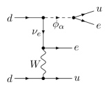
Refer to caption
(a) Long-range contribution
Refer to caption
(b) Short-range contribution
Figure 7: New contributions to neutrinoless double beta-decay.

The couplings of the leptoquark contributing to neutrinoless double beta-decay, i.e. 𝝀𝒊𝟏𝜶𝑳𝑸subscriptsuperscript𝝀𝑳𝑸𝒊1𝜶\lambda^{LQ}_{i1\alpha}, 𝝀𝒊𝟏𝜶𝒆𝒖subscriptsuperscript𝝀𝒆𝒖𝒊1𝜶\lambda^{eu}_{i1\alpha} as well as 𝝀𝟏𝜶𝒅𝒇subscriptsuperscript𝝀𝒅𝒇1𝜶\lambda^{df}_{1\alpha}, do not enter the expression for neutrino masses and thus are not constrained from below and can be arbitrary without affecting the neutrino mass contribution. Hence, we are left with the standard contribution from light neutrinos. The magnitude of the effective mass controlling the light neutrino contribution to neutrinoless double beta decay is given by

𝒎𝒆𝒆=𝑼𝒆𝒊𝟐𝒎𝒊.delimited-⟨⟩subscript𝒎𝒆𝒆superscriptsubscript𝑼𝒆𝒊2subscript𝒎𝒊\left\langle m_{ee}\right\rangle=\sum U_{ei}^{2}m_{i}\ . (5.12)

As the mass of the lightest neutrino almost vanishes, we read off 𝒎𝒆𝒆(0.2𝟒)×𝟏𝟎𝟑𝐞𝐕similar-to-or-equalsdelimited-⟨⟩subscript𝒎𝒆𝒆0.24superscript103𝐞𝐕\left\langle m_{ee}\right\rangle\simeq(0.2-4)\times 10^{-3}\,\mathrm{eV} [(𝟏𝟒)×𝟏𝟎𝟐𝐞𝐕14superscript102𝐞𝐕(1-4)\times 10^{-2}\,\mathrm{eV}] for 𝒎𝟏𝟎𝐞𝐕similar-to-or-equalssubscript𝒎10𝐞𝐕m_{1}\simeq 0\,\mathrm{eV} from Fig. 2 in [84] in case of a normal [inverted] mass ordering varying the other neutrino mass parameters in their 𝟑𝝈3𝝈3\sigma ranges. Concluding, there are currently no constraints from neutrinoless double beta decay on the parameter space of this model.

6 Collider Constraints

As there are several new particles in the model, which might have masses close to the electroweak scale, they can be searched for at colliders. In particular, hadron colliders, like the LHC, seem promising, because all new particles carry color charge and therefore couple to gluons. We will not perform a detailed collider study, since it is beyond the scope of this paper and thus left for future work, but we will discuss the different search channels for the scalar leptoquark and the fermionic colored octet in the following subsections.

6.1 Scalar Leptoquark

The scalar leptoquark ϕ𝜶subscriptbold-italic-ϕ𝜶\phi_{\alpha} is mainly pair-produced in gluon fusion as well as 𝒒𝒒¯𝒒bold-¯𝒒q\bar{q} annihilation, while the production via the exchange of leptons through Yukawa interactions is suppressed. The main pair production channels are shown in Fig. 8. There are more pair-production channels; however, they rely on Yukawa couplings to the first generation of quarks, which are highly constrained by flavor physics, as we discussed in Sec. 5. Besides pair production, the leptoquark ϕ𝜶subscriptbold-italic-ϕ𝜶\phi_{\alpha} can also be singly produced via its Yukawa interactions 𝝀𝑳𝑸,𝒆𝒖superscript𝝀𝑳𝑸𝒆𝒖\lambda^{LQ,eu}, but they are similarly suppressed compared to the pair-production channels relying on Yukawa couplings.
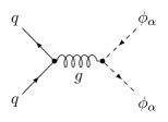
Refer to caption
(a)
Refer to caption
(b)
Refer to caption
(c)
Refer to caption
(d)
Refer to caption
(e)
Figure 8: Main pair production channels for leptoquarks

The leptoquark will decay into either a down-type, mostly 𝒃𝒃b, quark and a neutrino or a top quark and a charged lepton. The decay into 𝒃𝒃b quark plus missing transverse energy (MET) resembles the standard direct sbottom pair production search, but with a reduced branching fraction for 𝒎ϕ𝜶>𝒎𝒕subscript𝒎subscriptbold-italic-ϕ𝜶subscript𝒎𝒕m_{\phi_{\alpha}}>m_{t}. Hence, the possible collider signatures are two 𝒃𝒃b-jets plus MET, leptons and/or additional jets in the final state. The leptoquarks in this model differ from the standard assumption in leptoquark searches that the leptoquark couples to one generation only. Due to the flavor structure of the neutrino mass matrix, the leptoquark has to couple to the third generation of left-handed quarks as well as all three generations of left-handed leptons. The couplings to the right-handed particles as well as the first two generations of left-handed quarks are not required in order to generate neutrino masses and therefore can be arbitrarily small. In fact, the couplings to the first two generations of quarks are strongly constrained by collider searches and especially flavor physics constraints, as we discussed in Sec. 5.

The CMS Collaboration has performed a search for two 𝒃𝒃b-jets plus MET, leptons and/or additional jets in the final state, based on 4.7 fb-1 of 𝒔=𝒔absent\sqrt{s}=7 TeV data [85]. The analysis sets a lower limit on 𝒎ϕsubscript𝒎bold-italic-ϕm_{\phi} of 450 GeV assuming a 100% branching fraction to a 𝒃𝒃b-quark and a 𝝉𝝉\tau-neutrino. However the limit from this search is much lower for realistic branching fractions, since the branching fraction decreases from 𝟏𝟎𝟎%percent100100\% for leptoquarks lighter than the top quark down to 𝟓𝟎%percent5050\% for a leptoquark mass much heavier than the top quark. In our model, we expect a limit slightly above the top mass. Nonetheless this situation is certain to change with increased data and the LHC should be able to provide important constraints on this model. A detailed study is left for future work.

6.2 Fermionic Colored Octet

The fermionic colored octet 𝒇𝒇f is pair-produced similarly to a gluino, dominantly via gluon fusion. The main production channels are shown in Fig. 9.
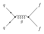
Refer to caption
(a)
Refer to caption
(b)
Refer to caption
(c)
Refer to caption
(d)
Figure 9: Pair production channels of the fermionic colored octet

It decays via the coupling 𝝀𝒅𝒇superscript𝝀𝒅𝒇\lambda^{df} into a down-type, mostly 𝒃𝒃b-, quark and a leptoquark, which decays via the interactions 𝝀𝑳𝑸,𝒆𝒖superscript𝝀𝑳𝑸𝒆𝒖\lambda^{LQ,eu} to either a 𝒃𝒃b-quark and a neutrino or a top quark and a charged lepton,

𝒇𝒃ϕ𝒃𝒃𝝂,𝐚𝐧𝐝𝒇𝒃ϕ𝒃𝒕.formulae-sequencebold-→𝒇𝒃superscriptbold-italic-ϕbold-†bold-→𝒃𝒃𝝂bold-→𝐚𝐧𝐝𝒇𝒃superscriptbold-italic-ϕbold-†bold-→𝒃𝒕bold-ℓf\to b\phi^{\dagger}\to bb\nu\ ,\quad\mathrm{and}\quad f\to b\phi^{\dagger}\to bt\ell\ . (6.1)

The top quark decays in the usual way into a 𝑾𝑾W boson and a 𝒃𝒃b-quark and therefore leads to another 𝒃𝒃b-jet in the final state as well as additional jets, or a lepton and MET. Depending on the masses, the decays are via off-shell particles. Hence the final state contains four 𝒃𝒃b-jets and depending on the decay channel MET, leptons and/or additional jets. As the fermionic colored octet is a Majorana fermion, it can lead to a fermion number violating process and lead to like-sign top as well as lepton pairs in the final state, which are ideal channels to search for new physics due to the small SM background. Due to the similarity of production as well as some of the decay channels with a gluino, we expect that the LHC experiments should be already able to produce reasonable constraints on the colored fermionic octet. However, none of the current searches is directly applicable without a simulation.

In order to set a limit on 𝒎𝒇subscript𝒎𝒇m_{f}, a recent gluino search from the CMS Collaboration could be exploited [86; *Chatrchyan:2012paa]. This result is useful as they present the raw numbers obtained at a number of intermediate steps in the analysis, which would allow the differences between our present model and the SUSY gluino scenario to be accounted for. Despite this, we have not done this in the present paper for pragmatic reasons. As seen in Sec. 3, the neutrino mass generated in our model is only weakly dependent on 𝒎𝒇subscript𝒎𝒇m_{f}, and derived limits are unlikely to meaningfully constrain the model. Future searches may alter this conclusion, but the more interesting constraint colliders can place on this model is through 𝒎ϕ𝜶subscript𝒎subscriptbold-italic-ϕ𝜶m_{\phi_{\alpha}}.

7 Naturalness Constraints

As there are three scalars in the model, we have to discuss the effects of quadratic corrections to the scalar masses from other particles. We will firstly consider the contributions of the scalar leptoquarks as well as the fermionic colored octet to the SM Higgs and then calculate the quadratic correction to the leptoquark masses.

7.1 Contributions to the SM Higgs

The newly introduced particles, the colored octet fermion as well as the two leptoquarks, contribute to the effective Higgs potential. For completeness, we give the tree-level Higgs potential

𝑽=𝝁𝟐𝑯𝑯+𝝀(𝑯𝑯)𝟐𝑽superscript𝝁2superscript𝑯bold-†𝑯𝝀superscriptsuperscript𝑯bold-†𝑯2V=-\mu^{2}H^{\dagger}H+\lambda(H^{\dagger}H)^{2} (7.1)

and therefore the VEV 𝑯delimited-⟨⟩𝑯\left\langle H\right\rangle and the Higgs mass 𝒎𝒉𝟐superscriptsubscript𝒎𝒉2m_{h}^{2} are given by

𝑯𝟐=𝝁𝟐𝟐𝝀,𝐚𝐧𝐝𝒎𝒉𝟐=𝟒𝝁𝟐=𝟖𝝀𝑯𝟐.formulae-sequencesuperscriptdelimited-⟨⟩𝑯2superscript𝝁22𝝀𝐚𝐧𝐝superscriptsubscript𝒎𝒉24superscript𝝁28𝝀superscriptdelimited-⟨⟩𝑯2\left\langle H\right\rangle^{2}=\frac{\mu^{2}}{2\lambda}\ ,\quad\mathrm{and}\quad m_{h}^{2}=4\mu^{2}=8\lambda\left\langle H\right\rangle^{2}\ . (7.2)

We are especially interested in corrections to the mass terms, since they are quadratically sensitive to the new mass scales. Even setting all new couplings which do not enter the neutrino mass contribution to zero at some scale, there is a contribution dependent on the parameters 𝝀𝒊𝟑𝜶𝑳𝑸subscriptsuperscript𝝀𝑳𝑸𝒊3𝜶\lambda^{LQ}_{i3\alpha} as well as 𝝀𝟑𝜶𝒅𝒇subscriptsuperscript𝝀𝒅𝒇3𝜶\lambda^{df}_{3\alpha} at two-loop order,

|𝒚𝒃|𝟐(𝟒𝝅)𝟒𝜶[𝟑𝒊|𝝀𝒊𝟑𝜶𝑳𝑸|𝟐𝒇𝟏(𝒎ϕ𝜶𝟐)+𝟒|𝝀𝟑𝜶𝒅𝒇|𝟐𝒇𝟐(𝒎ϕ𝜶𝟐,𝒎𝒇𝟐)]𝑯𝑯,superscriptsubscript𝒚𝒃2superscript4𝝅4subscript𝜶delimited-[]3subscript𝒊superscriptsubscriptsuperscript𝝀𝑳𝑸𝒊3𝜶2subscript𝒇1superscriptsubscript𝒎subscriptbold-italic-ϕ𝜶24superscriptsubscriptsuperscript𝝀𝒅𝒇3𝜶2subscript𝒇2superscriptsubscript𝒎subscriptbold-italic-ϕ𝜶2superscriptsubscript𝒎𝒇2superscript𝑯bold-†𝑯-\frac{|y_{b}|^{2}}{(4\pi)^{4}}\sum_{\alpha}\left[3\,\sum_{i}\left|\lambda^{LQ}_{i3\alpha}\right|^{2}f_{1}(m_{\phi_{\alpha}}^{2})+4\,\left|\lambda^{df}_{3\alpha}\right|^{2}f_{2}(m_{\phi_{\alpha}}^{2},m_{f}^{2})\right]H^{\dagger}H\ , (7.3)

where the functions 𝒇𝒊subscript𝒇𝒊f_{i} encode the structure of the two-loop diagram. The relevant diagrams are shown in Fig. 10.
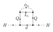
Refer to caption
(a) Relevant contribution proportional to (𝝀𝑳𝑸)𝟐superscriptsuperscript𝝀𝑳𝑸2(\lambda^{LQ})^{2}.
Refer to caption
(b) Relevant contribution proportional to (𝝀𝒅𝒇)𝟐superscriptsuperscript𝝀𝒅𝒇2(\lambda^{df})^{2}.
Figure 10: Different contributions to the effective Higgs potential

We will use this contribution to estimate the natural region of parameter space, where the contribution to the Higgs mass is less than 𝟏𝟐𝟔𝐆𝐞𝐕126𝐆𝐞𝐕126\,\mathrm{GeV}, the measured value of the resonance at the LHC:

𝟏𝟐|𝒚𝒃|𝟐(𝟒𝝅)𝟒𝒊|𝝀𝒊𝟑𝜶𝑳𝑸|𝟐𝒎ϕ𝜶𝟐12superscriptsubscript𝒚𝒃2superscript4𝝅4subscript𝒊superscriptsubscriptsuperscript𝝀𝑳𝑸𝒊3𝜶2superscriptsubscript𝒎subscriptbold-italic-ϕ𝜶2\displaystyle\frac{12|y_{b}|^{2}}{(4\pi)^{4}}\sum_{i}\left|\lambda^{LQ}_{i3\alpha}\right|^{2}m_{\phi_{\alpha}}^{2} 𝟒𝝁𝟐=𝒎𝒉𝟐less-than-or-similar-toabsent4superscript𝝁2superscriptsubscript𝒎𝒉2\displaystyle\lesssim 4\mu^{2}=m_{h}^{2} bold-⇒\displaystyle\Rightarrow 𝒎ϕ𝜶𝟏𝟗𝟎𝟎𝒊|𝝀𝒊𝟑𝜶𝑳𝑸|𝟐𝒎𝒉less-than-or-similar-tosubscript𝒎subscriptbold-italic-ϕ𝜶1900subscript𝒊superscriptsubscriptsuperscript𝝀𝑳𝑸𝒊3𝜶2subscript𝒎𝒉\displaystyle m_{\phi_{\alpha}}\lesssim\frac{1900}{\sqrt{\sum_{i}\left|\lambda^{LQ}_{i3\alpha}\right|^{2}}}m_{h} (7.4a)
𝟏𝟔|𝒚𝒃|𝟐(𝟒𝝅)𝟒|𝝀𝟑𝜶𝒅𝒇|𝟐𝐦𝐚𝐱(𝒎ϕ𝜶𝟐,𝒎𝒇𝟐)16superscriptsubscript𝒚𝒃2superscript4𝝅4superscriptsubscriptsuperscript𝝀𝒅𝒇3𝜶2superscriptsubscript𝒎subscriptbold-italic-ϕ𝜶2superscriptsubscript𝒎𝒇2\displaystyle\frac{16|y_{b}|^{2}}{(4\pi)^{4}}\left|\lambda^{df}_{3\alpha}\right|^{2}\max(m_{\phi_{\alpha}}^{2},m_{f}^{2}) 𝟒𝝁𝟐=𝒎𝒉𝟐less-than-or-similar-toabsent4superscript𝝁2superscriptsubscript𝒎𝒉2\displaystyle\lesssim 4\mu^{2}=m_{h}^{2} bold-⇒\displaystyle\Rightarrow 𝒎ϕ𝜶,𝒎𝒇𝟏𝟔𝟎𝟎|𝝀𝟑𝜶𝒅𝒇|𝒎𝒉,less-than-or-similar-tosubscript𝒎subscriptbold-italic-ϕ𝜶subscript𝒎𝒇1600subscriptsuperscript𝝀𝒅𝒇3𝜶subscript𝒎𝒉\displaystyle m_{\phi_{\alpha}},m_{f}\lesssim\frac{1600}{\left|\lambda^{df}_{3\alpha}\right|}m_{h}\ , (7.4b)

where we assumed that the loop functions 𝒇𝒊(𝒎𝟐)𝒎𝟐similar-tosubscript𝒇𝒊superscript𝒎2superscript𝒎2f_{i}(m^{2})\sim m^{2}. Similarly, at three-loop order, there are contributions to the quartic Higgs coupling. However, they are too small to lead to any competitive constraints. Summarizing, naturalness prefers smaller masses of the new particles.

7.2 Naturalness of the Leptoquark Masses

Similarly to the Higgs mass, the mass term of the leptoquark receives corrections to its mass. The most important diagrams are shown in Fig. 11. We can readily estimate the contribution due to the fermionic colored octet 𝒇𝒇f

(𝜹𝒎ϕ𝟐)𝜶𝜷=𝟒𝟑𝝀𝟑𝜶𝒅𝒇𝝀𝟑𝜷𝒅𝒇𝟏𝟔𝝅𝟐𝑨𝟎[𝒎𝒇𝟐]𝒎𝒇𝟐𝟑𝝅|𝝀𝟑𝜶𝒅𝒇|𝒎ϕ𝜶subscript𝜹superscriptsubscript𝒎bold-italic-ϕ2𝜶𝜷43subscriptsuperscript𝝀𝒅𝒇3𝜶subscriptsuperscript𝝀𝒅𝒇3𝜷16superscript𝝅2subscript𝑨0delimited-[]superscriptsubscript𝒎𝒇2bold-⇒subscript𝒎𝒇less-than-or-similar-to23𝝅subscriptsuperscript𝝀𝒅𝒇3𝜶subscript𝒎subscriptbold-italic-ϕ𝜶(\delta m_{\phi}^{2})_{\alpha\beta}=-\frac{4}{3}\frac{\lambda^{df}_{3\alpha}\lambda^{df*}_{3\beta}}{16\pi^{2}}A_{0}[m_{f}^{2}]\Rightarrow m_{f}\lesssim\frac{2\sqrt{3}\pi}{\left|\lambda^{df}_{3\alpha}\right|}m_{\phi_{\alpha}} (7.5)

and therefore the hierarchy between the leptoquark masses and the colored octet mass is limited by naturalness depending on the coupling 𝝀𝒅𝒇superscript𝝀𝒅𝒇\lambda^{df}. Similarly, the hierarchy between the leptoquark masses itself is limited by naturalness

(𝜹𝒎ϕ𝟐)𝜶𝜷=𝜸,𝒊,𝒋𝝀𝒋𝟑𝜶𝑳𝑸𝝀𝒋𝟑𝜷𝑳𝑸(𝟒𝝅)𝟒|𝝀𝒊𝟑𝜸𝑳𝑸|𝟐𝒉𝟏(𝒎ϕ𝜸𝟐)𝒎ϕ𝜸𝟏𝟔𝝅𝟐𝒊,𝒋|𝝀𝒋𝟑𝜶𝑳𝑸𝝀𝒊𝟑𝜸𝑳𝑸|𝟐𝒎ϕ𝜶,subscript𝜹superscriptsubscript𝒎bold-italic-ϕ2𝜶𝜷subscript𝜸𝒊𝒋subscriptsuperscript𝝀𝑳𝑸𝒋3𝜶subscriptsuperscript𝝀𝑳𝑸𝒋3𝜷superscript4𝝅4superscriptsubscriptsuperscript𝝀𝑳𝑸𝒊3𝜸2subscript𝒉1superscriptsubscript𝒎subscriptbold-italic-ϕ𝜸2bold-⇒subscript𝒎subscriptbold-italic-ϕ𝜸less-than-or-similar-to16superscript𝝅2subscript𝒊𝒋superscriptsubscriptsuperscript𝝀𝑳𝑸𝒋3𝜶subscriptsuperscript𝝀𝑳𝑸𝒊3𝜸2subscript𝒎subscriptbold-italic-ϕ𝜶(\delta m_{\phi}^{2})_{\alpha\beta}=-\sum_{\gamma,i,j}\frac{\lambda^{LQ}_{j3\alpha}\lambda^{LQ}_{j3\beta}}{(4\pi)^{4}}\left|\lambda^{LQ}_{i3\gamma}\right|^{2}h_{1}(m_{\phi_{\gamma}}^{2})\Rightarrow m_{\phi_{\gamma}}\lesssim\frac{16\pi^{2}}{\sqrt{\sum_{i,j}|\lambda^{LQ}_{j3\alpha}\lambda^{LQ}_{i3\gamma}|^{2}}}m_{\phi_{\alpha}}\ , (7.6)

where 𝒉𝟏subscript𝒉1h_{1} encodes the loop integral structure. We do not take into account any corrections to the quartic interactions, since they do not lead to any competitive constraints. Concluding, naturalness disfavors a large hierarchy in the masses of the new particles.

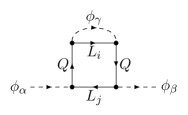
Refer to caption
(a) Relevant contribution proportional to (𝝀𝒅𝒇)𝟐superscriptsuperscript𝝀𝒅𝒇2(\lambda^{df})^{2}.
Refer to caption
(b) Relevant contribution proportional to (𝝀𝑳𝑸)𝟒superscriptsuperscript𝝀𝑳𝑸4(\lambda^{LQ})^{4}.
Figure 11: Different contributions to the effective potential of the leptoquark

8 Mathematica Code

Together with this paper, we publish the Mathematica package ANT, which provides all Passarino-Veltman (PV) functions up to boxes in the limit of vanishing external momenta using the definitions of FormCalc/LoopTools [49]. In addition, it includes all first derivatives with respect to the external momenta of the following PV functions

𝑩𝟎,𝑩𝟏,𝑪𝟎,𝑪𝟏,𝑪𝟐,𝐚𝐧𝐝𝑪𝟎𝟎,subscript𝑩0subscript𝑩1subscript𝑪0subscript𝑪1subscript𝑪2𝐚𝐧𝐝subscript𝑪00B_{0},\quad B_{1},\quad C_{0},\quad C_{1},\quad C_{2},\quad\mathrm{and}\quad C_{00}\;,

which were necessary for the calculations in this work. See Appendix C for the list of all PV functions contained in the Mathematica package. After loading the Mathematica package, the function ANT is available, which can be used to evaluate an arbitrary expression containing PV functions given in the limit of vanishing external momenta. Besides the function ANT, it defines the functions A0ant, B0ant, C0ant, and D0ant, which directly evaluate to the result for the corresponding functions A0, B0i, C0i, and D0i, respectively, in the given limit. The package ANT can be downloaded from http://ant.hepforge.org.

In order to illustrate the use of ANT, we give one short example and refer the interested reader to the documentation for further information. The following example code

<< ANT.m;
expr=a + b C0i[cc0,0,0,0,m1s,m2s,0];
ANT[expr]

leads to the output

𝒂+𝒃𝟐m1s𝟐𝐥𝐨𝐠(m2s)+𝟑m1s𝟐𝟐m1s𝟐𝐥𝐨𝐠(m1s)𝟒m1sm2s+m2s𝟐𝟔(m1sm2s)𝟑.𝒂𝒃2superscriptm1s2m2s3superscriptm1s22superscriptm1s2m1s4m1sm2ssuperscriptm2s26superscriptm1sm2s3a+b\,\frac{2\,\text{m1s}^{2}\log(\text{m2s})+3\,\text{m1s}^{2}-2\,\text{m1s}^{2}\,\log(\text{m1s})-4\,\text{m1s}\,\text{m2s}+\text{m2s}^{2}}{6\,(\text{m1s}-\text{m2s})^{3}}\;.

9 Summary and Conclusions

The origin of neutrino masses and mixings is one of the most important topics in physics beyond the standard model. The three well-known see-saw models are tree-level scenarios for Majorana neutrino mass generation that lie at one end of a whole sequence of possible models. Viewing these theories from the vantage point of gauge-invariant and baryon-symmetric effective operators that violate lepton number conservation by two units, the see-saw models are seen to be the simplest UV completions of the dimension-5 Weinberg operator 𝑳𝑳𝑯𝑯𝑳𝑳𝑯𝑯LLHH. The other models in the sequence are based on more complicated effective operators, and they necessarily feature radiative neutrino mass generation. We have constructed and thoroughly analyzed the constraints on a new model of this kind, based on a certain UV completion of an effective operator with flavor structure 𝑳𝑳𝑸𝒅𝒄𝑸𝒅𝒄𝑳𝑳𝑸superscript𝒅𝒄𝑸superscript𝒅𝒄LLQd^{c}Qd^{c}. This is the first time, to our knowledge, that a radiative neutrino mass model involving exotic fermions in addition to exotic scalars has been so exhaustively studied. Neutrino masses and mixings are generated at 2-loop level using a Majorana color-octet fermion and two copies of a color-triplet, isosinglet, charge 𝟏/𝟑13-1/3 leptoquark scalar.

Fitting the parameters to reproduce the observed neutrino masses and mixings, we then derived the constraints on the remaining parameter space from various, mainly flavor-changing processes. We focused on the region of parameter space where the only relevant Yukawa couplings were to the third generation. We found that the lepton-flavor-violating processes of 𝝁𝝁\mu to 𝒆𝒆e conversion in nuclei, 𝝁𝒆𝜸bold-→𝝁𝒆𝜸\mu\to e\gamma and 𝝁𝒆𝒆𝒆bold-→𝝁𝒆𝒆𝒆\mu\to eee provided the most stringent constraints, as summarized in Figs. 4-6. We also derived bounds from other processes – exotic contributions to 𝒁𝒁Z and 𝒕𝒕t decay, neutral-meson mixing, 𝒃𝒔𝜸bold-→𝒃𝒔𝜸b\to s\gamma – that turned out to less constraining on the parameters of this particular model. Finally, we estimated bounds on Yukawa coupling constants that play no role in the generation of neutrino mass but are required by the theory to exist. These included the couplings of the leptoquarks to right-handed up-type quarks and charged leptons, and other Yukawa couplings to the first two generations of quarks and leptons.

Collider constraints were also examined. While the leptoquarks have the same quantum numbers as right-handed sbottoms, and similar states have in general have been searched for at the LHC, currently no useful collider bounds exist. The reason is that the characteristic leptoquark decay branching ratios in this model, as driven by their role in neutrino mass generation, place them out of view of current searches. This situation is expected to change in the future, however. The exotic fermion resembles a gluino, but since the neutrino masses and mixings do not depend critically on its mass, current collider constraints are not significant.

The dashed black lines in Figs. 4-6 show expected sensitivities of future experiments. Clearly, the best prospects lie in the quite significant improvements expected in 𝝁𝝁\mu to 𝒆𝒆e conversion measurements [63; *Cui:2009zz]. In addition, it would be very useful to extend the scope of LHC searches for leptoquark scalars to encompass a wider range of decay mode branching ratios.

Acknowledgements

We thank K. S. Babu, Y. Bai, I. Baldes, J. Barnard, T. Gherghetta, A. de Gouvêa, K. McDonald, B. McKellar and M. White for many very useful discussions. We thank L. Silvestrini for providing a constraint on 𝑪𝚫𝒎𝑲subscript𝑪𝚫subscript𝒎𝑲C_{\Delta m_{K}} and explaining why it has been removed from the list. We thank D. Straub for pointing out a mistake in the previous version. This work was supported in part by the Australian Research Council.

Appendix A More Details of Flavor Physics

In this section, we summarize general formula for the contributions to LFV rare decays involving left- as well as right-handed couplings.

A.1 𝒍𝒊𝒍𝒋𝜸bold-→subscript𝒍𝒊subscript𝒍𝒋𝜸l_{i}\to l_{j}\gamma

Contributions to 𝒍𝒊𝒍𝒋𝜸bold-→subscript𝒍𝒊subscript𝒍𝒋𝜸l_{i}\to l_{j}\gamma from left- as well as right-handed couplings to the third generation of quarks are given by

𝝈𝑳𝒊𝒋=subscript𝝈𝑳𝒊𝒋absent\displaystyle\sigma_{Lij}= 𝟏𝟏𝟔𝝅𝟐𝒂=𝟏𝟑𝒎=𝟏𝟐𝝀𝒊𝒂𝒎𝑳𝑸𝝀𝒋𝒂𝒎𝑳𝑸𝒎𝒍𝒊+𝝀𝒊𝒂𝒎𝒆𝒖𝝀𝒋𝒂𝒎𝒆𝒖𝒎𝒍𝒋𝒎ϕ𝒎𝟐𝟏+𝟒𝒕𝒂𝒎𝟓𝒕𝒂𝒎𝟐+𝟐𝒕𝒂𝒎(𝟐+𝒕𝒂𝒎)𝐥𝐧𝒕𝒂𝒎𝟒(𝒕𝒂𝒎𝟏)𝟒116superscript𝝅2superscriptsubscript𝒂13superscriptsubscript𝒎12superscriptsubscript𝝀𝒊𝒂𝒎𝑳𝑸superscriptsubscript𝝀𝒋𝒂𝒎𝑳𝑸bold-†subscript𝒎subscript𝒍𝒊superscriptsubscript𝝀𝒊𝒂𝒎𝒆𝒖superscriptsubscript𝝀𝒋𝒂𝒎𝒆𝒖bold-†subscript𝒎subscript𝒍𝒋superscriptsubscript𝒎subscriptbold-italic-ϕ𝒎214subscript𝒕𝒂𝒎5superscriptsubscript𝒕𝒂𝒎22subscript𝒕𝒂𝒎2subscript𝒕𝒂𝒎subscript𝒕𝒂𝒎4superscriptsubscript𝒕𝒂𝒎14\displaystyle\frac{1}{16\pi^{2}}\sum_{a=1}^{3}\sum_{m=1}^{2}\frac{\lambda_{iam}^{LQ}\lambda_{jam}^{LQ\dagger}m_{l_{i}}+\lambda_{iam}^{eu}\lambda_{jam}^{eu\dagger}m_{l_{j}}}{m_{\phi_{m}}^{2}}\frac{1+4t_{am}-5t_{am}^{2}+2t_{am}(2+t_{am})\ln t_{am}}{4(t_{am}-1)^{4}}
+\displaystyle+ 𝟏𝟏𝟔𝝅𝟐𝒂=𝟏𝟑𝒎=𝟏𝟐𝝀𝒊𝒂𝒎𝑳𝑸𝝀𝒋𝒂𝒎𝒆𝒖𝒎𝒖𝒂𝒎ϕ𝒎𝟐𝟕𝟖𝒕𝒂𝒎+𝒕𝒂𝒎𝟐+𝟐(𝟐+𝒕𝒂𝒎)𝐥𝐧𝒕𝒂𝒎𝟐(𝒕𝒂𝒎𝟏)𝟑,116superscript𝝅2superscriptsubscript𝒂13superscriptsubscript𝒎12superscriptsubscript𝝀𝒊𝒂𝒎𝑳𝑸superscriptsubscript𝝀𝒋𝒂𝒎𝒆𝒖bold-†subscript𝒎subscript𝒖𝒂superscriptsubscript𝒎subscriptbold-italic-ϕ𝒎278subscript𝒕𝒂𝒎superscriptsubscript𝒕𝒂𝒎222subscript𝒕𝒂𝒎subscript𝒕𝒂𝒎2superscriptsubscript𝒕𝒂𝒎13\displaystyle\frac{1}{16\pi^{2}}\sum_{a=1}^{3}\sum_{m=1}^{2}\frac{\lambda_{iam}^{LQ}\lambda_{jam}^{eu\dagger}m_{u_{a}}}{m_{\phi_{m}}^{2}}\frac{7-8t_{am}+t_{am}^{2}+2(2+t_{am})\ln t_{am}}{2(t_{am}-1)^{3}}\ , (A.1a)
𝝈𝑹𝒊𝒋=subscript𝝈𝑹𝒊𝒋absent\displaystyle\sigma_{Rij}= 𝟏𝟏𝟔𝝅𝟐𝒂=𝟏𝟑𝒎=𝟏𝟐𝝀𝒊𝒂𝒎𝑳𝑸𝝀𝒋𝒂𝒎𝑳𝑸𝒎𝒍𝒋+𝝀𝒊𝒂𝒎𝒆𝒖𝝀𝒋𝒂𝒎𝒆𝒖𝒎𝒍𝒊𝒎ϕ𝒎𝟐𝟏+𝟒𝒕𝒂𝒎𝟓𝒕𝒂𝒎𝟐+𝟐𝒕𝒂𝒎(𝟐+𝒕𝒂𝒎)𝐥𝐧𝒕𝒂𝒎𝟒(𝒕𝒂𝒎𝟏)𝟒116superscript𝝅2superscriptsubscript𝒂13superscriptsubscript𝒎12superscriptsubscript𝝀𝒊𝒂𝒎𝑳𝑸superscriptsubscript𝝀𝒋𝒂𝒎𝑳𝑸bold-†subscript𝒎subscript𝒍𝒋superscriptsubscript𝝀𝒊𝒂𝒎𝒆𝒖superscriptsubscript𝝀𝒋𝒂𝒎𝒆𝒖bold-†subscript𝒎subscript𝒍𝒊superscriptsubscript𝒎subscriptbold-italic-ϕ𝒎214subscript𝒕𝒂𝒎5superscriptsubscript𝒕𝒂𝒎22subscript𝒕𝒂𝒎2subscript𝒕𝒂𝒎subscript𝒕𝒂𝒎4superscriptsubscript𝒕𝒂𝒎14\displaystyle\frac{1}{16\pi^{2}}\sum_{a=1}^{3}\sum_{m=1}^{2}\frac{\lambda_{iam}^{LQ}\lambda_{jam}^{LQ\dagger}m_{l_{j}}+\lambda_{iam}^{eu}\lambda_{jam}^{eu\dagger}m_{l_{i}}}{m_{\phi_{m}}^{2}}\frac{1+4t_{am}-5t_{am}^{2}+2t_{am}(2+t_{am})\ln t_{am}}{4(t_{am}-1)^{4}}
+\displaystyle+ 𝟏𝟏𝟔𝝅𝟐𝒂=𝟏𝟑𝒎=𝟏𝟐𝝀𝒊𝒂𝒎𝒆𝒖𝝀𝒋𝒂𝒎𝑳𝑸𝒎𝒖𝒂𝒎ϕ𝒎𝟐𝟕𝟖𝒕𝒂𝒎+𝒕𝒂𝒎𝟐+𝟐(𝟐+𝒕𝒂𝒎)𝐥𝐧𝒕𝒂𝒎𝟐(𝒕𝒂𝒎𝟏)𝟑,116superscript𝝅2superscriptsubscript𝒂13superscriptsubscript𝒎12superscriptsubscript𝝀𝒊𝒂𝒎𝒆𝒖superscriptsubscript𝝀𝒋𝒂𝒎𝑳𝑸bold-†subscript𝒎subscript𝒖𝒂superscriptsubscript𝒎subscriptbold-italic-ϕ𝒎278subscript𝒕𝒂𝒎superscriptsubscript𝒕𝒂𝒎222subscript𝒕𝒂𝒎subscript𝒕𝒂𝒎2superscriptsubscript𝒕𝒂𝒎13\displaystyle\frac{1}{16\pi^{2}}\sum_{a=1}^{3}\sum_{m=1}^{2}\frac{\lambda_{iam}^{eu}\lambda_{jam}^{LQ\dagger}m_{u_{a}}}{m_{\phi_{m}}^{2}}\frac{7-8t_{am}+t_{am}^{2}+2(2+t_{am})\ln t_{am}}{2(t_{am}-1)^{3}}\ , (A.1b)

where 𝒕𝒂𝒎=𝒎𝒖𝒂𝟐/𝒎ϕ𝒎𝟐subscript𝒕𝒂𝒎superscriptsubscript𝒎subscript𝒖𝒂2superscriptsubscript𝒎subscriptbold-italic-ϕ𝒎2t_{am}=m_{u_{a}}^{2}/m_{\phi_{m}}^{2} and 𝒎𝒖𝒂subscript𝒎subscript𝒖𝒂m_{u_{a}} is the mass of the appropriate up-type quark mass.

A.2 𝝁𝒆𝒆+𝒆bold-→superscript𝝁superscript𝒆superscript𝒆superscript𝒆\mu^{-}\to e^{-}e^{+}e^{-}

In this subsection, we list the different contributions to 𝝁𝒆𝒆+𝒆+bold-→superscript𝝁superscript𝒆superscript𝒆superscript𝒆\mu^{-}\to e^{-}e^{+}e^{+} from left- as well as right-handed couplings to the third generation of quarks

𝑨𝟏𝑳,𝑹superscriptsubscript𝑨1𝑳𝑹\displaystyle A_{1}^{L,R} =\displaystyle= 𝒂=𝟏𝟑𝒎=𝟏𝟐𝝀𝟐𝒂𝒎𝑳𝑸,𝒆𝒖𝝀𝟏𝒂𝒎𝑳𝑸,𝒆𝒖𝟑𝟖𝟒𝝅𝟐𝒎ϕ𝒎𝟐superscriptsubscript𝒂13superscriptsubscript𝒎12subscriptsuperscript𝝀𝑳𝑸𝒆𝒖2𝒂𝒎subscriptsuperscript𝝀𝑳𝑸𝒆𝒖bold-†1𝒂𝒎384superscript𝝅2superscriptsubscript𝒎subscriptbold-italic-ϕ𝒎2\displaystyle\sum_{a=1}^{3}\sum_{m=1}^{2}\frac{\lambda^{LQ,eu}_{2am}\lambda^{LQ,eu\dagger}_{1am}}{384\pi^{2}m_{\phi_{m}}^{2}} (A.2a)
×\displaystyle\times (𝒕𝒂𝒎𝟏)(𝟏𝟎+(𝟏𝟕+𝒕𝒂𝒎)𝒕𝒂𝒎)𝟐(𝟒𝟔𝒕𝒂𝒎𝒕𝒂𝒎𝟑)𝐥𝐧𝒕𝒂𝒎(𝒕𝒂𝒎𝟏)𝟒,subscript𝒕𝒂𝒎11017subscript𝒕𝒂𝒎subscript𝒕𝒂𝒎246subscript𝒕𝒂𝒎superscriptsubscript𝒕𝒂𝒎3subscript𝒕𝒂𝒎superscriptsubscript𝒕𝒂𝒎14\displaystyle\frac{\left(t_{am}-1\right)\left(10+\left(-17+t_{am}\right)t_{am}\right)-2\left(4-6t_{am}-t_{am}^{3}\right)\ln t_{am}}{(t_{am}-1)^{4}}\ ,
𝑨𝟐𝑳,𝑹superscriptsubscript𝑨2𝑳𝑹\displaystyle A_{2}^{L,R} =\displaystyle= 𝝈𝑳𝟐𝟏,𝑹𝟐𝟏𝒎𝝁,subscript𝝈𝑳21𝑹21subscript𝒎𝝁\displaystyle\frac{\sigma_{L21,R21}}{m_{\mu}}\ , (A.2b)
𝑭𝑳,𝑹subscript𝑭𝑳𝑹\displaystyle F_{L,R} =\displaystyle= 𝒂=𝟏𝟑𝒎=𝟏𝟐𝟑𝒆𝝀𝟐𝒂𝒎𝑳𝑸,𝒆𝒖𝝀𝟏𝒂𝒎𝑳𝑸,𝒆𝒖𝟑𝟐𝝅𝟑𝐬𝐢𝐧𝜽𝑾𝐜𝐨𝐬𝜽𝑾𝒕𝒂𝒎(𝟏𝒕𝒂𝒎+𝐥𝐧𝒕𝒂𝒎)(𝒕𝒂𝒎𝟏)𝟐,superscriptsubscript𝒂13superscriptsubscript𝒎123𝒆subscriptsuperscript𝝀𝑳𝑸𝒆𝒖2𝒂𝒎subscriptsuperscript𝝀𝑳𝑸𝒆𝒖bold-†1𝒂𝒎32superscript𝝅3subscript𝜽𝑾subscript𝜽𝑾subscript𝒕𝒂𝒎1subscript𝒕𝒂𝒎subscript𝒕𝒂𝒎superscriptsubscript𝒕𝒂𝒎12\displaystyle\sum_{a=1}^{3}\sum_{m=1}^{2}-\frac{3e\lambda^{LQ,eu}_{2am}\lambda^{LQ,eu\dagger}_{1am}}{32\pi^{3}\sin\theta_{W}\cos\theta_{W}}\frac{t_{am}(1-t_{am}+\ln t_{am})}{(t_{am}-1)^{2}}\ , (A.2c)
𝑩𝟏𝑳,𝑹superscriptsubscript𝑩1𝑳𝑹\displaystyle B_{1}^{L,R} =\displaystyle= 𝒊,𝒋,𝒎,𝒏𝟑𝟏𝟔𝝅𝟐𝒆𝟐𝝀𝟐𝒊𝒎𝑳𝑸,𝒆𝒖𝝀𝟏𝒊𝒏𝑳𝑸,𝒆𝒖𝝀𝟏𝒋𝒎𝑳𝑸,𝒆𝒖𝝀𝟏𝒋𝒏𝑳𝑸,𝒆𝒖𝑫𝟎𝟎[𝒎ϕ𝒎𝟐,𝒎ϕ𝒏𝟐,𝒎𝒖𝒊𝟐,𝒎𝒖𝒋𝟐],subscript𝒊𝒋𝒎𝒏316superscript𝝅2superscript𝒆2subscriptsuperscript𝝀𝑳𝑸𝒆𝒖2𝒊𝒎subscriptsuperscript𝝀𝑳𝑸𝒆𝒖bold-†1𝒊𝒏subscriptsuperscript𝝀𝑳𝑸𝒆𝒖bold-†1𝒋𝒎subscriptsuperscript𝝀𝑳𝑸𝒆𝒖1𝒋𝒏subscript𝑫00superscriptsubscript𝒎subscriptbold-italic-ϕ𝒎2superscriptsubscript𝒎subscriptbold-italic-ϕ𝒏2superscriptsubscript𝒎subscript𝒖𝒊2superscriptsubscript𝒎subscript𝒖𝒋2\displaystyle\sum_{i,j,m,n}-\frac{3}{16\pi^{2}e^{2}}\lambda^{LQ,eu}_{2im}\lambda^{LQ,eu\dagger}_{1in}\lambda^{LQ,eu\dagger}_{1jm}\lambda^{LQ,eu}_{1jn}D_{00}\left[m_{\phi_{m}}^{2},m_{\phi_{n}}^{2},m_{u_{i}}^{2},m_{u_{j}}^{2}\right]\ , (A.2d)
𝑩𝟐𝑳,𝑹superscriptsubscript𝑩2𝑳𝑹\displaystyle B_{2}^{L,R} =\displaystyle= 𝒊,𝒋,𝒎,𝒏𝟑𝟏𝟔𝝅𝟐𝒆𝟐𝝀𝟐𝒊𝒎𝑳𝑸,𝒆𝒖𝝀𝟏𝒊𝒏𝑳𝑸,𝒆𝒖𝝀𝟏𝒋𝒎𝒆𝒖,𝑳𝑸𝝀𝟏𝒋𝒏𝒆𝒖,𝑳𝑸𝑫𝟎𝟎[𝒎ϕ𝒎𝟐,𝒎ϕ𝒏𝟐,𝒎𝒖𝒊𝟐,𝒎𝒖𝒋𝟐],subscript𝒊𝒋𝒎𝒏316superscript𝝅2superscript𝒆2subscriptsuperscript𝝀𝑳𝑸𝒆𝒖2𝒊𝒎subscriptsuperscript𝝀𝑳𝑸𝒆𝒖bold-†1𝒊𝒏subscriptsuperscript𝝀𝒆𝒖𝑳𝑸bold-†1𝒋𝒎subscriptsuperscript𝝀𝒆𝒖𝑳𝑸1𝒋𝒏subscript𝑫00superscriptsubscript𝒎subscriptbold-italic-ϕ𝒎2superscriptsubscript𝒎subscriptbold-italic-ϕ𝒏2superscriptsubscript𝒎subscript𝒖𝒊2superscriptsubscript𝒎subscript𝒖𝒋2\displaystyle\sum_{i,j,m,n}-\frac{3}{16\pi^{2}e^{2}}\lambda^{LQ,eu}_{2im}\lambda^{LQ,eu\dagger}_{1in}\lambda^{eu,LQ\dagger}_{1jm}\lambda^{eu,LQ}_{1jn}D_{00}\left[m_{\phi_{m}}^{2},m_{\phi_{n}}^{2},m_{u_{i}}^{2},m_{u_{j}}^{2}\right]\ , (A.2e)
𝑩𝟑𝑳,𝑹superscriptsubscript𝑩3𝑳𝑹\displaystyle B_{3}^{L,R} =\displaystyle= 𝒊,𝒋,𝒎,𝒏𝟑𝒎𝒖𝒊𝒎𝒖𝒋𝟏𝟔𝝅𝟐𝒆𝟐𝝀𝟐𝒊𝒎𝒆𝒖,𝑳𝑸𝝀𝟏𝒊𝒏𝑳𝑸,𝒆𝒖𝝀𝟏𝒋𝒎𝑳𝑸,𝒆𝒖𝝀𝟏𝒋𝒏𝒆𝒖,𝑳𝑸𝑫𝟎[𝒎ϕ𝒎𝟐,𝒎ϕ𝒏𝟐,𝒎𝒖𝒊𝟐,𝒎𝒖𝒋𝟐],subscript𝒊𝒋𝒎𝒏3subscript𝒎subscript𝒖𝒊subscript𝒎subscript𝒖𝒋16superscript𝝅2superscript𝒆2subscriptsuperscript𝝀𝒆𝒖𝑳𝑸2𝒊𝒎subscriptsuperscript𝝀𝑳𝑸𝒆𝒖bold-†1𝒊𝒏subscriptsuperscript𝝀𝑳𝑸𝒆𝒖bold-†1𝒋𝒎subscriptsuperscript𝝀𝒆𝒖𝑳𝑸1𝒋𝒏subscript𝑫0superscriptsubscript𝒎subscriptbold-italic-ϕ𝒎2superscriptsubscript𝒎subscriptbold-italic-ϕ𝒏2superscriptsubscript𝒎subscript𝒖𝒊2superscriptsubscript𝒎subscript𝒖𝒋2\displaystyle\sum_{i,j,m,n}-\frac{3m_{u_{i}}m_{u_{j}}}{16\pi^{2}e^{2}}\lambda^{eu,LQ}_{2im}\lambda^{LQ,eu\dagger}_{1in}\lambda^{LQ,eu\dagger}_{1jm}\lambda^{eu,LQ}_{1jn}D_{0}\left[m_{\phi_{m}}^{2},m_{\phi_{n}}^{2},m_{u_{i}}^{2},m_{u_{j}}^{2}\right]\ , (A.2f)
𝑩𝟒𝑳,𝑹superscriptsubscript𝑩4𝑳𝑹\displaystyle B_{4}^{L,R} =\displaystyle= 𝟎,0\displaystyle 0\ , (A.2g)

where again 𝒕𝒂𝒎=𝒎𝒖𝒂𝟐/𝒎ϕ𝒎𝟐subscript𝒕𝒂𝒎superscriptsubscript𝒎subscript𝒖𝒂2superscriptsubscript𝒎subscriptbold-italic-ϕ𝒎2t_{am}=m_{u_{a}}^{2}/m_{\phi_{m}}^{2} and 𝝈𝑳,𝑹subscript𝝈𝑳𝑹\sigma_{L,R} are as defined in Eq. A.1a and A.1b.

A.3 𝝁𝒆bold-↔𝝁𝒆\mu\leftrightarrow e Conversion in Nuclei

In this subsection, we list the right-handed contributions to 𝝁𝒆bold-↔𝝁𝒆\mu\leftrightarrow e conversion in nuclei

𝒈𝑹𝑽(𝒅)𝒃𝒐𝒙=superscriptsubscript𝒈𝑹𝑽𝒅𝒃𝒐𝒙absent\displaystyle g_{RV(d)}^{box}= |𝑽𝒕𝒅|𝟐𝟔𝟒𝝅𝟐{𝟐𝒎,𝒏,𝒊𝝀𝟐𝟑𝒎𝒆𝒖𝝀𝟏𝟑𝒏𝒆𝒖𝝀𝒊𝟑𝒏𝑳𝑸𝝀𝒊𝟑𝒎𝑳𝑸𝑫𝟎𝟎(𝟎,𝒎ϕ𝒎𝟐,𝒎ϕ𝒏𝟐,𝒎𝒕𝟐)\displaystyle\frac{|V_{td}|^{2}}{64\pi^{2}}\Bigg{\{}2\sum_{m,n,i}\lambda^{eu}_{23m}\lambda^{eu*}_{13n}\lambda^{LQ}_{i3n}\lambda^{LQ*}_{i3m}D_{00}\left(0,m_{\phi_{m}}^{2},m_{\phi_{n}}^{2},m_{t}^{2}\right) (A.3a)
+𝒎𝝀𝟐𝟑𝒎𝒆𝒖𝝀𝟏𝟑𝒎𝒆𝒖[𝟐𝒚𝒕𝟐𝑫𝟎𝟎(𝒎𝑾𝟐,𝒎ϕ𝒎𝟐,𝒎𝒕𝟐,𝒎𝒕𝟐)𝒈𝟐𝒎𝒕𝟐𝑫𝟎(𝒎𝑾𝟐,𝒎ϕ𝒎𝟐,𝒎𝒕𝟐,𝒎𝒕𝟐)]},\displaystyle+\sum_{m}\lambda_{23m}^{eu}\lambda_{13m}^{eu*}\Big{[}2y_{t}^{2}D_{00}\left(m_{W}^{2},m_{\phi_{m}}^{2},m_{t}^{2},m_{t}^{2}\right)-g^{2}m_{t}^{2}D_{0}\left(m_{W}^{2},m_{\phi_{m}}^{2},m_{t}^{2},m_{t}^{2}\right)\Big{]}\Bigg{\}}\ ,
𝒈𝑹𝑽(𝒅)𝜸=superscriptsubscript𝒈𝑹𝑽𝒅𝜸absent\displaystyle g_{RV(d)}^{\gamma}= 𝜶𝟏𝟒𝟒𝝅𝒎𝝀𝟐𝟑𝒎𝒆𝒖𝝀𝟏𝟑𝒎𝒆𝒖𝒎ϕ𝒎𝟐𝒕𝟑𝒎𝟑𝟏𝟖𝒕𝟑𝒎𝟐+𝟐𝟕𝒕𝟑𝒎+𝟐(𝒕𝟑𝒎𝟑+𝟔𝒕𝟑𝒎𝟒)𝐥𝐧(𝒕𝟑𝒎)𝟏𝟎(𝒕𝟑𝒎𝟏)𝟒,𝜶144𝝅subscript𝒎subscriptsuperscript𝝀𝒆𝒖23𝒎subscriptsuperscript𝝀𝒆𝒖13𝒎superscriptsubscript𝒎subscriptbold-italic-ϕ𝒎2superscriptsubscript𝒕3𝒎318superscriptsubscript𝒕3𝒎227subscript𝒕3𝒎2superscriptsubscript𝒕3𝒎36subscript𝒕3𝒎4subscript𝒕3𝒎10superscriptsubscript𝒕3𝒎14\displaystyle-\frac{\alpha}{144\pi}\sum_{m}\frac{\lambda^{eu}_{23m}\lambda^{eu*}_{13m}}{m_{\phi_{m}}^{2}}\frac{t_{3m}^{3}-18t_{3m}^{2}+27t_{3m}+2\left(t_{3m}^{3}+6t_{3m}-4\right)\ln\left(t_{3m}\right)-10}{\left(t_{3m}-1\right)^{4}}\ , (A.3b)
𝒈𝑹𝑽(𝒅)𝒁=superscriptsubscript𝒈𝑹𝑽𝒅𝒁absent\displaystyle g_{RV(d)}^{Z}= 𝒈𝟐(𝟒𝒔𝒘𝟐𝟑)𝟏𝟐𝟖𝝅𝟐𝒎𝑾𝟐𝒎𝝀𝟐𝟑𝒎𝒆𝒖𝝀𝟏𝟑𝒎𝒆𝒖𝒕𝟑𝒎(𝒕𝟑𝒎𝐥𝐧(𝒕𝟑𝒎)𝟏)(𝒕𝟑𝒎𝟏)𝟐,\displaystyle-\frac{g^{2}\left(4s_{w}^{2}-3\right)}{128\pi^{2}m_{W}^{2}}\sum_{m}\lambda^{eu}_{23m}\lambda^{eu*}_{13m}\frac{t_{3m}\left(t_{3m}-\ln\left(t_{3m}\right)-1\right)}{\left(t_{3m}-1\right){}^{2}}\ , (A.3c)

and the corresponding up-type contributions are

𝒈𝑹𝑽(𝒖)𝒃𝒐𝒙=superscriptsubscript𝒈𝑹𝑽𝒖𝒃𝒐𝒙absent\displaystyle g_{RV(u)}^{box}= 𝟎,0\displaystyle 0\ , 𝒈𝑹𝑽(𝒖)𝜸=𝟐𝒈𝑹𝑽(𝒅)𝜸,superscriptsubscript𝒈𝑹𝑽𝒖𝜸2superscriptsubscript𝒈𝑹𝑽𝒅𝜸\displaystyle g_{RV(u)}^{\gamma}=-2\,g_{RV(d)}^{\gamma}\ , 𝒈𝑹𝑽(𝒖)𝒁=𝟖𝒔𝑾𝟐𝟑𝟒𝒔𝑾𝟐𝟑𝒈𝑹𝑽(𝒅)𝒁.superscriptsubscript𝒈𝑹𝑽𝒖𝒁8superscriptsubscript𝒔𝑾234superscriptsubscript𝒔𝑾23superscriptsubscript𝒈𝑹𝑽𝒅𝒁\displaystyle g_{RV(u)}^{Z}=-\frac{8s_{W}^{2}-3}{4s_{W}^{2}-3}\,g_{RV(d)}^{Z}\ . (A.4)

Appendix B Calculation of 𝑰𝒊𝒋𝜶𝜷subscript𝑰𝒊𝒋𝜶𝜷I_{ij\alpha\beta}

In this section we evaluate the integral 𝑰𝒊𝒋𝜶𝜷subscript𝑰𝒊𝒋𝜶𝜷I_{ij\alpha\beta} from Eq. 3.4 in general, and in the limit of vanishing quark masses. To do this we will partly use the results of [88; *Ghinculov:1994sd; *McDonald:2003zj]. Firstly we can use partial fractions to re-express the integral in terms of four simpler terms

𝑰𝒊𝒋𝜶𝜷=𝟏𝒎𝒇𝟐𝟏𝒕𝜶𝒓𝒊𝟏𝒕𝜷𝒓𝒋[𝑰^(𝒕𝜶,𝒕𝜷)𝑰^(𝒓𝒊,𝒕𝜷)𝑰^(𝒕𝜶,𝒓𝒋)+𝑰^(𝒓𝒊,𝒓𝒋)],subscript𝑰𝒊𝒋𝜶𝜷1superscriptsubscript𝒎𝒇21subscript𝒕𝜶subscript𝒓𝒊1subscript𝒕𝜷subscript𝒓𝒋delimited-[]bold-^𝑰subscript𝒕𝜶subscript𝒕𝜷bold-^𝑰subscript𝒓𝒊subscript𝒕𝜷bold-^𝑰subscript𝒕𝜶subscript𝒓𝒋bold-^𝑰subscript𝒓𝒊subscript𝒓𝒋I_{ij\alpha\beta}=\frac{1}{m_{f}^{2}}\frac{1}{t_{\alpha}-r_{i}}\frac{1}{t_{\beta}-r_{j}}\left[\hat{I}\left(t_{\alpha},t_{\beta}\right)-\hat{I}\left(r_{i},t_{\beta}\right)-\hat{I}\left(t_{\alpha},r_{j}\right)+\hat{I}\left(r_{i},r_{j}\right)\right]\ , (B.1)

with

𝑰^(𝒔,𝒕)𝝁ϵ𝒅𝒅𝒑𝒅𝒅𝒒𝟏𝒑𝟐𝒔𝟏𝒒𝟐𝒕𝟏(𝒑+𝒒)𝟐𝟏,bold-^𝑰𝒔𝒕superscript𝝁bold-italic-ϵsuperscript𝒅𝒅𝒑superscript𝒅𝒅𝒒1superscript𝒑2𝒔1superscript𝒒2𝒕1superscript𝒑𝒒21\hat{I}\left(s,t\right)\equiv\mu^{\epsilon}\int d^{d}p\int d^{d}q\frac{1}{p^{2}-s}\frac{1}{q^{2}-t}\frac{1}{(p+q)^{2}-1}\ , (B.2)

where we have set 𝒒𝒒bold-→𝒒𝒒q\to-q and introduced the dimensionful parameter 𝝁𝝁\mu to facilitate dimensional regularization. In contrast to [88; *Ghinculov:1994sd; *McDonald:2003zj], we will not use the partial p operation of [91] to transform these integrals into less divergent expressions involving four propagators. It turns out here that neglecting this step leads to a simpler final result. The momentum space integration in Eq. B.2 can be performed through the introduction of Feynman parameters, yielding

𝑰^(𝒔,𝒕)=𝝅𝟒(𝝁𝝅𝟐)ϵ𝚪[𝟏+𝟐ϵ]𝟎𝟏𝒅𝒙𝟎𝟏𝒅𝒚𝒚ϵ𝟏(𝟏𝒙)ϵ𝒙ϵ((𝟏𝒚)𝒔+𝒚𝒙𝒕+𝒚𝟏𝒙)𝟏𝟐ϵ.bold-^𝑰𝒔𝒕superscript𝝅4superscript𝝁superscript𝝅2bold-italic-ϵ𝚪delimited-[]12bold-italic-ϵsuperscriptsubscript01differential-d𝒙superscriptsubscript01differential-d𝒚superscript𝒚bold-italic-ϵ1superscript1𝒙bold-italic-ϵsuperscript𝒙bold-italic-ϵsuperscript1𝒚𝒔𝒚𝒙𝒕𝒚1𝒙12bold-italic-ϵ\hat{I}\left(s,t\right)=\pi^{4}\left(\frac{\mu}{\pi^{2}}\right)^{\epsilon}\Gamma\left[-1+2\epsilon\right]\int_{0}^{1}dx\int_{0}^{1}dy\frac{y^{\epsilon-1}}{\left(1-x\right)^{\epsilon}x^{\epsilon}}\left((1-y)s+\frac{y}{x}t+\frac{y}{1-x}\right)^{1-2\epsilon}\ . (B.3)

Expanding in ϵbold-italic-ϵ\epsilon and substituting this into Eq. B.1 we obtain

𝑰𝒊𝒋𝜶𝜷=𝝅𝟒𝒎𝒇𝟐𝟏𝒕𝜶𝒓𝒊𝟏𝒕𝜷𝒓𝒋𝟎𝟏𝒅𝒙𝟎𝟏𝒅𝒚[𝒉(𝒕𝜶,𝒕𝜷)𝒉(𝒓𝒊,𝒕𝜷)𝒉(𝒕𝜶,𝒓𝒋)+𝒉(𝒓𝒊,𝒓𝒋)],subscript𝑰𝒊𝒋𝜶𝜷superscript𝝅4superscriptsubscript𝒎𝒇21subscript𝒕𝜶subscript𝒓𝒊1subscript𝒕𝜷subscript𝒓𝒋superscriptsubscript01differential-d𝒙superscriptsubscript01differential-d𝒚delimited-[]𝒉subscript𝒕𝜶subscript𝒕𝜷𝒉subscript𝒓𝒊subscript𝒕𝜷𝒉subscript𝒕𝜶subscript𝒓𝒋𝒉subscript𝒓𝒊subscript𝒓𝒋I_{ij\alpha\beta}=\frac{\pi^{4}}{m_{f}^{2}}\frac{1}{t_{\alpha}-r_{i}}\frac{1}{t_{\beta}-r_{j}}\int_{0}^{1}dx\int_{0}^{1}dy\left[h\left(t_{\alpha},t_{\beta}\right)-h\left(r_{i},t_{\beta}\right)-h\left(t_{\alpha},r_{j}\right)+h\left(r_{i},r_{j}\right)\right]\ , (B.4)

where we have defined

𝒉(𝒔,𝒕)𝒔𝒙(𝟏𝒙)(𝟏𝒚)+(𝟏𝒙)𝒚𝒕+𝒙𝒚𝒙(𝟏𝒙)𝒚𝐥𝐧[𝒔𝒙(𝟏𝒙)(𝟏𝒚)+(𝟏𝒙)𝒚𝒕+𝒙𝒚].𝒉𝒔𝒕𝒔𝒙1𝒙1𝒚1𝒙𝒚𝒕𝒙𝒚𝒙1𝒙𝒚𝒔𝒙1𝒙1𝒚1𝒙𝒚𝒕𝒙𝒚h\left(s,t\right)\equiv\frac{sx(1-x)(1-y)+(1-x)yt+xy}{x(1-x)y}\ln\left[sx(1-x)(1-y)+(1-x)yt+xy\right]\ . (B.5)

The integration with respect to 𝒚𝒚y leads to an integral over a sum of dilogarithms

𝑰𝒊𝒋𝜶𝜷=𝝅𝟒𝒎𝒇𝟐𝟏𝒕𝜶𝒓𝒊𝟏𝒕𝜷𝒓𝒋[𝒈(𝒕𝜶,𝒕𝜷)+𝒈(𝒓𝒊,𝒕𝜷)+𝒈(𝒕𝜶,𝒓𝒋)𝒈(𝒓𝒊,𝒓𝒋)],subscript𝑰𝒊𝒋𝜶𝜷superscript𝝅4superscriptsubscript𝒎𝒇21subscript𝒕𝜶subscript𝒓𝒊1subscript𝒕𝜷subscript𝒓𝒋delimited-[]𝒈subscript𝒕𝜶subscript𝒕𝜷𝒈subscript𝒓𝒊subscript𝒕𝜷𝒈subscript𝒕𝜶subscript𝒓𝒋𝒈subscript𝒓𝒊subscript𝒓𝒋I_{ij\alpha\beta}=\frac{\pi^{4}}{m_{f}^{2}}\frac{1}{t_{\alpha}-r_{i}}\frac{1}{t_{\beta}-r_{j}}\left[-g\left(t_{\alpha},t_{\beta}\right)+g\left(r_{i},t_{\beta}\right)+g\left(t_{\alpha},r_{j}\right)-g\left(r_{i},r_{j}\right)\right]\ , (B.6)

where

𝒈(𝒔,𝒕)𝒔𝟎𝟏𝒅𝒙𝐋𝐢𝟐(𝟏𝝁𝟐)with𝒔𝝁𝟐𝟏(𝟏𝒙)+𝒕𝒙.𝒈𝒔𝒕𝒔superscriptsubscript01differential-d𝒙subscript𝐋𝐢21superscript𝝁2with𝒔superscript𝝁211𝒙𝒕𝒙g\left(s,t\right)\equiv s\int_{0}^{1}dx\operatorname{Li}_{2}\left(1-\mu^{2}\right)~{}~{}\textrm{with}~{}~{}s\mu^{2}\equiv\frac{1}{(1-x)}+\frac{t}{x}\ . (B.7)

Using the results in [88; *Ghinculov:1994sd; *McDonald:2003zj] the integral over 𝒙𝒙x can be performed to obtain:

𝒈(𝒔,𝒕)=𝒔𝟐𝐥𝐧𝒔𝐥𝐧𝒕𝒔+±±𝒔(𝟏𝒔)+𝟑𝒔𝒕+𝟐(𝟏𝒕)𝒙±𝟐𝒘×[𝐋𝐢𝟐(𝒙±𝒙±𝒔)𝐋𝐢𝟐(𝒙±𝒔𝒙±)+𝐋𝐢𝟐(𝒕𝟏𝒙±)𝐋𝐢𝟐(𝒕𝟏𝒙±𝒔)],𝒈𝒔𝒕plus-or-minus𝒔2𝒔𝒕𝒔subscriptplus-or-minus𝒔1𝒔3𝒔𝒕21𝒕subscript𝒙plus-or-minus2𝒘delimited-[]subscript𝐋𝐢2subscript𝒙plus-or-minussubscript𝒙plus-or-minus𝒔subscript𝐋𝐢2subscript𝒙plus-or-minus𝒔subscript𝒙plus-or-minussubscript𝐋𝐢2𝒕1subscript𝒙plus-or-minussubscript𝐋𝐢2𝒕1subscript𝒙plus-or-minus𝒔g\left(s,t\right)=\frac{s}{2}\ln s\ln\frac{t}{s}+\sum\limits_{\pm}\pm\frac{s(1-s)+3st+2(1-t)x_{\pm}}{2w}\\ \times\left[\operatorname{Li}_{2}\left(\frac{x_{\pm}}{x_{\pm}-s}\right)-\operatorname{Li}_{2}\left(\frac{x_{\pm}-s}{x_{\pm}}\right)+\operatorname{Li}_{2}\left(\frac{t-1}{x_{\pm}}\right)-\operatorname{Li}_{2}\left(\frac{t-1}{x_{\pm}-s}\right)\right]\ , (B.8)

with

𝒙±subscript𝒙plus-or-minus\displaystyle x_{\pm} =𝟏𝟐(𝟏+𝒔+𝒕±𝒘),absent12plus-or-minus1𝒔𝒕𝒘\displaystyle=\frac{1}{2}(-1+s+t\pm w)\ , 𝒘𝒘\displaystyle w =𝟏+𝒔𝟐+𝒕𝟐𝟐(𝒔+𝒕+𝒔𝒕).absent1superscript𝒔2superscript𝒕22𝒔𝒕𝒔𝒕\displaystyle=\sqrt{1+s^{2}+t^{2}-2(s+t+st)}\ . (B.9)

Looking back at Eq. B.6, it can be seen that terms depending only on one ratio 𝒕𝒊,𝒋,𝜶,𝜷subscript𝒕𝒊𝒋𝜶𝜷t_{i,j,\alpha,\beta} will vanish. Therefore, we can replace the function 𝒈𝒈g in Eq. B.6 with the slightly simplified function

𝒈^(𝒔,𝒕)𝒈(𝒔,𝒕)+𝒔𝟐𝐥𝐧𝟐𝒔=𝒔𝟐𝐥𝐧𝒔𝐥𝐧𝒕+±±𝒔(𝟏𝒔)+𝟑𝒔𝒕+𝟐(𝟏𝒕)𝒙±𝟐𝒘×[𝐋𝐢𝟐(𝒙±𝒙±𝒔)𝐋𝐢𝟐(𝒙±𝒔𝒙±)+𝐋𝐢𝟐(𝒕𝟏𝒙±)𝐋𝐢𝟐(𝒕𝟏𝒙±𝒔)].bold-^𝒈𝒔𝒕𝒈𝒔𝒕𝒔2superscript2𝒔plus-or-minus𝒔2𝒔𝒕subscriptplus-or-minus𝒔1𝒔3𝒔𝒕21𝒕subscript𝒙plus-or-minus2𝒘delimited-[]subscript𝐋𝐢2subscript𝒙plus-or-minussubscript𝒙plus-or-minus𝒔subscript𝐋𝐢2subscript𝒙plus-or-minus𝒔subscript𝒙plus-or-minussubscript𝐋𝐢2𝒕1subscript𝒙plus-or-minussubscript𝐋𝐢2𝒕1subscript𝒙plus-or-minus𝒔\hat{g}\left(s,t\right)\equiv g(s,t)+\frac{s}{2}\ln^{2}s=\frac{s}{2}\ln s\ln t+\sum\limits_{\pm}\pm\frac{s(1-s)+3st+2(1-t)x_{\pm}}{2w}\\ \times\left[\operatorname{Li}_{2}\left(\frac{x_{\pm}}{x_{\pm}-s}\right)-\operatorname{Li}_{2}\left(\frac{x_{\pm}-s}{x_{\pm}}\right)+\operatorname{Li}_{2}\left(\frac{t-1}{x_{\pm}}\right)-\operatorname{Li}_{2}\left(\frac{t-1}{x_{\pm}-s}\right)\right]\ . (B.10)

The combination of Eq. B.6 with 𝒈𝒈^bold-→𝒈bold-^𝒈g\to\hat{g} and B.10 provides the full analytic solution to 𝑰𝒊𝒋𝜶𝜷subscript𝑰𝒊𝒋𝜶𝜷I_{ij\alpha\beta}. Nevertheless it is also useful to evaluate the integral in the case of vanishing 𝒓𝒊subscript𝒓𝒊r_{i} and 𝒓𝒋subscript𝒓𝒋r_{j}, as the down-type quark masses are much lighter than the leptoquark and color octet masses. Thus we also present the integral in this limit

𝑰𝜶𝜷𝑰𝟎𝟎𝜶𝜷=𝝅𝟒𝒎𝒇𝟐𝒈^(𝒕𝜶,𝟎)𝒈^(𝒕𝜶,𝒕𝜷)𝒕𝜶𝒕𝜷,subscript𝑰𝜶𝜷subscript𝑰00𝜶𝜷superscript𝝅4superscriptsubscript𝒎𝒇2bold-^𝒈subscript𝒕𝜶0bold-^𝒈subscript𝒕𝜶subscript𝒕𝜷subscript𝒕𝜶subscript𝒕𝜷I_{\alpha\beta}\equiv I_{00\alpha\beta}=\frac{\pi^{4}}{m_{f}^{2}}\frac{\hat{g}\left(t_{\alpha},0\right)-\hat{g}\left(t_{\alpha},t_{\beta}\right)}{t_{\alpha}t_{\beta}}\ , (B.11)

where the limit 𝒈^(𝒔,𝒕)𝒕𝟎𝒈^(𝒔,𝟎)superscriptbold-⟶bold-→𝒕0bold-^𝒈𝒔𝒕bold-^𝒈𝒔0\hat{g}(s,t)\stackrel{{\scriptstyle t\to 0}}{{\longrightarrow}}\hat{g}(s,0) is most easily obtained by taking the limit 𝒕𝟎bold-→𝒕0t\to 0 before performing the 𝒙𝒙x-integration

𝒈^(𝒔,𝟎)=𝒔𝝅𝟐𝟔(𝟏𝒔)𝐥𝐧𝒔𝐥𝐧(𝟏𝒔)(𝟏𝒔)𝐋𝐢𝟐(𝒔).bold-^𝒈𝒔0𝒔superscript𝝅261𝒔𝒔1𝒔1𝒔subscript𝐋𝐢2𝒔\hat{g}\left(s,0\right)=-s\frac{\pi^{2}}{6}-(1-s)\ln s\ln(1-s)-(1-s)\operatorname{Li}_{2}(s)\ . (B.12)

In order to verify our result, we compared each expression with the numerical integration of the integral Eq. 3.4.

Appendix C Analytic Expressions for certain Passarino-Veltman Integrals

Here we give analytic expressions for the N-point functions used in the calculation of rare processes in the main text. All of the integrals are calculated in limit of zero external momentum. For the definition of the integrals, see [92; 49]. The two-point functions and their derivatives are as follows

𝑩𝟎[𝒂𝟐]=subscript𝑩0delimited-[]subscript𝒂2absent\displaystyle B_{0}[a_{2}]= 𝚫ϵ+𝟏𝒕𝐥𝐧𝒕𝒕𝟏,subscript𝚫bold-italic-ϵ1𝒕𝒕𝒕1\displaystyle\Delta_{\epsilon}+1-\frac{t\ln t}{t-1}\ , (C.1a)
𝑩𝟏[𝒂𝟐]=subscript𝑩1delimited-[]subscript𝒂2absent\displaystyle B_{1}[a_{2}]= 𝟏𝟐𝚫ϵ+𝟏𝟐𝐥𝐧𝒎𝟐𝟐𝝁𝟐+𝟑𝒕𝟐+𝟐𝒕𝟐𝐥𝐧𝒕+𝟒𝒕𝟏𝟒(𝒕𝟏)𝟐,12subscript𝚫bold-italic-ϵ12superscriptsubscript𝒎22superscript𝝁23superscript𝒕22superscript𝒕2𝒕4𝒕14superscript𝒕12\displaystyle-\frac{1}{2}\Delta_{\epsilon}+\frac{1}{2}\ln\frac{m_{2}^{2}}{\mu^{2}}+\frac{-3t^{2}+2t^{2}\ln t+4t-1}{4(t-1)^{2}}\ , (C.1b)
𝒎𝟐𝟐𝑩𝟎𝟎[𝒂𝟐]=superscriptsubscript𝒎22subscript𝑩00delimited-[]subscript𝒂2absent\displaystyle m_{2}^{-2}B_{00}[a_{2}]= 𝟏𝟒(𝒕+𝟏)𝚫ϵ+𝟑𝟑𝒕𝟐+𝟐𝒕𝟐𝐥𝐧𝒕𝟖(𝟏𝒕),14𝒕1subscript𝚫bold-italic-ϵ33superscript𝒕22superscript𝒕2𝒕81𝒕\displaystyle\frac{1}{4}(t+1)\Delta_{\epsilon}+\frac{3-3t^{2}+2t^{2}\ln t}{8(1-t)}\ , (C.1c)
𝑩𝟏𝟏[𝒂𝟐]=subscript𝑩11delimited-[]subscript𝒂2absent\displaystyle B_{11}[a_{2}]= 𝟏𝟑𝚫ϵ+𝟏𝟏𝒕𝟑𝟔𝒕𝟑𝐥𝐧𝒕𝟏𝟖𝒕𝟐+𝟗𝒕𝟐𝟏𝟖(𝒕𝟏)𝟑,13subscript𝚫bold-italic-ϵ11superscript𝒕36superscript𝒕3𝒕18superscript𝒕29𝒕218superscript𝒕13\displaystyle\frac{1}{3}\Delta_{\epsilon}+\frac{11t^{3}-6t^{3}\ln t-18t^{2}+9t-2}{18(t-1)^{3}}\ , (C.1d)

where 𝒂𝟐={𝒎𝟏𝟐,𝒎𝟐𝟐}subscript𝒂2superscriptsubscript𝒎12superscriptsubscript𝒎22a_{2}=\{m_{1}^{2},m_{2}^{2}\}, 𝒕=𝒎𝟏𝟐𝒎𝟐𝟐𝒕superscriptsubscript𝒎12superscriptsubscript𝒎22t=\frac{m_{1}^{2}}{m_{2}^{2}} and as we use dimensional regularization,

𝚫ϵ𝟐ϵ𝜸𝑬+𝐥𝐧𝟒𝝅.subscript𝚫bold-italic-ϵ2bold-italic-ϵsubscript𝜸𝑬4𝝅\Delta_{\epsilon}\equiv\frac{2}{\epsilon}-\gamma_{E}+\ln 4\pi\ . (C.2)

Note that 𝑩𝟎𝟎subscript𝑩00B_{00} is defined in the units 𝒎𝟐𝟐superscriptsubscript𝒎22m_{2}^{2}, whereas the remaining two-point functions are dimensionless. The derivatives of the 𝑩𝑩Bs are

𝒎𝟐𝟐𝑩𝟎[𝒂𝟐]𝒑𝟐=superscriptsubscript𝒎22subscript𝑩0delimited-[]subscript𝒂2superscript𝒑2absent\displaystyle m_{2}^{2}\frac{\partial B_{0}[a_{2}]}{\partial p^{2}}= 𝒕(𝒕𝟐𝟐𝒕𝐥𝐧𝒕𝟏)𝟐(𝒕𝟏)𝟑,𝒕superscript𝒕22𝒕𝒕12superscript𝒕13\displaystyle\frac{t\left(t^{2}-2t\ln t-1\right)}{2(t-1)^{3}}\ , (C.3a)
𝒎𝟐𝟐𝑩𝟏[𝒂𝟐]𝒑𝟐=superscriptsubscript𝒎22subscript𝑩1delimited-[]subscript𝒂2superscript𝒑2absent\displaystyle m_{2}^{2}\frac{\partial B_{1}[a_{2}]}{\partial p^{2}}= 𝒕(𝒕𝟑𝟔𝒕𝟐+𝟑𝒕+𝟔𝒕𝐥𝐧𝒕+𝟐)𝟔(𝒕𝟏)𝟒,𝒕superscript𝒕36superscript𝒕23𝒕6𝒕𝒕26superscript𝒕14\displaystyle-\frac{t\left(t^{3}-6t^{2}+3t+6t\ln t+2\right)}{6(t-1)^{4}}\ , (C.3b)

and both carry units of 𝒎𝟐𝟐superscriptsubscript𝒎22m_{2}^{-2}.

The three-point functions are given by

𝒎𝟑𝟐𝑪𝟎[𝒂𝟑]=superscriptsubscript𝒎32subscript𝑪0delimited-[]subscript𝒂3absent\displaystyle m_{3}^{2}C_{0}[a_{3}]= 𝒕𝟏𝐥𝐧𝒕𝟏(𝒕𝟏𝟏)(𝒕𝟏𝒕𝟐)+𝒕𝟐𝐥𝐧𝒕𝟐(𝒕𝟏𝒕𝟐)(𝒕𝟐𝟏),subscript𝒕1subscript𝒕1subscript𝒕11subscript𝒕1subscript𝒕2subscript𝒕2subscript𝒕2subscript𝒕1subscript𝒕2subscript𝒕21\displaystyle-\frac{t_{1}\ln t_{1}}{\left(t_{1}-1\right)\left(t_{1}-t_{2}\right)}+\frac{t_{2}\ln t_{2}}{\left(t_{1}-t_{2}\right)\left(t_{2}-1\right)}\ , (C.4a)
𝒎𝟑𝟐𝑪𝟏[𝒂𝟑]=superscriptsubscript𝒎32subscript𝑪1delimited-[]subscript𝒂3absent\displaystyle m_{3}^{2}C_{1}[a_{3}]= 𝒕𝟐𝟐(𝒕𝟏𝒕𝟐)(𝒕𝟐𝟏)+𝒕𝟏𝟐𝐥𝐧𝒕𝟏𝟐(𝒕𝟏𝟏)(𝒕𝟏𝒕𝟐)𝟐𝒕𝟐(𝒕𝟏(𝒕𝟐𝟐)+𝒕𝟐)𝐥𝐧𝒕𝟐𝟐(𝒕𝟏𝒕𝟐)𝟐(𝒕𝟐𝟏)𝟐,subscript𝒕22subscript𝒕1subscript𝒕2subscript𝒕21superscriptsubscript𝒕12subscript𝒕12subscript𝒕11superscriptsubscript𝒕1subscript𝒕22subscript𝒕2subscript𝒕1subscript𝒕22subscript𝒕2subscript𝒕22superscriptsubscript𝒕1subscript𝒕22superscriptsubscript𝒕212\displaystyle-\frac{t_{2}}{2\left(t_{1}-t_{2}\right)\left(t_{2}-1\right)}+\frac{t_{1}^{2}\ln t_{1}}{2\left(t_{1}-1\right)\left(t_{1}-t_{2}\right)^{2}}-\frac{t_{2}\left(t_{1}\left(t_{2}-2\right)+t_{2}\right)\ln t_{2}}{2\left(t_{1}-t_{2}\right)^{2}\left(t_{2}-1\right)^{2}}\ , (C.4b)
𝒎𝟑𝟐𝑪𝟐[𝒂𝟑]=superscriptsubscript𝒎32subscript𝑪2delimited-[]subscript𝒂3absent\displaystyle m_{3}^{2}C_{2}[a_{3}]= 𝒕𝟐𝒕𝟏𝟐(𝒕𝟏𝟏)(𝒕𝟏𝒕𝟐)(𝒕𝟐𝟏)+𝒕𝟏𝟐𝐥𝐧𝒕𝟏𝟐(𝒕𝟏𝟏)𝟐(𝒕𝟏𝒕𝟐)𝒕𝟐𝟐𝐥𝐧𝒕𝟐𝟐(𝒕𝟏𝒕𝟐)(𝒕𝟐𝟏)𝟐,subscript𝒕2subscript𝒕12subscript𝒕11subscript𝒕1subscript𝒕2subscript𝒕21superscriptsubscript𝒕12subscript𝒕12superscriptsubscript𝒕112subscript𝒕1subscript𝒕2superscriptsubscript𝒕22subscript𝒕22subscript𝒕1subscript𝒕2superscriptsubscript𝒕212\displaystyle-\frac{t_{2}-t_{1}}{2\left(t_{1}-1\right)\left(t_{1}-t_{2}\right)\left(t_{2}-1\right)}+\frac{t_{1}^{2}\ln t_{1}}{2\left(t_{1}-1\right)^{2}\left(t_{1}-t_{2}\right)}-\frac{t_{2}^{2}\ln t_{2}}{2\left(t_{1}-t_{2}\right)\left(t_{2}-1\right)^{2}}\ , (C.4c)
𝑪𝟎𝟎[𝒂𝟑]=subscript𝑪00delimited-[]subscript𝒂3absent\displaystyle C_{00}[a_{3}]= 𝟏𝟒(𝚫ϵ𝐥𝐧𝒎𝟑𝟐𝝁𝟐)+𝟑𝟖+𝒕𝟏𝟐𝐥𝐧𝒕𝟏𝟒(𝒕𝟏𝟏)(𝒕𝟏𝒕𝟐)+𝒕𝟐𝟐𝐥𝐧𝒕𝟐𝟒(𝒕𝟏𝒕𝟐)(𝒕𝟐𝟏),\displaystyle\frac{1}{4}\left(\Delta_{\epsilon}-\ln\frac{m_{3}^{2}}{\mu^{2}}\right)+\frac{3}{8}+-\frac{t_{1}^{2}\ln t_{1}}{4\left(t_{1}-1\right)\left(t_{1}-t_{2}\right)}+\frac{t_{2}^{2}\ln t_{2}}{4\left(t_{1}-t_{2}\right)\left(t_{2}-1\right)}\ , (C.4d)
𝒎𝟑𝟐𝑪𝟏𝟏[𝒂𝟑]=superscriptsubscript𝒎32subscript𝑪11delimited-[]subscript𝒂3absent\displaystyle m_{3}^{2}C_{11}[a_{3}]= 𝒕𝟐((𝟑𝒕𝟐𝟓)𝒕𝟏𝟐𝟒(𝒕𝟐𝟐)𝒕𝟐𝒕𝟏+(𝒕𝟐𝟑)𝒕𝟐𝟐)𝟔(𝒕𝟏𝒕𝟐)(𝒕𝟐𝟏)𝟐𝟑\displaystyle\frac{t_{2}\bigg{(}\left(3t_{2}-5\right)t_{1}^{2}-4\left(t_{2}-2\right)t_{2}t_{1}+\left(t_{2}-3\right)t_{2}^{2}\bigg{)}}{6\left(t_{1}-t_{2}\right){}^{3}\left(t_{2}-1\right)^{2}}
𝒕𝟏𝟑𝐥𝐧𝒕𝟏𝟑(𝒕𝟏𝟏)(𝒕𝟏𝒕𝟐)𝟑+𝒕𝟐((𝒕𝟐𝟐𝟑𝒕𝟐+𝟑)𝒕𝟏𝟐+(𝒕𝟐𝟑)𝒕𝟐𝒕𝟏+𝒕𝟐𝟐)𝐥𝐧𝒕𝟐𝟑(𝒕𝟏𝒕𝟐)𝟑(𝒕𝟐𝟏)𝟑,superscriptsubscript𝒕13subscript𝒕13subscript𝒕11superscriptsubscript𝒕1subscript𝒕23subscript𝒕2superscriptsubscript𝒕223subscript𝒕23superscriptsubscript𝒕12subscript𝒕23subscript𝒕2subscript𝒕1superscriptsubscript𝒕22subscript𝒕23superscriptsubscript𝒕1subscript𝒕23superscriptsubscript𝒕213\displaystyle-\frac{t_{1}^{3}\ln t_{1}}{3\left(t_{1}-1\right)\left(t_{1}-t_{2}\right)^{3}}+\frac{t_{2}\bigg{(}\left(t_{2}^{2}-3t_{2}+3\right)t_{1}^{2}+\left(t_{2}-3\right)t_{2}t_{1}+t_{2}^{2}\bigg{)}\ln t_{2}}{3\left(t_{1}-t_{2}\right)^{3}\left(t_{2}-1\right)^{3}}\ , (C.4e)
𝒎𝟑𝟐𝑪𝟏𝟐[𝒂𝟑]=superscriptsubscript𝒎32subscript𝑪12delimited-[]subscript𝒂3absent\displaystyle m_{3}^{2}C_{12}[a_{3}]= (𝒕𝟐𝟐+𝟏)𝒕𝟏𝟐𝒕𝟐(𝒕𝟐𝟐+𝒕𝟐+𝟐)𝒕𝟏+𝒕𝟐𝟐(𝒕𝟐+𝟏)𝟔(𝒕𝟏𝟏)(𝒕𝟏𝒕𝟐)(𝒕𝟐𝟏)𝟐𝟐\displaystyle\frac{\left(t_{2}^{2}+1\right)t_{1}^{2}-t_{2}\left(t_{2}^{2}+t_{2}+2\right)t_{1}+t_{2}^{2}\left(t_{2}+1\right)}{6\left(t_{1}-1\right)\left(t_{1}-t_{2}\right){}^{2}\left(t_{2}-1\right){}^{2}}
𝒕𝟏𝟑𝐥𝐧(𝒕𝟏)𝟔(𝒕𝟏𝟏)(𝒕𝟏𝒕𝟐)𝟐𝟐+𝒕𝟐𝟐(𝒕𝟏(𝒕𝟐𝟑)+𝟐𝒕𝟐)𝐥𝐧(𝒕𝟐)𝟔(𝒕𝟏𝒕𝟐)(𝒕𝟐𝟏)𝟐𝟑,\displaystyle-\frac{t_{1}^{3}\ln\left(t_{1}\right)}{6\left(t_{1}-1\right){}^{2}\left(t_{1}-t_{2}\right){}^{2}}+\frac{t_{2}^{2}\left(t_{1}\left(t_{2}-3\right)+2t_{2}\right)\ln\left(t_{2}\right)}{6\left(t_{1}-t_{2}\right){}^{2}\left(t_{2}-1\right){}^{3}}\ , (C.4f)
𝒎𝟑𝟐𝑪𝟐𝟐[𝒂𝟑]=superscriptsubscript𝒎32subscript𝑪22delimited-[]subscript𝒂3absent\displaystyle m_{3}^{2}C_{22}[a_{3}]= (𝟑𝟓𝒕𝟐)𝒕𝟏𝟐+(𝟓𝒕𝟐𝟐𝟏)𝒕𝟏𝟑𝒕𝟐𝟐+𝒕𝟐𝟔(𝒕𝟏𝟏)𝟐(𝒕𝟏𝒕𝟐)(𝒕𝟐𝟏)𝟐𝒕𝟏𝟑𝐥𝐧𝒕𝟏𝟑(𝒕𝟏𝟏)(𝒕𝟏𝒕𝟐)𝟑\displaystyle\frac{\left(3-5t_{2}\right)t_{1}^{2}+\left(5t_{2}^{2}-1\right)t_{1}-3t_{2}^{2}+t_{2}}{6\left(t_{1}-1\right)^{2}\left(t_{1}-t_{2}\right)\left(t_{2}-1\right)^{2}}-\frac{t_{1}^{3}\ln t_{1}}{3\left(t_{1}-1\right){}^{3}\left(t_{1}-t_{2}\right)}
+𝒕𝟐𝟑𝐥𝐧𝒕𝟐𝟑(𝒕𝟏𝒕𝟐)(𝒕𝟐𝟏)𝟑,superscriptsubscript𝒕23subscript𝒕23subscript𝒕1subscript𝒕2superscriptsubscript𝒕213\displaystyle+\frac{t_{2}^{3}\ln t_{2}}{3\left(t_{1}-t_{2}\right)\left(t_{2}-1\right)^{3}}\ , (C.4g)

where 𝒂𝟑={𝒎𝟏𝟐,𝒎𝟐𝟐,𝒎𝟑𝟐}subscript𝒂3superscriptsubscript𝒎12superscriptsubscript𝒎22superscriptsubscript𝒎32a_{3}=\{m_{1}^{2},m_{2}^{2},m_{3}^{2}\} and 𝒕𝟏,𝟐=𝒎𝟏,𝟐𝟐𝒎𝟑𝟐subscript𝒕12superscriptsubscript𝒎122superscriptsubscript𝒎32t_{1,2}=\frac{m_{1,2}^{2}}{m_{3}^{2}}. 𝑪𝟎𝟎subscript𝑪00C_{00} has mass dimension 0, whilst the other three-point functions are defined with units of 𝒎𝟑𝟐superscriptsubscript𝒎32m_{3}^{-2}.

The calculation of the 𝜸𝜸\gamma-penguin used in the text also requires the derivatives of several of the three-point functions. Here we list the analytic expressions for those used:

𝒎𝟑𝟒𝑪𝟎[𝒂𝟑]𝒑𝟏𝟐=superscriptsubscript𝒎34subscript𝑪0delimited-[]subscript𝒂3superscriptsubscript𝒑12absent\displaystyle m_{3}^{4}\frac{\partial C_{0}[a_{3}]}{\partial p_{1}^{2}}= 𝟐𝒕𝟐𝒕𝟏𝟐+𝒕𝟏𝟐+(𝟐𝒕𝟏𝟏)𝒕𝟐𝟐𝟐(𝒕𝟏𝟏)(𝒕𝟏𝒕𝟐)𝟑(𝒕𝟐𝟏)2subscript𝒕2superscriptsubscript𝒕12superscriptsubscript𝒕122subscript𝒕11superscriptsubscript𝒕222subscript𝒕11superscriptsubscript𝒕1subscript𝒕23subscript𝒕21\displaystyle-\frac{-2t_{2}t_{1}^{2}+t_{1}^{2}+\left(2t_{1}-1\right)t_{2}^{2}}{2\left(t_{1}-1\right)\left(t_{1}-t_{2}\right)^{3}\left(t_{2}-1\right)}
=\displaystyle= 𝒕𝟏(𝒕𝟏𝟐+𝒕𝟐𝒕𝟏𝟐𝒕𝟐)𝐥𝐧𝒕𝟏𝟐(𝒕𝟏𝟏)𝟐(𝒕𝟏𝒕𝟐)𝟑+𝒕𝟐(𝒕𝟐𝟐+𝒕𝟏(𝒕𝟐𝟐))𝐥𝐧𝒕𝟐𝟐(𝒕𝟏𝒕𝟐)𝟑(𝒕𝟐𝟏)𝟐,\displaystyle-\frac{t_{1}\left(t_{1}^{2}+t_{2}t_{1}-2t_{2}\right)\ln t_{1}}{2\left(t_{1}-1\right)^{2}\left(t_{1}-t_{2}\right){}^{3}}+\frac{t_{2}\left(t_{2}^{2}+t_{1}\left(t_{2}-2\right)\right)\ln t_{2}}{2\left(t_{1}-t_{2}\right)^{3}\left(t_{2}-1\right)^{2}}\ , (C.5a)
𝒎𝟑𝟒𝑪𝟎[𝒂𝟑]𝒑𝟐𝟐=superscriptsubscript𝒎34subscript𝑪0delimited-[]subscript𝒂3superscriptsubscript𝒑22absent\displaystyle m_{3}^{4}\frac{\partial C_{0}[a_{3}]}{\partial p_{2}^{2}}= (𝒕𝟐+𝟏)𝒕𝟏𝟐𝒕𝟐(𝒕𝟐+𝟑)𝒕𝟏+𝟐𝒕𝟐𝟐𝟐(𝒕𝟏𝟏)(𝒕𝟏𝒕𝟐)𝟐(𝒕𝟐𝟏)𝟐subscript𝒕21superscriptsubscript𝒕12subscript𝒕2subscript𝒕23subscript𝒕12superscriptsubscript𝒕222subscript𝒕11superscriptsubscript𝒕1subscript𝒕22superscriptsubscript𝒕212\displaystyle-\frac{\left(t_{2}+1\right)t_{1}^{2}-t_{2}\left(t_{2}+3\right)t_{1}+2t_{2}^{2}}{2\left(t_{1}-1\right)\left(t_{1}-t_{2}\right)^{2}\left(t_{2}-1\right)^{2}}
+𝒕𝟏𝟐𝐥𝐧𝒕𝟏𝟐(𝒕𝟏𝟏)𝟐(𝒕𝟏𝒕𝟐)𝟐𝒕𝟐(𝒕𝟐𝟐+𝒕𝟐𝟐𝒕𝟏)𝐥𝐧𝒕𝟐𝟐(𝒕𝟏𝒕𝟐)𝟐(𝒕𝟐𝟏)𝟑,superscriptsubscript𝒕12subscript𝒕12superscriptsubscript𝒕112superscriptsubscript𝒕1subscript𝒕22subscript𝒕2superscriptsubscript𝒕22subscript𝒕22subscript𝒕1subscript𝒕22superscriptsubscript𝒕1subscript𝒕22superscriptsubscript𝒕213\displaystyle+\frac{t_{1}^{2}\ln t_{1}}{2\left(t_{1}-1\right)^{2}\left(t_{1}-t_{2}\right)^{2}}-\frac{t_{2}\left(t_{2}^{2}+t_{2}-2t_{1}\right)\ln t_{2}}{2\left(t_{1}-t_{2}\right)^{2}\left(t_{2}-1\right)^{3}}\ , (C.5b)
𝒎𝟑𝟒𝑪𝟎[𝒂𝟑]𝒑𝟏𝟐𝟐=superscriptsubscript𝒎34subscript𝑪0delimited-[]subscript𝒂3superscriptsubscript𝒑122absent\displaystyle m_{3}^{4}\frac{\partial C_{0}[a_{3}]}{\partial p_{12}^{2}}= (𝟏𝒕𝟐)((𝒕𝟐𝟐)𝒕𝟏𝟐+(𝒕𝟐𝟑)𝒕𝟐𝒕𝟏+𝒕𝟐𝟐)𝟐(𝒕𝟏𝟏)(𝒕𝟏𝒕𝟐)𝟐(𝒕𝟐𝟏)𝟐𝟐\displaystyle\frac{\left(1-t_{2}\right)\left(-\left(t_{2}-2\right)t_{1}^{2}+\left(t_{2}-3\right)t_{2}t_{1}+t_{2}^{2}\right)}{2\left(t_{1}-1\right){}^{2}\left(t_{1}-t_{2}\right){}^{2}\left(t_{2}-1\right){}^{2}}
𝒕𝟏(𝒕𝟏𝟐+𝒕𝟏𝟐𝒕𝟐)𝐥𝐧𝒕𝟏𝟐(𝒕𝟏𝟏)𝟑(𝒕𝟏𝒕𝟐)𝟐+𝒕𝟐𝟐𝐥𝐧𝒕𝟐𝟐(𝒕𝟏𝒕𝟐)𝟐(𝒕𝟐𝟏)𝟐,subscript𝒕1superscriptsubscript𝒕12subscript𝒕12subscript𝒕2subscript𝒕12superscriptsubscript𝒕113superscriptsubscript𝒕1subscript𝒕22superscriptsubscript𝒕22subscript𝒕22superscriptsubscript𝒕1subscript𝒕22superscriptsubscript𝒕212\displaystyle-\frac{t_{1}\left(t_{1}^{2}+t_{1}-2t_{2}\right)\ln t_{1}}{2\left(t_{1}-1\right)^{3}\left(t_{1}-t_{2}\right)^{2}}+\frac{t_{2}^{2}\ln t_{2}}{2\left(t_{1}-t_{2}\right)^{2}\left(t_{2}-1\right)^{2}}\ , (C.5c)
𝒎𝟑𝟒𝑪𝟏[𝒂𝟑]𝒑𝟏𝟐=superscriptsubscript𝒎34subscript𝑪1delimited-[]subscript𝒂3superscriptsubscript𝒑12absent\displaystyle m_{3}^{4}\frac{\partial C_{1}[a_{3}]}{\partial p_{1}^{2}}= (𝟓𝒕𝟐𝟐+𝟗𝒕𝟐𝟐)𝒕𝟏𝟐𝒕𝟐(𝒕𝟐𝟐𝟐𝒕𝟐+𝟓)𝒕𝟏+𝒕𝟐𝟐(𝒕𝟐+𝟏)𝟔(𝒕𝟏𝟏)(𝒕𝟏𝒕𝟐)(𝒕𝟐𝟏)𝟑𝟐\displaystyle\frac{\left(-5t_{2}^{2}+9t_{2}-2\right)t_{1}^{2}-t_{2}\left(t_{2}^{2}-2t_{2}+5\right)t_{1}+t_{2}^{2}\left(t_{2}+1\right)}{6\left(t_{1}-1\right)\left(t_{1}-t_{2}\right){}^{3}\left(t_{2}-1\right){}^{2}}
+𝒕𝟏𝟐(𝒕𝟏𝟐+𝟐𝒕𝟐𝒕𝟏𝟑𝒕𝟐)𝐥𝐧𝒕𝟏𝟑(𝒕𝟏𝟏)𝟐(𝒕𝟏𝒕𝟐)𝟒superscriptsubscript𝒕12superscriptsubscript𝒕122subscript𝒕2subscript𝒕13subscript𝒕2subscript𝒕13superscriptsubscript𝒕112superscriptsubscript𝒕1subscript𝒕24\displaystyle+\frac{t_{1}^{2}\left(t_{1}^{2}+2t_{2}t_{1}-3t_{2}\right)\ln t_{1}}{3\left(t_{1}-1\right)^{2}\left(t_{1}-t_{2}\right)^{4}}
𝒕𝟐(𝒕𝟐𝟑+𝟐𝒕𝟏(𝒕𝟐𝟐)𝒕𝟐𝟐+𝒕𝟏𝟐(𝒕𝟐𝟐𝟑𝒕𝟐+𝟑))𝐥𝐧𝒕𝟐𝟑(𝒕𝟏𝒕𝟐)𝟒(𝒕𝟐𝟏)𝟑,subscript𝒕2superscriptsubscript𝒕232subscript𝒕1subscript𝒕22superscriptsubscript𝒕22superscriptsubscript𝒕12superscriptsubscript𝒕223subscript𝒕23subscript𝒕23superscriptsubscript𝒕1subscript𝒕24superscriptsubscript𝒕213\displaystyle-\frac{t_{2}\left(t_{2}^{3}+2t_{1}\left(t_{2}-2\right)t_{2}^{2}+t_{1}^{2}\left(t_{2}^{2}-3t_{2}+3\right)\right)\ln t_{2}}{3\left(t_{1}-t_{2}\right)^{4}\left(t_{2}-1\right)^{3}}\ , (C.5d)
𝒎𝟑𝟒𝑪𝟏[𝒂𝟑]𝒑𝟐𝟐=superscriptsubscript𝒎34subscript𝑪1delimited-[]subscript𝒂3superscriptsubscript𝒑22absent\displaystyle m_{3}^{4}\frac{\partial C_{1}[a_{3}]}{\partial p_{2}^{2}}= (𝒕𝟐𝟐𝟓𝒕𝟐𝟐)𝒕𝟏𝟐+𝒕𝟐(𝒕𝟐𝟐+𝟐𝒕𝟐+𝟗)𝒕𝟏𝒕𝟐𝟐(𝒕𝟐+𝟓)𝟔(𝒕𝟏𝟏)(𝒕𝟏𝒕𝟐)(𝒕𝟐𝟏)𝟐𝟑\displaystyle\frac{\left(t_{2}^{2}-5t_{2}-2\right)t_{1}^{2}+t_{2}\left(t_{2}^{2}+2t_{2}+9\right)t_{1}-t_{2}^{2}\left(t_{2}+5\right)}{6\left(t_{1}-1\right)\left(t_{1}-t_{2}\right){}^{2}\left(t_{2}-1\right){}^{3}}
𝒕𝟏𝟑𝐥𝐧𝒕𝟏𝟑(𝒕𝟏𝟏)𝟐(𝒕𝟏𝒕𝟐)𝟑superscriptsubscript𝒕13subscript𝒕13superscriptsubscript𝒕112superscriptsubscript𝒕1subscript𝒕23\displaystyle-\frac{t_{1}^{3}\ln t_{1}}{3\left(t_{1}-1\right)^{2}\left(t_{1}-t_{2}\right)^{3}}
+𝒕𝟐(𝟑𝒕𝟏𝟐+𝒕𝟐(𝒕𝟐𝟐𝟒𝒕𝟐𝟑)𝒕𝟏+𝒕𝟐𝟐(𝟐𝒕𝟐+𝟏))𝐥𝐧𝒕𝟐𝟑(𝒕𝟏𝒕𝟐)𝟑(𝒕𝟐𝟏)𝟒,subscript𝒕23superscriptsubscript𝒕12subscript𝒕2superscriptsubscript𝒕224subscript𝒕23subscript𝒕1superscriptsubscript𝒕222subscript𝒕21subscript𝒕23superscriptsubscript𝒕1subscript𝒕23superscriptsubscript𝒕214\displaystyle+\frac{t_{2}\left(3t_{1}^{2}+t_{2}\left(t_{2}^{2}-4t_{2}-3\right)t_{1}+t_{2}^{2}\left(2t_{2}+1\right)\right)\ln t_{2}}{3\left(t_{1}-t_{2}\right)^{3}\left(t_{2}-1\right)^{4}}\ , (C.5e)
𝒎𝟑𝟒𝑪𝟏[𝒂𝟑]𝒑𝟏𝟐𝟐=superscriptsubscript𝒎34subscript𝑪1delimited-[]subscript𝒂3superscriptsubscript𝒑122absent\displaystyle m_{3}^{4}\frac{\partial C_{1}[a_{3}]}{\partial p_{12}^{2}}= (𝒕𝟐𝟐𝒕𝟐+𝟏)𝒕𝟏𝟑𝒕𝟐(𝒕𝟐𝟐+𝟐)𝒕𝟏𝟐+𝒕𝟐𝟐(𝒕𝟐+𝟐)𝒕𝟏𝒕𝟐𝟑𝟑(𝒕𝟏𝟏)𝟐(𝒕𝟏𝒕𝟐)𝟑(𝒕𝟐𝟏)𝟐superscriptsubscript𝒕22subscript𝒕21superscriptsubscript𝒕13subscript𝒕2superscriptsubscript𝒕222superscriptsubscript𝒕12superscriptsubscript𝒕22subscript𝒕22subscript𝒕1superscriptsubscript𝒕233superscriptsubscript𝒕112superscriptsubscript𝒕1subscript𝒕23superscriptsubscript𝒕212\displaystyle-\frac{\left(t_{2}^{2}-t_{2}+1\right)t_{1}^{3}-t_{2}\left(t_{2}^{2}+2\right)t_{1}^{2}+t_{2}^{2}\left(t_{2}+2\right)t_{1}-t_{2}^{3}}{3\left(t_{1}-1\right)^{2}\left(t_{1}-t_{2}\right)^{3}\left(t_{2}-1\right)^{2}}
+𝒕𝟏𝟐(𝒕𝟏𝟐+(𝒕𝟐+𝟏)𝒕𝟏𝟑𝒕𝟐)𝐥𝐧𝒕𝟏𝟔(𝒕𝟏𝟏)𝟑(𝒕𝟏𝒕𝟐)𝟑𝒕𝟐𝟐(𝒕𝟏(𝒕𝟐𝟑)+𝒕𝟐(𝒕𝟐+𝟏))𝐥𝐧𝒕𝟐𝟔(𝒕𝟏𝒕𝟐)𝟑(𝒕𝟐𝟏)𝟑,superscriptsubscript𝒕12superscriptsubscript𝒕12subscript𝒕21subscript𝒕13subscript𝒕2subscript𝒕16superscriptsubscript𝒕113superscriptsubscript𝒕1subscript𝒕23superscriptsubscript𝒕22subscript𝒕1subscript𝒕23subscript𝒕2subscript𝒕21subscript𝒕26superscriptsubscript𝒕1subscript𝒕23superscriptsubscript𝒕213\displaystyle+\frac{t_{1}^{2}\left(t_{1}^{2}+\left(t_{2}+1\right)t_{1}-3t_{2}\right)\ln t_{1}}{6\left(t_{1}-1\right)^{3}\left(t_{1}-t_{2}\right)^{3}}-\frac{t_{2}^{2}\left(t_{1}\left(t_{2}-3\right)+t_{2}\left(t_{2}+1\right)\right)\ln t_{2}}{6\left(t_{1}-t_{2}\right)^{3}\left(t_{2}-1\right)^{3}}\ , (C.5f)
𝒎𝟑𝟒𝑪𝟐[𝒂𝟑]𝒑𝟏𝟐=superscriptsubscript𝒎34subscript𝑪2delimited-[]subscript𝒂3superscriptsubscript𝒑12absent\displaystyle m_{3}^{4}\frac{\partial C_{2}[a_{3}]}{\partial p_{1}^{2}}= (𝒕𝟐𝟐+𝒕𝟐𝟏)𝒕𝟏𝟐+𝒕𝟐(𝒕𝟐+𝟏)𝒕𝟏𝒕𝟐𝟐𝟑(𝒕𝟏𝟏)(𝒕𝟏𝒕𝟐)𝟐(𝒕𝟐𝟏)𝟐𝟐\displaystyle\frac{\left(-t_{2}^{2}+t_{2}-1\right)t_{1}^{2}+t_{2}\left(t_{2}+1\right)t_{1}-t_{2}^{2}}{3\left(t_{1}-1\right){}^{2}\left(t_{1}-t_{2}\right){}^{2}\left(t_{2}-1\right){}^{2}}
+𝒕𝟏𝟐(𝒕𝟏𝟐+(𝒕𝟐+𝟏)𝒕𝟏𝟑𝒕𝟐)𝐥𝐧𝒕𝟏𝟔(𝒕𝟏𝟏)𝟑(𝒕𝟏𝒕𝟐)𝟑𝒕𝟐𝟐(𝒕𝟏(𝒕𝟐𝟑)+𝒕𝟐(𝒕𝟐+𝟏))𝐥𝐧𝒕𝟐𝟔(𝒕𝟏𝒕𝟐)𝟑(𝒕𝟐𝟏)𝟑,superscriptsubscript𝒕12superscriptsubscript𝒕12subscript𝒕21subscript𝒕13subscript𝒕2subscript𝒕16superscriptsubscript𝒕113superscriptsubscript𝒕1subscript𝒕23superscriptsubscript𝒕22subscript𝒕1subscript𝒕23subscript𝒕2subscript𝒕21subscript𝒕26superscriptsubscript𝒕1subscript𝒕23superscriptsubscript𝒕213\displaystyle+\frac{t_{1}^{2}\left(t_{1}^{2}+\left(t_{2}+1\right)t_{1}-3t_{2}\right)\ln t_{1}}{6\left(t_{1}-1\right)^{3}\left(t_{1}-t_{2}\right)^{3}}-\frac{t_{2}^{2}\left(t_{1}\left(t_{2}-3\right)+t_{2}\left(t_{2}+1\right)\right)\ln t_{2}}{6\left(t_{1}-t_{2}\right)^{3}\left(t_{2}-1\right)^{3}}\ , (C.5g)
𝒎𝟑𝟒𝑪𝟐[𝒂𝟑]𝒑𝟐𝟐=superscriptsubscript𝒎34subscript𝑪2delimited-[]subscript𝒂3superscriptsubscript𝒑22absent\displaystyle m_{3}^{4}\frac{\partial C_{2}[a_{3}]}{\partial p_{2}^{2}}= (𝟐𝒕𝟐𝟐+𝟓𝒕𝟐𝟏)𝒕𝟏𝟐(𝟗𝒕𝟐𝟐+𝟐𝒕𝟐+𝟏)𝒕𝟏+𝒕𝟐(𝟓𝒕𝟐+𝟏)𝟔(𝒕𝟏𝟏)𝟐(𝒕𝟏𝒕𝟐)(𝒕𝟐𝟏)𝟑2superscriptsubscript𝒕225subscript𝒕21superscriptsubscript𝒕129superscriptsubscript𝒕222subscript𝒕21subscript𝒕1subscript𝒕25subscript𝒕216superscriptsubscript𝒕112subscript𝒕1subscript𝒕2superscriptsubscript𝒕213\displaystyle\frac{\left(2t_{2}^{2}+5t_{2}-1\right)t_{1}^{2}-\left(9t_{2}^{2}+2t_{2}+1\right)t_{1}+t_{2}\left(5t_{2}+1\right)}{6\left(t_{1}-1\right)^{2}\left(t_{1}-t_{2}\right)\left(t_{2}-1\right)^{3}}
𝒕𝟏𝟑𝐥𝐧𝒕𝟏𝟑(𝒕𝟏𝟏)(𝒕𝟏𝒕𝟐)𝟐𝟑+𝒕𝟐𝟐(𝒕𝟐(𝒕𝟐+𝟐)𝟑𝒕𝟏)𝐥𝐧𝒕𝟐𝟑(𝒕𝟏𝒕𝟐)𝟐(𝒕𝟐𝟏)𝟒,\displaystyle-\frac{t_{1}^{3}\ln t_{1}}{3\left(t_{1}-1\right){}^{3}\left(t_{1}-t_{2}\right)^{2}}+\frac{t_{2}^{2}\left(t_{2}\left(t_{2}+2\right)-3t_{1}\right)\ln t_{2}}{3\left(t_{1}-t_{2}\right)^{2}\left(t_{2}-1\right)^{4}}\ , (C.5h)
𝒎𝟑𝟒𝑪𝟐[𝒂𝟑]𝒑𝟏𝟐𝟐=superscriptsubscript𝒎34subscript𝑪2delimited-[]subscript𝒂3superscriptsubscript𝒑122absent\displaystyle m_{3}^{4}\frac{\partial C_{2}[a_{3}]}{\partial p_{12}^{2}}= (𝟐𝒕𝟐𝟐+𝟗𝒕𝟐𝟓)𝒕𝟏𝟐+(𝟓𝒕𝟐𝟐+𝟐𝒕𝟐𝟏)𝒕𝟏+𝒕𝟐(𝒕𝟐+𝟏)𝟔(𝒕𝟏𝟏)𝟑(𝒕𝟏𝒕𝟐)(𝒕𝟐𝟏)𝟐2superscriptsubscript𝒕229subscript𝒕25superscriptsubscript𝒕125superscriptsubscript𝒕222subscript𝒕21subscript𝒕1subscript𝒕2subscript𝒕216superscriptsubscript𝒕113subscript𝒕1subscript𝒕2superscriptsubscript𝒕212\displaystyle\frac{\left(-2t_{2}^{2}+9t_{2}-5\right)t_{1}^{2}+\left(-5t_{2}^{2}+2t_{2}-1\right)t_{1}+t_{2}\left(t_{2}+1\right)}{6\left(t_{1}-1\right)^{3}\left(t_{1}-t_{2}\right)\left(t_{2}-1\right)^{2}}
+𝒕𝟏𝟐(𝒕𝟏𝟐+𝟐𝒕𝟏𝟑𝒕𝟐)𝐥𝐧𝒕𝟏𝟑(𝒕𝟏𝟏)𝟒(𝒕𝟏𝒕𝟐)𝟐𝒕𝟐𝟑𝐥𝐧𝒕𝟐𝟑(𝒕𝟏𝒕𝟐)𝟐(𝒕𝟐𝟏)𝟑,superscriptsubscript𝒕12superscriptsubscript𝒕122subscript𝒕13subscript𝒕2subscript𝒕13superscriptsubscript𝒕114superscriptsubscript𝒕1subscript𝒕22superscriptsubscript𝒕23subscript𝒕23superscriptsubscript𝒕1subscript𝒕22superscriptsubscript𝒕213\displaystyle+\frac{t_{1}^{2}\left(t_{1}^{2}+2t_{1}-3t_{2}\right)\ln t_{1}}{3\left(t_{1}-1\right)^{4}\left(t_{1}-t_{2}\right)^{2}}-\frac{t_{2}^{3}\ln t_{2}}{3\left(t_{1}-t_{2}\right)^{2}\left(t_{2}-1\right)^{3}}\ , (C.5i)
𝒎𝟑𝟐𝑪𝟎𝟎[𝒂𝟑]𝒑𝟏𝟐=superscriptsubscript𝒎32subscript𝑪00delimited-[]subscript𝒂3superscriptsubscript𝒑12absent\displaystyle m_{3}^{2}\frac{\partial C_{00}[a_{3}]}{\partial p_{1}^{2}}= (𝒕𝟐𝟏)𝒕𝟏𝟐+𝒕𝟐𝟐𝒕𝟏𝒕𝟐𝟐𝟏𝟐(𝒕𝟏𝟏)(𝒕𝟏𝒕𝟐)𝟐(𝒕𝟐𝟏)𝒕𝟏𝟐(𝒕𝟏(𝟐𝒕𝟐+𝟏)𝟑𝒕𝟐)𝐥𝐧𝒕𝟏𝟏𝟐(𝒕𝟏𝟏)𝟐(𝒕𝟏𝒕𝟐)𝟑subscript𝒕21superscriptsubscript𝒕12superscriptsubscript𝒕22subscript𝒕1superscriptsubscript𝒕2212subscript𝒕11superscriptsubscript𝒕1subscript𝒕22subscript𝒕21superscriptsubscript𝒕12subscript𝒕12subscript𝒕213subscript𝒕2subscript𝒕112superscriptsubscript𝒕112superscriptsubscript𝒕1subscript𝒕23\displaystyle\frac{\left(t_{2}-1\right)t_{1}^{2}+t_{2}^{2}t_{1}-t_{2}^{2}}{12\left(t_{1}-1\right)\left(t_{1}-t_{2}\right)^{2}\left(t_{2}-1\right)}-\frac{t_{1}^{2}\left(t_{1}\left(2t_{2}+1\right)-3t_{2}\right)\ln t_{1}}{12\left(t_{1}-1\right)^{2}\left(t_{1}-t_{2}\right)^{3}}
+𝒕𝟐𝟐(𝒕𝟐+𝒕𝟏(𝟐𝒕𝟐𝟑))𝐥𝐧𝒕𝟐𝟏𝟐(𝒕𝟏𝒕𝟐)𝟑(𝒕𝟐𝟏)𝟐,superscriptsubscript𝒕22subscript𝒕2subscript𝒕12subscript𝒕23subscript𝒕212superscriptsubscript𝒕1subscript𝒕23superscriptsubscript𝒕212\displaystyle+\frac{t_{2}^{2}\left(t_{2}+t_{1}\left(2t_{2}-3\right)\right)\ln t_{2}}{12\left(t_{1}-t_{2}\right)^{3}\left(t_{2}-1\right)^{2}}\ , (C.5j)
𝒎𝟑𝟐𝑪𝟎𝟎[𝒂𝟑]𝒑𝟐𝟐=superscriptsubscript𝒎32subscript𝑪00delimited-[]subscript𝒂3superscriptsubscript𝒑22absent\displaystyle m_{3}^{2}\frac{\partial C_{00}[a_{3}]}{\partial p_{2}^{2}}= 𝒕𝟐(𝒕𝟐+𝟏)𝒕𝟏(𝒕𝟐𝟐+𝟏)𝟏𝟐(𝒕𝟏𝟏)(𝒕𝟏𝒕𝟐)(𝒕𝟐𝟏)𝟐+𝒕𝟏𝟑𝐥𝐧𝒕𝟏𝟏𝟐(𝒕𝟏𝟏)𝟐(𝒕𝟏𝒕𝟐)𝟐subscript𝒕2subscript𝒕21subscript𝒕1superscriptsubscript𝒕22112subscript𝒕11subscript𝒕1subscript𝒕2superscriptsubscript𝒕212superscriptsubscript𝒕13subscript𝒕112superscriptsubscript𝒕112superscriptsubscript𝒕1subscript𝒕22\displaystyle\frac{t_{2}\left(t_{2}+1\right)-t_{1}\left(t_{2}^{2}+1\right)}{12\left(t_{1}-1\right)\left(t_{1}-t_{2}\right)\left(t_{2}-1\right)^{2}}+\frac{t_{1}^{3}\ln t_{1}}{12\left(t_{1}-1\right)^{2}\left(t_{1}-t_{2}\right)^{2}}
𝒕𝟐𝟐(𝒕𝟏(𝒕𝟐𝟑)+𝟐𝒕𝟐)𝐥𝐧𝒕𝟐𝟏𝟐(𝒕𝟏𝒕𝟐)𝟐(𝒕𝟐𝟏)𝟑,superscriptsubscript𝒕22subscript𝒕1subscript𝒕232subscript𝒕2subscript𝒕212superscriptsubscript𝒕1subscript𝒕22superscriptsubscript𝒕213\displaystyle-\frac{t_{2}^{2}\left(t_{1}\left(t_{2}-3\right)+2t_{2}\right)\ln t_{2}}{12\left(t_{1}-t_{2}\right)^{2}\left(t_{2}-1\right)^{3}}\ , (C.5k)
𝒎𝟑𝟐𝑪𝟎𝟎[𝒂𝟑]𝒑𝟏𝟐𝟐=superscriptsubscript𝒎32subscript𝑪00delimited-[]subscript𝒂3superscriptsubscript𝒑122absent\displaystyle m_{3}^{2}\frac{\partial C_{00}[a_{3}]}{\partial p_{12}^{2}}= (𝒕𝟐𝟏)𝒕𝟏𝟐𝒕𝟏+𝒕𝟐𝟏𝟐(𝒕𝟏𝟏)𝟐(𝒕𝟏𝒕𝟐)(𝒕𝟐𝟏)𝒕𝟏𝟐(𝒕𝟏(𝒕𝟐+𝟐)𝟑𝒕𝟐)𝐥𝐧𝒕𝟏𝟏𝟐(𝒕𝟏𝟏)𝟑(𝒕𝟏𝒕𝟐)𝟐subscript𝒕21superscriptsubscript𝒕12subscript𝒕1subscript𝒕212superscriptsubscript𝒕112subscript𝒕1subscript𝒕2subscript𝒕21superscriptsubscript𝒕12subscript𝒕1subscript𝒕223subscript𝒕2subscript𝒕112superscriptsubscript𝒕113superscriptsubscript𝒕1subscript𝒕22\displaystyle\frac{\left(t_{2}-1\right)t_{1}^{2}-t_{1}+t_{2}}{12\left(t_{1}-1\right)^{2}\left(t_{1}-t_{2}\right)\left(t_{2}-1\right)}-\frac{t_{1}^{2}\left(t_{1}\left(t_{2}+2\right)-3t_{2}\right)\ln t_{1}}{12\left(t_{1}-1\right)^{3}\left(t_{1}-t_{2}\right)^{2}}
+𝒕𝟐𝟑𝐥𝐧𝒕𝟐𝟏𝟐(𝒕𝟏𝒕𝟐)𝟐(𝒕𝟐𝟏)𝟐,superscriptsubscript𝒕23subscript𝒕212superscriptsubscript𝒕1subscript𝒕22superscriptsubscript𝒕212\displaystyle+\frac{t_{2}^{3}\ln t_{2}}{12\left(t_{1}-t_{2}\right)^{2}\left(t_{2}-1\right)^{2}}\ , (C.5l)

where the derivatives of 𝑪𝟎𝟎subscript𝑪00C_{00} carry units of 𝒎𝟑𝟐superscriptsubscript𝒎32m_{3}^{-2} and the others carry 𝒎𝟑𝟒superscriptsubscript𝒎34m_{3}^{-4}.

Finally the analytical expressions for the four-point functions are the following:

𝒎𝟒𝟒𝑫𝟎[𝒂𝟒]=superscriptsubscript𝒎44subscript𝑫0delimited-[]subscript𝒂4absent\displaystyle m_{4}^{4}D_{0}[a_{4}]= 𝒕𝟏𝐥𝐧𝒕𝟏(𝒕𝟏𝟏)(𝒕𝟏𝒕𝟐)(𝒕𝟏𝒕𝟑)+𝒕𝟐𝐥𝐧𝒕𝟐(𝒕𝟏𝒕𝟐)(𝒕𝟐𝟏)(𝒕𝟐𝒕𝟑)subscript𝒕1subscript𝒕1subscript𝒕11subscript𝒕1subscript𝒕2subscript𝒕1subscript𝒕3subscript𝒕2subscript𝒕2subscript𝒕1subscript𝒕2subscript𝒕21subscript𝒕2subscript𝒕3\displaystyle-\frac{t_{1}\ln t_{1}}{\left(t_{1}-1\right)\left(t_{1}-t_{2}\right)\left(t_{1}-t_{3}\right)}+\frac{t_{2}\ln t_{2}}{\left(t_{1}-t_{2}\right)\left(t_{2}-1\right)\left(t_{2}-t_{3}\right)}
𝒕𝟑𝐥𝐧𝒕𝟑(𝒕𝟏𝒕𝟑)(𝒕𝟐𝒕𝟑)(𝒕𝟑𝟏),subscript𝒕3subscript𝒕3subscript𝒕1subscript𝒕3subscript𝒕2subscript𝒕3subscript𝒕31\displaystyle-\frac{t_{3}\ln t_{3}}{\left(t_{1}-t_{3}\right)\left(t_{2}-t_{3}\right)\left(t_{3}-1\right)}\ , (C.6a)
𝒎𝟒𝟒𝑫𝟏[𝒂𝟒]=superscriptsubscript𝒎44subscript𝑫1delimited-[]subscript𝒂4absent\displaystyle m_{4}^{4}D_{1}[a_{4}]= 𝒕𝟐𝟐(𝒕𝟏𝒕𝟐)(𝒕𝟐𝟏)(𝒕𝟐𝒕𝟑)+𝒕𝟏𝟐𝐥𝐧𝒕𝟏𝟐(𝒕𝟏𝟏)(𝒕𝟏𝒕𝟐)𝟐(𝒕𝟏𝒕𝟑)subscript𝒕22subscript𝒕1subscript𝒕2subscript𝒕21subscript𝒕2subscript𝒕3superscriptsubscript𝒕12subscript𝒕12subscript𝒕11superscriptsubscript𝒕1subscript𝒕22subscript𝒕1subscript𝒕3\displaystyle-\frac{t_{2}}{2\left(t_{1}-t_{2}\right)\left(t_{2}-1\right)\left(t_{2}-t_{3}\right)}+\frac{t_{1}^{2}\ln t_{1}}{2\left(t_{1}-1\right)\left(t_{1}-t_{2}\right)^{2}\left(t_{1}-t_{3}\right)}
+𝒕𝟐(𝒕𝟐𝟑+𝒕𝟑𝒕𝟐+𝒕𝟏(𝒕𝟐(𝒕𝟑+𝟏)𝟐𝒕𝟑))𝐥𝐧𝒕𝟐𝟐(𝒕𝟏𝒕𝟐)𝟐(𝒕𝟐𝟏)𝟐(𝒕𝟐𝒕𝟑)𝟐subscript𝒕2superscriptsubscript𝒕23subscript𝒕3subscript𝒕2subscript𝒕1subscript𝒕2subscript𝒕312subscript𝒕3subscript𝒕22superscriptsubscript𝒕1subscript𝒕22superscriptsubscript𝒕212superscriptsubscript𝒕2subscript𝒕32\displaystyle+\frac{t_{2}\Big{(}-t_{2}^{3}+t_{3}t_{2}+t_{1}\big{(}t_{2}\left(t_{3}+1\right)-2t_{3}\big{)}\Big{)}\ln t_{2}}{2\left(t_{1}-t_{2}\right)^{2}\left(t_{2}-1\right)^{2}\left(t_{2}-t_{3}\right)^{2}}
𝒕𝟑𝟐𝐥𝐧𝒕𝟑𝟐(𝒕𝟏𝒕𝟑)(𝒕𝟐𝒕𝟑)𝟐(𝒕𝟑𝟏),superscriptsubscript𝒕32subscript𝒕32subscript𝒕1subscript𝒕3superscriptsubscript𝒕2subscript𝒕32subscript𝒕31\displaystyle-\frac{t_{3}^{2}\ln t_{3}}{2\left(t_{1}-t_{3}\right)\left(t_{2}-t_{3}\right)^{2}\left(t_{3}-1\right)}\ , (C.6b)
𝒎𝟒𝟒𝑫𝟐[𝒂𝟒]=superscriptsubscript𝒎44subscript𝑫2delimited-[]subscript𝒂4absent\displaystyle m_{4}^{4}D_{2}[a_{4}]= 𝒕𝟑𝟐(𝒕𝟏𝒕𝟑)(𝒕𝟐𝒕𝟑)(𝒕𝟑𝟏)+𝒕𝟏𝟐𝐥𝐧𝒕𝟏𝟐(𝒕𝟏𝟏)(𝒕𝟏𝒕𝟐)(𝒕𝟏𝒕𝟑)𝟐subscript𝒕32subscript𝒕1subscript𝒕3subscript𝒕2subscript𝒕3subscript𝒕31superscriptsubscript𝒕12subscript𝒕12subscript𝒕11subscript𝒕1subscript𝒕2superscriptsubscript𝒕1subscript𝒕32\displaystyle\frac{t_{3}}{2\left(t_{1}-t_{3}\right)\left(t_{2}-t_{3}\right)\left(t_{3}-1\right)}+\frac{t_{1}^{2}\ln t_{1}}{2\left(t_{1}-1\right)\left(t_{1}-t_{2}\right)\left(t_{1}-t_{3}\right)^{2}}
𝒕𝟐𝟐𝐥𝐧𝒕𝟐𝟐(𝒕𝟏𝒕𝟐)(𝒕𝟐𝟏)(𝒕𝟐𝒕𝟑)𝟐superscriptsubscript𝒕22subscript𝒕22subscript𝒕1subscript𝒕2subscript𝒕21superscriptsubscript𝒕2subscript𝒕32\displaystyle-\frac{t_{2}^{2}\ln t_{2}}{2\left(t_{1}-t_{2}\right)\left(t_{2}-1\right)\left(t_{2}-t_{3}\right)^{2}}
+𝒕𝟑(𝒕𝟏(𝒕𝟐(𝒕𝟑𝟐)+𝒕𝟑)+𝒕𝟑(𝒕𝟐𝒕𝟑𝟐))𝐥𝐧𝒕𝟑𝟐(𝒕𝟏𝒕𝟑)𝟐(𝒕𝟐𝒕𝟑)(𝒕𝟑𝟏)𝟐𝟐,\displaystyle+\frac{t_{3}\Big{(}t_{1}\big{(}t_{2}\left(t_{3}-2\right)+t_{3}\big{)}+t_{3}\left(t_{2}-t_{3}^{2}\right)\Big{)}\ln t_{3}}{2\left(t_{1}-t_{3}\right)^{2}\left(t_{2}-t_{3}\right){}^{2}\left(t_{3}-1\right)^{2}}\ , (C.6c)
𝒎𝟒𝟒𝑫𝟑[𝒂𝟒]=superscriptsubscript𝒎44subscript𝑫3delimited-[]subscript𝒂4absent\displaystyle m_{4}^{4}D_{3}[a_{4}]= 𝒕𝟑𝒕𝟐𝟐(𝒕𝟏𝟏)(𝒕𝟐𝟏)(𝒕𝟐𝒕𝟑)(𝒕𝟑𝟏)+𝒕𝟏𝟐𝐥𝐧𝒕𝟏𝟐(𝒕𝟏𝟏)𝟐(𝒕𝟏𝒕𝟐)(𝒕𝟏𝒕𝟑)subscript𝒕3subscript𝒕22subscript𝒕11subscript𝒕21subscript𝒕2subscript𝒕3subscript𝒕31superscriptsubscript𝒕12subscript𝒕12superscriptsubscript𝒕112subscript𝒕1subscript𝒕2subscript𝒕1subscript𝒕3\displaystyle\frac{t_{3}-t_{2}}{2\left(t_{1}-1\right)\left(t_{2}-1\right)\left(t_{2}-t_{3}\right)\left(t_{3}-1\right)}+\frac{t_{1}^{2}\ln t_{1}}{2\left(t_{1}-1\right)^{2}\left(t_{1}-t_{2}\right)\left(t_{1}-t_{3}\right)}
𝒕𝟐𝟐𝐥𝐧𝒕𝟐𝟐(𝒕𝟏𝒕𝟐)(𝒕𝟐𝟏)𝟐(𝒕𝟐𝒕𝟑)𝒕𝟑𝟐𝐥𝐧𝒕𝟑𝟐(𝒕𝟏𝒕𝟑)(𝒕𝟑𝟏)𝟐(𝒕𝟑𝒕𝟐),superscriptsubscript𝒕22subscript𝒕22subscript𝒕1subscript𝒕2superscriptsubscript𝒕212subscript𝒕2subscript𝒕3superscriptsubscript𝒕32subscript𝒕32subscript𝒕1subscript𝒕3superscriptsubscript𝒕312subscript𝒕3subscript𝒕2\displaystyle-\frac{t_{2}^{2}\ln t_{2}}{2\left(t_{1}-t_{2}\right)\left(t_{2}-1\right)^{2}\left(t_{2}-t_{3}\right)}-\frac{t_{3}^{2}\ln t_{3}}{2\left(t_{1}-t_{3}\right)\left(t_{3}-1\right)^{2}\left(t_{3}-t_{2}\right)}\ , (C.6d)
𝒎𝟒𝟐𝑫𝟎𝟎[𝒂𝟒]=superscriptsubscript𝒎42subscript𝑫00delimited-[]subscript𝒂4absent\displaystyle m_{4}^{2}D_{00}[a_{4}]= 𝒕𝟏𝟐𝐥𝐧𝒕𝟏𝟒(𝒕𝟏𝟏)(𝒕𝟏𝒕𝟐)(𝒕𝟏𝒕𝟑)+𝒕𝟐𝟐𝐥𝐧𝒕𝟐𝟒(𝒕𝟏𝒕𝟐)(𝒕𝟐𝟏)(𝒕𝟐𝒕𝟑)superscriptsubscript𝒕12subscript𝒕14subscript𝒕11subscript𝒕1subscript𝒕2subscript𝒕1subscript𝒕3superscriptsubscript𝒕22subscript𝒕24subscript𝒕1subscript𝒕2subscript𝒕21subscript𝒕2subscript𝒕3\displaystyle-\frac{t_{1}^{2}\ln t_{1}}{4\left(t_{1}-1\right)\left(t_{1}-t_{2}\right)\left(t_{1}-t_{3}\right)}+\frac{t_{2}^{2}\ln t_{2}}{4\left(t_{1}-t_{2}\right)\left(t_{2}-1\right)\left(t_{2}-t_{3}\right)}
+𝒕𝟑𝟐𝐥𝐧𝒕𝟑𝟒(𝒕𝟏𝒕𝟑)(𝒕𝟑𝟏)(𝒕𝟑𝒕𝟐),superscriptsubscript𝒕32subscript𝒕34subscript𝒕1subscript𝒕3subscript𝒕31subscript𝒕3subscript𝒕2\displaystyle+\frac{t_{3}^{2}\ln t_{3}}{4\left(t_{1}-t_{3}\right)\left(t_{3}-1\right)\left(t_{3}-t_{2}\right)}\ , (C.6e)
𝒎𝟒𝟒𝑫𝟏𝟏[𝒂𝟒]=superscriptsubscript𝒎44subscript𝑫11delimited-[]subscript𝒂4absent\displaystyle m_{4}^{4}D_{11}[a_{4}]= ((𝒕𝟐𝟐𝟑(𝒕𝟑+𝟏)𝒕𝟐+𝟓𝒕𝟑)𝒕𝟏𝟐+(𝒕𝟐𝟑+𝒕𝟐𝟐+𝟑𝒕𝟑𝟐𝒕𝟐𝟓𝒕𝟑𝟐)𝒕𝟏\displaystyle\Bigg{(}\left(t_{2}^{2}-3\left(t_{3}+1\right)t_{2}+5t_{3}\right)t_{1}^{2}+\left(t_{2}^{3}+t_{2}^{2}+3t_{3}^{2}t_{2}-5t_{3}^{2}\right)t_{1}
𝒕𝟐𝒕𝟑(𝒕𝟐𝟐+𝒕𝟑𝒕𝟐+𝒕𝟐𝟑𝒕𝟑))×𝒕𝟐𝟔(𝒕𝟏𝒕𝟐)𝟐(𝒕𝟐𝟏)𝟐(𝒕𝟏𝒕𝟑)(𝒕𝟐𝒕𝟑)𝟐\displaystyle\;\;\;\;-t_{2}t_{3}\left(t_{2}^{2}+t_{3}t_{2}+t_{2}-3t_{3}\right)\Bigg{)}\times\frac{t_{2}}{6\left(t_{1}-t_{2}\right)^{2}\left(t_{2}-1\right)^{2}\left(t_{1}-t_{3}\right)\left(t_{2}-t_{3}\right)^{2}}
𝒕𝟏𝟑𝐥𝐧𝒕𝟏𝟑(𝒕𝟏𝟏)(𝒕𝟏𝒕𝟐)𝟑(𝒕𝟏𝒕𝟑)superscriptsubscript𝒕13subscript𝒕13subscript𝒕11superscriptsubscript𝒕1subscript𝒕23subscript𝒕1subscript𝒕3\displaystyle-\frac{t_{1}^{3}\ln t_{1}}{3\left(t_{1}-1\right)\left(t_{1}-t_{2}\right)^{3}\left(t_{1}-t_{3}\right)}
+(((𝒕𝟑𝟐+𝒕𝟑+𝟏)𝒕𝟐𝟐𝟑𝒕𝟑(𝒕𝟑+𝟏)𝒕𝟐+𝟑𝒕𝟑𝟐)𝒕𝟏𝟐\displaystyle+\Bigg{(}\bigg{(}\left(t_{3}^{2}+t_{3}+1\right)t_{2}^{2}-3t_{3}\left(t_{3}+1\right)t_{2}+3t_{3}^{2}\bigg{)}t_{1}^{2}
+𝒕𝟐(𝒕𝟐𝟒𝟑(𝒕𝟑+𝟏)𝒕𝟐𝟑+𝟔𝒕𝟑𝒕𝟐𝟐+𝒕𝟑(𝒕𝟑+𝟏)𝒕𝟐𝟑𝒕𝟑𝟐)𝒕𝟏subscript𝒕2superscriptsubscript𝒕243subscript𝒕31superscriptsubscript𝒕236subscript𝒕3superscriptsubscript𝒕22subscript𝒕3subscript𝒕31subscript𝒕23superscriptsubscript𝒕32subscript𝒕1\displaystyle\;\;\;\;+t_{2}\left(t_{2}^{4}-3\left(t_{3}+1\right)t_{2}^{3}+6t_{3}t_{2}^{2}+t_{3}\left(t_{3}+1\right)t_{2}-3t_{3}^{2}\right)t_{1}
+𝒕𝟐𝟐((𝒕𝟑+𝟏)𝒕𝟐𝟑𝟑𝒕𝟑𝒕𝟐𝟐+𝒕𝟑𝟐))×𝒕𝟐𝐥𝐧𝒕𝟐𝟑(𝒕𝟏𝒕𝟐)𝟑(𝒕𝟐𝟏)𝟑(𝒕𝟐𝒕𝟑)𝟑\displaystyle\;\;\;\;+t_{2}^{2}\left(\left(t_{3}+1\right)t_{2}^{3}-3t_{3}t_{2}^{2}+t_{3}^{2}\right)\Bigg{)}\times\frac{t_{2}\ln t_{2}}{3\left(t_{1}-t_{2}\right)^{3}\left(t_{2}-1\right)^{3}\left(t_{2}-t_{3}\right)^{3}}
+𝒕𝟑𝟑𝐥𝐧𝒕𝟑𝟑(𝒕𝟏𝒕𝟑)(𝒕𝟑𝟏)(𝒕𝟑𝒕𝟐)𝟑,superscriptsubscript𝒕33subscript𝒕33subscript𝒕1subscript𝒕3subscript𝒕31superscriptsubscript𝒕3subscript𝒕23\displaystyle+\frac{t_{3}^{3}\ln t_{3}}{3\left(t_{1}-t_{3}\right)\left(t_{3}-1\right)\left(t_{3}-t_{2}\right)^{3}}\ , (C.6f)
𝒎𝟒𝟒𝑫𝟏𝟐[𝒂𝟒]=superscriptsubscript𝒎44subscript𝑫12delimited-[]subscript𝒂4absent\displaystyle m_{4}^{4}D_{12}[a_{4}]= 𝒕𝟐𝒕𝟑(𝟐𝒕𝟑𝒕𝟐+𝒕𝟐+𝒕𝟑)+𝒕𝟏((𝒕𝟑𝟏)𝒕𝟐𝟐+𝒕𝟑𝟐𝒕𝟐𝒕𝟑𝟐)𝟔(𝒕𝟏𝒕𝟐)(𝒕𝟐𝟏)(𝒕𝟏𝒕𝟑)(𝒕𝟐𝒕𝟑)𝟐(𝒕𝟑𝟏)subscript𝒕2subscript𝒕32subscript𝒕3subscript𝒕2subscript𝒕2subscript𝒕3subscript𝒕1subscript𝒕31superscriptsubscript𝒕22superscriptsubscript𝒕32subscript𝒕2superscriptsubscript𝒕326subscript𝒕1subscript𝒕2subscript𝒕21subscript𝒕1subscript𝒕3superscriptsubscript𝒕2subscript𝒕32subscript𝒕31\displaystyle\frac{t_{2}t_{3}\left(-2t_{3}t_{2}+t_{2}+t_{3}\right)+t_{1}\left(\left(t_{3}-1\right)t_{2}^{2}+t_{3}^{2}t_{2}-t_{3}^{2}\right)}{6\left(t_{1}-t_{2}\right)\left(t_{2}-1\right)\left(t_{1}-t_{3}\right)\left(t_{2}-t_{3}\right)^{2}\left(t_{3}-1\right)}
𝒕𝟏𝟑𝐥𝐧𝒕𝟏𝟔(𝒕𝟏𝟏)(𝒕𝟏𝒕𝟐)𝟐(𝒕𝟏𝒕𝟑)𝟐superscriptsubscript𝒕13subscript𝒕16subscript𝒕11superscriptsubscript𝒕1subscript𝒕22superscriptsubscript𝒕1subscript𝒕32\displaystyle-\frac{t_{1}^{3}\ln t_{1}}{6\left(t_{1}-1\right)\left(t_{1}-t_{2}\right)^{2}\left(t_{1}-t_{3}\right)^{2}}
+𝒕𝟐𝟐(𝒕𝟐(𝒕𝟐𝟐+𝒕𝟑𝒕𝟐𝟐𝒕𝟑)𝒕𝟏(𝒕𝟐(𝟐𝒕𝟑+𝟏)𝟑𝒕𝟑))𝐥𝐧𝒕𝟐𝟔(𝒕𝟏𝒕𝟐)𝟐(𝒕𝟐𝟏)𝟐(𝒕𝟐𝒕𝟑)𝟑superscriptsubscript𝒕22subscript𝒕2superscriptsubscript𝒕22subscript𝒕3subscript𝒕22subscript𝒕3subscript𝒕1subscript𝒕22subscript𝒕313subscript𝒕3subscript𝒕26superscriptsubscript𝒕1subscript𝒕22superscriptsubscript𝒕212superscriptsubscript𝒕2subscript𝒕33\displaystyle+\frac{t_{2}^{2}\Big{(}t_{2}\left(t_{2}^{2}+t_{3}t_{2}-2t_{3}\right)-t_{1}\left(t_{2}\left(2t_{3}+1\right)-3t_{3}\right)\Big{)}\ln t_{2}}{6\left(t_{1}-t_{2}\right)^{2}\left(t_{2}-1\right)^{2}\left(t_{2}-t_{3}\right)^{3}}
+𝒕𝟑𝟐(𝒕𝟑(𝒕𝟑𝟐+𝒕𝟐(𝒕𝟑𝟐))𝒕𝟏(𝒕𝟑+𝒕𝟐(𝟐𝒕𝟑𝟑)))𝐥𝐧𝒕𝟑𝟔(𝒕𝟏𝒕𝟑)𝟐(𝒕𝟑𝟏)𝟐(𝒕𝟑𝒕𝟐)𝟑,superscriptsubscript𝒕32subscript𝒕3superscriptsubscript𝒕32subscript𝒕2subscript𝒕32subscript𝒕1subscript𝒕3subscript𝒕22subscript𝒕33subscript𝒕36superscriptsubscript𝒕1subscript𝒕32superscriptsubscript𝒕312superscriptsubscript𝒕3subscript𝒕23\displaystyle+\frac{t_{3}^{2}\Bigg{(}t_{3}\left(t_{3}^{2}+t_{2}\left(t_{3}-2\right)\right)-t_{1}\bigg{(}t_{3}+t_{2}\left(2t_{3}-3\right)\bigg{)}\Bigg{)}\ln t_{3}}{6\left(t_{1}-t_{3}\right)^{2}\left(t_{3}-1\right)^{2}\left(t_{3}-t_{2}\right)^{3}}\ , (C.6g)
𝒎𝟒𝟒𝑫𝟏𝟑[𝒂𝟒]=superscriptsubscript𝒎44subscript𝑫13delimited-[]subscript𝒂4absent\displaystyle m_{4}^{4}D_{13}[a_{4}]= 𝒕𝟏((𝒕𝟑𝟏)𝒕𝟐𝟐𝒕𝟐+𝒕𝟑)𝒕𝟐(𝒕𝟐(𝒕𝟑𝟐)+𝒕𝟑)𝟔(𝒕𝟏𝟏)(𝒕𝟏𝒕𝟐)(𝒕𝟐𝟏)𝟐(𝒕𝟐𝒕𝟑)(𝒕𝟑𝟏)subscript𝒕1subscript𝒕31superscriptsubscript𝒕22subscript𝒕2subscript𝒕3subscript𝒕2subscript𝒕2subscript𝒕32subscript𝒕36subscript𝒕11subscript𝒕1subscript𝒕2superscriptsubscript𝒕212subscript𝒕2subscript𝒕3subscript𝒕31\displaystyle\frac{t_{1}\left(\left(t_{3}-1\right)t_{2}^{2}-t_{2}+t_{3}\right)-t_{2}\left(t_{2}\left(t_{3}-2\right)+t_{3}\right)}{6\left(t_{1}-1\right)\left(t_{1}-t_{2}\right)\left(t_{2}-1\right)^{2}\left(t_{2}-t_{3}\right)\left(t_{3}-1\right)}
𝒕𝟏𝟑𝐥𝐧𝒕𝟏𝟔(𝒕𝟏𝟏)𝟐(𝒕𝟏𝒕𝟐)𝟐(𝒕𝟏𝒕𝟑)superscriptsubscript𝒕13subscript𝒕16superscriptsubscript𝒕112superscriptsubscript𝒕1subscript𝒕22subscript𝒕1subscript𝒕3\displaystyle-\frac{t_{1}^{3}\ln t_{1}}{6\left(t_{1}-1\right)^{2}\left(t_{1}-t_{2}\right)^{2}\left(t_{1}-t_{3}\right)}
+𝒕𝟐𝟐(𝒕𝟐(𝒕𝟐𝟐+𝒕𝟐𝟐𝒕𝟑)𝒕𝟏(𝒕𝟐(𝒕𝟑+𝟐)𝟑𝒕𝟑))𝐥𝐧𝒕𝟐𝟔(𝒕𝟏𝒕𝟐)𝟐(𝒕𝟐𝟏)𝟑(𝒕𝟐𝒕𝟑)𝟐superscriptsubscript𝒕22subscript𝒕2superscriptsubscript𝒕22subscript𝒕22subscript𝒕3subscript𝒕1subscript𝒕2subscript𝒕323subscript𝒕3subscript𝒕26superscriptsubscript𝒕1subscript𝒕22superscriptsubscript𝒕213superscriptsubscript𝒕2subscript𝒕32\displaystyle+\frac{t_{2}^{2}\left(t_{2}\left(t_{2}^{2}+t_{2}-2t_{3}\right)-t_{1}\left(t_{2}\left(t_{3}+2\right)-3t_{3}\right)\right)\ln t_{2}}{6\left(t_{1}-t_{2}\right)^{2}\left(t_{2}-1\right)^{3}\left(t_{2}-t_{3}\right)^{2}}
+𝒕𝟑𝟑𝐥𝐧𝒕𝟑𝟔(𝒕𝟏𝒕𝟑)(𝒕𝟐𝒕𝟑)𝟐(𝒕𝟑𝟏)𝟐,superscriptsubscript𝒕33subscript𝒕36subscript𝒕1subscript𝒕3superscriptsubscript𝒕2subscript𝒕32superscriptsubscript𝒕312\displaystyle+\frac{t_{3}^{3}\ln t_{3}}{6\left(t_{1}-t_{3}\right)\left(t_{2}-t_{3}\right)^{2}\left(t_{3}-1\right)^{2}}\ , (C.6h)
𝒎𝟒𝟒𝑫𝟐𝟐[𝒂𝟒]=superscriptsubscript𝒎44subscript𝑫22delimited-[]subscript𝒂4absent\displaystyle m_{4}^{4}D_{22}[a_{4}]= 𝒕𝟑(𝒕𝟑𝒕𝟐)(𝒕𝟏(𝒕𝟐(𝟓𝟑𝒕𝟑)+(𝒕𝟑𝟑)𝒕𝟑)+𝒕𝟑(𝒕𝟐(𝒕𝟑𝟑)+𝒕𝟑(𝒕𝟑+𝟏)))𝟔(𝒕𝟏𝒕𝟑)𝟐(𝒕𝟐𝒕𝟑)𝟑(𝒕𝟑𝟏)𝟐subscript𝒕3subscript𝒕3subscript𝒕2subscript𝒕1subscript𝒕253subscript𝒕3subscript𝒕33subscript𝒕3subscript𝒕3subscript𝒕2subscript𝒕33subscript𝒕3subscript𝒕316superscriptsubscript𝒕1subscript𝒕32superscriptsubscript𝒕2subscript𝒕33superscriptsubscript𝒕312\displaystyle-\frac{t_{3}\left(t_{3}-t_{2}\right)\Bigg{(}t_{1}\left(t_{2}\left(5-3t_{3}\right)+\left(t_{3}-3\right)t_{3}\right)+t_{3}\Big{(}t_{2}\left(t_{3}-3\right)+t_{3}\left(t_{3}+1\right)\Big{)}\Bigg{)}}{6\left(t_{1}-t_{3}\right)^{2}\left(t_{2}-t_{3}\right)^{3}\left(t_{3}-1\right)^{2}}
𝒕𝟏𝟑𝐥𝐧𝒕𝟏𝟑(𝒕𝟏𝟏)(𝒕𝟏𝒕𝟐)(𝒕𝟏𝒕𝟑)𝟑+𝒕𝟐𝟑𝐥𝐧𝒕𝟐𝟑(𝒕𝟏𝒕𝟐)(𝒕𝟐𝟏)(𝒕𝟐𝒕𝟑)𝟑superscriptsubscript𝒕13subscript𝒕13subscript𝒕11subscript𝒕1subscript𝒕2superscriptsubscript𝒕1subscript𝒕33superscriptsubscript𝒕23subscript𝒕23subscript𝒕1subscript𝒕2subscript𝒕21superscriptsubscript𝒕2subscript𝒕33\displaystyle-\frac{t_{1}^{3}\ln t_{1}}{3\left(t_{1}-1\right)\left(t_{1}-t_{2}\right)\left(t_{1}-t_{3}\right)^{3}}+\frac{t_{2}^{3}\ln t_{2}}{3\left(t_{1}-t_{2}\right)\left(t_{2}-1\right)\left(t_{2}-t_{3}\right)^{3}}
(((𝒕𝟑𝟐𝟑𝒕𝟑+𝟑)𝒕𝟐𝟐+(𝒕𝟑𝟑)𝒕𝟑𝒕𝟐+𝒕𝟑𝟐)𝒕𝟏𝟐\displaystyle\Bigg{(}\Big{(}\left(t_{3}^{2}-3t_{3}+3\right)t_{2}^{2}+\left(t_{3}-3\right)t_{3}t_{2}+t_{3}^{2}\Big{)}t_{1}^{2}
+𝒕𝟑((𝒕𝟑𝟑)𝒕𝟑𝟑+𝒕𝟐𝟐(𝒕𝟑𝟑)+𝒕𝟐(𝟑𝒕𝟑𝟑+𝟔𝒕𝟑𝟐+𝒕𝟑))𝒕𝟏subscript𝒕3subscript𝒕33superscriptsubscript𝒕33superscriptsubscript𝒕22subscript𝒕33subscript𝒕23superscriptsubscript𝒕336superscriptsubscript𝒕32subscript𝒕3subscript𝒕1\displaystyle\;\;\;\;+t_{3}\left(\left(t_{3}-3\right)t_{3}^{3}+t_{2}^{2}\left(t_{3}-3\right)+t_{2}\left(-3t_{3}^{3}+6t_{3}^{2}+t_{3}\right)\right)t_{1}
+𝒕𝟑𝟐(𝒕𝟑𝟑+𝒕𝟐(𝒕𝟑𝟑)𝒕𝟑𝟐+𝒕𝟐𝟐))×𝒕𝟑𝐥𝐧𝒕𝟑𝟑(𝒕𝟏𝒕𝟑)𝟑(𝒕𝟑𝟏)𝟑(𝒕𝟑𝒕𝟐)𝟑,\displaystyle\;\;\;\;+t_{3}^{2}\left(t_{3}^{3}+t_{2}\left(t_{3}-3\right)t_{3}^{2}+t_{2}^{2}\right)\Bigg{)}\times\frac{t_{3}\ln t_{3}}{3\left(t_{1}-t_{3}\right)^{3}\left(t_{3}-1\right)^{3}\left(t_{3}-t_{2}\right)^{3}}\ , (C.6i)
𝒎𝟒𝟒𝑫𝟐𝟑[𝒂𝟒]=superscriptsubscript𝒎44subscript𝑫23delimited-[]subscript𝒂4absent\displaystyle m_{4}^{4}D_{23}[a_{4}]= 𝒕𝟏(𝒕𝟐(𝒕𝟑𝟐+𝟏)𝒕𝟑(𝒕𝟑+𝟏))𝒕𝟑(𝒕𝟑𝒕𝟐+𝒕𝟐𝟐𝒕𝟑)𝟔(𝒕𝟏𝟏)(𝒕𝟐𝟏)(𝒕𝟏𝒕𝟑)(𝒕𝟐𝒕𝟑)(𝒕𝟑𝟏)𝟐subscript𝒕1subscript𝒕2superscriptsubscript𝒕321subscript𝒕3subscript𝒕31subscript𝒕3subscript𝒕3subscript𝒕2subscript𝒕22subscript𝒕36subscript𝒕11subscript𝒕21subscript𝒕1subscript𝒕3subscript𝒕2subscript𝒕3superscriptsubscript𝒕312\displaystyle-\frac{t_{1}\left(t_{2}\left(t_{3}^{2}+1\right)-t_{3}\left(t_{3}+1\right)\right)-t_{3}\left(t_{3}t_{2}+t_{2}-2t_{3}\right)}{6\left(t_{1}-1\right)\left(t_{2}-1\right)\left(t_{1}-t_{3}\right)\left(t_{2}-t_{3}\right)\left(t_{3}-1\right)^{2}}
𝒕𝟏𝟑𝐥𝐧𝒕𝟏𝟔(𝒕𝟏𝟏)(𝒕𝟏𝒕𝟐)𝟐(𝒕𝟏𝒕𝟑)𝟐+𝒕𝟐𝟑𝐥𝐧𝒕𝟐𝟔(𝒕𝟏𝒕𝟐)(𝒕𝟐𝟏)𝟐(𝒕𝟐𝒕𝟑)𝟐\displaystyle-\frac{t_{1}^{3}\ln t_{1}}{6\left(t_{1}-1\right){}^{2}\left(t_{1}-t_{2}\right)\left(t_{1}-t_{3}\right)^{2}}+\frac{t_{2}^{3}\ln t_{2}}{6\left(t_{1}-t_{2}\right)\left(t_{2}-1\right)^{2}\left(t_{2}-t_{3}\right)^{2}}
+𝒕𝟑𝟐(𝒕𝟑(𝒕𝟑𝟐+𝒕𝟑𝟐𝒕𝟐)𝒕𝟏(𝒕𝟐(𝒕𝟑𝟑)+𝟐𝒕𝟑))𝐥𝐧𝒕𝟑𝟔(𝒕𝟏𝒕𝟑)𝟐(𝒕𝟐𝒕𝟑)𝟐(𝒕𝟑𝟏)𝟑,superscriptsubscript𝒕32subscript𝒕3superscriptsubscript𝒕32subscript𝒕32subscript𝒕2subscript𝒕1subscript𝒕2subscript𝒕332subscript𝒕3subscript𝒕36superscriptsubscript𝒕1subscript𝒕32superscriptsubscript𝒕2subscript𝒕32superscriptsubscript𝒕313\displaystyle+\frac{t_{3}^{2}\Big{(}t_{3}\left(t_{3}^{2}+t_{3}-2t_{2}\right)-t_{1}\left(t_{2}\left(t_{3}-3\right)+2t_{3}\right)\Big{)}\ln t_{3}}{6\left(t_{1}-t_{3}\right)^{2}\left(t_{2}-t_{3}\right)^{2}\left(t_{3}-1\right)^{3}}\ , (C.6j)
𝒎𝟒𝟒𝑫𝟑𝟑[𝒂𝟒]=superscriptsubscript𝒎44subscript𝑫33delimited-[]subscript𝒂4absent\displaystyle m_{4}^{4}D_{33}[a_{4}]= (𝒕𝟑𝒕𝟐)(𝟑𝒕𝟑𝒕𝟐+𝒕𝟐+𝒕𝟑+𝒕𝟏(𝟑𝒕𝟑+𝒕𝟐(𝟓𝒕𝟑𝟑)+𝟏)+𝟏)𝟔(𝒕𝟏𝟏)(𝒕𝟐𝟏)𝟐𝟐(𝒕𝟐𝒕𝟑)(𝒕𝟑𝟏)𝟐\displaystyle-\frac{\left(t_{3}-t_{2}\right)\Big{(}-3t_{3}t_{2}+t_{2}+t_{3}+t_{1}\left(-3t_{3}+t_{2}\left(5t_{3}-3\right)+1\right)+1\Big{)}}{6\left(t_{1}-1\right){}^{2}\left(t_{2}-1\right)^{2}\left(t_{2}-t_{3}\right)\left(t_{3}-1\right)^{2}}
𝒕𝟏𝟑𝐥𝐧𝒕𝟏𝟑(𝒕𝟏𝟏)𝟑(𝒕𝟏𝒕𝟐)(𝒕𝟏𝒕𝟑)+𝒕𝟐𝟑𝐥𝐧𝒕𝟐𝟑(𝒕𝟏𝒕𝟐)(𝒕𝟐𝟏)𝟑(𝒕𝟐𝒕𝟑)superscriptsubscript𝒕13subscript𝒕13superscriptsubscript𝒕113subscript𝒕1subscript𝒕2subscript𝒕1subscript𝒕3superscriptsubscript𝒕23subscript𝒕23subscript𝒕1subscript𝒕2superscriptsubscript𝒕213subscript𝒕2subscript𝒕3\displaystyle-\frac{t_{1}^{3}\ln t_{1}}{3\left(t_{1}-1\right)^{3}\left(t_{1}-t_{2}\right)\left(t_{1}-t_{3}\right)}+\frac{t_{2}^{3}\ln t_{2}}{3\left(t_{1}-t_{2}\right)\left(t_{2}-1\right)^{3}\left(t_{2}-t_{3}\right)}
+𝒕𝟑𝟑𝐥𝐧𝒕𝟑𝟑(𝒕𝟏𝒕𝟑)(𝒕𝟑𝟏)𝟑(𝒕𝟑𝒕𝟐),superscriptsubscript𝒕33subscript𝒕33subscript𝒕1subscript𝒕3superscriptsubscript𝒕313subscript𝒕3subscript𝒕2\displaystyle+\frac{t_{3}^{3}\ln t_{3}}{3\left(t_{1}-t_{3}\right)\left(t_{3}-1\right)^{3}\left(t_{3}-t_{2}\right)}\ , (C.6k)

where 𝒂𝟒={𝒎𝟏𝟐,𝒎𝟐𝟐,𝒎𝟑𝟒,𝒎𝟒𝟐}subscript𝒂4superscriptsubscript𝒎12superscriptsubscript𝒎22superscriptsubscript𝒎34superscriptsubscript𝒎42a_{4}=\{m_{1}^{2},m_{2}^{2},m_{3}^{4},m_{4}^{2}\} and 𝒕𝒊=𝒎𝒊𝟐𝒎𝟒𝟐subscript𝒕𝒊superscriptsubscript𝒎𝒊2superscriptsubscript𝒎42t_{i}=\frac{m_{i}^{2}}{m_{4}^{2}} for 𝒊=𝟏,𝟐,𝟑𝒊123i=1,2,3. Here 𝑫𝟎𝟎subscript𝑫00D_{00} is defined with units of 𝒎𝟒𝟐superscriptsubscript𝒎42m_{4}^{-2} and all other four-point functions carry units of 𝒎𝟒𝟒superscriptsubscript𝒎44m_{4}^{-4}.

Appendix D Effective Operator Approach to Neutrino Masses

In terms of an effective field theory language using dimensional regularization and MS¯bold-¯MS\overline{\text{MS}}, the dominant contribution to neutrino masses does not originate from 𝓞𝟏𝟏𝒃subscript𝓞11𝒃\mathcal{O}_{11b}, but from 𝓞𝟏subscript𝓞1\mathcal{O}_{1}. We will argue this in the following. Assuming that 𝒎𝒇𝒎ϕ𝑴𝒗similar-tosubscript𝒎𝒇subscript𝒎bold-italic-ϕsimilar-to𝑴much-greater-than𝒗m_{f}\sim m_{\phi}\sim M\gg v, we can match the full theory to the effective theory at the scale 𝑴𝑴M. In particular, we generate a dimension-5 operator 𝓞𝟏subscript𝓞1\mathcal{O}_{1} by matching at two loop and the operator 𝓞𝟏𝟏𝒃subscript𝓞11𝒃\mathcal{O}_{11b} via tree-level matching. The Wilson coefficients 𝑪𝟏subscript𝑪1C_{1} (𝑪𝟏𝟏𝒃subscript𝑪11𝒃C_{11b}) of the two operators 𝓞𝟏subscript𝓞1\mathcal{O}_{1} (𝓞𝟏𝟏𝒃subscript𝓞11𝒃\mathcal{O}_{11b}) are given by

𝑪𝟏subscript𝑪1\displaystyle C_{1} =𝟒𝒎𝒇𝒚𝒃𝟐(𝟐𝝅)𝟖𝜶,𝜷=𝟏𝑵ϕ(𝝀𝒊𝟑𝜶𝑳𝑸𝝀𝟑𝜶𝒅𝒇)(𝑰𝜶𝜷)(𝝀𝒋𝟑𝜷𝑳𝑸𝝀𝟑𝜷𝒅𝒇),absent4subscript𝒎𝒇superscriptsubscript𝒚𝒃2superscript2𝝅8superscriptsubscript𝜶𝜷1subscript𝑵bold-italic-ϕsuperscriptsubscript𝝀𝒊3𝜶𝑳𝑸superscriptsubscript𝝀3𝜶𝒅𝒇subscript𝑰𝜶𝜷superscriptsubscript𝝀𝒋3𝜷𝑳𝑸superscriptsubscript𝝀3𝜷𝒅𝒇\displaystyle=4\frac{m_{f}y_{b}^{2}}{(2\pi)^{8}}\sum_{\alpha,\beta=1}^{N_{\phi}}\left(\lambda_{i3\alpha}^{LQ}\lambda_{3\alpha}^{df}\right)\left(I_{\alpha\beta}\right)\left(\lambda_{j3\beta}^{LQ}\lambda_{3\beta}^{df}\right)\ , (D.1a)
𝑪𝟏𝟏𝒃subscript𝑪11𝒃\displaystyle C_{11b} =𝜶,𝜷=𝟏𝑵ϕ𝒚𝒃𝟐𝒎ϕ𝜶𝟐𝒎ϕ𝜷𝟐𝒎𝒇(𝝀𝒊𝟑𝜶𝑳𝑸𝝀𝟑𝜶𝒅𝒇)(𝝀𝒋𝟑𝜷𝑳𝑸𝝀𝟑𝜷𝒅𝒇).absentsuperscriptsubscript𝜶𝜷1subscript𝑵bold-italic-ϕsuperscriptsubscript𝒚𝒃2superscriptsubscript𝒎subscriptbold-italic-ϕ𝜶2superscriptsubscript𝒎subscriptbold-italic-ϕ𝜷2subscript𝒎𝒇superscriptsubscript𝝀𝒊3𝜶𝑳𝑸superscriptsubscript𝝀3𝜶𝒅𝒇superscriptsubscript𝝀𝒋3𝜷𝑳𝑸superscriptsubscript𝝀3𝜷𝒅𝒇\displaystyle=\sum_{\alpha,\beta=1}^{N_{\phi}}\frac{y_{b}^{2}}{m_{\phi_{\alpha}}^{2}m_{\phi_{\beta}}^{2}m_{f}}\left(\lambda_{i3\alpha}^{LQ}\lambda_{3\alpha}^{df}\right)\left(\lambda_{j3\beta}^{LQ}\lambda_{3\beta}^{df}\right)\ . (D.1b)

After EW symmetry breaking, 𝓞𝟏𝟏𝒃subscript𝓞11𝒃\mathcal{O}_{11b} also contributes to neutrino masses, but its contribution is suppressed compared to the contribution of 𝓞𝟏subscript𝓞1\mathcal{O}_{1} by the bottom quark Yukawa coupling squared

𝒎𝝂=(𝑪𝟏+𝑪𝟏𝟏𝒃𝑨^𝟎(𝒎𝒃)𝟐)𝒗𝟐,subscript𝒎𝝂subscript𝑪1subscript𝑪11𝒃subscriptbold-^𝑨0superscriptsubscript𝒎𝒃2superscript𝒗2m_{\nu}=\left(C_{1}+C_{11b}\hat{A}_{0}(m_{b})^{2}\right)v^{2}\ , (D.2)

where 𝑨^𝟎subscriptbold-^𝑨0\hat{A}_{0} denotes the finite part of 𝑨𝟎subscript𝑨0A_{0}. Hence the ratio of the two contributions is of the order of

𝑪𝟏𝟏𝒃𝑨^𝟎𝟐(𝒎𝒃)𝑪𝟏𝒎𝒃𝟒𝒎ϕ𝟒,similar-tosubscript𝑪11𝒃superscriptsubscriptbold-^𝑨02subscript𝒎𝒃subscript𝑪1superscriptsubscript𝒎𝒃4superscriptsubscript𝒎bold-italic-ϕ4\frac{C_{11b}\hat{A}_{0}^{2}(m_{b})}{C_{1}}\sim\frac{m_{b}^{4}}{m_{\phi}^{4}}\ , (D.3)

and the contribution of 𝓞𝟏𝟏𝒃subscript𝓞11𝒃\mathcal{O}_{11b} to neutrino masses can be safely neglected for 𝑴>𝒗𝑴𝒗M>v, since 𝒚𝒃𝟏much-less-thansubscript𝒚𝒃1y_{b}\ll 1. Relaxing the assumption that 𝒎𝒇𝒎ϕsimilar-tosubscript𝒎𝒇subscript𝒎bold-italic-ϕm_{f}\sim m_{\phi}, we still arrive at the result that 𝓞𝟏𝟏𝒃subscript𝓞11𝒃\mathcal{O}_{11b} can be neglected compared to 𝓞𝟏subscript𝓞1\mathcal{O}_{1}. However the resulting Wilson coefficients receive additional corrections due to running between the different scales 𝒎ϕsubscript𝒎bold-italic-ϕm_{\phi} and 𝒎𝒇subscript𝒎𝒇m_{f}.

Using a cutoff regularization scheme, the estimate of the different contributions to neutrino masses is different, since 𝑨𝟎𝑴𝟐similar-tosubscript𝑨0superscript𝑴2A_{0}\sim M^{2} and the effective operator 𝓞𝟏𝟏𝒃subscript𝓞11𝒃\mathcal{O}_{11b} can be the dominant contribution to neutrino mass.

A similar discussion applies to other 𝚫𝑳=𝟐𝚫𝑳2\Delta L=2 operators. In fact, it is straightforward to generalize the argument to all 𝚫𝑳=𝟐𝚫𝑳2\Delta L=2 operators.

References

  • [1] P. Minkowski, Phys. Lett. B67, 421 (1977).
  • [2] T. Yanagida, in O. Sawada and A. Sugamoto (eds.), Proceedings of the Workshop on The Unified Theory and the Baryon Number in the Universe, p. 95, KEK, Tsukuba, Japan (1979).
  • [3] S. L. Glashow, in M. L. vy, J.-L. Basdevant, D. Speiser, J. Weyers, et al. (eds.), Proceedings of the 1979 Cargèse Summer Institute on Quarks and Leptons, pp. 687–713, Plenum Press, New York (1980).
  • [4] M. Gell-Mann, P. Ramond, and R. Slansky, in P. van Nieuwenhuizen and D. Z. Freedman (eds.), Supergravity, p. 315, North Holland, Amsterdam (1979).
  • [5] R. N. Mohapatra and G. Senjanović, Phys. Rev. Lett. 44, 912 (1980).
  • [6] J. Kersten and A. Y. Smirnov, Phys. Rev. D76, 073005 (2007), 0705.3221.
  • [7] A. Pilaftsis, Z. Phys. C55, 275 (1992), hep-ph/9901206.
  • [8] P. B. Dev and A. Pilaftsis (2012), 1209.4051.
  • [9] M. Magg and C. Wetterich, Phys. Lett. B94, 61 (1980).
  • [10] J. Schechter and J. Valle, Phys.Rev. D22, 2227 (1980).
  • [11] C. Wetterich, Nucl. Phys. B187, 343 (1981).
  • [12] G. Lazarides, Q. Shafi, and C. Wetterich, Nucl. Phys. B181, 287 (1981).
  • [13] R. N. Mohapatra and G. Senjanovic, Phys.Rev. D23, 165 (1981).
  • [14] T. Cheng and L.-F. Li, Phys.Rev. D22, 2860 (1980).
  • [15] R. Foot, H. Lew, X. He, and G. C. Joshi, Z.Phys. C44, 441 (1989).
  • [16] A. Zee, Phys.Lett. B93, 389 (1980).
  • [17] A. Zee, Nucl.Phys. B264, 99 (1986).
  • [18] K. Babu, Phys.Lett. B203, 132 (1988).
  • [19] L. M. Krauss, S. Nasri, and M. Trodden, Phys.Rev. D67, 085002 (2003), hep-ph/0210389.
  • [20] M. Aoki, S. Kanemura, and O. Seto, Phys.Rev.Lett. 102, 051805 (2009), 0807.0361.
  • [21] M. Aoki, S. Kanemura, and O. Seto, Phys.Rev. D80, 033007 (2009), 0904.3829.
  • [22] M. Gustafsson, J. M. No, and M. A. Rivera, Phys. Rev. Lett. 110, 211802 (2013), 1212.4806.
  • [23] P. Dey, A. Kundu, B. Mukhopadhyaya, and S. Nandi, JHEP 0812, 100 (2008), 0808.1523.
  • [24] K. Babu and J. Julio, Nucl.Phys. B841, 130 (2010), 1006.1092.
  • [25] K. Babu and J. Julio, Phys.Rev. D85, 073005 (2012), 1112.5452.
  • [26] E. Ma, Phys.Rev. D73, 077301 (2006), hep-ph/0601225.
  • [27] Y. Cai, X.-G. He, M. Ramsey-Musolf, and L.-H. Tsai, JHEP 1112, 054 (2011), 1108.0969.
  • [28] E. Ma, Mod.Phys.Lett. A21, 1777 (2006), hep-ph/0605180.
  • [29] T. Hambye, K. Kannike, E. Ma, and M. Raidal, Phys.Rev. D75, 095003 (2007), hep-ph/0609228.
  • [30] K. Babu and E. Ma, Int.J.Mod.Phys. A23, 1813 (2008), 0708.3790.
  • [31] E. Ma, Phys. Rev. Lett. 81, 1171 (1998), hep-ph/9805219.
  • [32] F. Bonnet, M. Hirsch, T. Ota, and W. Winter, JHEP 1207, 153 (2012), 1204.5862.
  • [33] P. Fileviez Perez and M. B. Wise, Phys.Rev. D80, 053006 (2009), 0906.2950.
  • [34] S. S. C. Law and K. L. McDonald (2013), 1303.6384.
  • [35] Y. Farzan, S. Pascoli, and M. A. Schmidt, JHEP 03, 107 (2013), 1208.2732.
  • [36] S. S. C. Law and K. L. McDonald (2013), 1305.6467.
  • [37] F. Bonnet, D. Hernandez, T. Ota, and W. Winter, JHEP 0910, 076 (2009), 0907.3143.
  • [38] F. Bonnet, M. Hirsch, T. Ota, and W. Winter, JHEP 1303, 055 (2013), 1212.3045.
  • [39] K. Babu and C. N. Leung, Nucl.Phys. B619, 667 (2001), hep-ph/0106054.
  • [40] A. de Gouvea and J. Jenkins, Phys.Rev. D77, 013008 (2008), 0708.1344.
  • [41] P. W. Angel, N. L. Rodd, and R. R. Volkas, Phys. Rev. D 87, 073007 (2013), 1212.6111.
  • [42] Y. Fukuda et al. (Super-Kamiokande), Phys.Rev.Lett. 81, 1562 (1998), hep-ex/9807003.
  • [43] J. Bowes, R. Foot, and R. Volkas, Phys.Rev. D54, 6936 (1996), hep-ph/9609290.
  • [44] I. Baldes, N. F. Bell, and R. R. Volkas, Phys.Rev. D84, 115019 (2011), 1110.4450.
  • [45] J. Casas and A. Ibarra, Nucl.Phys. B618, 171 (2001), hep-ph/0103065.
  • [46] G. Passarino and M. Veltman, Nucl. Phys. B160, 151 (1979).
  • [47] N. D. Christensen and C. Duhr, Comput.Phys.Commun. 180, 1614 (2009), 0806.4194.
  • [48] T. Hahn, Comput.Phys.Commun. 140, 418 (2001), hep-ph/0012260.
  • [49] T. Hahn and M. Perez-Victoria, Comput.Phys.Commun. 118, 153 (1999), hep-ph/9807565.
  • [50] M. Gonzalez-Garcia, M. Maltoni, J. Salvado, and T. Schwetz, JHEP 1212, 123 (2012), 1209.3023.
  • [51] D. Forero, M. Tortola, and J. Valle, Phys.Rev. D86, 073012 (2012), 1205.4018.
  • [52] G. Fogli, E. Lisi, A. Marrone, D. Montanino, et al., Phys.Rev. D86, 013012 (2012), 1205.5254.
  • [53] L. Lavoura, Eur.Phys.J. C29, 191 (2003), hep-ph/0302221.
  • [54] J. Adam et al. (2013), 1303.0754.
  • [55] J. Beringer et al. (Particle Data Group), Phys.Rev. D86, 010001 (2012), URL http://link.aps.org/doi/10.1103/PhysRevD.86.010001.
  • [56] A. Baldini, F. Cei, C. Cerri, S. Dussoni, et al. (2013), 1301.7225.
  • [57] J. Hisano, T. Moroi, K. Tobe, and M. Yamaguchi, Phys.Rev. D53, 2442 (1996), hep-ph/9510309.
  • [58] J. Hisano and D. Nomura, Phys.Rev. D59, 116005 (1999), hep-ph/9810479.
  • [59] E. Arganda and M. J. Herrero, Phys.Rev. D73, 055003 (2006), hep-ph/0510405.
  • [60] A. Blondel, A. Bravar, M. Pohl, S. Bachmann, et al. (2013), 1301.6113.
  • [61] R. Kitano, M. Koike, and Y. Okada, Phys.Rev. D66, 096002 (2002), hep-ph/0203110.
  • [62] T. Kosmas, S. Kovalenko, and I. Schmidt, Phys.Lett. B511, 203 (2001), hep-ph/0102101.
  • [63] E. V. Hungerford (COMET Collaboration), AIP Conf.Proc. 1182, 694 (2009).
  • [64] Y. Cui et al. (COMET Collaboration) (2009).
  • [65] R. Carey et al. (Mu2e Collaboration) (2008).
  • [66] A. Kurup (COMET Collaboration), Nucl.Phys.Proc.Suppl. 218, 38 (2011).
  • [67] R. K. Kutschke (2011), 1112.0242.
  • [68] W. Honecker et al. (SINDRUM II Collaboration), Phys.Rev.Lett. 76, 200 (1996).
  • [69] M. Carpentier and S. Davidson, Eur.Phys.J. C70, 1071 (2010), 1008.0280.
  • [70] W. Altmannshofer, P. Paradisi, and D. M. Straub, JHEP 1204, 008 (2012), 1111.1257.
  • [71] W. Altmannshofer and D. M. Straub, JHEP 1208, 121 (2012), 1206.0273.
  • [72] M. Bona et al. (UTfit), JHEP 0803, 049 (2008), 0707.0636.
  • [73] R. Fleischer (2008), 0802.2882.
  • [74] T. Inami and C. Lim, Prog.Theor.Phys. 65, 297 (1981).
  • [75] M. Ciuchini, V. Lubicz, L. Conti, A. Vladikas, et al., JHEP 9810, 008 (1998), hep-ph/9808328.
  • [76] D. Becirevic, M. Ciuchini, E. Franco, V. Gimenez, et al., Nucl.Phys. B634, 105 (2002), hep-ph/0112303.
  • [77] UTfit collaboration, http://www.utfit.org, (July 30th 2013).
  • [78] L. Silvestrini (2013), private communication.
  • [79] C. Bobeth, M. Misiak, and J. Urban, Nucl.Phys. B574, 291 (2000), hep-ph/9910220.
  • [80] C. Bobeth, A. J. Buras, F. Kruger, and J. Urban, Nucl.Phys. B630, 87 (2002), hep-ph/0112305.
  • [81] R. Aaij et al., Phys.Rev.Lett. 110, 021801 (2013), 1211.2674.
  • [82] R. Aaij et al. (LHCb collaboration) (2013), 1307.5024.
  • [83] S. Chatrchyan et al. (CMS Collaboration) (2013), 1307.5025.
  • [84] W. Rodejohann, J.Phys. G39, 124008 (2012), 1206.2560.
  • [85] S. Chatrchyan et al., JHEP 1212, 055 (2012), 1210.5627.
  • [86] S. Chatrchyan et al. (CMS Collaboration), JHEP 1208, 110 (2012), 1205.3933.
  • [87] S. Chatrchyan et al. (CMS Collaboration), JHEP 1303, 037 (2013), 1212.6194.
  • [88] J. van der Bij and M. Veltman, Nucl.Phys. B231, 205 (1984).
  • [89] A. Ghinculov and J. van der Bij, Nucl.Phys. B436, 30 (1995), hep-ph/9405418.
  • [90] K. L. McDonald and B. McKellar (2003), hep-ph/0309270.
  • [91] G. ’t Hooft and M. Veltman, Nucl.Phys. B44, 189 (1972).
  • [92] A. Denner, Fortsch.Phys. 41, 307 (1993), 0709.1075.