EXO-11-030
\RCS
EXO-11-030
Search for third-generation leptoquarks and scalar bottom quarks in pp collisions at
Abstract
Results are presented from a search for third-generation leptoquarks and scalar bottom quarks in a sample of proton-proton collisions at collected by the CMS experiment at the LHC, corresponding to an integrated luminosity of 4.7\fbinv. A scenario where the new particles are pair produced and each decays to a b quark plus a tau neutrino or neutralino is considered. The number of observed events is found to be in agreement with the standard model prediction. Upper limits are set at 95% confidence level on the production cross sections. Leptoquarks with masses below \GeVare excluded. Upper limits in the mass plane of the scalar quark and neutralino are set such that scalar bottom quark masses up to 410\GeVare excluded for neutralino masses of 50\GeV.
0.1 Introduction
Many theoretical extensions of the standard model (SM) predict the existence of color-triplet scalar or vector bosons, called leptoquarks (LQ), that have fractional electric charge and both lepton and baryon quantum numbers. These theories include grand unified theories [PatiSalam], composite models [Schrempp1985101, Gripaios:2010hv], technicolor schemes [Dimopoulos1979237, Dimopoulos198069, Farhi1981277], and superstring-inspired models [Hewett1989193]. We follow the usual assumption that there are three generations of LQs, each of which couples only to the corresponding generation of SM particles, to avoid violating the known experimental constraints on flavor-changing neutral currents [DavidsonBaileyCampbell]. Leptoquarks would be produced at the Large Hadron Collider (LHC) in pairs predominantly through fusion and annihilation, and the contributions from lepton -channel exchange are suppressed by the leptoquark Yukawa couplings. A leptoquark decays to a charged lepton and a quark with a branching fraction usually considered as a free parameter of the model, or a neutrino and a quark with branching fraction . For scalar LQs, the production cross section is determined by the ordinary color coupling between an LQ and a gluon, which is model independent.
Numerous theories of particle physics beyond the SM address the gauge hierarchy problem and other shortcomings of the SM by introducing a new symmetry that relates fermions and bosons, called “supersymmetry” (SUSY) [Farrar1978575]. Supersymmetric models introduce a new discrete symmetry, R-parity, and all SM particles have while all superpartners have . Imposing R-parity conservation prohibits baryon and lepton number violating couplings which could otherwise lead to rapid proton decay. In models with R-parity conservation, SUSY particles are produced in pairs, and the lightest SUSY particle (LSP) is stable. In some models the LSP is the electrically neutral and weakly interacting neutralino (\PSGczDo), which provides a dark matter candidate [Feng:2010gw]. The left- and right-handed SM quarks have scalar partners ( and ) that can mix to form scalar quarks (squarks) with mass eigenstates . Since the mixing is proportional to the corresponding SM fermion masses, the effects can be enhanced for the third generation squarks, yielding sbottom () and stop () mass eigenstates with large mass splitting. The lighter mass eigenstate ( or ) could be lighter than any other charged SUSY particle [Dimopoulos:1995mi]. Therefore, if sufficiently light, squarks could be produced at the LHC either directly or through decays of gluinos (the supersymmetric partners of gluons). In most SUSY models, a is expected to decay predominantly into a bottom quark and \PSGczDo, so that the final state consists of b jets and a sizable imbalance in transverse energy (), defined as the magnitude of the vector opposite to the sum of the transverse momenta of all detected particles.
In this paper we present results of a search for pair-produced scalar third-generation leptoquarks (LQ) with an electric charge of 1/3 and for . Each of the LQ () particles decays into a b quark and (\PSGczDo). In each case, signal events are characterized by two high-transverse-momentum () b jets accompanied by large . The resulting final state, consisting of jets, , and no charged leptons, does not allow a full reconstruction of the decay chain, because of the lack of knowledge of the individual momenta of the weakly interacting particles.
Previous searches performed by the CDF and D0 collaborations at the Tevatron have excluded LQ masses below 247\GeV, and set limits on the production of squarks for a range of values in the mass plane that extend up to for [Abazov201095, PhysRevLett.105.081802]. A search performed by the CMS collaboration has excluded the existence of a scalar LQ with an electric charge of 2/3 or 4/3 and with mass below 525\GeV, assuming 100% branching fraction to a b quark and a lepton [CMS-PAS-EXO-12-002]. A search performed by the ATLAS collaboration excluded the production of with masses up to 390\GeV, for \PSGczDo masses below 60\GeV [PhysRevLett.108.181802].
The main SM backgrounds in this search are +jets, heavy-flavor (HF) multijet production, and or accompanied by HF production. In the case of multijet events and decays to hadrons, the is due to neutrinos in HF semileptonic decays, and due to effects of jet energy resolution and mismeasurements. In the case of decays to leptons, genuine results from the escaping neutrinos when the charged lepton ( or ) goes undetected, or from decays.
0.2 The CMS apparatus
A detailed description of the Compact Muon Solenoid (CMS) detector can be found elsewhere [PTDR1]. The central feature of the CMS detector is the superconducting solenoid magnet, of 6\unitm internal diameter, providing a magnetic field of 3.8\unitT. The silicon pixel and strip tracker, the lead-tungstate crystal electromagnetic calorimeter (ECAL), and the brass/scintillator hadron calorimeter (HCAL) are contained within the solenoid. Muons are detected in gas-ionization chambers embedded in the steel return yoke. The ECAL has a typical energy resolution of 1–2% for electrons and photons above 100\GeV. The HCAL, combined with the ECAL, measures the jet energy with a resolution .
CMS uses a right-handed coordinate system, with the origin located at the nominal collision point, the axis pointing towards the center of the LHC ring, the axis pointing up (perpendicular to the plane of LHC ring), and the axis along the counterclockwise-beam direction. The azimuthal angle is measured with respect to the axis in the - plane and the polar angle is defined with respect to the axis. The pseudorapidity is defined as .
0.3 Razor variables
Although the signal considered in this analysis consists of two high b jets and , additional jets may be produced by initial- or final-state radiation (ISR/FSR). We study the effect of such radiation with Monte Carlo (MC) simulation samples. To reduce the systematic uncertainty due to the imperfect simulation of ISR/FSR, we force every event into a dijet topology by combining all the jets in the event into two “pseudojets”, following the “razor” methodology and variables [rogan, SUS-10-009]. The pseudojets are constructed as a sum of the four-momenta of their constituent jets. After considering all possible partitions of the jets into two pseudojets, the combination that minimizes the sum in quadrature of the pseudojet masses is selected.
The razor methodology provides an inclusive technique to search for production of heavy particles, each decaying to a visible system of particles and a weakly interacting particle. As an example, let us consider the pair production of two massive particles, denoted , each decaying to a b quark and neutral weakly interacting particle, , as . In the respective rest frame of each particle , the decay products have a unique momentum resulting from the two-body decay of , given by:
| (1) |
where the mass of the b quark is neglected in this expression. This characteristic momentum, which is denoted and is referred to as “momentum scale”, is the same in each decay instance, and can be used to distinguish this particular signal from SM backgrounds in the same final states. The razor mass, , is an event-by-event estimator of this scale calculated through a series of approximations, motivated by physics, meant to estimate the rest frames of the respective particles [rogan, SUS-10-009], and is defined as:
| (2) |
where () is the absolute value (the longitudinal component) of the -th pseudojet momentum. An average transverse mass can be defined as:
| (3) |
whose maximum value for signal events equals . The dimensionless variable is then defined as:
| (4) |
For the signatures examined in this analysis, the value of can have different interpretations. In the case of LQ pair production, the LQ corresponds to the particle from the above example, while is a neutrino. As a result, the characteristic scale is an estimator of the LQ mass. Similarly, for pair production, refers to a while is the LSP, generally a massive neutralino. In this case, corresponds to the mass difference between the and LSP.
As follows from the definitions above, is expected to have a kinematic endpoint at the mass of the new heavy particle, in a similar fashion to the transverse mass having an edge at the particle mass (such as in events). Therefore, the variable is a measure of how well the missing transverse momentum is aligned with respect to the visible momentum. If the missing momentum is completely back-to-back to the visible momentum, will be close to one. On the other hand, if the momenta of the two neutrinos or \PSGczDo largely cancel each other, will be small. The distribution of for signal events will peak around 0.5, while for QCD multijet events it peaks at zero. These properties of and motivate the kinematic requirements for the signal selection and background reduction, which are discussed below.
Some differences between the kinematic distributions (such as the transverse momenta of b jets) for LQ production and production may arise, if the mass of the \PSGczDo is substantial or even almost degenerate with the mass of the . For a fixed mass the decreases as the \PSGczDo mass increases. In the case of an almost degenerate \PSGczDo and , is relatively small and the jets are soft, resulting in an distribution shifted towards lower values, thus reducing the momentum of the decays products and the sensitivity of the search.
0.4 Data samples, triggers, and event selection
The analysis is designed using MC samples generated with \PYTHIA(version 6.424) [Sjostrand:2006za] and \MADGRAPH [madgraph] (version 5.1.1.0), and processed with a detailed simulation of the CMS detector response based on \GEANTfour [G4]. Events with QCD multijets, top quarks, and electroweak bosons are generated with \MADGRAPHinterfaced with \PYTHIAtune Z2 [Chatrchyan:2011id] for parton showering, hadronization, and the underlying event description. Signal samples for LQ masses from 200 to 650\GeV, in steps of 50\GeV, are generated with \PYTHIAtune D6T [Field:2008zz, Field:2010su]. The pair production signal samples are generated with the \PYTHIAgenerator and processed with a detailed fast simulation of the CMS detector response [CMS-DP-2010-039]. The scalar bottom quark signal samples are generated with masses from 100\GeVto 550\GeVin steps of 25\GeV, and \PSGczDo masses from 50\GeVto 500\GeVin steps of 25\GeV. The samples are generated with the assumption that the mass peak can be described by a Breit–Wigner shape [Sjostrand:2006za], but this assumption becomes imprecise when the sparticles are close to degenerate. Samples where the difference between the mass and \PSGczDo mass is less than 50\GeVare therefore not generated. The simulated events are reweighted so that the distribution of number of overlapping pp interactions per beam crossing (“pileup”) in the simulation matches that observed in data.
Events used in this search are collected by a set of online triggers. The first level (L1) of the CMS trigger system, composed of custom hardware processors, uses information from the calorimeters and muon detectors to select the most interesting events in a fixed time interval of less than 4\mus. The High Level Trigger (HLT) processor farm further decreases the event rate from around 100\unitkHz to around 300\unitHz, before data storage. We employ three categories of triggers for this search: (i) hadronic razor triggers with moderate/tight requirements on and ; (ii) muon razor triggers with looser requirements on and and at least one muon in the central part of the detector with 10\GeV; and (iii) electron razor triggers with the and requirements similar to those for muon razor triggers, and at least one electron of 10\GeV, satisfying loose isolation criteria. Events collected with the muon and electron razor triggers are used to provide control regions for background studies, since the potential signal contribution in these events is negligible. The search for the presence of a new physics signal is performed in the events collected with the hadronic razor triggers.
All events are required to have at least one good reconstructed interaction vertex [TRK-10-005]. Events containing calorimeter noise, or large due to instrumental effects (such as beam halo or jets near non-functioning channels in the ECAL) are removed from the analysis [METJINST]. The jets in the event, which are required to have , are reconstructed from the calorimeter energy deposits using the infrared-safe anti-\ktalgorithm [antikt] with a distance parameter of 0.5, and are corrected for the non-uniformity of the calorimeter response in energy and using corrections derived from Monte Carlo and observed data [cms:jes]. The is reconstructed using the particle-flow algorithm, which identifies and reconstructs individually the particles produced in the collision, namely charged hadrons, photons, neutral hadrons, electrons, and muons [CMS-PAS-PFT-10-002].
0.4.1 Muon and electron identification and selection
We select muon and electron candidates using a cut-based approach similar to the selection process used for the measurement of the inclusive and cross section [CMSWZxsections].
We use the “tight” and “loose” muon identification criteria, and all muons are required to have \GeV. For loose muons, we require that the muon candidate has at least 10 hits in the inner tracker. For the tight muon we require in addition that the following selections are met:
-
•
at least one hit in the pixel detector;
-
•
impact parameter in the transverse plane \unitcm;
-
•
.
In addition, the tight muons satisfy a lepton isolation requirement obtained by summing the of tracks and the energies of calorimetric energy deposits in a cone of around the lepton candidate, excluding the candidate’s . We require the combined isolation to be less than 15% of the muon .
The selection requirements for prompt electrons are:
-
•
\GeVand ;
-
•
combined isolation % of electron ;
-
•
standard electron identification for barrel (endcap) electrons, defined as follows:
-
–
shape compatible with that of an electron, defined by a measure of the second moment of energy distribution among crystals [CMSWZxsections];
-
–
track-cluster matching in the -direction, ;
-
–
track-cluster matching in the -direction, .
-
–
When the isolation requirements [CMSWZxsections] are applied to the electron or tight muon candidates, the combined isolation is corrected for pileup dependence using the average energy density from other proton-proton collisions in the same beam crossing, calculated for each event [Cacciari:2007fd].
0.4.2 Identification of b jets
Jets originating from a b quark are identified (“tagged”) by the TCHE algorithm [CMS-PAS-BTV-11-004]. Selecting events with b-tagged jets reduces the background from QCD multijet events where mismeasured light-flavor jets cause large apparent . In the TCHE algorithm a jet is considered as b tagged if there are at least two high-quality tracks within the jet, each with a three-dimensional impact parameter (IP) significance IP/ larger than a given threshold (“operating point”). In this analysis we use the “medium” operating point [CMS-PAS-BTV-11-004]. The b-tagging efficiency () and mistag rate () have been measured up to = 670\GeVand in the range 80–120\GeVare found to be and . In the following we refer to the sample with two jets tagged by the medium TCHE tagger as the “2b-tagged” sample. A scale factor (per jet) of is applied to the to the MC simulation samples to account for the observed differences in the b-tagging efficiency between the simulation and data [CMS-PAS-BTV-11-004].
0.5 Search strategy
Candidate signal events in this search contain a pair of b jets, large , and no isolated leptons. The main backgrounds that contribute to this final state originate from +jets, HF multijets, and +HF jets events. Diboson production is included in the total background estimation, but its contribution is small. Significant in multijet events derives from b quarks decaying semileptonically or from jet energies being severely mismeasured. Apart from the multijet background, the remaining backgrounds originate from processes with both genuine due to energetic neutrinos and undetected charged leptons from vector boson decays.
Data sets collected with the razor triggers are examined for the presence of a well-identified electron or muon, as described in Section 0.4.1. Based on the presence or absence of such a lepton, the event is categorized into one of the three disjoint event samples (boxes) referred to as the electron (ELE), muon (MU), and hadronic (HAD) boxes.
These requirements define the inclusive baseline selection:
-
•
MU box: events collected with muon razor triggers and containing one loose muon with \GeV, \GeVand .
-
•
ELE box: events collected with electron razor triggers and containing one loose electron with \GeV, \GeVand .
-
•
HAD box: events collected with hadronic razor triggers and not satisfying any other box requirements, and with \GeVand .
We also require that there are at least two jets above 60\GeVin each event, to ensure that the trigger is fully efficient for our selected events. In order to study and estimate the background contributions in the HAD box, we treat muons and electrons in the MU and ELE boxes as neutrinos, i.e. the lepton 4-vector is used to recalculate the vector and the variable is recomputed. This procedure generates the kinematic properties of the background events in the HAD box, using events from the MU and ELE boxes that, because of the presence of the leptons, are free of the signals relevant to this analysis.
The distributions of the discriminating variables and for the main backgrounds (heavy-flavor multijets and ) are estimated from observed data. Events in the MU box are used to extract the probability density functions (PDFs) describing the behavior of the and shapes for each process of interest. For the HF-jets and diboson backgrounds we use heavy-flavor-enriched \MADGRAPHsimulation samples to get the shape prediction. The procedure to extract the background shapes is described in detail in Section 0.6, and the samples used are summarized in Table 0.5.
To predict the SM background normalizations in the signal region we adopt the following strategy. The events in the ELE and HAD boxes are split into two exclusive categories:
-
•
sideband: events with \GeVand ;
-
•
high : events with \GeVand .
The 2b-tagged high- events in the HAD box define the signal search region. The normalizations of the SM backgrounds in the signal region are obtained through a two-step procedure:
-
•
the SM processes are normalized according to their theoretical cross sections, except for where the measured CMS cross section [Chatrchyan:2011nb] is used;
-
•
the total background prediction in the high- region is multiplied by a scale factor () to correct for imperfect knowledge of the multijet production cross section.
The scale factor is derived from events in the sideband, and is defined as , where is obtained using the background PDF normalized to their individual cross sections; and is the number of observed events.
In order to avoid potential bias in the search, before analyzing the events in the HAD box signal region, we test our understanding of the SM background estimation procedure in control regions, using the MU and ELE boxes. This is done by comparing the background shapes derived from the MU box to the observed data in the ELE box (removing the leptons from the reconstruction to emulate in each case). To ensure that both the shapes and normalizations of the background components describe the observed events, the procedure to be used in the HAD box (see Table 0.5 below) is first employed and tested in the ELE box (Sec. 0.6.5). Events in the ELE sideband are used to obtain the scale factor which is used to test the background prediction in high ELE box. Once the procedure is validated in the ELE box, the is derived from events in the sideband of the HAD box, and is used to predict the normalization of the backgrounds in the signal region.
Summary of samples used in the search, with a short description of their specific purpose. Events in all samples are required to have \GeVand to include two b-tagged jets. The selections on listed in the table are applied after recalculating and for events in which charged leptons are treated as neutrinos. The definitions of muons () and electrons () are discussed in Section 0.4.1.
| Sample | cut | Leptons | Comment |
|---|---|---|---|
| MC | tight | shape of +HF jets | |
| MU | tight | shape of +jets | |
| MU | loose | shape of HF multijets | |
| ELE | tight | , sideband to extract | |
| ELE | tight | ELE “signal-like” control region | |
| HAD | veto leptons | , sideband to extract | |
| HAD | veto leptons | signal box, search for signal |
0.6 Background estimation
In both simulation and observed data, the distributions of SM background events have been shown to have a simple exponential dependence on the razor variables and over a large fraction of the - plane [rogan, SUS-10-009]. The shape of the tail is well-described by two exponentials with slope parameters (), where each depends linearly on the selection threshold (): .
We construct a simultaneous fit across different bins, where the distribution is fitted for each value of the threshold to extract the and parameters. The simultaneous fit allows one to fully exploit the correlations between the fit parameters and therefore (i) to get a better estimate on the uncertainty of the and parameters, and (ii) to ensure that the PDF obtained from the fit can be used in regions with various thresholds. The functional form used in the fit for a fixed value of the threshold is:
| (5) |
where , the relative amplitude of the second exponent, is extracted from the fit. The values of the shape parameters that maximize the likelihood in the fits, along with the corresponding covariance matrix, are used to define the background model and the uncertainty associated with it. Therefore, if a pure sample of a given process is selected, the PDF describing the behavior of the and shapes of a given process can be extracted.
The fits are performed using the RooFit toolkit [verkerke-2003]. The background PDFs are then used to generate pseudoexperiments, to evaluate the effects of systematic uncertainties on the event yields, as described below in Section 0.6.4.
0.6.1 The +jets background
Owing to the lack of a high-purity data sample enriched in events with +two heavy-flavor jets, we estimate the shape of the +jets background using MC simulated events. A selection of events in the observed data whose jets fail to be b-tagged could provide a sample enriched in +light flavor jets. However, because of the b-tagging efficiency on the jet [CMS-PAS-BTV-11-004], the PDF extracted from these events does not provide a sufficiently accurate model for +b jets events. Therefore, we estimate the shape of the +jets background using simulated events generated with the \MADGRAPHevent generator interfaced with \PYTHIA, which were found to give an adequate description of CMS observed data [CMS-PAS-EWK-11-017, Chatrchyan:2012vr]. Residual deficiencies of this MC simulation-based background modeling are accounted for in the extraction of the background estimate from observed data, as described in the Section 0.6.2. The overall normalization of this background is determined using the observed events in the sideband region of the HAD box.
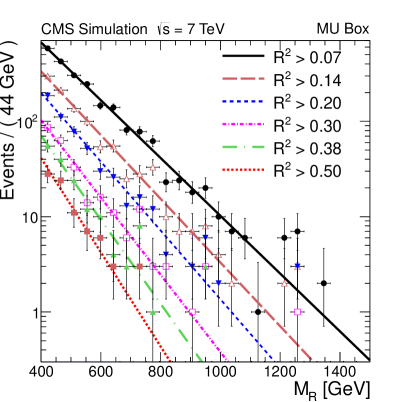
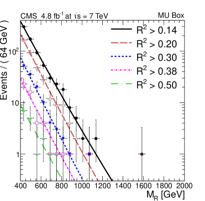
We perform an unbinned fit of the +jets distribution in simulated events passing the MU box selections with 2b-tagged events, using the sum of two separate exponential terms, as shown in Eq. (5). The fit allows us to obtain a parametric description of the background that is later used in the derivation of the remaining backgrounds, and it also permits the extrapolation of the prediction into the region of higher and values. The fit is performed in the region \GeVand is binned in values of as shown in Fig. 1. The fit to the simulated data, which provides a good description of the distribution, is used as the PDF to estimate the +b jets background in the signal box.
0.6.2 +jets background estimation
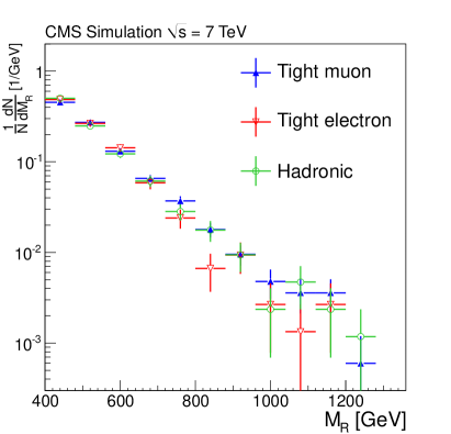
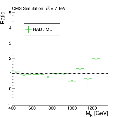
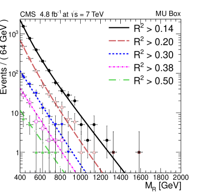
We estimate the background from the MU box, using 2b-tagged events in collision data (Section 0.4.2) and requiring the presence of a muon passing the tight identification requirements (Section 0.4.1). Based on comparisons with the MC simulation, approximately 90% of the events in this sample are . We find empirically from MC simulation studies that the shape of the distribution in both the tightly selected MU box and in the HAD box is very similar, as can be seen in Fig. 2. We therefore use the shape derived from the 2b-tagged sample to predict the background in the signal region. Additionally, because of a non-negligible contribution of +HF events in this sample, the imperfections in the background modeling in the simulation are absorbed into the background prediction. In order to derive the shape, we constrain the shape to that obtained from the MC simulation (Section 0.6.1). We find that a two-exponential function provides a good fit to the observed data in the MU box, as shown in Fig. 3.
0.6.3 Multijet background
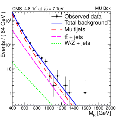
The remaining backgrounds that contribute significantly to the interesting region of high originate from heavy-flavor enriched multijet production. We use events with a loose muon in the MU box to derive the multijets background PDF. According to the MC simulation, this sample is composed 45% of top events, 5% of +b jet events, and 50% of multijet events.
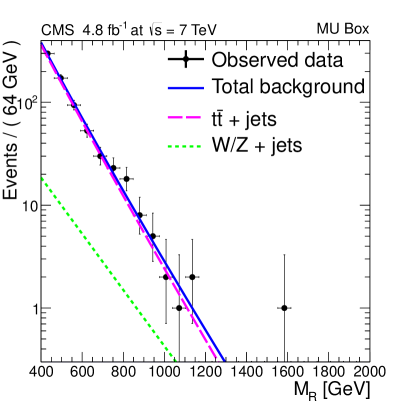
We proceed to perform the fits, for which the contributions from +b jets and backgrounds are fixed to the PDFs described in Sections 0.6.1 and 0.6.2. Based on simulation studies it is found that the parameters of the second component in the fit function ( and in Eq. (5)) are nearly idenical for the multijet and the +jets background processes. In order to better constrain the multijet fit, the parameters of the second component are set equal to those from the observed events for +jets while the parameters of the first component of the multijet PDF are left free. The results of the fit in the 2b-tagged MU box are displayed in Fig. 4, where we find good agreement between the fit results and observed data.
0.6.4 Systematic uncertainties
For the backgrounds estimated from observed events, the uncertainty in the total yield arises from the uncertainties (statistical and systematic) in the fit parameters in Eq. (5). We estimate these uncertainties by varying the threshold values (by %), thus arriving at a new set of and parameters describing the background PDF. The maximum difference observed between the experimental data and the simulated data in the MU box with tight and loose muon selections is then used as the uncertainty on the shape parameters. This procedure results in a 10% uncertainty in the values, and 40% in the values. We also tested the stability of the fits by varying the initial parameters used to start the fit by %, and found that this variation results in stable solutions, returning the same central value for the and parameters.
We generate an ensemble of pseudoexperiments, based on the fit results in the MU box. From each pseudoexperiment a new set of values for the parameters is then obtained, with the corresponding uncertainties, and we use the associated PDF results to predict the background yield. The ensemble of pseudoexperiments thus provides a distribution of the expected background yield in the signal regions, with its corresponding uncertainty. This procedure allows us to correctly propagate the systematic uncertainty in the background shape into the prediction of the background. To account for the normalization uncertainty we propagate the uncertainty in the introduced in Section 0.5 to the prediction of background yields in the signal region from control samples in observed events.
The effect of the jet energy scale (JES) and jet energy resolution (JER) uncertainties on the +jets background estimate and the signal model yields from simulation are taken into account. These effects are evaluated by repeating the extraction of all background PDFs by first varying the JES/JER by plus or minus one standard deviation in the +jet background model, and recalculating the and . These variations correspond to uncertainties as large as 3% in the selection efficiency. We then re-derive the background model PDFs from observed data in the MU box, using the newly obtained +HF jets model. The new set of PDFs with their corresponding covariance matrices then serve as an alternative background model.
We apply a scale factor of about 0.95, that is weakly dependent on jet , to account for an observed difference in tagging efficiency between data and simulation. The uncertainty in the scale factor varies from 0.03 to 0.05 for jets with from 30 to 670\GeV, and is 0.10 for b jets with . These uncertainties are measured using a dijet sample with high b-jet purity, as detailed in Ref. [CMS-PAS-BTV-11-004].
The uncertainty in the acceptance due to uncertainties in the parton distribution functions is calculated using the recommendation from the PDF4LHC group [Botje:2011sn]. The parton distribution function and the variations of next-to-leading (NLO) order in the MSTW2008 [Martin:2009iq], CTEQ6.6 [Nadolsky:2008zw], and NNPDF2.0 [Ball:2010de] sets were taken into account and their impact on the signal cross sections was compared with the calculation with CTEQ6L1 [PDFLQ3] that was used in the simulation of the signal samples. From these three sets we evaluate an upper and lower bound on the signal efficiency for each pair of assumed and \PSGczDo masses, and half of the difference between the two bounds is used as an estimate of the uncertainty. The theoretical cross section of LQ production has been calculated using CTEQ6L1 and CTEQ6M [PDFLQ3] at NLO, and the uncertainty in the prediction of the cross section was estimated by repeating the calculation using the NLO MRST2002 parametrization [Martin:2002aw]. This uncertainty was found to vary from 3.5 to 25% for leptoquarks in the mass range considered in this analysis [Kramer:2004df].
The systematic uncertainty to the luminosity measurement is taken to be 2.2% [CMS-PAS-SMP-12-008], which is correlated among all signal channels and the background estimates that are derived from simulations. The uncertainty in trigger efficiency is estimated using a set of prescaled razor triggers with low thresholds, and is found to be 2% for events in the HAD box, and 3% for events in the MU and ELE boxes.
0.6.5 ELE control region
In order to check that our background shape modeling indeed predicts the observed data adequately, we use the PDFs obtained in the steps described above (Sections 0.6.1-0.6.3) in an orthogonal sample in the 2b-tagged ELE box with a tight electron selection, i.e. the sample with a well-identified electron, which is then treated as a neutrino. This signal-depleted sample provides an independent cross-check of our background modeling, and covers the same region in and as the HAD box. Additionally, based on MC simulation studies, the composition of the tight ELE sample in observed events is similar to that of the HAD sample, consisting of approximately 85% , 5% +HF jets, and 10% multijet events. For comparison, the HAD sample is expected to contain approximately 70%, 5%, and 25% of the respective backgrounds.
Using the background model PDFs obtained from the fits, we derive the distribution of the expected shapes in the ELE box using pseudoexperiments. In order to correctly account for correlations and uncertainties in the parameters describing the background model, the shape parameters used to generate each pseudoexperiment data set are sampled from the covariance matrix returned by the fit. The actual number of events in each dataset is then drawn from a Poisson distribution centered on the yield returned by the covariance-matrix sampling. For each pseudoexperiment dataset, the number of events in the sideband and in the high- region is found. We then obtain the scale factor from the sideband region, which is used to predict the overall yield of background events in the high region of the ELE box.
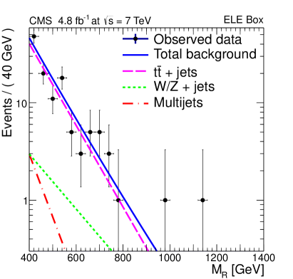
The comparison of the predicted distribution with the observed events in the ELE box is shown in Figure 5, and the background model is found to predict the observed data adequately. We also test our ability to correctly predict the yields of SM backgrounds using the scale factor mentioned above. The results are summarized in Table 0.6.5. Total background yield in the sideband is normalized to the number of observed data events in the sideband, in order to derive the scale factor , as described in Section 0.5. The uncertainties in the background yields shown here represent systematic uncertainties that are estimated by varying the parameters and , as described in Section 0.6.4. As can be seen in this comparison, the obtained from the sideband allows one to predict the overall normalization of the 2b-tagged sample.
Comparison of the yields in the ELE box. The sideband here refers to 2b-tagged events in the ELE box with \GeVand , while “signal-like” refers 2b-tagged events with \GeVand . The scale factor derived in the sideband () is used to normalize the background yield in the signal-like region (third column), and the uncertainty on the is propagated into the total background yield.
| Sideband | Signal-like | |
| Multijets | ||
| W/Z+jets | ||
| +jets | ||
| Other backgrounds | ||
| Total background | ||
| Observed data | 65 | 121 |
We perform another check to test whether the -dependence is well-described by our background model. This check is needed since in the final signal region we have several signal boxes, each optimized for different signal mass hypotheses. In order to increase the sensitivity for higher masses, a tighter selection on is imposed to reduce the backgrounds further, while keeping the signal efficiency high. In order to ensure that our background model adequately describes observed data with higher thresholds, we perform the same procedure in the ELE box. The results are summarized in Table 0.6.5. Here, we use the same derived from the sideband. As can be seen from these results, this model correctly predicts the total yields for higher boxes.
Expected and observed yields in the 2b-tagged ELE box for selections and a fixed requirement \GeV. The quoted uncertainties on the expected number of events include statistical and systematic uncertainties, and the uncertainty on the scale factor . Cut Expected yields Observed yields 121 0.25–0.30 48 0.30–0.35 26 0.35–0.38 11 0.38–0.42 11 25