KEK-TH-602, UT-828

hep-ph/9810479

October, 1998

Solar and Atmospheric Neutrino Oscillations
and
Lepton Flavor Violation
in
Supersymmetric Models with Right-handed Neutrinos

J. Hisano^(a) and Daisuke Nomura^(b)

$(a)$ Theory Group, KEK, Oho 1-1, Tsukuba, Ibaraki 305-0801, Japan

$(b)$ Department of Physics, University of Tokyo, Tokyo 113-0033, Japan

1 Introduction

Introduction of supersymmetry (SUSY) to the Standard Model (SM) is a solution for the naturalness problem on the radiative correction to the Higgs boson mass. The minimal supersymmetric standard model (MSSM) is considered as one of the most promising models beyond the Standard Model. Nowadays the signal of supersymmetry is being searched for by many experimental ways.

Lepton flavor conservation, lepton number conservation in each generation, is an exact symmetry in the SM, however, it may be violated in the MSSM [1]. The SUSY breaking mass terms for sleptons have to be introduced phenomenologically. Then, the mass eigenstates for sleptons may be different from those for leptons. This leads to the lepton flavor violating (LFV) rare processes, such as $\mu\to e\gamma$, $\tau\to\mu\gamma$, and so on. In fact, the experimental bounds on them have given a constraint on the slepton mass matrices.

The structure of the SUSY breaking mass matrices for sleptons depends on the mechanism to generate the SUSY breaking terms in the MSSM. One of the interesting mechanisms is the minimal supergravity (SUGRA) scenario. Similar to the slepton masses, arbitrary SUSY breaking masses for squarks are also strongly constrained from the FCNC processes, such as $K^{0}-\overline{K}^{0}$ mixing. In the minimal SUGRA scenario, the SUSY breaking masses for squarks, sleptons, and the Higgs bosons are expected to be given universally at the tree level, and we can escape from these phenomenological constraints.

However, the universality of the SUSY breaking masses for the scalar bosons is not stable for the radiative correction. Especially, if the physics below the gravitational scale $M_{\rm grav}$ ($\sim 10^{18}$GeV) has the LFV interaction, the interaction induces radiatively the LFV SUSY breaking masses for sleptons. Then, the LFV rare processes are sensitive to physics beyond the MSSM [2].

Recently, the Super-Kamiokande experiment has given us a convincing result [3] that the atmospheric neutrino anomaly [4] comes from the neutrino oscillation. From the zenith-angle dependence of $\nu_{e}$ and $\nu_{\mu}$ fluxes following neutrino mass square difference and mixing angle are expected,

$$\Delta m^{2}_{\nu_{\mu}\nu_{X}}\simeq(10^{-3}-10^{-2}){\rm eV^{2}},$$

$$\sin^{2}2\theta_{\nu_{\mu}\nu_{X}}\mathop{}_{\textstyle\sim}^{\textstyle>}0.8.$$ (1)

From the negative result for $\nu_{e}$-$\nu_{\mu}$ oscillation in the CHOOZ experiment [5] it is natural to consider $\nu_{X}=\nu_{\tau}$ from above results, and the tau neutrino mass is given as

$$m_{\nu_{\tau}}\simeq(3\times 10^{-2}-1\times 10^{-1}){\rm eV},$$ (2)

provided mass hierarchy $m_{\nu_{\tau}}\gg m_{\nu_{\mu}}$.

The simplest model to generate the neutrino masses is the seesaw mechanism [6]. The neutrino mass Eq. (2) leads to the right-handed neutrino masses below $\sim$ $(10^{14}-10^{15})$ GeV, even if the Yukawa coupling constant for the tau neutrino mass is of the order of one. This means that a LFV interaction exists below the gravitational scale. Then it is expected that the LFV large mixing for sleptons between the second- and the third-generations is generated radiatively in the minimal SUGRA scenario, and that the LFV rare processes may occur with rates accessible by future experiments [7, 8]. In fact, the branching ratio of $\tau\to\mu\gamma$ in the MSSM with the right-handed neutrinos can reach the present experimental bound [9].

The solar neutrino deficit [10] may also come from neutrino oscillation between $\nu_{\mu}$-$\nu_{e}$. The Mikheyev-Smirnov-Wolfenstein (MSW) solution [11] due to the matter effect in the sun is natural for its explanation, and the observation favors

$$\Delta m^{2}_{\nu_{e}\nu_{Y}}\simeq(8\times 10^{-6}-3\times 10^{-4}){\rm eV^{2}},$$

$$\sin^{2}2\theta_{\nu_{e}\nu_{Y}}\mathop{}_{\textstyle\sim}^{\textstyle>}0.5,$$ (3)

or

$$\Delta m^{2}_{\nu_{e}\nu_{Y}}\simeq(4\times 10^{-6}-1\times 10^{-5}){\rm eV^{2}},$$

$$\sin^{2}2\theta_{\nu_{e}\nu_{Y}}\simeq(10^{-3}-10^{-2}).$$ (4)

If the solar neutrino anomaly comes from so-called ’just so’ solution [12], neutrino oscillation in vacuum, the following mass square difference and mixing angle are expected [13],

$$\Delta m^{2}_{\nu_{e}\nu_{Y}}\simeq(6\times 10^{-11}-1\times 10^{-10}){\rm eV^{2}},$$

$$\sin^{2}2\theta_{\nu_{e}\nu_{Y}}\mathop{}_{\textstyle\sim}^{\textstyle>}0.5.$$ (5)

It is natural to consider $\nu_{Y}=\nu_{\mu}$, combined with the atmospheric neutrino observation. If one of the large angle solutions for the solar neutrino anomaly is true, the large mixing $\theta_{\nu_{\mu}\nu_{e}}$ may imply the LFV large mixing for sleptons between the first- and the second-generations.

In this article we investigate the LFV processes in the supersymmetric models with the right-handed neutrinos, assuming the minimal SUGRA scenario. We take the above results for the atmospheric and solar neutrinos. In section 2 after discussing the origin of the observed mixing angles we calculate the $\tau\to\mu\gamma$ and $\mu\to e\gamma$ branching ratios under the assumption of the MSSM with the right-handed neutrinos. It is argued that the $\mu\to e\gamma$ rate depends on the solar neutrino solutions, and that especially the MSW large angle solution naturally leads to a large $\mu\to e\gamma$ rate. In section 3 we consider them in the SU(5) SUSY GUT with the right-handed neutrinos. Here also it is shown that the large $\mu\to e\gamma$ rate naturally follows from the MSW large angle solution. Section 4 is for our conclusion. In Appendix A we give our convention used in this article. In Appendices B and C we show the multimass insertion formulas and their applications to $\tau\to\mu\gamma$ and $\mu\to e\gamma$, which are useful for estimating the LFV amplitudes and understanding the qualitative behavior of the LFV rates. In Appendix D the renormalization group equations (RGE’s) relevant for our discussion are given.

2 The Lepton Flavor Violation in the MSSM with Right-handed Neutrinos

Before starting to investigate the LFV rare processes in the MSSM with the right-handed neutrinos (MSSMRN), we discuss the origin of the large mixing of neutrino between $\nu_{\tau}$-$\nu_{\mu}$ or $\nu_{\mu}$-$\nu_{e}$. The MSSMRN is the simplest supersymmetric model to explain the neutrino masses, and following discussion is valid to the extension. The superpotential of the Higgs and lepton sector is given as

$$W_{\rm MSSMRN} = f_{\nu_{ij}}H_{2}\overline{N}_{i}L_{j}+f_{e_{ij}}H_{1}\overline{E}_{i}L_{j}+\frac{1}{2}M_{\nu_{i}\nu_{j}}\overline{N}_{i}\overline{N}_{j}+\mu H_{1}H_{2},$$ (6)

where $L$ is a chiral superfield for the left-handed lepton, and $\overline{N}$ and $\overline{E}$ are for the right-handed neutrino and the charged lepton. $H_{1}$ and $H_{2}$ are for the Higgs doublets in the MSSM. Here, $i$ and $j$ are generation indices. After redefinition of the fields, the Yukawa coupling constants and the Majorana masses can be taken as

$$f_{\nu_{ij}} = f_{\nu_{i}}V_{Dij},$$

$$f_{e_{ij}} = f_{e_{i}}\delta_{ij},$$

$$M_{\nu_{i}\nu_{j}} = U_{ik}^{\ast}M_{\nu_{k}}U^{\dagger}_{kj},$$ (7)

where $V_{D}$ and $U$ are unitary matrices. In this model the mass matrix for the left-handed neutrinos $(m_{\nu})$ becomes

$$(m_{\nu})_{ij} = V_{Dik}^{\top}(\overline{m}_{\nu})_{kl}V_{Dlj},$$ (8)

where

$$(\overline{m}_{\nu})_{ij} = m_{{\nu_{i}}D}\left[M^{-1}\right]_{ij}m_{{\nu_{j}}D}$$ (9)

$$\equiv V_{Mik}^{\top}m_{\nu_{k}}V_{Mkj}.$$

Here, $m_{{\nu_{i}}D}=f_{\nu_{i}}v\sin\beta/\sqrt{2}$ and $V_{M}$ is a unitary matrix. We assume $f_{\nu_{3}}\mathop{}_{\textstyle\sim}^{\textstyle>}f_{\nu_{2}}\mathop{}_{\textstyle\sim}^{\textstyle>}f_{\nu_{1}}$, similar to the quark sector, and $m_{\nu_{\tau}}\gg m_{\nu_{\mu}}\gg m_{\nu_{e}}$. Also, we take the Yukawa coupling and the Majorana masses for the right-handed neutrinos real for simplicity.

When we consider only the tau and the mu neutrino masses, we parameterize two unitary matrices as

$$V_{D}=\left(\begin{array}[]{cc}\cos\theta_{D}&\sin\theta_{D}\\ -\sin\theta_{D}&\cos\theta_{D}\end{array}\right), V_{M}=\left(\begin{array}[]{cc}\cos\theta_{M}&\sin\theta_{M}\\ -\sin\theta_{M}&\cos\theta_{M}\end{array}\right).$$ (14)

The observed large angle $\theta_{\nu_{\mu}\nu_{\tau}}$ is a sum of $\theta_{D}$ and $\theta_{M}$. However, in order to derive large $\theta_{M}$ we need to fine-tune the independent Yukawa coupling constants and the mass parameters. The neutrino mass matrix $(\overline{m}_{\nu})$ in the second and the third generations is written explicitly as

$$(\overline{m}_{\nu}) = \frac{1}{1-\frac{M_{\nu_{2}\nu_{3}}^{2}}{M_{\nu_{2}\nu_{2}}M_{\nu_{3}\nu_{3}}}}\left(\begin{array}[]{cc}\frac{m_{\nu_{2}D}^{2}}{M_{\nu_{2}\nu_{2}}}&-\frac{m_{\nu_{2}D}m_{\nu_{3}D}}{M_{\nu_{2}\nu_{3}}}\frac{M_{\nu_{2}\nu_{3}}^{2}}{M_{\nu_{2}\nu_{2}}M_{\nu_{3}\nu_{3}}}\\ -\frac{m_{\nu_{2}D}m_{\nu_{3}D}}{M_{\nu_{2}\nu_{3}}}\frac{M_{\nu_{2}\nu_{3}}^{2}}{M_{\nu_{2}\nu_{2}}M_{\nu_{3}\nu_{3}}}&\frac{m_{\nu_{3}D}^{2}}{M_{\nu_{3}\nu_{3}}}\end{array}\right).$$ (17)

If the following relations are imposed,

$$\frac{m_{\nu_{3}D}^{2}}{M_{\nu_{3}\nu_{3}}}\simeq\frac{m_{\nu_{2}D}^{2}}{M_{\nu_{2}\nu_{2}}}\simeq\frac{m_{\nu_{2}D}m_{\nu_{3}D}}{M_{\nu_{2}\nu_{3}}},$$ (18)

the neutrino mass hierarchy $m_{\nu_{\tau}}\gg m_{\nu_{\mu}}$ and $\theta_{M}\simeq\pi/4$ can be derived. However, it is difficult to explain the relation among the independent coupling constants and masses without some mechanism or symmetry. Also, the hierarchy $m_{\nu_{3}D}\gg m_{\nu_{2}D}$ suppresses the mixing angle $\theta_{M}$ as

$$\tan 2\theta_{M}\simeq 2\left(\frac{m_{\nu_{2}D}}{m_{\nu_{3}D}}\right)\left(\frac{M_{\nu_{2}\nu_{3}}}{M_{\nu_{2}\nu_{2}}}\right),$$ (19)

as far as the Majorana masses for the right-handed neutrinos do not have stringent hierarchical structure as Eq. (18). Therefore, in the following discussion we assume that the large mixing angle between $\nu_{\tau}$ and $\nu_{\mu}$ comes from $\theta_{D}$ and that $U$ is a unit matrix. Similarly, it is natural to consider that the large mixing angle between $\nu_{\mu}$ and $\nu_{e}$ in the MSW solution or the ’just so’ solution for the solar neutrino anomaly comes from $V_{D}$.

The existence of the large mixing angles in $V_{D}$ may lead to radiative generation of sizable LFV masses for the sleptons in the minimal SUGRA scenario. Though the SUSY breaking masses for the left-handed slepton are flavor-independent at tree level, the Yukawa interaction for the neutrino masses induces radiatively the LFV off-diagonal components in the left-handed slepton mass matrix.

The SUSY breaking terms for the Higgs and lepton sector in the MSSMRN are in general given as

$$-{\cal L}_{\rm\ SUSY\ breaking} = \phantom{+}(m_{\tilde{L}}^{2})_{ij}\tilde{l}_{Li}^{\dagger}\tilde{l}_{Lj}+(m_{\tilde{e}}^{2})_{ij}\tilde{e}_{Ri}^{\ast}\tilde{e}_{Rj}+(m_{\tilde{\nu}}^{2})_{ij}\tilde{\nu}_{Ri}^{\ast}\tilde{\nu}_{Rj}$$ (20)

$$+\tilde{m}_{h1}^{2}h_{1}^{\dagger}h_{1}+\tilde{m}_{h2}^{2}h_{2}^{\dagger}h_{2}$$

$$+(A_{\nu}^{ij}h_{2}\tilde{\nu}^{\ast}_{Ri}\tilde{l}_{Lj}+A_{e}^{ij}h_{1}\tilde{e}^{\ast}_{Ri}\tilde{l}_{Lj}+\frac{1}{2}B_{\nu}^{ij}\tilde{\nu}^{\ast}_{Ri}\tilde{\nu}^{\ast}_{Rj}+B_{h}h_{1}h_{2}+h.c.),$$

where $\tilde{l}_{L}$, $\tilde{e}_{R}$, and $\tilde{\nu}_{R}$ represent the left-handed slepton, and the right-handed charged slepton, and the right-handed sneutrino. Also, $h_{1}$ and $h_{2}$ are the doublet Higgs bosons. In the minimal SUGRA scenario at the gravitational scale the SUSY breaking masses for sleptons, squarks, and the Higgs bosons are universal, and the SUSY breaking parameters associated with the supersymmetric Yukawa couplings or masses (A or B parameters) are proportional to the Yukawa coupling constants or masses. Then, the SUSY breaking parameters in Eq. (20) are given as

$$(m_{\tilde{L}}^{2})_{ij}=(m_{\tilde{e}}^{2})_{ij}=(m_{\tilde{\nu}}^{2})_{ij}=\delta_{ij}m_{0}^{2},$$

$$\tilde{m}^{2}_{h1}=\tilde{m}^{2}_{h2}=m_{0}^{2},$$

$$A_{\nu}^{ij}=f_{\nu_{ij}}a_{0},~{}~{}~{}A_{e}^{ij}=f_{e_{ij}}a_{0},$$

$$B_{\nu}^{ij}=M_{\nu_{i}\nu_{j}}b_{0},~{}~{}~{}B_{h}=\mu b_{0}.$$ (21)

In order to know the values of the SUSY breaking parameters at the low energy, we have to include the radiative corrections to them. We can evaluate them by the RGE’s. We present them in Appendix D, and here we discuss only the qualitative behavior of the solution using the logarithmic approximation. The SUSY breaking masses of squarks, sleptons, and the Higgs bosons at the low energy are enhanced by gauge interactions, and the corrections are flavor-independent and proportional to square of the gaugino masses. On the other hand, Yukawa interactions reduce the SUSY breaking masses. If the Yukawa coupling is LFV, the radiative correction to the SUSY breaking parameters is LFV. The LFV off-diagonal components for $(m_{\tilde{L}}^{2})$, $(m_{\tilde{e}}^{2})$, and $A_{e}^{ij}$ are given at the low energy as

$$(m_{\tilde{L}}^{2})_{ij} \simeq -\frac{1}{8\pi^{2}}(3m_{0}^{2}+a_{0}^{2})V_{Dki}^{\ast}V_{Dkj}f_{\nu_{k}}^{2}\log\frac{M_{\rm grav}}{M_{\nu_{k}}},$$

$$(m^{2}_{\tilde{e}})_{ij} \simeq 0,$$

$$A_{e}^{ij} \simeq -\frac{3}{8\pi^{2}}a_{0}f_{e_{i}}V_{Dki}^{\ast}V_{Dkj}f_{\nu_{k}}^{2}\log\frac{M_{\rm grav}}{M_{\nu_{k}}},$$

where $i\neq j$. In these equations, the off-diagonal components of $(m_{\tilde{L}}^{2})$ and $A_{e}$ are generated radiatively while those of $(m_{\tilde{e}}^{2})$ are not. This is because the right-handed leptons have only one kind of the Yukawa interaction $f_{e}$ and we can always take a basis where $f_{e}$ is diagonal. The magnitudes of the off-diagonal components of $(m_{\tilde{L}}^{2})$ and $A_{e}$ are sensitive to $f_{\nu_{i}}$ and $V_{D}$.

As shown above, $V_{D32}$ is expected to be of the order of one from the atmospheric neutrino observation. This leads to the non-vanishing $(m_{\tilde{L}}^{2})_{32}$ and $A_{e}^{32}$, which result in a finite $\tau\to\mu\gamma$ decay rate via diagrams involving them. The dominant contributions are proportional to

$$(m_{\tilde{L}}^{2})_{32} \simeq -\frac{1}{8\pi^{2}}(3m_{0}^{2}+a_{0}^{2})V_{D33}^{\ast}V_{D32}f_{\nu_{3}}^{2}\log\frac{M_{\rm grav}}{M_{\nu_{3}}}.$$ (23)

As will be shown, if $f_{\nu_{3}}$ is of the order of one, the branching ratio of $\tau\to\mu\gamma$ may reach the present experimental bound.

Moreover if $V_{D31}$ is finite, $(m_{\tilde{L}}^{2})_{31}$ and $(m_{\tilde{L}}^{2})_{21}$ are also large. They are approximately

$$(m_{\tilde{L}}^{2})_{31} \simeq -\frac{1}{8\pi^{2}}(3m_{0}^{2}+a_{0}^{2})V_{D33}^{\ast}V_{D31}f_{\nu_{3}}^{2}\log\frac{M_{\rm grav}}{M_{\nu_{3}}},$$

$$(m_{\tilde{L}}^{2})_{21} \simeq -\frac{1}{8\pi^{2}}(3m_{0}^{2}+a_{0}^{2})V_{D32}^{\ast}V_{D31}f_{\nu_{3}}^{2}\log\frac{M_{\rm grav}}{M_{\nu_{3}}}.$$ (24)

This fact implies a sizable $\mu\to e\gamma$ rate because the amplitudes proportional to $(m^{2}_{\tilde{L}})_{23}(m^{2}_{\tilde{L}})_{31}$ or $(m^{2}_{\tilde{L}})_{21}$ are dominant. When $V_{D21}$ is also of the order of one to explain the solar neutrino anomaly, an extra contribution to $(m_{\tilde{L}}^{2})_{21}$ has to be taken into account as

$$(m_{\tilde{L}}^{2})_{21}\simeq-\frac{1}{8\pi^{2}}(3m_{0}^{2}+a_{0}^{2})\left(V_{D32}^{\ast}V_{D31}f_{\nu_{3}}^{2}\log\frac{M_{\rm grav}}{M_{\nu_{3}}}+V_{D22}^{\ast}V_{D21}f_{\nu_{2}}^{2}\log\frac{M_{\rm grav}}{M_{\nu_{2}}}\right).$$ (25)

The experimental upper bound on the branching ratio of $\mu\to e\gamma$ is so severe that the predicted branching ratio may reach it even if $f_{\nu_{2}}$ is ${\cal O}(10^{-1})$.

2.1 The Branching Ratio of $\tau\to\mu\gamma$

Let us discuss the branching ratios of the LFV rare processes in the MSSMRN. First, $\tau\to\mu\gamma$. The amplitude of the $e_{i}^{+}\to e_{j}^{+}\gamma$ ($i>j$) takes a form

$$T=e\epsilon^{\alpha*}(q)\bar{v}_{i}(p)i\sigma_{\alpha\beta}q^{\beta}(A^{(ij)}_{L}P_{L}+A^{(ij)}_{R}P_{R})v_{j}(p-q),$$ (26)

where $p$ and $q$ are momenta of $e_{i}$ and photon, and the decay rate is given by

$$\Gamma(e_{i}\to e_{j}\gamma)=\frac{e^{2}}{16\pi}m_{e_{i}}^{3}(|A^{(ij)}_{L}|^{2}+|A^{(ij)}_{R}|^{2}).$$ (27)

Here, we neglect the mass of $e_{j}$. The amplitude is not invariant for the SU(2)_L and U(1)_Y symmetry and the chiral symmetry of leptons. Then the coefficients $A^{(ij)}_{L}$ and $A^{(ij)}_{R}$ are proportional to the charged lepton masses. Since in the MSSMRN the mismatch between the left-handed slepton and the charged lepton mass eigenstates is induced, $A^{(ij)}_{L}$ is much larger than $A^{(ij)}_{R}$ since $A^{(ij)}_{R}$ is suppressed by $m_{e_{j}}/m_{e_{i}}$ compared with $A^{(ij)}_{L}$. Also, when $\tan\beta(\equiv v_{2}/v_{1})$ is large, the contribution to $A^{(ij)}_{L}$ proportional to $f_{e_{i}}v_{2}(=-\sqrt{2}m_{e_{i}}\tan\beta)$ becomes dominant. In the MSSMRN, the dominant contribution to $\tau\to\mu\gamma$ is from the diagram of Figs. (1)(a) and (b) and its expression is

$$A_{L}^{(\tau\mu)} \simeq m_{\tau}\frac{\alpha_{2}}{4\pi}\mu M_{2}\tan\beta(m^{2}_{\tilde{L}})_{32}$$ (28)

$$\times D\left[D\left[\frac{1}{m^{2}}\left\{f_{c2}\left(\frac{M^{2}}{m^{2}}\right)-\frac{1}{4}f_{n2}\left(\frac{M^{2}}{m^{2}}\right)\right\};M^{2}\right](M_{2}^{2},\mu^{2});m^{2}\right](m^{2}_{\tilde{\nu}_{\mu}},m^{2}_{\tilde{\nu}_{\tau}}),$$

which comes from the SU(2)_L interaction. The functions $f_{n2}(x)$ and $f_{c2}(x)$ are defined in Appendix C and the operator $D[f(x);x](x_{1},x_{2})$ to a function $f(x)$ is defined by

$$D[f(x);x](x_{1},x_{2})\equiv\frac{1}{x_{1}-x_{2}}(f(x_{1})-f(x_{2})).$$ (29)

Here, for a demonstrational purpose, we take a limit where the SUSY breaking scale is much larger than the $W$ and $Z$ gauge boson masses and $\tan\beta\mathop{}_{\textstyle\sim}^{\textstyle>}1$. This equation can be derived from the mass-insertion formula represented in Appendix C. The LFV A term can not give a dominant contribution when $\tan\beta\mathop{}_{\textstyle\sim}^{\textstyle>}1$.

In Fig. (2) we show the branching ratio of $\tau\to\mu\gamma$ as a function of the left-handed selectron mass ($m_{\tilde{e}_{L}}$). Here, $m_{\nu_{\tau}}=0.07$eV, $V_{D33}=V_{D22}=-V_{D32}=V_{D23}=1/\sqrt{2}$, and we assume that $f_{\nu_{3}}$ is as large as the Yukawa coupling constant for the top quark at the gravitational scale. This corresponds to $M_{\nu_{3}}\sim 10^{14}$GeV. Also, we impose the radiative breaking condition of the SU(2)${}_{L}\times$U(1)_Y gauge symmetry with $\tan\beta=3,10,30$ and the Higgsino mass parameter $\mu$ positive. In our calculation we considered the experimental constraints from the negative results of the SUSY particle search. Though we do not assume the GUT’s, we take the wino mass ($M_{2}$) 130GeV and determine the other gaugino masses by the GUT relation for the gaugino masses. We use the formula for $\tau\to\mu\gamma$ in Ref. [9] for the numerical calculation.

The branching ratio is reduced where the left-handed selectron mass is comparable to the wino mass. This is because the slepton masses are almost determined by the radiative correction from the gaugino masses, and $m^{2}_{0}$, which $(m_{\tilde{L}}^{2})_{32}$ is proportional to, is negligible in the region. As mentioned above, the branching ratio is proportional to $\tan^{2}\beta$ (see Eq. (28)), and the line for $\tan\beta=30$ is close to the experimental bound, ${\rm Br}(\tau\to\mu\gamma)<3.0\times 10^{-6}$ [14].

In Fig. (3) we present the dependence of the branching ratio of $\tau\to\mu\gamma$ on $M_{\nu_{3}}$. Here, we take $m_{\tilde{e}_{L}}=170$GeV, and the other SUSY breaking parameters are the same as in Fig. (2). The branching ratio is proportional to $M_{\nu_{3}}^{2}$ since we fix $m_{\nu_{\tau}}=0.07$eV. If $10^{-8}$ can be reached in the future experiments, we can probe $M_{\nu_{3}}>10^{13}(10^{14})$GeV for $\tan\beta=30(3)$.

2.2 The Branching Ratio of $\mu\to e\gamma$

Next, we discuss $\mu\to e\gamma$ in the MSSMRN. The forms of the amplitude and the event rate are the same as those of $\tau\to\mu\gamma$ (Eqs. (26,27)). This process has two types of the contribution, depending on the structure of the Yukawa coupling for the neutrino masses. One is the diagrams where $(m_{\tilde{L}}^{2})_{21}$ or $A_{e}^{21}$ is inserted, and another is those that $(m_{\tilde{L}}^{2})_{32}$ or $A_{e}^{32}$ and $(m_{\tilde{L}}^{2})_{13}$ or $A_{e}^{13}$ are inserted. Then the dominant contributions (Figs. (4)(a)-(d)) are following,

$$A_{L}^{(\mu e)} = -m_{\mu}\frac{\alpha_{2}}{4\pi}M_{2}\mu\tan\beta$$ (30)

$$\times D\left[\left\{\phantom{-}\left[(m^{2}_{\tilde{L}})_{21}+\frac{(m^{2}_{\tilde{L}})_{23}(m^{2}_{\tilde{L}})_{31}}{m^{2}_{\tilde{\nu}}-m^{2}_{\tilde{\nu}_{\tau}}}\right]\frac{1}{m^{4}_{\tilde{\nu}}}\left\{g_{c2}\left(\frac{M^{2}}{m^{2}_{\tilde{\nu}}}\right)-\frac{1}{4}g_{n2}\left(\frac{M^{2}}{m^{2}_{\tilde{\nu}}}\right)\right\}\right.\right.$$

$$\phantom{\times D\left[\left\{\right.\right.}\left.\left.-\left[\frac{(m^{2}_{\tilde{L}})_{23}(m^{2}_{\tilde{L}})_{31}}{(m^{2}_{\tilde{\nu}}-m^{2}_{\tilde{\nu}_{\tau}})^{2}}\right]\frac{1}{m^{2}_{\tilde{\nu}_{\tau}}}\left\{f_{c2}\left(\frac{M^{2}}{m^{2}_{\tilde{\nu}_{\tau}}}\right)-\frac{1}{4}f_{n2}\left(\frac{M^{2}}{m^{2}_{\tilde{\nu}_{\tau}}}\right)\right\}\right\};M^{2}\right](M^{2}_{2},\mu^{2})$$

Here, we take a limit where the SUSY breaking scale is much larger than the $W$ and $Z$ gauge boson masses and $\tan\beta\mathop{}_{\textstyle\sim}^{\textstyle>}1$, again. We also assumed the mass degeneracy between the first- and the second-generation left-handed sleptons as

$$m^{2}_{\tilde{e}_{L}}=m^{2}_{\tilde{\mu}_{L}}=m^{2}_{\tilde{\nu}_{e}}=m^{2}_{\tilde{\nu}_{\mu}}\equiv m^{2}_{\tilde{\nu}}.$$ (31)

The functions $f_{c2,n2}(x)$ and $g_{c2,n2}(x)$ are defined in Appendix C.

As mentioned above, if the solar neutrino anomaly comes from the MSW effect or the vacuum oscillation with the large angle, $V_{D21}$ is expected to be large. This leads to non-vanishing $(m_{\tilde{L}}^{2})_{21}$. In Fig. (5), under the condition that

$$V_{D}=\left(\begin{array}[]{ccc}0.91&0.35&0.24\\ -0.42&0.72&0.55\\ 0&-0.60&0.80\end{array}\right)$$ (32)

and $m_{\nu_{\mu}}=0.004$eV [17] we show the branching ratio of $\mu\to e\gamma$ as a function of $M_{\nu_{2}}$. This corresponds to the MSW solution with the large mixing. Here we take $V_{D31}=0$ and we will discuss a case with finite $V_{D31}$ later. The input parameters are taken to be the same as in Fig. (3). For $\tan\beta=30(3)$, the branching ratio reaches the experimental bound (${\rm Br}(\mu\to e\gamma)<4.9\times 10^{-11}$ [14]) when $M_{\nu_{2}}\simeq 8\times 10^{12}(8\times 10^{13})$GeV. This corresponds to $f_{\nu_{2}}\simeq 0.03(0.11)$. Future experiments are expected to reach 10^-14 [18]. This corresponds to $M_{\nu_{2}}\simeq 10^{11}$ $(10^{12})$GeV.

If the solar neutrino anomaly comes from the MSW solution with the small mixing, we cannot distinguish whether the mixing comes from $V_{D}$ or $V_{M}$. If it comes from $V_{D}$, the branching ratio is smaller by about 1/100 compared with that in the MSW solution with the large mixing, as shown in Fig. (6). In Fig. (6) we assume that

$$V_{D}=\left(\begin{array}[]{ccc}1&0.04&0.03\\ -0.04&0.79&0.59\\ 0&-0.60&0.80\end{array}\right)$$ (33)

and $m_{\nu_{\mu}}=0.0022$eV [17]. Other input parameters are the same as Fig. (5).

In Fig. (7) we take

$$V_{D}=\left(\begin{array}[]{ccc}\frac{1}{\sqrt{2}}&\frac{1}{2}&\frac{1}{2}\\ -\frac{1}{\sqrt{2}}&\frac{1}{2}&\frac{1}{2}\\ 0&-\frac{1}{\sqrt{2}}&\frac{1}{\sqrt{2}}\end{array}\right)$$ (34)

and $m_{\nu_{\mu}}=1.0\times 10^{-5}$eV [19]. Other parameters are the same as in Fig. (5). This corresponds to the ’just so’ solution for the solar neutrino anomaly. Since the mu neutrino mass is smaller, the branching ratio is suppressed by $10^{-5}$ compared with that in the MSW solution with the large mixing.

Next we discuss the branching ratio of $\mu\to e\gamma$ when $V_{D31}$ is finite. In Figs. (8,9) we show the branching ratio as a function of $V_{D31}$ and $M_{\nu_{3}}$ for $\tan\beta=3$ and 30. Here we assume that $f_{\nu_{2}}$ is negligibly small. The other parameters are the same as in Fig. (3). The branching ratio is almost proportional to $V_{D31}^{2}M_{\nu_{3}}^{2}$. Compared with this figure to Fig. (5), when $M_{\nu_{2}}=M_{\nu_{3}}$, the contribution from $V_{D31}$ is negligible in the MSW solution with the large mixing angle unless $V_{D31}$ is larger than $10^{-2.5}$. On the other hand, it can be dominant in the ’just so’ solution even if $V_{D31}\sim 10^{-4}$.

Finally we consider the $\mu^{+}\to e^{+}e^{-}e^{+}$ process and the $\mu$-$e$ conversion on ${}^{48}_{22}$Ti. For these processes the penguin type diagrams dominate over the others, so the behavior of the decay rate is similar to that of $\mu\to e\gamma$. For the $\mu\to 3e$ process the following approximate relation holds between the branching ratios of the two processes,

$${\rm Br}(\mu\to 3e) \simeq \frac{\alpha}{8\pi}\frac{8}{3}\left(\log\frac{m_{\mu}^{2}}{m_{e}^{2}}-\frac{11}{4}\right){\rm Br}(\mu\to e\gamma)$$ (35)

$$\simeq 7\times 10^{-3}{\rm Br}(\mu\to e\gamma).$$ (36)

For the $\mu$-$e$ conversion rate $\Gamma(\mu\to e)$ a similar relation holds at $\tan\beta>1$ region,

$$\Gamma(\mu\to e)\simeq 16\alpha^{4}Z_{\rm eff}^{4}Z|F(q^{2})|^{2}{\rm Br}(\mu\to e\gamma).$$ (37)

Here $Z$ is the proton number in the nucleus, and $Z_{\rm eff}$ is the effective charge, $F(q^{2})$ the nuclear form factor at the momentum transfer $q$. For ${}^{48}_{22}$Ti, $Z_{\rm eff}=17.6$ and $F(q^{2}\simeq-m_{\mu}^{2})\simeq 0.54$ [20, 21]. We express the magnitude of the $\mu$-$e$ conversion with the normalization the muon capture rate in Ti nucleus. Then the normalized conversion rate $R(\mu^{-}\to e^{-};{}^{48}_{22}{\rm Ti})$ is approximately

$$R(\mu^{-}\to e^{-};{}^{48}_{22}{\rm Ti})\simeq 6\times 10^{-3}{\rm Br}(\mu\to e\gamma).$$ (38)

The future experiment for the $\mu$-$e$ conversion is planed to reach $R(\mu^{-}\to e^{-};{}^{48}_{22}{\rm Ti})<10^{-18}$ [22].

3 The Lepton Flavor Violation in the SU(5) SUSY GUT with Right-handed Neutrinos

In the SUSY GUT the gauge coupling unification is predicted, and the predicted weak mixing angle is consistent with the experimental data at the 1 % level of accuracy. Moreover if the unified gauge group is SO(10), the right-handed neutrinos are introduced automatically into the matter multiplet. However, in order to accommodate the observed large mixing angle in the framework of the SO(10) SUSY GUT, one needs unnatural extension of the simplest version of the SO(10) SUSY GUT. Hence in this article we do not discuss the SO(10) SUSY GUT. Here we investigate the SU(5) SUSY GUT with the right-handed neutrinos as one of the extension of the MSSMRN in which the small neutrino mass is naturally obtained and the large neutrino mixing angle is possible without unnatural fine-tuning. We here call this model as SU(5)RN, for brevity. After introducing the model we estimate the off-diagonal elements of the slepton soft mass matrices using the one-loop level RGE’s under an assumption of the minimal SUGRA scenario. With them we study the LFV processes $\tau\to\mu\gamma$ and $\mu\to e\gamma$. After that we comment on the $b\to s\gamma$ branching ratio. We show that the LFV rates in this model is larger in general than those in the MSSMRN model, due to the fact that in this model the right-handed slepton mass matrix also can have non-negligible off-diagonal elements, in addition to the left-handed one [23, 24, 25].

First we introduce the model. This model has three families of matter multiplets $\psi_{i}$, $\phi_{i}$, and $\eta_{i}$, which are ${\bf 10}$, ${\bf 5}^{\ast}$, and ${\bf 1}$ dimension representations of SU(5), respectively. $\psi_{i}$ contains the quark doublet, the charged lepton singlet, and the up-type quark singlet, while $\phi_{i}$ the down-type quark singlet and the lepton doublet and $\eta_{i}$ the right-handed neutrino, respectively. The model has ${\bf 5}$ and ${\bf 5}^{\ast}$ dimension representation Higgs multiplets, $H$ and $\overline{H}$. $H$ consists of the MSSM Higgs multiplet $H_{2}$ and a colored Higgs multiplet $H_{C}$, and $\overline{H}$ another MSSM Higgs multiplet $H_{1}$ and another colored Higgs multiplet $\overline{H}_{C}$. The GUT gauge symmetry is spontaneously broken into the SM one at the GUT scale $M_{\rm GUT}\simeq 2\times 10^{16}$GeV. Above the GUT scale the superpotential $W$ of the matter sector of this model is

$$W = \frac{1}{4}f_{u_{ij}}\psi_{i}^{AB}\psi_{j}^{CD}H^{E}\epsilon_{ABCDE}+\sqrt{2}f_{d_{ij}}\psi_{i}^{AB}\phi_{jA}\overline{H}_{B}$$

$$+f_{\nu_{ij}}\eta_{i}\phi_{jA}H^{A}+\frac{1}{2}M_{\eta_{i}\eta_{j}}\eta_{i}\eta_{j},$$

where $A,B,...$ are indices of SU(5) and run from 1 to 5. We also introduce the soft SUSY breaking terms associated with the GUT multiplets. The relevant part of them is

$$-{\cal L}_{\rm SUSY~{}breaking} = (m_{\psi}^{2})_{ij}\tilde{\psi}_{i}^{\dagger}\tilde{\psi}_{j}+(m_{\phi}^{2})_{ij}\tilde{\phi}_{i}^{\dagger}\tilde{\phi}_{j}+(m_{\eta}^{2})_{ij}\tilde{\eta}_{i}^{\dagger}\tilde{\eta}_{j}+m_{h}^{2}h^{\dagger}h+m_{\bar{h}}^{2}\bar{h}^{\dagger}\bar{h}$$ (39)

$$+\left\{\frac{1}{4}A_{u_{ij}}\tilde{\psi}_{i}\tilde{\psi}_{j}h+\sqrt{2}A_{d_{ij}}\tilde{\psi}_{i}\tilde{\phi}_{j}\bar{h}+A_{\nu_{ij}}\tilde{\eta}_{i}\tilde{\phi}_{j}h+h.c.\right\},$$

where $\tilde{\psi}_{i}$, $\tilde{\phi}_{i}$, and $\tilde{\eta}_{i}$ are the scalar components of the ${\psi}_{i}$, ${\phi}_{i}$, and ${\eta}_{i}$ chiral multiplets, respectively, and $h$ and $\bar{h}$ are the Higgs bosons. In the minimal SUGRA scenario these coefficients are given at the gravitational scale as

$$(m_{\psi}^{2})_{ij}=(m_{\phi}^{2})_{ij}=(m_{\eta}^{2})_{ij}=\delta_{ij}m_{0}^{2},$$

$$m_{h}^{2}=m_{\bar{h}}^{2}=m_{0}^{2},$$

$$A_{u_{ij}}=f_{u_{ij}}a_{0},\,A_{d_{ij}}=f_{d_{ij}}a_{0},\,A_{\nu_{ij}}=f_{\nu_{ij}}a_{0}.$$ (40)

At the GUT scale we choose a basis where the up-type quark and the neutrino Yukawa coupling matrices are diagonalized as

$$f_{u_{ij}} = f_{u_{i}}e^{i\phi_{u_{i}}}\delta_{ij},$$

$$f_{d_{ij}} = (V^{\ast}_{\rm KM})_{ik}f_{d_{k}}(V_{D}^{\dagger})_{kj},$$

$$f_{\nu_{ij}} = f_{\nu_{i}}e^{i\phi_{\nu_{i}}}\delta_{ij},$$ (41)

where $f_{\psi_{i}}$ ($\psi=u,d,\nu$) are the eigenvalues of $f_{\psi_{ij}}$, respectively, $V_{\rm KM}$ the Kobayashi-Maskawa matrix at the GUT scale, and $V_{D}$ a unitary matrix which describes the generation mixing in the lepton sector. $\phi_{\psi_{i}}(\psi=u,\nu)$ are phase factors which satisfy $\phi_{u_{1}}+\phi_{u_{2}}+\phi_{u_{3}}=0$ and $\phi_{\nu_{1}}+\phi_{\nu_{2}}+\phi_{\nu_{3}}=0$. However these phases are completely irrelevant for our below discussion.

At the GUT scale the Yukawa coupling constants responsible to the down-type quark masses and those responsible to the charged lepton masses are supposed to unify as

$$f_{d_{i}}=f_{e_{i}}.$$ (42)

This relation is consistent with the particle spectrum at the low energy only for the third-generation. In order to explain the fermion masses of the first- and the second-generations, one has to consider the effect of the nonrenormalizable terms also. At that time those terms can be another source of LFV [26, 27], but we do not take them into account for simplicity.

Below the GUT scale we take the basis in which the Yukawa coupling constant matrix responsible for charged lepton masses is diagonalized. The basis we take at low energy region is related to that of GUT multiplets by the following embedding:

$$\psi_{i} = \{Q_{i},e^{-i\phi_{u_{i}}}\overline{U}_{i},(V_{\rm KM})_{ij}\overline{E}_{j}\},$$

$$\phi_{i} = \{V_{Dij}\overline{D}_{j},V_{Dij}L_{j}\},$$

$$\eta_{i} = \{e^{-i\phi_{\nu_{i}}}\overline{N}_{i}\}.$$ (43)

Then the superpotential $W$ is expanded in terms of the MSSM fields as

$$W = \phantom{+}f_{u_{i}}Q_{i}\overline{U}_{i}H_{2}+(V_{\rm KM}^{\ast})_{ij}f_{d_{j}}Q_{i}\overline{D}_{j}H_{1}$$ (44)

$$+f_{d_{i}}\overline{E}_{i}L_{i}H_{1}-f_{\nu_{i}}V_{Dij}\overline{N}_{i}L_{j}H_{2}$$

$$+f_{u_{j}}(V_{\rm KM})_{ji}\overline{E}_{i}\overline{U}_{j}H_{C}-\frac{1}{2}f_{u_{i}}e^{i\phi_{u_{i}}}Q_{i}Q_{i}H_{C}$$

$$+(V_{\rm KM}^{\ast})_{ij}f_{d_{j}}e^{-i\phi_{u_{i}}}\overline{U}_{i}\overline{D}_{j}\overline{H}_{C}-(V_{\rm KM}^{\ast})_{ij}f_{d_{j}}Q_{i}L_{j}\overline{H}_{C}$$

$$+f_{\nu_{i}}V_{Dij}\overline{N}_{i}\overline{D}_{j}H_{C}$$

$$+\frac{1}{2}M_{\nu_{i}\nu_{j}}\overline{N}_{i}\overline{N}_{j}.$$

Here we should notice that the fifth term of the right-hand side of the above equation is no longer generation-diagonal. This is nothing but a direct consequence of the GUT unification, that is, one of the central goal of the grand unification is to embed the leptons and the quarks into the same multiplet, which forces the mixing in the quark sector related to that of the lepton sector. No redefinition of $\overline{E}$ in generation-space can eliminate this mixing, as can be seen from Eq. (44). This mixing causes the off-diagonal elements of $(m^{2}_{\tilde{e}})$ via radiative corrections.

As for the origin of the observed mixing angle between the left-handed neutrinos a parallel discussion to that of the previous section applies. The Majorana mass matrix in Eq. (44) has an inter-generational mixing as

$$M_{\nu_{i}\nu_{j}}=U^{\ast}_{ik}M_{\nu_{k}}U^{\dagger}_{kj}.$$ (45)

The mass matrix of the left-handed neutrinos $(m_{\nu})$ is then

$$(m_{\nu})_{ij}=V^{\top}_{Dik}(\overline{m}_{\nu})_{kl}V_{Dlj},$$ (46)

where

$$(\overline{m}_{\nu})_{ij} = m_{{\nu_{i}}D}\left[M^{-1}\right]_{ij}m_{{\nu_{j}}D}$$ (47)

$$\equiv V_{Mik}^{\top}m_{\nu_{k}}V_{Mkj}.$$

Here also $m_{{\nu_{i}}D}=f_{\nu_{i}}v\sin\beta/\sqrt{2}$, the same notation as that of the previous section. The discussion in the previous section shows that the large mixing angle from $V_{M}$ requires a fine-tuning between the elements of $M_{\nu_{i}\nu_{j}}$ (Eq. (18)). Therefore as for the large mixing angle between neutrinos it is natural that its origin is in the mixing matrix $V_{D}$ in Eq. (44). Here we assume $U_{ij}=\delta_{ij}$, for simplicity, which means that the mixing comes only from $V_{D}$.

Now we evaluate the off-diagonal elements of the slepton mass matrices at the low energy. As stated above, both the left- and right-handed slepton’s ones have non-negligible off-diagonal elements at one-loop level. Assuming $m_{\nu_{e}}\ll m_{\nu_{\mu}}\ll m_{\nu_{\tau}}$ we neglect $f_{\nu_{1}}$, and also $f_{u_{1}}$ and $f_{u_{2}}$ to obtain approximate formulas for the off-diagonal elements of the slepton mass matrices as

$$(m^{2}_{\tilde{e}})_{ij} \simeq -\frac{3}{8\pi^{2}}f_{u_{3}}^{2}(V_{\rm KM})_{3i}(V^{\ast}_{\rm KM})_{3j}(3m_{0}^{2}+a_{0}^{2})\log\frac{M_{\rm grav}}{M_{\rm GUT}},$$ (48)

$$(m^{2}_{\tilde{L}})_{ij} \simeq -\frac{1}{8\pi^{2}}\left(f_{\nu_{3}}^{2}V^{\ast}_{D3i}V_{D3j}\log\frac{M_{\rm grav}}{M_{\nu_{3}}}+f_{\nu_{2}}^{2}V^{\ast}_{D2i}V_{D2j}\log\frac{M_{\rm grav}}{M_{\nu_{2}}}\right)(3m_{0}^{2}+a^{2}_{0}),$$ (49)

$$A_{e}^{ij} \simeq -\frac{3}{8\pi^{2}}a_{0}\left(f_{e_{i}}V_{D3i}^{\ast}V_{D3j}f_{\nu_{3}}^{2}\log\frac{M_{\rm grav}}{M_{\nu_{3}}}+f_{e_{i}}V_{D2i}^{\ast}V_{D2j}f_{\nu_{2}}^{2}\log\frac{M_{\rm grav}}{M_{\nu_{2}}}\right.$$ (50)

$$\phantom{-\frac{3}{8\pi^{2}}a_{0}}\left.+3f_{e_{j}}V_{{\rm KM}3j}^{\ast}V_{{\rm KM}3i}f_{u_{3}}^{2}\log\frac{M_{\rm grav}}{M_{\rm GUT}}\right),$$

for $i\neq j$. These formulas are obtained by a logarithmic approximation from the RGE’s (given in Appendix D).

Now we study the individual LFV processes. First we concentrate on the $\tau\to\mu\gamma$ decay. For $\tau\to\mu\gamma$ the most important contribution is from diagrams which involves $(m^{2}_{\tilde{L}})_{32}$ and winos (that is, diagrams of Figs. (10) (a) and (b)), which is the common feature with the MSSMRN case. These diagrams dominate because the large $V_{D32}$ element, suggested by the atmospheric neutrino anomaly, enhances $(m^{2}_{\tilde{L}})_{32}$ as

$$(m_{\tilde{L}}^{2})_{32}\simeq-\frac{1}{8\pi^{2}}(3m_{0}^{2}+a_{0}^{2})V_{D33}^{\ast}V_{D32}f_{\nu_{3}}^{2}\log\frac{M_{\rm grav}}{M_{\nu_{3}}},$$ (51)

which is the same situation as in the MSSMRN case. The main difference from the MSSMRN case is a presence of $(m_{\tilde{e}})_{32}$, but the contribution to the $\tau\to\mu\gamma$ is too small at the broad parameter region to be comparable to those from Figs. (10)(a) and (b), because $(m_{\tilde{e}})_{32}$ is suppressed by small $(V_{\rm KM})_{32}$ [28]. Our result of numerical calculation, Fig. (11), indeed shows that almost the same situation as in the MSSMRN case is realized. In the figure we plot the dependence of the branching ratio of $\tau\to\mu\gamma$ on the third generation right-handed Majorana mass $M_{\nu_{3}}$ for $\tan\beta=3$, 10, and 30. The upper curve corresponds to larger $\tan\beta$. We take the bino mass as 65GeV, the right-handed selectron mass 160GeV, and the tau neutrino mass 0.07eV, as expected from the atmospheric neutrino result. We take $a_{0}=0$ for simplicity. The figure shows us that the branching ratio of $\tau\to\mu\gamma$ is nearly proportional to the square of $M_{\nu_{3}}$. At the right-hand side of each curve the Yukawa coupling constant $f_{\nu_{3}}$ blows up below the gravitational scale, so the perturbative treatment is no longer valid in this region. In the region near $M_{\nu_{3}}\simeq 10^{14}$GeV the branching ratio is close to or even beyond the current experimental bound, ${\rm Br}(\tau\to\mu\gamma)<3.0\times 10^{-6}$ [14]. At relatively small $M_{\nu_{3}}$ region ($M_{\nu_{3}}\mathop{}_{\textstyle\sim}^{\textstyle<}4\times 10^{12}$GeV) the contribution from the right-handed slepton mass matrix (the diagrams shown in Figs. (10)(c) and (d)) tends to dominate, and the curves of the branching ratio show deviation from simple straight lines.

Next the $\mu\to e\gamma$ process. Since we know $V_{D32}={\cal O}(1)$ from the atmospheric neutrino result we can calculate $(m^{2}_{\tilde{L}})_{23}$ as

$$(m^{2}_{\tilde{L}})_{23}\simeq-\frac{1}{8\pi^{2}}f_{\nu_{3}}^{2}V^{\ast}_{D32}V_{D33}(3m^{2}_{0}+a^{2}_{0})\log\frac{M_{\rm grav}}{M_{\nu_{3}}}.$$ (52)

On the other hand $(m^{2}_{\tilde{e}})_{31}$ is determined from the GUT symmetry as

$$(m^{2}_{\tilde{e}})_{31}\simeq-\frac{3}{8\pi^{2}}f_{u_{3}}^{2}(V_{\rm KM})_{33}(V^{\ast}_{\rm KM})_{31}(3m^{2}_{0}+a^{2}_{0})\log\frac{M_{\rm grav}}{M_{\rm GUT}}.$$ (53)

Then we can definitely calculate the diagram shown in Fig. (12)(e), which contributes to $A^{(\mu e)}_{R}$ defined in Eq. (26). This contribution is proportional to $m_{\tau}$, and it tends to dominate over the other contribution to $A_{R}^{(\mu e)}$. We need to know $V_{D31}$ and $V_{D21}$ to calculate $A_{L}^{(\mu e)}$. However, we can evaluate only the lower bound of the branching ratio from the structure given in Eq. (27) even if we do not know them. The contribution from the diagram (e) can be so large that it reaches the present experimental bound at some parameter regions [28].

We can imagine some cases where much larger rate than this lower bound is predicted by the contribution from $A^{(\mu e)}_{L}$. One of such cases is that $V_{D31}$ is large. In this case, the diagrams in Figs. (12) (a)-(d) and (f) are enhanced since $(m^{2}_{\tilde{L}})_{31}$ and $(m^{2}_{\tilde{L}})_{21}$ are proportional to $V_{D31}$ as

$$(m^{2}_{\tilde{L}})_{31} \simeq -\frac{1}{8\pi^{2}}(3m_{0}^{2}+a_{0}^{2})f_{\nu_{3}}^{2}V^{\ast}_{D33}V_{D31}\log\frac{M_{\rm grav}}{M_{\nu_{3}}},$$ (54)

$$(m^{2}_{\tilde{L}})_{21} \simeq -\frac{1}{8\pi^{2}}(3m_{0}^{2}+a_{0}^{2})f_{\nu_{3}}^{2}V^{\ast}_{D32}V_{D31}\log\frac{M_{\rm grav}}{M_{\nu_{3}}}.$$ (55)

While the diagram (f) is enhanced by $m_{\tau}$, the contribution is suppressed by $(m_{\tilde{e}}^{2})_{32}$, which is proportional to $(V_{\rm KM})_{32}$. As a result, the diagrams (a)-(d) dominate since $V_{D32}$ is large. Also, if $f_{\nu_{2}}$ and $V_{D21}$ are non-negligibly large, $(m_{\tilde{e}}^{2})_{21}$ is enhanced as

$$(m^{2}_{\tilde{L}})_{21}\simeq-\frac{1}{8\pi^{2}}\left(f_{\nu_{3}}^{2}V^{\ast}_{D32}V_{D31}\log\frac{M_{\rm grav}}{M_{\nu_{3}}}+f_{\nu_{2}}^{2}V^{\ast}_{D22}V_{D21}\log\frac{M_{\rm grav}}{M_{\nu_{2}}}\right)(3m_{0}^{2}+a_{0}^{2}),$$ (56)

and the diagrams (a) and (c) dominate over the other contributions.

Now we examine these expectations numerically. First we set $f_{\nu_{2}}$ to zero and later investigate the non-zero $f_{\nu_{2}}$ case. We calculate the dependence of the branching ratio of $\mu\to e\gamma$ on $M_{\nu_{3}}$ and $V_{D31}$ in the Figs. (13, 14). In the figures we take $V_{D32}=-1/\sqrt{2}$ and the tau neutrino mass 0.07eV, as suggested by the atmospheric neutrino result. We neglect $m_{\nu_{\mu}}$ here. Other parameters are the bino mass 65GeV, the right-handed selectron mass 160GeV, $\tan\beta=3$ and 30, and the Higgsino mass $\mu>0$. From the Figs. (13,14) we can see that for $V_{D31}\mathop{}_{\textstyle\sim}^{\textstyle<}10^{-3}$ the diagram (e) dominates over the others. At relatively larger $V_{D31}$ region ($V_{D31}\mathop{}_{\textstyle\sim}^{\textstyle>}10^{-2.5}$) the diagrams (a)-(d) become dominant, and the predicted rate is large enough to reach the experimental bound for $V_{D31}\simeq 10^{-2}$ if $\tan\beta=30(3)$ and $M_{\nu_{3}}\mathop{}_{\textstyle\sim}^{\textstyle>}10^{13.5}(10^{14.5})$GeV.

Next let us consider the finite $f_{\nu_{2}}$ case. We show in Figs. (15, 16) the dependence of the $\mu\to e\gamma$ branching ratio on $V_{D31}$ and the typical right-handed neutrino Majorana mass $M_{N}$. In the figures the parameters that describe the MSW large angle solution are taken as the same as those we used in the MSSMRN case, and other parameters are taken as the same as in Figs. (13, 14). We assume in the figure the universality of the right-handed Majorana mass, that is, $M_{\nu_{1}}=M_{\nu_{2}}=M_{\nu_{3}}(\equiv M_{N})$. We can see from the figures that the enhancement due to the MSW large angle solution is so large that the dependence of the rate on $V_{D31}$ is small, and that the almost same situation as in the MSSMRN is reproduced here again, as can be seen when comparing these figures with Fig. (5). Since the dominant contribution is determined by the second term of Eq. (56), the rate is almost determined from the value of $M_{\nu_{2}}$ because $f^{2}_{\nu_{2}}\propto M_{\nu_{2}}$ for fixed $m_{\nu_{\mu}}$. Hence we can conclude from the Figs. (15,16) that for $\tan\beta=30(3)$ the excluded region of $M_{\nu_{2}}$ extends to $9\times 10^{12}(1\times 10^{14})$GeV, at least for the parameters chosen in our calculation.

We also calculated for the parameters suggested from the MSW small angle solution and the ’just so’ solution. For the MSW small angle solution the difference from the $f_{\nu_{2}}=0$ case is at most the factor 2 enhancement, and for the ’just so’ solution no difference from the $f_{\nu_{2}}=0$ case can be seen.

Finally we comment on the $b\to s\gamma$ process. This model has a characteristic feature that the right-handed neutrinos couple to the right-handed down-type quarks with the large mixing through the ninth term of Eq. (44). This coupling induces the off-diagonal elements in the right-handed down-type squark soft mass matrix via the radiative corrections, which are as large as

$$(m^{2}_{\tilde{d}_{R}})_{ij}\simeq-\frac{1}{8\pi^{2}}f_{\nu_{k}}^{2}V^{\ast}_{Dkj}V_{Dki}(3m_{0}^{2}+a_{0}^{2})\log\frac{M_{\rm grav}}{M_{\rm GUT}}.$$ (57)

This fact causes us an expectation that the $b\to s\gamma$ rate may become larger by the effect of the diagram which contains $(m^{2}_{\tilde{d}_{R}})_{23}$, by an exact analogy to that of the lepton sector. We examined whether this is true or not, and concluded that a tiny enhancement indeed occurs but it is too small to experimentally distinguishable. This is because the heavy gluino suppresses the contribution.

4 Conclusion

In this article taking the solar and the atmospheric neutrino experiment results into account we investigated the lepton flavor violating decay processes, such as $\mu\to e\gamma$ or $\tau\to\mu\gamma$ in the MSSM with the right-handed neutrinos (MSSMRN) and in the SU(5) SUSY GUT with the right-handed neutrinos (SU(5)RN).

In the MSSMRN we first studied the branching ratio of $\tau\to\mu\gamma$. It gets larger for larger $\tan\beta$ and almost proportional to $M_{\nu_{3}}^{2}$ for fixed $m_{\nu_{\tau}}$. A large rate naturally follows from the large mixing between $\nu_{\tau}$ and $\nu_{\mu}$, suggested by the atmospheric neutrino result. If $\tan\beta$=30(10) the rate reaches the current experimental bound for $M_{\nu_{3}}\sim 2\times 10^{14}(6\times 10^{14})$GeV. We investigated the $\mu\to e\gamma$ rate under three kinds of the solar neutrino solutions, the MSW large and small angle solutions and the ’just so’ solution. We argued that the $\mu\to e\gamma$ depends on $f_{\nu_{2}}$, and that especially the large $V_{D21}$ and the large $f_{\nu_{2}}$, which the MSW large angle solution suggests, naturally results in such a large rate that the predicted rate is beyond the current experimental bound if $M_{\nu_{2}}$ is larger than $8\times 10^{12}(8\times 10^{13})$GeV for $\tan\beta=30(3)$. We also investigated the dependence of $\mu\to e\gamma$ on $V_{D31}$. For $\tan\beta=30$ and $V_{D31}=10^{-2}$, $M_{\nu_{3}}\mathop{}_{\textstyle\sim}^{\textstyle>}3\times 10^{13}$GeV is excluded for our input parameters.

In the SU(5)RN we calculated the $\tau\to\mu\gamma$ rate. Here also the large mixing between $\nu_{\tau}$ and $\nu_{\mu}$ leads to a large rate, which is almost the same situation as in the MSSMRN. For $\mu\to e\gamma$ in this model, we can predict the lower bound of the branching ratio of it. This lower bound is calculable from the value of $m_{\nu_{\tau}}$ and the large mixing angle between $\nu_{\tau}$-$\nu_{\mu}$, suggested from the atmospheric neutrino result, and it turns out to be within accessible region by near future experiments. They are supposed to probe the $\mu\to e\gamma$ branching ratio to $10^{-14}$ level [18], and then the region $M_{\nu_{3}}>10^{13}(10^{12})$GeV can be probed for $\tan\beta=3(30)$ and $m_{\nu_{\tau}}=0.07$eV. We considered the relation between $\mu\to e\gamma$ and three kinds of the solar neutrino solutions. The large rate naturally follows from the MSW large angle solution, similarly to the MSSMRN case, while in the MSW small angle solution and in the ’just so’ solution there is only a little difference from the $f_{\nu_{2}}=0$ case.

If the LFV processes are discovered or the experimental bounds are improved by near future experiments, the interesting insight on the lepton sector will be obtained. The best effort to implement it is strongly desired.

Appendix A Definitions and Conventions in the MSSM

In this appendix we collect our notations of the MSSM used in our article. The superpotential of the MSSM $W_{\rm MSSM}$ is defined as

$$W_{\rm MSSM}\equiv f_{e_{ij}}H_{1}\overline{E}_{i}L_{j}+f_{d_{ij}}H_{1}Q_{i}\overline{D}_{j}+f_{u_{ij}}H_{2}Q_{i}\overline{U}_{j}+{\mu}H_{1}H_{2}.$$ (60)

We use $i$ and $j$ as the generation indices running from 1 to 3. $\overline{E},\overline{D}$, and $\overline{U}$ are the superfields associated with the right-handed electron $e_{R}$, the right-handed down-type quark $d_{R}$, and the right-handed up-type quark $u_{R}$, respectively. $Q$ and $L$ are ones associated with the quark doublet $q_{L}$ and the lepton doublet $l_{L}$ defined by

$$q_{L}=\left(\begin{array}[]{c}u_{L}\\ d_{L}\end{array}\right),\,\,l_{L}=\left(\begin{array}[]{c}\nu\\ e_{L}\end{array}\right),$$ (61)

and $H_{1}$ and $H_{2}$ the Higgs doublets whose SU(2)_L components we denote as

$$H_{1}=\left(\begin{array}[]{c}H^{0}_{1}\\ H^{-}_{1}\end{array}\right),\,\,H_{2}=\left(\begin{array}[]{c}H^{+}_{2}\\ H^{0}_{2}\end{array}\right).$$ (62)

The scalar components of $H_{1}^{0}$ and $H_{2}^{0}$ develop the vacuum expectation values (vev’s) as

$$\langle H_{1}^{0}\rangle\equiv\frac{v_{1}}{\sqrt{2}},\ \ \ \langle H_{2}^{0}\rangle\equiv\frac{v_{2}}{\sqrt{2}},$$ (63)

which satisfy $v_{1}^{2}+v_{2}^{2}=v^{2}$ with $v\simeq$ 246 GeV. We define the ratio of these vev’s as $\tan\beta$,

$$\tan\beta\equiv\frac{v_{2}}{v_{1}}.$$ (64)

The Yukawa couplings are given by the fermion masses and the Kobayashi-Maskawa matrix as

$$f_{e_{ij}} = -\sqrt{2}\frac{m_{e_{i}}}{v\cos\beta}\delta_{ij},$$

$$f_{d_{ij}} = -\sqrt{2}\frac{m_{d_{i}}}{v\cos\beta}\delta_{ij},$$

$$f_{u_{ij}} = \sqrt{2}\frac{m_{u_{i}}}{v\sin\beta}(V_{\rm KM})_{ij}.$$ (65)

We also introduce the soft SUSY breaking terms in the Lagrangian,

$$-{\cal L}_{\rm\ SUSY\ breaking} = \phantom{+}(m_{\tilde{L}}^{2})_{ij}\tilde{l}_{Li}^{\dagger}\tilde{l}_{Lj}+(m_{\tilde{e}}^{2})_{ij}\tilde{e}_{Ri}^{\ast}\tilde{e}_{Rj}$$ (66)

$$+(m_{\tilde{Q}}^{2})_{ij}\tilde{q}_{Li}^{\dagger}\tilde{q}_{Lj}+(m_{\tilde{u}}^{2})_{ij}\tilde{u}_{Ri}^{\ast}\tilde{u}_{Rj}+(m_{\tilde{d}}^{2})_{ij}\tilde{d}_{Ri}^{\ast}\tilde{d}_{Rj}$$

$$+\tilde{m}_{h1}^{2}h_{1}^{\dagger}h_{1}+\tilde{m}_{h2}^{2}h_{2}^{\dagger}h_{2}$$

$$+(A_{u}^{ij}h_{2}\tilde{q}_{Li}\tilde{u}^{\ast}_{Rj}+A_{d}^{ij}h_{1}\tilde{q}_{Li}\tilde{d}^{\ast}_{Rj}+A_{e}^{ij}h_{1}\tilde{e}^{\ast}_{Ri}\tilde{l}_{Lj}$$

$$\phantom{+}+B_{h}h_{1}h_{2}+h.c.)$$

$$+(\frac{1}{2}M_{1}\tilde{B}_{L}\tilde{B}_{L}+\frac{1}{2}M_{2}\tilde{W}^{a}_{L}\tilde{W}^{a}_{L}+\frac{1}{2}M_{3}\tilde{g}^{a}_{L}\tilde{g}^{a}_{L}+h.c.).$$

Here the first seven terms are the soft SUSY breaking masses for the doublet-slepton $\tilde{l}_{L}$, the right-handed charged slepton $\tilde{e}_{R}$, the doublet-squark $\tilde{q}_{L}$, the right-handed up-type (down-type) squark $\tilde{u}_{R}\ (\tilde{d}_{R})$, and the Higgs bosons. $\tilde{B}$, $\tilde{W}$, and $\tilde{g}$ stand for bino, wino, and gluino respectively, and the superscript $a$ is the gauge group index for each corresponding gauge group.

Now we discuss the slepton mass matrices. Let $\tilde{e}_{Li}$ and $\tilde{e}_{Ri}$ be the superpartners of the left-handed electron $e_{Li}$ and the right-handed electron $e_{Ri}$, respectively. Then the slepton mass matrix $(\overline{m}^{2}_{\tilde{e}})_{ij}$ is

$$-{\cal L}=\left(\tilde{e}_{Li}^{\dagger},\tilde{e}_{Ri}^{\dagger}\right)(\overline{m}^{2}_{\tilde{e}})_{ij}\left(\begin{array}[]{c}\tilde{e}_{Lj}\\ \tilde{e}_{Rj}\end{array}\right)\equiv\left(\tilde{e}_{Li}^{\dagger},\tilde{e}_{Ri}^{\dagger}\right)\left(\begin{array}[]{cc}(m^{2}_{L})_{ij}&(m^{2\top}_{LR})_{ij}\\ (m^{2}_{LR})_{ij}&(m^{2}_{R})_{ij}\end{array}\right)\left(\begin{array}[]{c}\tilde{e}_{Lj}\\ \tilde{e}_{Rj}\end{array}\right).$$ (67)

Here $m^{2}_{L}$ and $m^{2}_{R}$ are $3\times 3$ hermitian matrices and $m^{2}_{LR}$ is a $3\times 3$ matrix. They are given as

$$(m_{L}^{2})_{ij} = (m_{\tilde{L}}^{2})_{ij}+m_{e_{i}}^{2}\delta_{ij}+m_{Z}^{2}\delta_{ij}\cos 2\beta(-\frac{1}{2}+\sin^{2}\theta_{W}),$$ (68)

$$(m_{R}^{2})_{ij} = (m_{\tilde{e}}^{2})_{ij}+m_{e_{i}}^{2}\delta_{ij}-m_{Z}^{2}\delta_{ij}\cos 2\beta\sin^{2}\theta_{W},$$ (69)

$$(m_{LR}^{2})_{ij} = A^{ij}_{e}v\cos\beta/\sqrt{2}-m_{e_{i}}\mu\delta_{ij}\tan\beta.$$ (70)

As for the neutrinos we should notice that there is no right-handed sneutrino in the MSSM. Let $\tilde{\nu}_{i}$ be the superpartner of the left-handed neutrino $\nu_{i}$. The mass matrix of sneutrino $(\overline{m}^{2}_{\tilde{\nu}})_{ij}$ is

$$-{\cal L} = \tilde{\nu}^{\dagger}_{i}(\overline{m}^{2}_{\tilde{\nu}})_{ij}\tilde{\nu}_{j},$$

$$(\overline{m}^{2}_{\tilde{\nu}})_{ij} = (m_{\tilde{L}}^{2})_{ij}+\frac{1}{2}m_{Z}^{2}\delta_{ij}\cos 2\beta.$$ (71)

Next we discuss the mass matrix of gauginos. First we consider chargino mass matrix ${\cal M}_{C}$. It is a $2\times 2$ matrix that appears in the chargino mass terms,

$$-{\cal L}_{m}=\left(\overline{\tilde{W}^{-}_{R}}~{}\overline{\tilde{H}^{-}_{2R}}\right)\left(\begin{array}[]{cc}M_{2}&\sqrt{2}m_{W}\cos\beta\\ \sqrt{2}m_{W}\sin\beta&\mu\end{array}\right)\left(\begin{array}[]{c}\tilde{W}^{-}_{L}\\ \tilde{H}_{1L}^{-}\end{array}\right)+h.c..$$ (72)

${\cal M}_{C}$ is diagonalized by $2\times 2$ real orthogonal matrices $O_{L}$ and $O_{R}$ as

$$O_{R}{\cal M}_{C}O_{L}^{\top}={\rm diag}(M_{\tilde{\chi}_{1}^{-}},M_{\tilde{\chi}_{2}^{-}}).$$ (73)

Define the mass eigenstates $\tilde{\chi}_{AL(R)}$ $(A=1,2)$ by

$$\left(\begin{array}[]{c}\tilde{\chi}^{-}_{1L}\\ \tilde{\chi}^{-}_{2L}\end{array}\right)=O_{L}\left(\begin{array}[]{c}\tilde{W}^{-}_{L}\\ \tilde{H}^{-}_{1L}\end{array}\right),\hskip 42.67912pt\left(\begin{array}[]{c}\tilde{\chi}^{-}_{1R}\\ \tilde{\chi}^{-}_{2R}\end{array}\right)=O_{R}\left(\begin{array}[]{c}\tilde{W}^{-}_{R}\\ \tilde{H}^{-}_{2R}\end{array}\right).$$ (74)

Then

$$\tilde{\chi}^{-}_{A}=\tilde{\chi}^{-}_{AL}+\tilde{\chi}^{-}_{AR}\hskip 42.67912pt(A=1,2)$$ (75)

forms a Dirac fermion with mass $M_{\tilde{\chi}^{-}_{A}}$.

Finally we consider neutralinos. The mass matrix of the neutralino sector is given by

$$-{\cal L}_{m}=\frac{1}{2}\left(\tilde{B}_{L}\tilde{W}^{0}_{L}\tilde{H}^{0}_{1L}\tilde{H}^{0}_{2L}\right){\cal M}_{N}\left(\begin{array}[]{c}\tilde{B}_{L}\\ \tilde{W}^{0}_{L}\\ \tilde{H}^{0}_{1L}\\ \tilde{H}^{0}_{2L}\end{array}\right)+h.c.,$$ (76)

where

$${\cal M}_{N}=\left(\begin{array}[]{cccc}M_{1}&0&-m_{Z}\sin\theta_{W}\cos\beta&m_{Z}\sin\theta_{W}\sin\beta\\ 0&M_{2}&m_{Z}\cos\theta_{W}\cos\beta&-m_{Z}\cos\theta_{W}\sin\beta\\ -m_{Z}\sin\theta_{W}\cos\beta&m_{Z}\cos\theta_{W}\cos\beta&0&-\mu\\ m_{Z}\sin\theta_{W}\sin\beta&-m_{Z}\cos\theta_{W}\sin\beta&-\mu&0\end{array}\right).$$ (77)

The diagonalization is done by a real orthogonal matrix $O_{N}$,

$$O_{N}{\cal M}_{N}O_{N}^{\top}={\rm diag}(M_{\tilde{\chi}^{0}_{1}},...,M_{\tilde{\chi}^{0}_{4}}).$$ (78)

The mass eigenstates are given by

$$\tilde{\chi}^{0}_{AL}=(O_{N})_{AB}\tilde{X}^{0}_{BL}\hskip 42.67912pt(A,B=1,\cdots,4)$$ (79)

where

$$\tilde{X}^{0}_{AL}=(\tilde{B}_{L},\tilde{W}^{0}_{L},\tilde{H}^{0}_{1L},\tilde{H}^{0}_{2L}).$$ (80)

We have thus Majorana spinors

$$\tilde{\chi}^{0}_{A}=\tilde{\chi}^{0}_{AL}+\tilde{\chi}^{0}_{AR},{}~{}~{}~{}~{}(A=1,\cdots,4)$$ (81)

with mass $M_{\tilde{\chi}^{0}_{A}}$.

Now we give the interaction Lagrangian of lepton-slepton-chargino (-neutralino) in a basis of the slepton weak-eigenstate and the chargino (neutralino) mass-eigenstate. By writing the interactions in this basis we can get transparent view in the discussion of the multimass insertion technique discussed in Appendices B and C. The Lagrangian is

$$-{\cal L}_{\rm int} = \phantom{+}\tilde{\nu}_{i}^{\dagger}~{}\overline{\tilde{\chi}^{-}_{A}}(C^{A(i)}_{LR}P_{R}+C^{A(i)}_{LL}P_{L})~{}e_{i}$$ (82)

$$+\tilde{e}_{Li}^{\dagger}~{}\overline{\tilde{\chi}^{0}_{A}}(N^{A(i)}_{LR}P_{R}+N^{A(i)}_{LL}P_{L})~{}e_{i}$$

$$+\tilde{e}_{Ri}^{\dagger}~{}\overline{\tilde{\chi}^{0}_{A}}(N^{A(i)}_{RR}P_{R}+N^{A(i)}_{RL}P_{L})~{}e_{i}+h.c.,$$

where the coefficients are

$$C^{A(i)}_{LL} = g_{2}(O_{R})_{A1},$$

$$C^{A(i)}_{LR} = -\frac{\sqrt{2}m_{e_{i}}}{v\cos\beta}(O_{L})_{A2},$$

$$N^{A(i)}_{LL} = \frac{g_{2}}{\sqrt{2}}[-(O_{N})_{A2}-(O_{N})_{A1}\tan\theta_{W}],$$

$$N^{A(i)}_{RL} = \frac{\sqrt{2}m_{e_{i}}}{v\cos\beta}(O_{N})_{A3},$$

$$N^{A(i)}_{LR} = \frac{\sqrt{2}m_{e_{i}}}{v\cos\beta}(O_{N})_{A3},$$

$$N^{A(i)}_{RR} = \sqrt{2}g_{2}(O_{N})_{A1}\tan\theta_{W}.$$ (83)

Appendix B Multimass Insertion Technique

Mass insertion technique is useful to understand lepton flavor violating processes in the MSSM since only off-diagonal elements of the slepton mass matrices are sources of the flavor violation. In this appendix we introduce the multimass insertion technique with the nondegenerate masses. The multimass inserted diagrams may not be necessarily suppressed than the single-mass inserted ones when the slepton mass matrix has several small flavor-violating elements. Also, though in the previous mass insertion formulas the degeneracy of the slepton masses is sometimes assumed, such a degeneracy is not necessarily maintained at low energy even if the universal scalar mass hypothesis is assumed in the higher energy scale. Our rule to derive the mass-inserted amplitudes is very simple. We can derive them by taking the finite difference on amplitudes which have no mass-insertion. In this section we derive general formulas of $e^{+}_{i}\to e^{+}_{j}\gamma$ keeping in mind that we apply them to more realistic cases of $\mu^{+}\to e^{+}\gamma$ and $\tau^{+}\to\mu^{+}\gamma$ in the next section.

We refer to the slepton mass matrices as $(\overline{m}^{2}_{\tilde{l}})$,

$$-{\cal L}=\sum_{\tilde{l}=\tilde{e},\tilde{\nu}}(\overline{m}^{2}_{\tilde{l}})_{ij}\tilde{l}_{i}^{\dagger}\tilde{l}_{j}$$ (84)

where

$$\begin{array}[]{cclc}\tilde{e}_{i}&=&(\tilde{e}_{L},\tilde{\mu}_{L},\tilde{\tau}_{L},\tilde{e}_{R},\tilde{\mu}_{R},\tilde{\tau}_{R})^{\top}&({\rm for}~{}~{}\tilde{l}_{i}=\tilde{e}_{i}~{}~{}(i=1-6)),\\ \tilde{\nu}_{i}&=&(\tilde{\nu}_{e},\tilde{\nu}_{\mu},\tilde{\nu}_{\tau})^{\top}&({\rm for}~{}~{}\tilde{l}_{i}=\tilde{\nu}_{i}~{}~{}(i=1-3)).\end{array}$$ (85)

The explicit forms of these matrices are given in Appendix A. Here we assume that all the off-diagonal elements of the slepton mass matrices, both flavor violating and conserving ones, are much smaller than the diagonal elements, ($(\overline{m}^{2}_{\tilde{l}})_{ii}\gg(\overline{m}^{2}_{\tilde{l}})_{jk}$ ($j\neq k$)).

In the mass-insertion technique the internal slepton lines are classified to two types at one loop level. First type is a slepton line on which the momentum of slepton is not changed as

$$=\frac{1}{k^{2}-\overline{m}_{\tilde{l}_{1}}^{2}}(\overline{m}_{\tilde{l}}^{2})_{l_{1}l_{2}}\frac{1}{k^{2}-\overline{m}_{\tilde{l}_{2}}^{2}}(\overline{m}_{\tilde{l}}^{2})_{l_{2}l_{3}}\frac{1}{k^{2}-\overline{m}_{\tilde{l}_{3}}^{2}}(\overline{m}_{\tilde{l}}^{2})_{l_{3}l_{4}}\cdots(\overline{m}_{\tilde{l}}^{2})_{l_{N-1}l_{N}}\frac{1}{k^{2}-\overline{m}_{\tilde{l}_{N}}^{2}},$$ (86)

where we call the diagonal components of the slepton mass matrices, $(\overline{m}^{2}_{\tilde{l}})_{ii}$, as $\overline{m}^{2}_{\tilde{l}_{i}}$. We would like to consider the $e^{+}_{i}\to e^{+}_{j}\gamma$ process, and so in the above figure we mean that an anti-slepton is going from left to right with a momentum $k$. The product of propagators in above equation is referred to as $F_{N}$,

$$F_{N}(\overline{m}_{\tilde{l}_{1}}^{2},\overline{m}_{\tilde{l}_{2}}^{2},\cdots,\overline{m}_{\tilde{l}_{N}}^{2}) \equiv \frac{1}{k^{2}-\overline{m}_{\tilde{l}_{1}}^{2}}\frac{1}{k^{2}-\overline{m}_{\tilde{l}_{2}}^{2}}\cdots\frac{1}{k^{2}-\overline{m}_{\tilde{l}_{N}}^{2}}.$$ (87)

The second type is a slepton line where the momentum is changed, by an emission of a photon with an outgoing momentum $p$, as

$$= \frac{1}{(k+p)^{2}-\overline{m}_{l_{1}}^{2}}\frac{1}{k^{2}-\overline{m}_{l_{1}}^{2}}(\overline{m}_{\tilde{l}}^{2})_{l_{1}l_{2}}\frac{1}{k^{2}-\overline{m}_{l_{2}}^{2}}(\overline{m}_{\tilde{l}}^{2})_{l_{2}l_{3}}\cdots(\overline{m}_{\tilde{l}}^{2})_{l_{N-1}l_{N}}\frac{1}{k^{2}-\overline{m}_{l_{N}}^{2}}$$

$$+ \frac{1}{(k+p)^{2}-\overline{m}_{l_{1}}^{2}}(\overline{m}_{\tilde{l}}^{2})_{l_{1}l_{2}}\frac{1}{(k+p)^{2}-\overline{m}_{l_{2}}^{2}}\frac{1}{k^{2}-\overline{m}_{l_{2}}^{2}}(\overline{m}_{\tilde{l}}^{2})_{l_{2}l_{3}}\cdots(\overline{m}_{\tilde{l}}^{2})_{l_{N-1}l_{N}}\frac{1}{k^{2}-\overline{m}_{l_{N}}^{2}}$$

$$+ \cdots$$

$$+ \frac{1}{(k+p)^{2}-\overline{m}_{l_{1}}^{2}}(\overline{m}_{\tilde{l}}^{2})_{l_{1}l_{2}}\frac{1}{(k+p)^{2}-\overline{m}_{l_{2}}^{2}}(\overline{m}_{\tilde{l}}^{2})_{l_{2}l_{3}}\cdots(\overline{m}_{\tilde{l}}^{2})_{l_{N-1}l_{N}}\frac{1}{(k+p)^{2}-\overline{m}_{l_{N}}^{2}}\frac{1}{k^{2}-\overline{m}_{l_{N}}^{2}}.$$

The sum of product of propagators in this equation is referred to as $G_{N}$,

$$G_{N}(\overline{m}_{\tilde{l}_{1}}^{2},\overline{m}_{\tilde{l}_{2}}^{2},\cdots,\overline{m}_{\tilde{l}_{N}}^{2}) \equiv \frac{1}{(k+p)^{2}-\overline{m}_{\tilde{l}_{1}}^{2}}\frac{1}{k^{2}-\overline{m}_{\tilde{l}_{1}}^{2}}\frac{1}{k^{2}-\overline{m}_{\tilde{l}_{2}}^{2}}\cdots\frac{1}{k^{2}-\overline{m}_{\tilde{l}_{N}}^{2}}$$

$$+ \frac{1}{(k+p)^{2}-\overline{m}_{\tilde{l}_{1}}^{2}}\frac{1}{(k+p)^{2}-\overline{m}_{\tilde{l}_{2}}^{2}}\frac{1}{k^{2}-\overline{m}_{\tilde{l}_{2}}^{2}}\cdots\frac{1}{k^{2}-\overline{m}_{\tilde{l}_{N}}^{2}}$$

$$+ \cdots$$

$$+ \frac{1}{(k+p)^{2}-\overline{m}_{\tilde{l}_{1}}^{2}}\frac{1}{(k+p)^{2}-\overline{m}_{\tilde{l}_{2}}^{2}}\cdots\frac{1}{(k+p)^{2}-\overline{m}_{\tilde{l}_{N}}^{2}}\frac{1}{k^{2}-\overline{m}_{\tilde{l}_{N}}^{2}}.$$

These functions $F_{N}$ and $G_{N}$ can be given as a finite difference of $F_{N-1}$ and $G_{N-1}$,

$$F_{N}(\overline{m}_{\tilde{l}_{1}}^{2},\overline{m}_{\tilde{l}_{2}}^{2},\cdots,\overline{m}_{\tilde{l}_{N}}^{2}) = D[F_{N-1}(\overline{m}_{\tilde{l}}^{2},\overline{m}_{\tilde{l}_{3}}^{2},\cdots,\overline{m}_{\tilde{l}_{N}}^{2});\overline{m}_{\tilde{l}}^{2}](\overline{m}_{\tilde{l}_{1}}^{2},\overline{m}_{\tilde{l}_{2}}^{2}),$$ (90)

$$G_{N}(\overline{m}_{\tilde{l}_{1}}^{2},\overline{m}_{\tilde{l}_{2}}^{2},\cdots,\overline{m}_{\tilde{l}_{N}}^{2}) = D[G_{N-1}(\overline{m}_{\tilde{l}}^{2},\overline{m}_{\tilde{l}_{3}}^{2},\cdots,\overline{m}_{\tilde{l}_{N}}^{2});\overline{m}_{\tilde{l}}^{2}](\overline{m}_{\tilde{l}_{1}}^{2},\overline{m}_{\tilde{l}_{2}}^{2}),$$ (91)

where

$$D[f(x);x](x_{1},x_{2})\equiv\frac{1}{x_{1}-x_{2}}\left[f(x_{1})-f(x_{2})\right].$$ (92)

Then, by taking finite difference in sequence, each scalar line can be represented as a linear combination of flavor conserving scalar lines, $F_{1}$ or $G_{1}$,

$$F_{N}(\overline{m}_{\tilde{l}_{1}}^{2},\overline{m}_{\tilde{l}_{2}}^{2},\cdots,\overline{m}_{\tilde{l}_{N}}^{2}) = D^{N-1}[F_{1}(m^{2});m^{2}](\overline{m}_{\tilde{l}_{1}}^{2},\overline{m}_{\tilde{l}_{2}}^{2},\cdots,\overline{m}_{\tilde{l}_{N}}^{2}),$$

$$G_{N}(\overline{m}_{\tilde{l}_{1}}^{2},\overline{m}_{\tilde{l}_{2}}^{2},\cdots,\overline{m}_{\tilde{l}_{N}}^{2}) = D^{N-1}[G_{1}(m^{2});m^{2}](\overline{m}_{\tilde{l}_{1}}^{2},\overline{m}_{\tilde{l}_{2}}^{2},\cdots,\overline{m}_{\tilde{l}_{N}}^{2}),$$ (93)

where

$$D^{N-1}[f(x);x](x_{1},x_{2},\cdots,x_{N}) \equiv \sum^{N}_{i=1}\left(\prod_{j\neq i}\frac{1}{x_{i}-x_{j}}\right)f(x_{i}).$$ (94)

Due to this fact, we can get amplitudes with any masses inserted from the corresponding flavor-conserving diagrams.

Before we derive amplitudes of $e_{i}^{+}\to e_{j}^{+}\gamma$ $(i>j)$, we introduce a mass function $I_{N}^{M}$ as

$$iI_{N}^{M}(m_{1}^{2},m_{2}^{2},\cdots,m_{N}^{2}) = \int\frac{d^{4}k}{(\pi)^{2}}k^{2M}\prod_{i}^{N}\frac{1}{k^{2}-m_{i}^{2}}.$$ (95)

This function $I_{N}^{M}$ can be reduced to $I_{N-1}^{M}$ or $I_{N}^{M-1}$ by following rules,

$$I_{N}^{M}(m_{1}^{2},m_{2}^{2},\cdots,m_{N}^{2}) = D[I_{N-1}^{M}(m^{2},m_{3}^{2},\cdots,m_{N}^{2});m^{2}](m_{1}^{2},m_{2}^{2}),$$ (96)

$$I_{N}^{M}(m_{1}^{2},m_{2}^{2},\cdots,m_{N}^{2}) = m_{N}^{2}I_{N}^{M-1}(m_{1}^{2},m_{2}^{2},\cdots,m_{N}^{2})+I_{N-1}^{M-1}(m_{1}^{2},m_{2}^{2},\cdots,m_{N-1}^{2}),$$ (97)

and then, all $I_{N}^{M}$ for $N>2+M$ can be derived from $I_{1}^{0}$,

$$I^{0}_{1}(m^{2}) = \left(1-\log\frac{m^{2}}{\Lambda^{2}}\right)m^{2},$$ (98)

where $\Lambda$ is a renormalization point. Also, the signs of $I_{N}^{M}$ and $D^{L}[I_{N}^{M}]$ are definitely determined as

$$(-1)^{N+M}I_{N}^{M}(m_{1}^{2},m_{2}^{2},\cdots,m_{N}^{2})>0,$$ (99)

$$(-1)^{L+M+N}D^{L}[I_{N}^{M}(\underbrace{m^{2},m^{2},\cdots,m^{2}}_{N-P},m^{2}_{1},\cdots,m^{2}_{P});m^{2}](M^{2}_{1},M^{2}_{2},\cdots,M^{2}_{L+1})>0.$$ (100)

Then, we can discuss about relative signs between several diagrams definitely by using $I_{N}^{M}$ and the finite differences. Furthermore, since the mass dimension of $I_{N}^{M}$ is $(4+2M-2N)$, we can derive a following relation,

$$(2+M-N)I_{N}^{M}(m_{1}^{2},m_{2}^{2},\cdots,m_{N}^{2}) = \sum^{N}_{i=1}m_{i}^{2}I_{N+1}^{M}(m_{1}^{2},\cdots,m_{i}^{2},m_{i}^{2},\cdots,m_{N}^{2})$$ (101)

for $N>2+M$, since

$$\frac{d}{dx}\left\{x^{-2-M+N}I_{N}^{M}(xm_{1}^{2},xm_{2}^{2},\cdots,xm_{N}^{2})\right\} = 0.$$ (102)

Due to Eqs. (96,97,101) there are some ways to represent one function, for example,

$$I_{5}^{2}(m^{2},m^{2},m^{2},M^{2},M^{2}) = -3m^{2}I_{5}^{1}(m^{2},m^{2},m^{2},m^{2},M^{2}).$$ (103)

We will derive amplitudes of $e_{i}^{+}\to e_{j}^{+}\gamma$ $(i>j)$ by the mass-insertion technique. The amplitude is generally written as

$$T=e~{}\epsilon^{\alpha*}~{}\bar{v}_{i}(p)~{}i\sigma_{\alpha\beta}q^{\beta}~{}(A_{L}^{(ij)}P_{L}+A_{R}^{(ij)}P_{R})~{}v_{j}(p-q).$$ (104)

Here, $e$ is the electric charge, $\epsilon^{*}$ the photon polarization vector, $v_{i}$ and $v_{j}$ the wave functions for the external leptons. Assignment of momenta of the external fields is shown in Fig. (17). Since above term is violating the lepton chirality, it is convenient to decompose $A_{L}^{(ij)}$ and $A_{R}^{(ij)}$ as

$$A_{L}^{(ij)} = A^{(ij)}_{L}|_{c1}+A^{(ij)}_{L}|_{c2}+A^{(ij)}_{L}|_{n1}+A^{(ij)}_{L}|_{n2}+A^{(ij)}_{L}|_{n3},$$

$$A_{R}^{(ij)} = A^{(ij)}_{R}|_{c1}+A^{(ij)}_{R}|_{c2}+A^{(ij)}_{R}|_{n1}+A^{(ij)}_{R}|_{n2}+A^{(ij)}_{R}|_{n3}.$$ (105)

$A^{(ij)}_{L,R}|_{n1,c1}$ come from diagrams in which the lepton chirality is flipped on the external lines (Figs. (18)(a) and (b)). $A^{(ij)}_{L,R}|_{n2,c2}$ are contributions from the diagrams in which the chirality is flipped on a vertex of lepton-slepton-neutralino (-chargino) [Figs. (18)(c) and (d)]. $A^{(ij)}_{L,R}|_{n3}$ are contributions from those with the chirality flip on the internal slepton line (Fig. (18)(e)). Subscripts $c$ and $n$ represent that they are from chargino and neutralino diagrams, respectively.

The neutralino contribution to $A^{(ij)}_{L}|_{n1}$, derived from a diagram where the chirality of lepton is flipped in the external lepton line, is given by

$$A_{L}^{(ij)}|_{n1} = -\frac{1}{6(4\pi)^{2}}~{}m_{e_{i}}~{}N^{A(i)*}_{LL}N^{A(j)}_{LL}~{}\sum_{N=1}^{\infty}~{}\sum_{l_{1},\cdots,l_{N-1}}(\overline{m}_{\tilde{e}}^{2})_{l_{0}l_{1}}(\overline{m}_{\tilde{e}}^{2})_{l_{1}l_{2}}\cdots(\overline{m}_{\tilde{e}}^{2})_{l_{N-1}l_{N}}$$

$$\times D^{N}[I_{5}^{2}(\overline{m}^{2}_{\tilde{e}},\overline{m}^{2}_{\tilde{e}},\overline{m}^{2}_{\tilde{e}},M^{2}_{\tilde{\chi}^{0}_{A}},M^{2}_{\tilde{\chi}^{0}_{A}}),\overline{m}^{2}_{\tilde{e}}](\overline{m}^{2}_{\tilde{e}_{l_{0}}},\overline{m}^{2}_{\tilde{e}_{l_{1}}},\cdots,\overline{m}^{2}_{\tilde{e}_{l_{N}}})$$

$$~{}~{}~{}~{}~{}~{}~{}~{}~{}~{}~{}~{}~{}~{}~{}~{}~{}~{}(l_{0}=i,l_{N}=j),$$

$$A_{R}^{(ij)}|_{n1} = \left(A_{L}^{(ij)}|_{n1}\right)_{L\leftrightarrow R,l_{0}=i+3,l_{N}=j+3},$$ (106)

where $m_{e_{i}}$ is the $i$-th generation charged lepton mass, and the explicit form of $I_{5}^{1}$ is

$$I_{5}^{2}(\overline{m}^{2}_{\tilde{e}},\overline{m}^{2}_{\tilde{e}},\overline{m}^{2}_{\tilde{e}},M^{2}_{\tilde{\chi}^{0}},M^{2}_{\tilde{\chi}^{0}})=-\frac{1}{\overline{m}^{2}_{\tilde{e}}}\frac{1}{2(1-x)^{4}}(1-6x+3x^{2}+2x^{3}-6x^{2}\log x)$$ (107)

with $x=M^{2}_{\tilde{\chi}^{0}}/\overline{m}^{2}_{\tilde{e}}$. $N^{A(i)}_{LL}$ is a coupling constant between slepton and neutralino, and our definition of couplings of slepton to neutralino (or chargino) is

$$-{\cal L}_{\rm int} = ~{}~{}\tilde{\nu}_{i}^{\dagger}~{}\overline{\tilde{\chi}^{-}_{A}}(C^{A(i)}_{LR}P_{R}+C^{A(i)}_{LL}P_{L})~{}e_{i}$$ (108)

$$+\tilde{e}_{Li}^{\dagger}~{}\overline{\tilde{\chi}^{0}_{A}}(N^{A(i)}_{LR}P_{R}+N^{A(i)}_{LL}P_{L})~{}e_{i}$$

$$+\tilde{e}_{Ri}^{\dagger}~{}\overline{\tilde{\chi}^{0}_{A}}(N^{A(i)}_{RR}P_{R}+N^{A(i)}_{RL}P_{L})~{}e_{i}+h.c..$$

Here, $C^{A(i)}_{LL}$, $N^{A(i)}_{LL}$, and $N^{A(i)}_{RR}$ correspond to the (lepton-chirality conserving) gaugino interactions, and $C^{A(i)}_{LR}$, $N^{A(i)}_{RL}$, and $N^{A(i)}_{LR}$ are the (lepton-chirality violating) Higgsino interactions. These coupling constants are represented by the MSSM parameters in Appendix A.

Sign of the term with $N$ off-diagonal inserted-masses in $A_{L}^{(ij)}|_{n1}$ is definitely determined by signs of coupling constants of slepton to neutralino and the inserted masses, and is independent of the diagonal slepton masses and neutralino masses since

$$(-1)^{N+1}D^{N}[I_{5}^{2}(\overline{m}^{2}_{\tilde{e}},\overline{m}^{2}_{\tilde{e}},\overline{m}^{2}_{\tilde{e}},M^{2}_{\tilde{\chi}^{0}}M^{2}_{\tilde{\chi}^{0}}),\overline{m}^{2}_{\tilde{e}}](\overline{m}^{2}_{\tilde{e}_{0}},\overline{m}^{2}_{\tilde{e}_{1}},\cdots,\overline{m}^{2}_{\tilde{e}_{N}}) > 0.$$ (109)

A contribution from a neutralino diagram where the lepton chirality is flipped in the vertex of slepton-lepton-neutralino is given as

$$A_{L}^{(ij)}|_{n2} = -\frac{1}{2(4\pi)^{2}}~{}M_{\tilde{\chi}^{0}_{A}}~{}N^{A(i)*}_{LR}N^{A(j)}_{LL}~{}\sum_{N=1}^{\infty}~{}\sum_{l_{1},\cdots,l_{N-1}}(\overline{m}_{\tilde{e}}^{2})_{l_{0}l_{1}}(\overline{m}_{\tilde{e}}^{2})_{l_{1}l_{2}}\cdots(\overline{m}_{\tilde{e}}^{2})_{l_{N-1}l_{N}}$$

$$\times D^{N}[I_{4}^{1}(\overline{m}^{2}_{\tilde{e}},\overline{m}^{2}_{\tilde{e}},M^{2}_{\tilde{\chi}^{0}_{A}},M^{2}_{\tilde{\chi}^{0}_{A}});\overline{m}^{2}_{\tilde{e}}](\overline{m}^{2}_{\tilde{e}_{l_{0}}},\overline{m}^{2}_{\tilde{e}_{l_{1}}},\cdots,\overline{m}^{2}_{\tilde{e}_{l_{N}}})$$

$$~{}~{}~{}~{}~{}~{}~{}~{}~{}~{}~{}~{}~{}~{}~{}~{}~{}~{}(l_{0}=i,l_{N}=j),$$

$$A_{R}^{(ij)}|_{n2} = \left(A_{L}^{(ij)}|_{n2}\right)_{L\leftrightarrow R,l_{0}=i+3,l_{N}=j+3}.$$ (110)

The explicit form of $I_{4}^{1}$ in Eq. (110) is

$$I_{4}^{1}(\overline{m}^{2}_{\tilde{e}},\overline{m}^{2}_{\tilde{e}},M^{2}_{\tilde{\chi}^{0}},M^{2}_{\tilde{\chi}^{0}})=-\frac{1}{\overline{m}^{2}_{\tilde{e}}}\frac{1}{(1-x)^{3}}(1-x^{2}+2x\log x)$$ (111)

with $x=M^{2}_{\tilde{\chi}^{0}}/\overline{m}^{2}_{\tilde{e}}$, and the sign of $D^{N}[I_{4}^{1}]$ is $(-1)^{N+1}$ from Eq. (100).

A contribution from a neutralino diagram where the lepton chirality is flipped in the internal slepton line is given as

$$A_{L}^{(ij)}|_{n3} = -\frac{1}{2(4\pi)^{2}}~{}M_{\tilde{\chi}^{0}_{A}}~{}N^{A(i)*}_{RR}N^{A(j)}_{LL}~{}\sum_{N=1}^{\infty}~{}\sum_{l_{1},\cdots,l_{N-1}}(\overline{m}_{\tilde{e}}^{2})_{l_{0}l_{1}}(\overline{m}_{\tilde{e}}^{2})_{l_{1}l_{2}}\cdots(\overline{m}_{\tilde{e}}^{2})_{l_{N-1}l_{N}}$$

$$\times D^{N}[I_{4}^{1}(\overline{m}^{2}_{\tilde{e}},\overline{m}^{2}_{\tilde{e}},M^{2}_{\tilde{\chi}^{0}_{A}},M^{2}_{\tilde{\chi}^{0}_{A}});\overline{m}^{2}_{\tilde{e}}](\overline{m}^{2}_{\tilde{e}_{l_{0}}},\overline{m}^{2}_{\tilde{e}_{l_{1}}},\cdots,\overline{m}^{2}_{\tilde{e}_{l_{N}}})$$

$$~{}~{}~{}~{}~{}~{}~{}~{}~{}~{}~{}~{}~{}~{}~{}~{}~{}~{}(l_{0}=i+3,l_{N}=j),$$

$$A_{R}^{(ij)}|_{n3} = \left(A_{L}^{(ij)}|_{n3}\right)_{L\leftrightarrow R,l_{0}=i,l_{N}=j+3}.$$ (112)

A contribution from a chargino diagram where the lepton chirality is flipped in the external lepton line is given as

$$A_{L}^{(ij)}|_{c1} = \frac{1}{6(4\pi)^{2}}~{}m_{e_{i}}~{}C^{A(i)*}_{LL}C^{A(j)}_{LL}~{}\sum_{N=1}^{\infty}~{}\sum_{l_{1},\cdots,l_{N-1}}(\overline{m}_{\tilde{\nu}}^{2})_{l_{0}l_{1}}(\overline{m}_{\tilde{\nu}}^{2})_{l_{1}l_{2}}\cdots(\overline{m}_{\tilde{\nu}}^{2})_{l_{N-1}l_{N}}$$

$$\times D^{N}[I_{5}^{2}(\overline{m}^{2}_{\tilde{\nu}},\overline{m}^{2}_{\tilde{\nu}},M^{2}_{\tilde{\chi}^{-}_{A}},M^{2}_{\tilde{\chi}^{-}_{A}},M^{2}_{\tilde{\chi}^{-}_{A}});\overline{m}^{2}_{\tilde{\nu}}](\overline{m}^{2}_{\tilde{\nu}_{l_{0}}},\overline{m}^{2}_{\tilde{\nu}_{l_{1}}},\cdots,\overline{m}^{2}_{\tilde{\nu}_{l_{N}}})$$

$$~{}~{}~{}~{}~{}~{}(l_{0}=i,l_{N}=j),$$

$$A_{R}^{(ij)}|_{c1} = {\cal O}(m_{e_{j}}).$$ (113)

The explicit form of $I_{5}^{2}$ in Eq. (113) is

$$I_{5}^{2}(\overline{m}^{2}_{\tilde{\nu}},\overline{m}^{2}_{\tilde{\nu}},M^{2}_{\tilde{\chi}^{-}},M^{2}_{\tilde{\chi}^{-}},M^{2}_{\tilde{\chi}^{-}})=-\frac{1}{\overline{m}^{2}_{\tilde{\nu}}}\frac{1}{2(1-x)^{4}}(2+3x-6x^{2}+x^{3}+6x\log x)$$ (114)

with $x=M^{2}_{\tilde{\chi}^{-}}/\overline{m}^{2}_{\tilde{\nu}}$, and the sign of $D^{N}[I_{5}^{2}]$ is $(-1)^{N+1}$.

A contribution from a chargino diagram where the lepton chirality is flipped in the vertex of lepton-sneutrino-chargino is given as

$$A_{L}^{(ij)}|_{c2} = \frac{1}{(4\pi)^{2}}M_{\tilde{\chi}^{-}_{A}}C^{A(i)*}_{LR}C^{A(j)}_{LL}~{}\sum_{N=1}^{\infty}~{}\sum_{l_{1},\cdots,l_{N-1}}(\overline{m}_{\tilde{\nu}}^{2})_{l_{0}l_{1}}(\overline{m}_{\tilde{\nu}}^{2})_{l_{1}l_{2}}\cdots(\overline{m}_{\tilde{\nu}}^{2})_{l_{N-1}l_{N}}$$

$$\times D^{N}[I_{4}^{1}(\overline{m}^{2}_{\tilde{\nu}},M^{2}_{\tilde{\chi}^{-}_{A}},M^{2}_{\tilde{\chi}^{-}_{A}},M^{2}_{\tilde{\chi}^{-}_{A}});\overline{m}^{2}_{\tilde{\nu}}](\overline{m}^{2}_{\tilde{\nu}_{l_{0}}},\overline{m}^{2}_{\tilde{\nu}_{l_{1}}},\cdots,\overline{m}^{2}_{\tilde{\nu}_{l_{N}}})$$

$$~{}~{}~{}~{}~{}~{}(l_{0}=i,l_{N}=j),$$

$$A_{R}^{(ij)}|_{c2} = {\cal O}(m_{e_{j}}).$$ (115)

The explicit form of $I_{4}^{1}$ in Eq. (115) is

$$I_{4}^{1}(\overline{m}^{2}_{\tilde{\nu}},M^{2}_{\tilde{\chi}^{-}},M^{2}_{\tilde{\chi}^{-}},M^{2}_{\tilde{\chi}^{-}})=\frac{1}{\overline{m}^{2}_{\tilde{\nu}}}\frac{1}{2(1-x)^{3}}(3-4x+x^{2}+2\log x)$$ (116)

with $x=M^{2}_{\tilde{\chi}^{-}}/\overline{m}^{2}_{\tilde{\nu}}$, and the sign of $D^{N}[I_{4}^{1}]$ is $(-1)^{N+1}$.

Appendix C Application of Mass Insertion Formulas to $\tau^{+}\to\mu^{+}\gamma$ and $\mu^{+}\to e^{+}\gamma$

In this section we apply the formulas derived in the previous section to $\tau^{+}\to\mu^{+}\gamma$ and $\mu^{+}\to e^{+}\gamma$ processes. We neglect $m_{\mu}$ ($m_{e}$) in the calculation of $\tau^{+}\to\mu^{+}\gamma$ ($\mu^{+}\to e^{+}\gamma$). First we consider $\tau^{+}\to\mu^{+}\gamma$. The whole contribution to $\tau^{+}\to\mu^{+}\gamma$ can be written as

$$A_{L}^{(\tau\mu)} = A_{L}^{(\tau\mu)}|_{c1}+A_{L}^{(\tau\mu)}|_{c2}+A_{L}^{(\tau\mu)}|_{n1}+A_{L}^{(\tau\mu)}|_{n2}+A_{L}^{(\tau\mu)}|_{n3},$$

$$A_{R}^{(\tau\mu)} = A_{R}^{(\tau\mu)}|_{c1}+A_{R}^{(\tau\mu)}|_{c2}+A_{R}^{(\tau\mu)}|_{n1}+A_{R}^{(\tau\mu)}|_{n2}+A_{R}^{(\tau\mu)}|_{n3},$$ (117)

in the same notation as the previous section. In many models the dominant contributions to $\tau\to\mu\gamma$ are from the diagrams with single insertion of $(m_{\tilde{L}}^{2})_{32}$, $(m_{\tilde{e}}^{2})_{32}$, $A_{e}^{32}$, or $A_{e}^{23}$. Among these lepton flavor violating coupling constants only $(m_{\tilde{L}}^{2})_{32}$ and $(m_{\tilde{e}}^{2})_{32}$ are important for $\tan\beta\mathop{}_{\textstyle\sim}^{\textstyle>}1$. We here show explicit expressions of the diagrams with single off-diagonal slepton mass matrix element insertion for $\tan\beta\mathop{}_{\textstyle\sim}^{\textstyle>}1$. From the formula we derived in the previous Appendix, the contributions from diagrams with the lepton chirality flipped in the external line (Figs. (18)(a) and (b)) are given as

$$A_{L}^{(\tau\mu)}|_{c1} = -m_{\tau}\frac{1}{6}\frac{\alpha_{2}}{4\pi}(O_{R})_{A1}^{2}$$ (118)

$$\times\left[\frac{(m^{2}_{\tilde{L}})_{32}}{m_{\tilde{\nu}_{\mu}}^{2}-m_{\tilde{\nu}_{\tau}}^{2}}\right]~{}\left\{\frac{1}{m^{2}_{\tilde{\nu}_{\mu}}}f_{c1}(x_{A\tilde{\nu}_{\mu}})-\frac{1}{m^{2}_{\tilde{\nu}_{\tau}}}f_{c1}(x_{A\tilde{\nu}_{\tau}})\right\},$$

$$A_{R}^{(\tau\mu)}|_{c1} = {\cal O}(m_{\mu}),$$ (119)

$$A_{L}^{(\tau\mu)}|_{n1} = ~{}m_{\tau}\frac{1}{12}\frac{\alpha_{2}}{4\pi}~{}\left((O_{N})_{A2}+(O_{N})_{A1}\tan\theta_{W}\right)^{2}$$ (120)

$$\times\left[\frac{(m^{2}_{\tilde{L}})_{32}}{m_{\tilde{\mu}_{L}}^{2}-m_{\tilde{\tau}_{L}}^{2}}\right]~{}\left\{\frac{1}{m^{2}_{\tilde{\mu}_{L}}}f_{n1}(x_{A\tilde{\mu}_{L}})-\frac{1}{m^{2}_{\tilde{\tau}_{L}}}f_{n1}(x_{A\tilde{\tau}_{L}})\right\},$$

$$A_{R}^{(\tau\mu)}|_{n1} = ~{}m_{\tau}\frac{1}{3}\frac{\alpha_{Y}}{4\pi}~{}(O_{N})_{A1}^{2}$$ (121)

$$\times\left[\frac{(m^{2}_{\tilde{e}})_{32}}{m_{\tilde{\mu}_{R}}^{2}-m_{\tilde{\tau}_{R}}^{2}}\right]~{}\left\{\frac{1}{m^{2}_{\tilde{\mu}_{R}}}f_{n1}(x_{A\tilde{\mu}_{R}})-\frac{1}{m^{2}_{\tilde{\tau}_{R}}}f_{n1}(x_{A\tilde{\tau}_{R}})\right\},$$

where $x_{A\tilde{l}}=M^{2}_{\tilde{\chi}_{A}}/m^{2}_{\tilde{l}}$ with $l=\nu_{\mu}$, $\nu_{\tau}$, $\mu_{L}$, $\tau_{L}$, $\mu_{R}$, and $\tau_{R}$ and $\tilde{\chi}_{A}=\tilde{\chi}_{A}^{-}$ and $\tilde{\chi}_{A}^{0}$. The coefficient functions $f_{c1}(x)$ and $f_{n1}(x)$ are given as

$$f_{c1}(x) \equiv \frac{1}{2(1-x)^{4}}(2+3x-6x^{2}+x^{3}+6x\log x),$$ (122)

$$f_{n1}(x) \equiv \frac{1}{2(1-x)^{4}}(1-6x+3x^{2}+2x^{3}-6x^{2}\log x),$$ (123)

which are positive definite and monotonically decreasing. Following coefficient functions are also defined to be positive definite and monotonically decreasing.

The diagrams where the lepton chirality is flipped in the vertices give the following contributions,

$$A_{L}^{(\tau\mu)}|_{c2} = m_{\tau}\frac{\alpha_{2}}{4\pi}~{}\frac{M_{\tilde{\chi}_{A}^{-}}}{\sqrt{2}m_{W}\cos\beta}(O_{R})_{A1}(O_{L})_{A2}$$ (124)

$$\times\left[\frac{(m^{2}_{\tilde{L}})_{32}}{m_{\tilde{\nu}_{\mu}}^{2}-m_{\tilde{\nu}_{\tau}}^{2}}\right]\left\{\frac{1}{m^{2}_{\tilde{\nu}_{\mu}}}f_{c2}(x_{A\tilde{\nu}_{\mu}})-\frac{1}{m^{2}_{\tilde{\nu}_{\tau}}}f_{c2}(x_{A\tilde{\nu}_{\tau}})\right\},$$

$$A_{R}^{(\tau\mu)}|_{c2} = {\cal O}(m_{\mu}),$$ (125)

$$A_{L}^{(\tau\mu)}|_{n2} = -m_{\tau}\frac{1}{4}\frac{\alpha_{2}}{4\pi}\frac{M_{\tilde{\chi}_{A}^{0}}}{m_{Z}\cos\theta_{W}\cos\beta}(O_{N})_{A3}\left((O_{N})_{A2}+(O_{N})_{A1}\tan\theta_{W}\right)$$ (126)

$$\times\left[\frac{(m^{2}_{\tilde{L}})_{32}}{m_{\tilde{\mu}_{L}}^{2}-m_{\tilde{\tau}_{L}}^{2}}\right]\left\{\frac{1}{m^{2}_{\tilde{\mu}_{L}}}f_{n2}(x_{A\tilde{\mu}_{L}})-\frac{1}{m^{2}_{\tilde{\tau}_{L}}}f_{n2}(x_{A\tilde{\tau}_{L}})\right\},$$

$$A_{R}^{(\tau\mu)}|_{n2} = m_{\tau}\frac{1}{2}\frac{\alpha_{Y}}{4\pi}\frac{M_{\tilde{\chi}_{A}^{0}}}{m_{Z}\sin\theta_{W}\cos\beta}(O_{N})_{A3}(O_{N})_{A1}$$ (127)

$$\times\left[\frac{(m^{2}_{\tilde{e}})_{32}}{m_{\tilde{\mu}_{R}}^{2}-m_{\tilde{\tau}_{R}}^{2}}\right]\left\{\frac{1}{m^{2}_{\tilde{\mu}_{R}}}f_{n2}(x_{A\tilde{\mu}_{R}})-\frac{1}{m^{2}_{\tilde{\tau}_{R}}}f_{n2}(x_{A\tilde{\tau}_{R}})\right\},$$

where the functions $f_{c2}(x)$ and $f_{n2}(x)$ are defined as

$$f_{c2}(x) \equiv -\frac{1}{2(1-x)^{3}}(3-4x+x^{2}+2\log x),$$ (128)

$$f_{n2}(x) \equiv \frac{1}{(1-x)^{3}}(1-x^{2}+2x\log x).$$ (129)

Finally the contribution from the diagrams in which the lepton chirality is flipped on the internal slepton lines are

$$A_{L}^{(\tau\mu)}|_{n3} = -\frac{1}{2}\frac{\alpha_{2}}{4\pi}(O_{N})_{A1}\left((O_{N})_{A2}+(O_{N})_{A1}\tan\theta_{W}\right)\tan\theta_{W}(m^{2}_{LR})_{33}(m^{2}_{\tilde{L}})_{32}M_{\tilde{\chi}_{A}^{0}}$$ (130)

$$\times\left\{\phantom{+}\frac{1}{m^{2}_{\tilde{\tau}_{R}}}\frac{1}{m^{2}_{\tilde{\tau}_{R}}-m^{2}_{\tilde{\tau}_{L}}}\frac{1}{m^{2}_{\tilde{\tau}_{R}}-m^{2}_{\tilde{\mu}_{L}}}f_{n2}(x_{A\tilde{\tau}_{R}})\right.$$

$$\phantom{\times\left\{\right.}+\frac{1}{m^{2}_{\tilde{\tau}_{L}}}\frac{1}{m^{2}_{\tilde{\tau}_{L}}-m^{2}_{\tilde{\tau}_{R}}}\frac{1}{m^{2}_{\tilde{\tau}_{L}}-m^{2}_{\tilde{\mu}_{L}}}f_{n2}(x_{A\tilde{\tau}_{L}})$$

$$\phantom{\times\left\{\right.}\left.+\frac{1}{m^{2}_{\tilde{\mu}_{L}}}\frac{1}{m^{2}_{\tilde{\mu}_{L}}-m^{2}_{\tilde{\tau}_{R}}}\frac{1}{m^{2}_{\tilde{\mu}_{L}}-m^{2}_{\tilde{\tau}_{L}}}f_{n2}(x_{A\tilde{\mu}_{L}})\right\},$$

$$A_{R}^{(\tau\mu)}|_{n3} = -\frac{1}{2}\frac{\alpha_{2}}{4\pi}(O_{N})_{A1}\left((O_{N})_{A2}+(O_{N})_{A1}\tan\theta_{W}\right)\tan\theta_{W}(m^{2}_{LR})_{33}(m^{2}_{\tilde{e}})_{32}M_{\tilde{\chi}_{A}^{0}}$$ (131)

$$\times\left\{\phantom{+}\frac{1}{m^{2}_{\tilde{\tau}_{L}}}\frac{1}{m^{2}_{\tilde{\tau}_{L}}-m^{2}_{\tilde{\tau}_{R}}}\frac{1}{m^{2}_{\tilde{\tau}_{L}}-m^{2}_{\tilde{\mu}_{R}}}f_{n2}(x_{A\tilde{\tau}_{L}})\right.$$

$$\phantom{\times\left\{\right.}+\frac{1}{m^{2}_{\tilde{\tau}_{R}}}\frac{1}{m^{2}_{\tilde{\tau}_{R}}-m^{2}_{\tilde{\tau}_{L}}}\frac{1}{m^{2}_{\tilde{\tau}_{R}}-m^{2}_{\tilde{\mu}_{R}}}f_{n2}(x_{A\tilde{\tau}_{R}})$$

$$\phantom{\times\left\{\right.}\left.+\frac{1}{m^{2}_{\tilde{\mu}_{R}}}\frac{1}{m^{2}_{\tilde{\mu}_{R}}-m^{2}_{\tilde{\tau}_{L}}}\frac{1}{m^{2}_{\tilde{\mu}_{R}}-m^{2}_{\tilde{\tau}_{R}}}f_{n2}(x_{A\tilde{\mu}_{R}})\right\}.$$

Next we present the mass insertion formula for $\mu^{+}\to e^{+}\gamma$. Here we assume mass degeneracy between selectron and smuon, then

$$m_{\tilde{\nu}_{e}} = m_{\tilde{\nu}_{\mu}}~{}\equiv~{}~{}m_{\tilde{\nu}},$$

$$m_{\tilde{e}_{L}} = m_{\tilde{\mu}_{L}}~{}\equiv~{}~{}m_{\tilde{l}_{L}},$$

$$m_{\tilde{e}_{R}} = m_{\tilde{\mu}_{R}}~{}\equiv~{}~{}m_{\tilde{l}_{R}}.$$

The contributions from diagrams with the lepton chirality flipped in the external line (Figs. (18)(a) and (b)) are given as

$$A_{L}^{(\mu e)}|_{c1} = ~{}~{}~{}m_{\mu}\frac{1}{6}\frac{\alpha_{2}}{4\pi}(O_{R})^{2}_{A1}$$ (132)

$$\times\left\{\left[(m^{2}_{\tilde{L}})_{21}+\frac{(m^{2}_{\tilde{L}})_{23}(m^{2}_{\tilde{L}})_{31}}{m_{\tilde{\nu}}^{2}-m_{\tilde{\nu}_{\tau}}^{2}}\right]\frac{1}{m^{4}_{\tilde{\nu}}}g_{c1}(x_{A\tilde{\nu}})\right.$$

$$~{}~{}-~{}\left.\left[\frac{(m^{2}_{\tilde{L}})_{23}(m^{2}_{\tilde{L}})_{31}}{(m_{\tilde{\nu}}^{2}-m_{\tilde{\nu}_{\tau}}^{2})^{2}}\right]\frac{1}{m^{2}_{\tilde{\nu}_{\tau}}}f_{c1}(x_{A\tilde{\nu}_{\tau}})\right\},$$

$$A_{R}^{(\mu e)}|_{c1} = {\cal O}(m_{e}),$$ (133)

$$A_{L}^{(\mu e)}|_{n1} = -m_{\mu}\frac{1}{12}\frac{\alpha_{2}}{4\pi}\left((O_{N})_{A2}+(O_{N})_{A1}\tan\theta_{W}\right)^{2}$$ (134)

$$\times\left\{\left[(m^{2}_{\tilde{L}})_{21}+\frac{(m^{2}_{\tilde{L}})_{23}(m^{2}_{\tilde{L}})_{31}}{m_{\tilde{l}_{L}}^{2}-m_{\tilde{\tau}_{L}}^{2}}\right]\frac{1}{m^{4}_{\tilde{l}_{L}}}g_{n1}(x_{A\tilde{l}_{L}})\right.$$

$$~{}~{}-~{}\left.\left[\frac{(m^{2}_{\tilde{L}})_{23}(m^{2}_{\tilde{L}})_{31}}{(m_{\tilde{l}_{L}}^{2}-m_{\tilde{\tau}_{L}}^{2})^{2}}\right]\frac{1}{m^{2}_{\tilde{\tau}_{L}}}f_{n1}(x_{A\tilde{\tau}_{L}})\right\},$$

$$A_{R}^{(\mu e)}|_{n1} = ~{}-\frac{1}{3}m_{\mu}\frac{\alpha_{Y}}{4\pi}(O_{N})_{A1}^{2}$$ (135)

$$\times\left\{\left[(m^{2}_{\tilde{e}})_{21}+\frac{(m^{2}_{\tilde{e}})_{23}(m^{2}_{\tilde{e}})_{31}}{m_{\tilde{l}_{R}}^{2}-m_{\tilde{\tau}_{R}}^{2}}\right]~{}\frac{1}{m^{4}_{\tilde{l}_{R}}}g_{n1}(x_{A\tilde{l}_{R}})\right.$$

$$~{}~{}-~{}\left.\left[\frac{(m^{2}_{\tilde{e}})_{23}(m^{2}_{\tilde{e}})_{31}}{(m_{\tilde{l}_{R}}^{2}-m_{\tilde{\tau}_{R}}^{2})^{2}}\right]\frac{1}{m^{2}_{\tilde{\tau}_{R}}}f_{n1}(x_{A\tilde{\tau}_{R}})\right\},$$

with

$$g_{c1}(x) \equiv f_{c1}(x)+xf^{\prime}_{c1}(x),$$

$$g_{n1}(x) \equiv f_{n1}(x)+xf^{\prime}_{n1}(x).$$ (136)

Here primes on $f_{c1,n1}(x)$ mean differentiation about $x$.

The diagrams where the lepton chirality is flipped in the vertices give the following contributions,

$$A_{L}^{(\mu e)}|_{c2} = -m_{\mu}\frac{\alpha_{2}}{4\pi}\frac{M_{\tilde{\chi}^{-}_{A}}}{\sqrt{2}m_{W}\cos\beta}(O_{R})_{A1}(O_{L})_{A2}$$ (137)

$$\times\left\{\left[(m^{2}_{\tilde{L}})_{21}+\frac{(m^{2}_{\tilde{L}})_{23}(m^{2}_{\tilde{L}})_{31}}{m_{\tilde{\nu}}^{2}-m_{\tilde{\nu}_{\tau}}^{2}}\right]\frac{1}{m^{4}_{\tilde{\nu}}}g_{c2}(x_{A\tilde{\nu}})\right.$$

$$~{}~{}-~{}\left.\left[\frac{(m^{2}_{\tilde{L}})_{23}(m^{2}_{\tilde{L}})_{31}}{(m_{\tilde{\nu}}^{2}-m_{\tilde{\nu}_{\tau}}^{2})^{2}}\right]\frac{1}{m^{2}_{\tilde{\nu}_{\tau}}}f_{c2}(x_{A\tilde{\nu}_{\tau}})\right\},$$

$$A_{R}^{(\mu e)}|_{c2} = {\cal O}(m_{e}),$$ (138)

$$A_{L}^{(\mu e)}|_{n2} = ~{}~{}~{}m_{\mu}\frac{1}{4}\frac{\alpha_{2}}{4\pi}\frac{M_{\tilde{\chi}^{0}_{A}}}{m_{Z}\cos\theta_{W}\cos\beta}(O_{N})_{A3}\left((O_{N})_{A2}+(O_{N})_{A1}\tan\theta_{W}\right)$$ (139)

$$\times\left\{\left[(m^{2}_{\tilde{L}})_{21}+\frac{(m^{2}_{\tilde{L}})_{23}(m^{2}_{\tilde{L}})_{31}}{m_{\tilde{l}_{L}}^{2}-m_{\tilde{\tau}_{L}}^{2}}\right]\frac{1}{m^{4}_{\tilde{l}_{L}}}g_{n2}(x_{A\tilde{l}_{L}})\right.$$

$$~{}~{}-~{}\left.\left[\frac{(m^{2}_{\tilde{L}})_{23}(m^{2}_{\tilde{L}})_{31}}{(m_{\tilde{l}_{L}}^{2}-m_{\tilde{\tau}_{L}}^{2})^{2}}\right]\frac{1}{m^{2}_{\tilde{\tau}_{L}}}f_{n2}(x_{A\tilde{\tau}_{L}})\right\},$$

$$A_{R}^{(\mu e)}|_{n2} = ~{}~{}-m_{\mu}\frac{1}{2}\frac{\alpha_{Y}}{4\pi}\frac{M_{\tilde{\chi}^{0}_{A}}}{m_{Z}\sin\theta_{W}\cos\beta}(O_{N})_{A3}(O_{N})_{A1}$$ (140)

$$\times\left\{\left[(m^{2}_{\tilde{e}})_{21}+\frac{(m^{2}_{\tilde{e}})_{23}(m^{2}_{\tilde{e}})_{31}}{m_{\tilde{l}_{R}}^{2}-m_{\tilde{\tau}_{R}}^{2}}\right]\frac{1}{m^{4}_{\tilde{l}_{R}}}g_{n2}(x_{A\tilde{l}_{R}})\right.$$

$$-\left.\left[\frac{(m^{2}_{\tilde{e}})_{23}(m^{2}_{\tilde{e}})_{31}}{(m_{\tilde{l}_{R}}^{2}-m_{\tilde{\tau}_{R}}^{2})^{2}}\right]\frac{1}{m^{2}_{\tilde{\tau}_{R}}}f_{n2}(x_{A\tilde{\tau}_{R}})\right\}.$$

Here the functions $g_{c2}(x)$ and $g_{n2}(x)$ are defined, similarly to $g_{c1,n1}(x)$, as

$$g_{c2}(x) \equiv f_{c2}(x)+xf^{\prime}_{c2}(x),$$

$$g_{n2}(x) \equiv f_{n2}(x)+xf^{\prime}_{n2}(x).$$ (141)

The contributions from Fig. (18)(e) in which the lepton chirality is flipped in the slepton lines are following,

$$A_{L}^{(\mu e)}|_{n3} = \frac{1}{2}\frac{\alpha_{2}}{4\pi}M_{\tilde{\chi}_{A}^{0}}(O_{N})_{A1}((O_{N})_{A2}+(O_{N})_{A1}\tan\theta_{W})\tan\theta_{W}$$ (142)

$$\times\left\{-(m^{2}_{\tilde{e}})_{23}(m^{2}_{LR})_{33}(m^{2}_{\tilde{L}})_{31}\phantom{\frac{1}{2}}\right.$$

$$\phantom{\times\left\{\right.-}\times\left(\phantom{+}\frac{1}{m^{2}_{\tilde{l}_{R}}}\frac{1}{m^{2}_{\tilde{l}_{R}}-m^{2}_{\tilde{\tau}_{R}}}\frac{1}{m^{2}_{\tilde{l}_{R}}-m^{2}_{\tilde{\tau}_{L}}}\frac{1}{m^{2}_{\tilde{l}_{R}}-m^{2}_{\tilde{l}_{L}}}f_{n2}(x_{A\tilde{l}_{R}})\right.$$

$$\phantom{\times\left\{\right.-\times\left(\right.}+\frac{1}{m^{2}_{\tilde{\tau}_{L}}}\frac{1}{m^{2}_{\tilde{\tau}_{L}}-m^{2}_{\tilde{l}_{R}}}\frac{1}{m^{2}_{\tilde{\tau}_{L}}-m^{2}_{\tilde{\tau}_{R}}}\frac{1}{m^{2}_{\tilde{\tau}_{L}}-m^{2}_{\tilde{l}_{L}}}f_{n2}(x_{A\tilde{\tau}_{L}})$$

$$\phantom{\times\left\{\right.-\times\left(\right.}+\frac{1}{m^{2}_{\tilde{\tau}_{R}}}\frac{1}{m^{2}_{\tilde{\tau}_{R}}-m^{2}_{\tilde{l}_{R}}}\frac{1}{m^{2}_{\tilde{\tau}_{R}}-m^{2}_{\tilde{\tau}_{L}}}\frac{1}{m^{2}_{\tilde{\tau}_{R}}-m^{2}_{\tilde{l}_{L}}}f_{n2}(x_{A\tilde{\tau}_{R}})$$

$$\phantom{\times\left\{\right.-\times\left(\right.}\left.+\frac{1}{m^{2}_{\tilde{l}_{L}}}\frac{1}{m^{2}_{\tilde{l}_{L}}-m^{2}_{\tilde{l}_{R}}}\frac{1}{m^{2}_{\tilde{l}_{L}}-m^{2}_{\tilde{\tau}_{R}}}\frac{1}{m^{2}_{\tilde{l}_{L}}-m^{2}_{\tilde{\tau}_{L}}}f_{n2}(x_{A\tilde{l}_{L}})\right)$$

$$\phantom{\times\left\{\right.}+(m^{2}_{LR})_{22}(m^{2}_{\tilde{L}})_{21}$$

$$\phantom{\times\left\{\right.+}\times\left(-\frac{1}{m^{2}_{\tilde{l}_{R}}}\frac{1}{(m^{2}_{\tilde{l}_{R}}-m^{2}_{\tilde{l}_{L}})^{2}}f_{n2}(x_{A\tilde{l}_{R}})+\frac{1}{m^{4}_{\tilde{l}_{L}}}\frac{1}{m^{2}_{\tilde{l}_{L}}-m^{2}_{\tilde{l}_{R}}}g_{n2}(x_{A\tilde{l}_{L}})\right)$$

$$\phantom{\times\left\{\right.}+(m^{2}_{LR})_{22}(m^{2}_{\tilde{L}})_{23}(m^{2}_{\tilde{L}})_{31}$$

$$\phantom{\times\left\{\right.+}\times\left(-\frac{1}{m^{2}_{\tilde{l}_{R}}}\frac{1}{(m^{2}_{\tilde{l}_{R}}-m^{2}_{\tilde{l}_{L}})^{2}}\frac{1}{m^{2}_{\tilde{l}_{R}}-m^{2}_{\tilde{\tau}_{L}}}f_{n2}(x_{A\tilde{l}_{R}})\right.$$

$$\phantom{\times\left\{\right.+\times\left(\right.}-\frac{1}{m^{2}_{\tilde{\tau}_{L}}}\frac{1}{(m^{2}_{\tilde{\tau}_{L}}-m^{2}_{\tilde{l}_{L}})^{2}}\frac{1}{m^{2}_{\tilde{\tau}_{L}}-m^{2}_{\tilde{l}_{R}}}f_{n2}(x_{A\tilde{\tau}_{L}})$$

$$\phantom{\times\left\{\right.+\times\left(\right.}\left.\left.+\frac{1}{m^{4}_{\tilde{l}_{L}}}\frac{1}{m^{2}_{\tilde{l}_{L}}-m^{2}_{\tilde{l}_{R}}}\frac{1}{m^{2}_{\tilde{l}_{L}}-m^{2}_{\tilde{\tau}_{L}}}g_{n2}(x_{A\tilde{l}_{L}})\right)\right\},$$

$$A_{R}^{(\mu e)}|_{n3} = \frac{1}{2}\frac{\alpha_{2}}{4\pi}M_{\tilde{\chi}_{A}^{0}}(O_{N})_{A1}((O_{N})_{A2}+(O_{N})_{A1}\tan\theta_{W})\tan\theta_{W}$$ (143)

$$\times\left\{-(m^{2}_{\tilde{L}})_{23}(m^{2}_{LR})_{33}(m^{2}_{\tilde{e}})_{31}\phantom{\frac{1}{2}}\right.$$

$$\phantom{\times\left\{\right.-}\times\left(\phantom{+}\frac{1}{m^{2}_{\tilde{l}_{L}}}\frac{1}{m^{2}_{\tilde{l}_{L}}-m^{2}_{\tilde{\tau}_{L}}}\frac{1}{m^{2}_{\tilde{l}_{L}}-m^{2}_{\tilde{\tau}_{R}}}\frac{1}{m^{2}_{\tilde{l}_{L}}-m^{2}_{\tilde{l}_{R}}}f_{n2}(x_{A\tilde{l}_{L}})\right.$$

$$\phantom{\times\left\{\right.-\times\left(\right.}+\frac{1}{m^{2}_{\tilde{\tau}_{R}}}\frac{1}{m^{2}_{\tilde{\tau}_{R}}-m^{2}_{\tilde{l}_{L}}}\frac{1}{m^{2}_{\tilde{\tau}_{R}}-m^{2}_{\tilde{\tau}_{L}}}\frac{1}{m^{2}_{\tilde{\tau}_{R}}-m^{2}_{\tilde{l}_{R}}}f_{n2}(x_{A\tilde{\tau}_{R}})$$

$$\phantom{\times\left\{\right.-\times\left(\right.}+\frac{1}{m^{2}_{\tilde{\tau}_{L}}}\frac{1}{m^{2}_{\tilde{\tau}_{L}}-m^{2}_{\tilde{l}_{L}}}\frac{1}{m^{2}_{\tilde{\tau}_{L}}-m^{2}_{\tilde{\tau}_{R}}}\frac{1}{m^{2}_{\tilde{\tau}_{L}}-m^{2}_{\tilde{l}_{R}}}f_{n2}(x_{A\tilde{\tau}_{L}})$$

$$\phantom{\times\left\{\right.-\times\left(\right.}\left.+\frac{1}{m^{2}_{\tilde{l}_{R}}}\frac{1}{m^{2}_{\tilde{l}_{R}}-m^{2}_{\tilde{l}_{L}}}\frac{1}{m^{2}_{\tilde{l}_{R}}-m^{2}_{\tilde{\tau}_{L}}}\frac{1}{m^{2}_{\tilde{l}_{R}}-m^{2}_{\tilde{\tau}_{R}}}f_{n2}(x_{A\tilde{l}_{R}})\right)$$

$$\phantom{\times\left\{\right.}+(m^{2}_{LR})_{22}(m^{2}_{\tilde{e}})_{21}$$

$$\phantom{\times\left\{\right.+}\times\left(-\frac{1}{m^{2}_{\tilde{l}_{L}}}\frac{1}{(m^{2}_{\tilde{l}_{L}}-m^{2}_{\tilde{l}_{R}})^{2}}f_{n2}(x_{A\tilde{l}_{L}})+\frac{1}{m^{4}_{\tilde{l}_{R}}}\frac{1}{m^{2}_{\tilde{l}_{R}}-m^{2}_{\tilde{l}_{L}}}g_{n2}(x_{A\tilde{l}_{R}})\right)$$

$$\phantom{\times\left\{\right.}+(m^{2}_{LR})_{22}(m^{2}_{\tilde{e}})_{23}(m^{2}_{\tilde{e}})_{31}$$

$$\phantom{\times\left\{\right.+}\times\left(-\frac{1}{m^{2}_{\tilde{l}_{L}}}\frac{1}{(m^{2}_{\tilde{l}_{L}}-m^{2}_{\tilde{l}_{R}})^{2}}\frac{1}{m^{2}_{\tilde{l}_{L}}-m^{2}_{\tilde{\tau}_{R}}}f_{n2}(x_{A\tilde{l}_{L}})\right.$$

$$\phantom{\times\left\{\right.+\times\left(\right.}-\frac{1}{m^{2}_{\tilde{\tau}_{R}}}\frac{1}{(m^{2}_{\tilde{\tau}_{R}}-m^{2}_{\tilde{l}_{R}})^{2}}\frac{1}{m^{2}_{\tilde{\tau}_{R}}-m^{2}_{\tilde{l}_{L}}}f_{n2}(x_{A\tilde{\tau}_{R}})$$

$$\phantom{\times\left\{\right.+\times\left(\right.}\left.\left.+\frac{1}{m^{4}_{\tilde{l}_{R}}}\frac{1}{m^{2}_{\tilde{l}_{R}}-m^{2}_{\tilde{l}_{L}}}\frac{1}{m^{2}_{\tilde{l}_{R}}-m^{2}_{\tilde{\tau}_{R}}}g_{n2}(x_{A\tilde{l}_{R}})\right)\right\}.$$

Appendix D Renormalization Group Equations

In this Appendix we show the one-loop level renormalization group equations (RGE’s) relevant to our discussion in the text. In the equations below we use a shorthand notation, that is, for matrices in generation space $A$ and $B$ we define $\{A,B\}$ by

$$\{A,B\}_{ij}\equiv\sum_{k}(A_{ik}B_{kj}+B_{ik}A_{kj}).$$ (144)

D.1 RGE’s for the MSSMRN Model

First we devote ourselves to the MSSMRN model. The RGE’s for the gauge coupling constants and the gaugino masses are unchanged from the MSSM since the right-handed neutrinos are singlet under the Standard Model gauge group. First we list the RGE’s of the Yukawa coupling constants.

$$16\pi^{2}\mu\frac{d}{d\mu}f_{e_{ij}} = \left\{-\frac{9}{5}g_{1}^{2}-3g_{2}^{2}+3{\rm Tr}(f_{d}f_{d}^{\dagger})+{\rm Tr}(f_{e}f_{e}^{\dagger})\right\}f_{e_{ij}}$$ (145)

$$+3(f_{e}f_{e}^{\dagger}f_{e})_{ij}+(f_{e}f_{\nu}^{\dagger}f_{\nu})_{ij},$$

$$16\pi^{2}\mu\frac{d}{d\mu}f_{\nu_{ij}} = \left\{-\frac{3}{5}g_{1}^{2}-3g_{2}^{2}+3{\rm Tr}(f_{u}f_{u}^{\dagger})+{\rm Tr}(f_{\nu}f_{\nu}^{\dagger})\right\}f_{\nu_{ij}}$$ (146)

$$+3(f_{\nu}f_{\nu}^{\dagger}f_{\nu})_{ij}+(f_{\nu}f_{e}^{\dagger}f_{e})_{ij}.$$

Next RGE’s of the soft masses and A parameters.

$$16\pi^{2}\mu\frac{d}{d\mu}(m^{2}_{\tilde{L}})_{ij} = -\left(\frac{6}{5}g_{1}^{2}\left|M_{1}\right|^{2}+6g_{2}^{2}\left|M_{2}\right|^{2}\right)\delta_{ij}-\frac{3}{5}g_{1}^{2}S\delta_{ij}$$ (147)

$$+\{m^{2}_{\tilde{L}},f_{e}^{\dagger}f_{e}+f_{\nu}^{\dagger}f_{\nu}\}_{ij}$$

$$+2\left(f_{e}^{\dagger}m^{2}_{\tilde{e}}f_{e}+{\tilde{m}}^{2}_{h1}f_{e}^{\dagger}f_{e}+A_{e}^{\dagger}A_{e}\right)_{ij}$$

$$+2\left(f_{\nu}^{\dagger}m^{2}_{\tilde{\nu}}f_{\nu}+{\tilde{m}}^{2}_{h2}f_{\nu}^{\dagger}f_{\nu}+A_{\nu}^{\dagger}A_{\nu}\right)_{ij},$$

$$16\pi^{2}\mu\frac{d}{d\mu}(m^{2}_{\tilde{e}})_{ij} = -\frac{24}{5}g_{1}^{2}\left|M_{1}\right|^{2}\delta_{ij}+\frac{6}{5}g_{1}^{2}S\delta_{ij}$$ (148)

$$+2\{m^{2}_{\tilde{e}},f_{e}f_{e}^{\dagger}\}_{ij}$$

$$+4\left(f_{e}m^{2}_{\tilde{L}}f_{e}^{\dagger}+{\tilde{m}}^{2}_{h1}f_{e}f_{e}^{\dagger}+A_{e}A_{e}^{\dagger}\right)_{ij},$$

$$16\pi^{2}\mu\frac{d}{d\mu}(m^{2}_{\tilde{\nu}})_{ij} = \phantom{+}2\{m^{2}_{\tilde{\nu}},f_{\nu}f_{\nu}^{\dagger}\}_{ij}$$ (149)

$$+4\left(f_{\nu}m^{2}_{\tilde{L}}f_{\nu}^{\dagger}+{\tilde{m}}^{2}_{h2}f_{\nu}f_{\nu}^{\dagger}+A_{\nu}A_{\nu}^{\dagger}\right)_{ij},$$

$$16\pi^{2}\mu\frac{d}{d\mu}A_{e_{ij}} = \left\{-\frac{9}{5}g_{1}^{2}-3g_{2}^{2}+3{\rm Tr}(f_{d}^{\dagger}f_{d})+{\rm Tr}(f_{e}^{\dagger}f_{e})\right\}A_{e_{ij}}$$ (150)

$$+2\left\{-\frac{9}{5}g_{1}^{2}M_{1}-3g_{2}^{2}M_{2}+3{\rm Tr}(f_{d}^{\dagger}A_{d})+{\rm Tr}(f_{e}^{\dagger}A_{e})\right\}f_{e_{ij}}$$

$$+4(f_{e}f_{e}^{\dagger}A_{e})_{ij}+5(A_{e}f_{e}^{\dagger}f_{e})_{ij}$$

$$+2(f_{e}f_{\nu}^{\dagger}A_{\nu})_{ij}+(A_{e}f_{\nu}^{\dagger}f_{\nu})_{ij},$$

$$16\pi^{2}\mu\frac{d}{d\mu}A_{\nu_{ij}} = \left\{-\frac{3}{5}g_{1}^{2}-3g_{2}^{2}+3{\rm Tr}(f_{u}^{\dagger}f_{u})+{\rm Tr}(f_{\nu}^{\dagger}f_{\nu})\right\}A_{\nu_{ij}}$$ (151)

$$+2\left\{-\frac{3}{5}g_{1}^{2}M_{1}-3g_{2}^{2}M_{2}+3{\rm Tr}(f_{u}^{\dagger}A_{u})+{\rm Tr}(f_{\nu}^{\dagger}A_{\nu})\right\}f_{\nu_{ij}}$$

$$+4(f_{\nu}f_{\nu}^{\dagger}A_{\nu})_{ij}+5(A_{\nu}f_{\nu}^{\dagger}f_{\nu})_{ij}$$

$$+2(f_{\nu}f_{e}^{\dagger}A_{e})_{ij}+(A_{\nu}f_{e}^{\dagger}f_{e})_{ij},$$

where

$$S={\rm Tr}(m_{\tilde{Q}}^{2}+m_{\tilde{d}}^{2}-2m_{\tilde{u}}^{2}-m_{\tilde{L}}^{2}+m_{\tilde{e}}^{2})-{\tilde{m}}^{2}_{h1}+{\tilde{m}}^{2}_{h2}.$$ (152)

Here $g_{1}$ is the U(1) gauge coupling constant in the GUT convention, which is related to the U(1)_Y gauge coupling constant $g_{Y}$ by $g_{Y}^{2}=\frac{3}{5}g_{1}^{2}$.

D.2 RGE’s for the SU(5)RN Model

Next we list the RGE’s for the SU(5)RN model. The superpotential of the matter sector is

$$W = \frac{1}{4}f_{u_{ij}}\psi_{i}^{AB}\psi_{j}^{CD}H^{E}\epsilon_{ABCDE}+\sqrt{2}f_{d_{ij}}\psi_{i}^{AB}\phi_{jA}\overline{H}_{B}$$

$$+f_{\nu_{ij}}\eta_{i}\phi_{jA}H^{A}+\frac{1}{2}M_{\eta_{i}\eta_{j}}\eta_{i}\eta_{j},$$

and the soft SUSY breaking terms are

$$-{\cal L}_{\rm SUSY~{}breaking} = (m_{\psi}^{2})_{ij}\tilde{\psi}_{i}^{\dagger}\tilde{\psi}_{j}+(m_{\phi}^{2})_{ij}\tilde{\phi}_{i}^{\dagger}\tilde{\phi}_{j}+(m_{\eta}^{2})_{ij}\tilde{\eta}_{i}^{\dagger}\tilde{\eta}_{j}+m_{h}^{2}h^{\dagger}h+m_{\bar{h}}^{2}\bar{h}^{\dagger}\bar{h}$$ (153)

$$+\left\{\frac{1}{4}A_{u_{ij}}\tilde{\psi}_{i}\tilde{\psi}_{j}h+\sqrt{2}A_{d_{ij}}\tilde{\psi}_{i}\tilde{\phi}_{j}\bar{h}+A_{\nu_{ij}}\tilde{\eta}_{i}\tilde{\phi}_{j}h+h.c.\right\}$$

$$+\frac{1}{2}M_{5}\lambda_{5L}\lambda_{5L}+h.c..$$

We denote the SU(5)_GUT gauge coupling constant as $g_{5}$, the SU(5)_GUT gaugino $\lambda_{5}$, and its soft Majorana mass $M_{5}$. We neglect a coupling $\lambda H\Sigma\overline{H}$, as stated in the text.

First is the RGE’s for the dimensionless coupling constants.

$$16\pi^{2}\mu\frac{d}{d\mu}g_{5} = -3g_{5}^{3},$$ (154)

$$16\pi^{2}\mu\frac{d}{d\mu}f_{d_{ij}} = \left[-\frac{84}{5}g_{5}^{2}+4{\rm Tr}(f_{d}^{\dagger}f_{d})\right]f_{d_{ij}}$$ (155)

$$+6(f_{d}f_{d}^{\dagger}f_{d})_{ij}+3(f_{u}f_{u}^{\dagger}f_{d})_{ij}+(f_{d}f_{\nu}^{\dagger}f_{\nu})_{ij},$$

$$16\pi^{2}\mu\frac{d}{d\mu}f_{u_{ij}} = \left[-\frac{96}{5}g_{5}^{2}+3{\rm Tr}(f_{u}^{\dagger}f_{u})+{\rm Tr}(f_{\nu}^{\dagger}f_{\nu})\right]f_{u_{ij}}$$ (156)

$$+6(f_{u}f_{u}^{\dagger}f_{u})_{ij}+2(f_{d}f_{d}^{\dagger}f_{u})_{ij}+2(f_{u}f_{d}^{\ast}f_{d}^{\top})_{ij},$$

$$16\pi^{2}\mu\frac{d}{d\mu}f_{\nu_{ij}} = \left[-\frac{48}{5}g_{5}^{2}+3{\rm Tr}(f_{u}^{\dagger}f_{u})+{\rm Tr}(f_{\nu}^{\dagger}f_{\nu})\right]f_{\nu_{ij}}$$ (157)

$$+6(f_{\nu}f_{\nu}^{\dagger}f_{\nu})_{ij}+4(f_{\nu}f_{d}^{\dagger}f_{d})_{ij}.$$

Next is for the soft masses.

$$16\pi^{2}\mu\frac{d}{d\mu}M_{5} = -6g_{5}^{2}M_{5},$$ (158)

$$16\pi^{2}\mu\frac{d}{d\mu}m^{2}_{h} = -\frac{96}{5}g_{5}^{2}M_{5}^{2}$$ (159)

$$+6{\rm Tr}(f_{u}f_{u}^{\dagger})m^{2}_{h}$$

$$+6{\rm Tr}(f_{u}m^{2}_{\psi}f_{u}^{\dagger}+f_{u}^{\dagger}m^{2\top}_{\psi}f_{u}+A_{u}A_{u}^{\dagger})$$

$$+2{\rm Tr}(f_{\nu}f_{\nu}^{\dagger})m^{2}_{h}$$

$$+2{\rm Tr}(f_{\nu}m^{2}_{\phi}f_{\nu}^{\dagger}+f_{\nu}^{\top}m^{2}_{\eta}f_{\nu}^{\ast}+A_{\nu}A_{\nu}^{\dagger}),$$

$$16\pi^{2}\mu\frac{d}{d\mu}m^{2}_{\overline{h}} = -\frac{96}{5}g_{5}^{2}M_{5}^{2}$$ (160)

$$+8{\rm Tr}(f_{d}f_{d}^{\dagger})m^{2}_{\overline{h}}$$

$$+8{\rm Tr}(f_{d}m^{2}_{\phi}f_{d}^{\dagger}+f_{d}^{\dagger}m^{2\top}_{\psi}f_{d}+A_{d}A_{d}^{\dagger}),$$

$$16\pi^{2}\mu\frac{d}{d\mu}(m^{2}_{\psi})_{ij} = -\frac{144}{5}g_{5}^{2}M_{5}^{2}\delta_{ij}+\{m^{2}_{\psi},2f_{d}^{\ast}f_{d}^{\top}+3f_{u}^{\ast}f_{u}^{\top}\}_{ij}$$ (161)

$$+4\left[(f_{d}^{\ast}f_{d}^{\top})_{ij}m^{2}_{\overline{h}}+(f_{d}^{\ast}m^{2\top}_{\phi}f_{d}^{\top}+A_{d}^{\ast}A_{d}^{\top})_{ij}\right]$$

$$+6\left[(f_{u}^{\ast}f_{u}^{\top})_{ij}m^{2}_{h}+(f_{u}^{\ast}m_{\psi}^{2\top}f_{u}^{\top}+A_{u}^{\ast}A_{u}^{\top})_{ij}\right],$$

$$16\pi^{2}\mu\frac{d}{d\mu}(m^{2}_{\phi})_{ij} = -\frac{96}{5}g_{5}^{2}M_{5}^{2}\delta_{ij}+\{m^{2}_{\phi},4f_{d}^{\dagger}f_{d}+f_{\nu}^{\dagger}f_{\nu}\}_{ij}$$ (162)

$$+8\left[(f_{d}^{\dagger}f_{d})_{ij}m^{2}_{\overline{h}}+(f_{d}^{\dagger}m^{2\top}_{\psi}f_{d}+A_{d}^{\dagger}A_{d})_{ij}\right]$$

$$+2\left[(f_{\nu}^{\dagger}f_{\nu})_{ij}m^{2}_{h}+(f_{\nu}^{\dagger}m_{\eta}^{2\top}f_{\nu}+A_{\nu}^{\dagger}A_{\nu})_{ij}\right],$$

$$16\pi^{2}\mu\frac{d}{d\mu}(m^{2}_{\eta})_{ij} = \phantom{+}5\{m^{2}_{\eta},f_{\nu}^{\ast}f_{\nu}^{\top}\}_{ij}$$ (163)

$$+10\left[(f_{\nu}^{\ast}f_{\nu}^{\top})_{ij}m^{2}_{h}+(f_{\nu}^{\ast}m^{2\top}_{\phi}f_{\nu}^{\top}+A_{\nu}^{\ast}A_{\nu}^{\top})_{ij}\right].$$

Finally A terms.

$$16\pi^{2}\mu\frac{d}{d\mu}A_{d_{ij}} = \left[-\frac{84}{5}g_{5}^{2}+4{\rm Tr}(f_{d}^{\dagger}f_{d})\right]A_{d_{ij}}$$ (164)

$$+2\left[-\frac{84}{5}g_{5}^{2}M_{5}+4{\rm Tr}(f_{d}^{\dagger}A_{d})\right]f_{d_{ij}}$$

$$+10(f_{d}f_{d}^{\dagger}A_{d})_{ij}+3(f_{u}f_{u}^{\dagger}A_{d})_{ij}$$

$$+8(A_{d}f_{d}^{\dagger}f_{d})_{ij}+6(A_{u}f_{u}^{\dagger}f_{d})_{ij}$$

$$+(A_{d}f_{\nu}^{\dagger}f_{\nu})_{ij}+2(f_{d}f_{\nu}^{\dagger}A_{\nu})_{ij},$$

$$16\pi^{2}\mu\frac{d}{d\mu}A_{u_{ij}} = \left[-\frac{96}{5}g_{5}^{2}+3{\rm Tr}(f_{u}^{\dagger}f_{u})+{\rm Tr}(f_{\nu}^{\dagger}f_{\nu})\right]A_{u_{ij}}$$ (165)

$$+2\left[-\frac{96}{5}g_{5}^{2}M_{5}+3{\rm Tr}(f_{u}^{\dagger}A_{u})+{\rm Tr}(f_{\nu}^{\dagger}A_{\nu})\right]f_{u_{ij}}$$

$$+2(f_{d}f_{d}^{\dagger}A_{u})_{ij}+9(f_{u}f_{u}^{\dagger}A_{u})_{ij}+2(A_{u}f_{d}^{\ast}f_{d}^{\top})_{ij}$$

$$+4(A_{d}f_{d}^{\dagger}f_{u})_{ij}+9(A_{u}f_{u}^{\dagger}f_{u})_{ij}+4(f_{u}f_{d}^{\ast}A_{d}^{\top})_{ij},$$

$$16\pi^{2}\mu\frac{d}{d\mu}A_{\nu_{ij}} = \left[-\frac{48}{5}g_{5}^{2}+3{\rm Tr}(f_{u}^{\dagger}f_{u})+{\rm Tr}(f_{\nu}^{\dagger}f_{\nu})\right]A_{\nu_{ij}}$$ (166)

$$+2\left[-\frac{48}{5}g_{5}^{2}M_{5}+3{\rm Tr}(f_{u}^{\dagger}A_{u})+{\rm Tr}(f_{\nu}^{\dagger}A_{\nu})\right]f_{\nu_{ij}}$$

$$+7(f_{\nu}f_{\nu}^{\dagger}A_{\nu})_{ij}+4(A_{\nu}f_{d}^{\dagger}f_{d})_{ij}$$

$$+11(A_{\nu}f_{\nu}^{\dagger}f_{\nu})_{ij}+8(f_{\nu}f_{d}^{\dagger}A_{d})_{ij}.$$

Figure 1: The Feynman diagrams which give dominant contributions to $\tau^{+}\to\mu^{+}\gamma$ when $\tan\beta\mathop{}_{\textstyle\sim}^{\textstyle>}1$ and the off-diagonal elements of the right-handed slepton mass matrix are negligible, as in the MSSM with the right-handed neutrinos. In the diagrams, $(m^{2}_{\tilde{L}})_{32}$ is the $(3,2)$ element of the left-handed slepton soft mass matrix. $\tilde{\tau}_{L(R)}$ and $\tilde{\mu}_{L(R)}$ are the left-handed (right-handed) stau and smuon, respectively, and $\tilde{\nu}_{\tau}$ and $\tilde{\nu}_{\mu}$ the tau sneutrino and the mu sneutrino. $\tilde{H}_{1}$ and $\tilde{H}_{2}$ are Higgsino, $\tilde{W}$ wino. The symbol $\mu$ is the Higgsino mass. The arrows represent the chirality.

Figure 2: Dependence of the branching ratio of $\tau\to\mu\gamma$ on the left-handed selectron mass $m_{\tilde{e}_{L}}$ in the MSSM with the right-handed neutrinos. We take the tau neutrino mass 0.07eV and $V_{D32}=-0.71$, which are suggested by the atmospheric neutrino result. $M_{\nu_{3}}$ is fixed at $\simeq 10^{14}$GeV by imposing a condition $f_{u_{3}}=f_{\nu_{3}}$ at the gravitational scale. The dotted line shown in the figure is the present experimental bound. We set the wino mass $M_{2}$ 130GeV, and the Higgsino mass parameter $\mu$ positive. The mu neutrino mass is neglected. We take $\tan\beta=3,10$, and 30. The larger $\tan\beta$ corresponds to the upper curve.

Figure 3: Dependence of the branching ratio of $\tau\to\mu\gamma$ on the third-generation right-handed neutrino Majorana mass $M_{\nu_{3}}$ in the MSSM with the right-handed neutrinos. The input parameters are the same as those of Fig. (2) except that in this figure we take $m_{\tilde{e}_{L}}=170$GeV and that we do not impose the condition $f_{u_{3}}=f_{\nu_{3}}$ but treat $M_{\nu_{3}}$ as an independent variable. The dotted line shown in the figure is the present experimental bound. Here also the larger $\tan\beta$ corresponds to the upper curve.

Figure 4: Candidates of the Feynman diagrams which give dominant contributions to $\mu^{+}\to e^{+}\gamma$ when $\tan\beta\mathop{}_{\textstyle\sim}^{\textstyle>}1$ and the off-diagonal elements of the right-handed soft mass matrix are negligible, as in the MSSM with the right-handed neutrinos. In the diagrams, $(m^{2}_{\tilde{L}})_{ij}$ is the $(i,j)$ element of the left-handed slepton mass matrix. $\tilde{e}_{L(R)}$ is the left-handed (right-handed) selectron and $\tilde{\nu}_{e}$ is the electron sneutrino. Other symbols are the same as those in Fig. (1).

Figure 5: Dependence of the branching ratio of $\mu\to e\gamma$ on the second-generation right-handed neutrino Majorana mass $M_{\nu_{2}}$ in the MSSM with the right-handed neutrinos under the assumption of the MSW large angle solution with $V_{D31}=0$. We take $V_{D21}=-0.42$ and the mu neutrino mass as 0.004eV, as suggested by the MSW large angle solution. The dotted line shown in the figure is the present experimental bound. Other input parameters are the wino mass 130GeV, the left-handed selectron 170GeV, the tau neutrino mass 0.07eV, and $\tan\beta=3,10$, and 30. The larger $\tan\beta$ corresponds to the upper curve.

Figure 6: Dependence of the branching ratio of $\mu\to e\gamma$ on the second-generation right-handed neutrino Majorana mass $M_{\nu_{2}}$ in the MSSM with the right-handed neutrinos under the assumption of the MSW small angle solution with $V_{D31}=0$. We take $V_{D21}=-0.04$ and the mu neutrino mass as 0.0022eV, which are suggested by the MSW small angle solution if the mixing comes from $V_{D}$. Other input parameters are the same as those in Fig. (5). The dotted line shown in the figure is the present experimental bound. $\tan\beta=3,10$, and 30, and the larger $\tan\beta$ corresponds to the upper curve.

Figure 7: Dependence of the branching ratio of $\mu\to e\gamma$ on the second-generation right-handed neutrino Majorana mass $M_{\nu_{2}}$ in the MSSM with the right-handed neutrinos under the assumption of the ’just so’ solution with $V_{D31}=0$. We take $V_{D21}=-0.71$ and the mu neutrino mass as $1.0\times 10^{-5}$eV, as suggested by the ’just so’ solution. Other input parameters are the same as those in Fig. (5). The dotted line shown in the figure is the present experimental bound. $\tan\beta=3,10$, and 30, and the larger $\tan\beta$ corresponds to the upper curve.

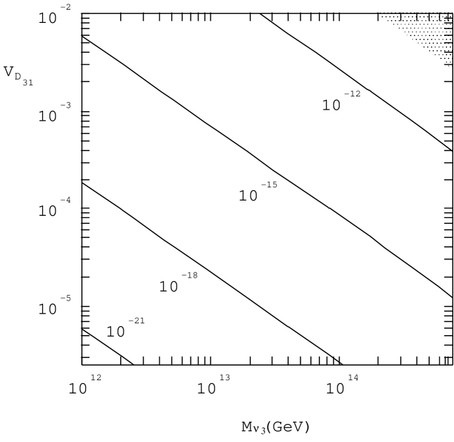
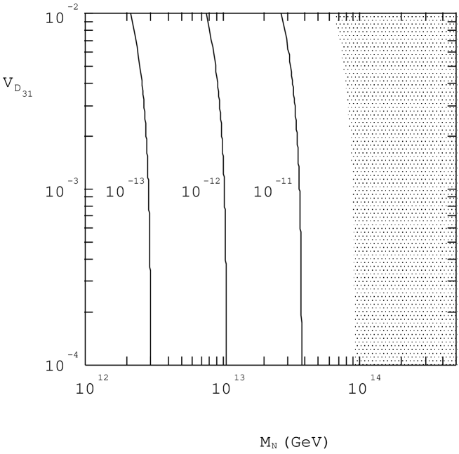
Figure 8: Dependence of the branching ratio of $\mu\to e\gamma$ on the third-generation right-handed neutrino Majorana mass $M_{\nu_{3}}$ and $V_{D31}$ in the MSSM with the right-handed neutrinos. Here the tau neutrino mass is 0.07eV and $V_{D32}=-0.71$, as suggested by the atmospheric neutrino result. We neglect $f_{\nu_{2}}$ here. The curves mean the contours on which the branching ratio of $\mu\to e\gamma$ is $10^{-21},10^{-18},10^{-15}$, and $10^{-12}$, respectively. The shaded region is already excluded experimentally. $\tan\beta$ is set to be 3. The wino mass is 130GeV, the left-handed selectron mass 170GeV, and the Higgsino mass parameter $\mu$ positive.

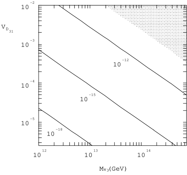
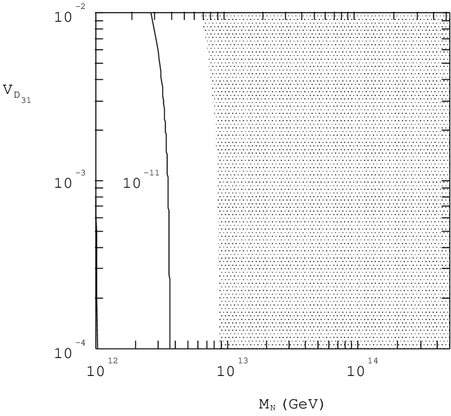
Figure 9: Dependence of the branching ratio of $\mu\to e\gamma$ on the third-generation right-handed neutrino Majorana mass $M_{\nu_{3}}$ and $V_{D31}$ in the MSSM with the right-handed neutrinos. The input parameters are the same as those in Fig. (8) except that we take $\tan\beta=30$ here. The curves mean the contours on which the branching ratio of $\mu\to e\gamma$ is $10^{-18},10^{-15}$, and $10^{-12}$, respectively. The shaded region is already excluded experimentally.

Figure 10: Candidates of the Feynman diagrams which give dominant contributions to $\tau^{+}\to\mu^{+}\gamma$ when $\tan\beta\mathop{}_{\textstyle\sim}^{\textstyle>}1$ and $(m^{2}_{\tilde{e}})_{32}$ is not negligible. The arrows represent the chirality.

Figure 11: Dependence of the branching ratio of $\tau\to\mu\gamma$ on the third-generation right-handed neutrino Majorana mass $M_{\nu_{3}}$ in the SU(5) SUSY GUT with the right-handed neutrinos. Here the tau neutrino mass $m_{\nu_{\tau}}$ is 0.07eV and $V_{D32}=-0.71$, as suggested by the atmospheric neutrino result. We take the bino mass $M_{1}$ 65GeV, the right-handed selectron mass $m_{\tilde{e}_{R}}$ 160GeV. The three curves correspond to the case where $\tan\beta=3,10$, and 30, respectively. The branching ratio becomes larger for larger $\tan\beta$ value.

Figure 12: Candidates of the Feynman diagrams which give dominant contributions to $\mu^{+}\to e^{+}\gamma$ when $\tan\beta\mathop{}_{\textstyle\sim}^{\textstyle>}1$ and the off-diagonal elements of $(m^{2}_{\tilde{e}})$ are non-negligible. The arrows represent the chirality.

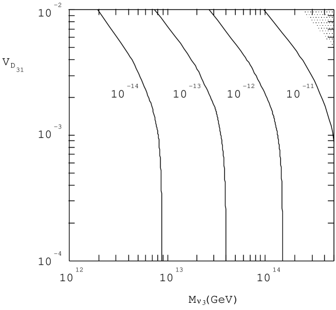
Figure 13: Dependence of the branching ratio of $\mu\to e\gamma$ on the third-generation right-handed neutrino Majorana mass $M_{\nu_{3}}$ and $V_{D31}$ in the SU(5) SUSY GUT with the right-handed neutrinos. Here we take the tau neutrino mass $m_{\nu_{\tau}}$ 0.07eV and the mu neutrino mass is neglected. The curves mean the contours on which the branching ratio of $\mu\to e\gamma$ is $10^{-14},10^{-13},10^{-12}$, and $10^{-11}$, respectively. The shaded region is already excluded experimentally. We take the bino mass $M_{1}$ 65GeV, the right-handed selectron mass $m_{\tilde{e}_{R}}$ 160GeV, and $\tan\beta=3$.

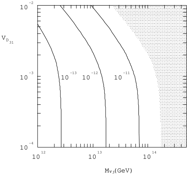
Figure 14: Dependence of the branching ratio of $\mu\to e\gamma$ on the third-generation right-handed neutrino Majorana mass $M_{\nu_{3}}$ and $V_{D31}$ in the SU(5) SUSY GUT with the right-handed neutrinos. The curves mean the contours on which the branching ratio of $\mu\to e\gamma$ is $10^{-13},10^{-12}$, and $10^{-11}$, respectively. The shaded region is already excluded experimentally. The input parameters are the same as those in Fig. (13) except that in this figure $\tan\beta=30$.

Figure 15: Dependence of the branching ratio of $\mu\to e\gamma$ on the typical right-handed neutrino Majorana mass $M_{N}$ and $V_{D31}$ in the SU(5) SUSY GUT with the right-handed neutrinos. We assume the MSW large angle solution, which suggests $m_{\nu_{\mu}}$ to be 0.004eV and $V_{D21}=-0.42$. We take the tau neutrino mass $m_{\nu_{\tau}}$ 0.07eV and $V_{D32}=-0.60$, as suggested by the atmospheric neutrino result. We assume the universality of the right-handed Majorana masses $M_{\nu 1}=M_{\nu 2}=M_{\nu 3}\equiv M_{N}$, for simplicity. The curves mean the contours on which the branching ratio of $\mu\to e\gamma$ is $10^{-13},10^{-12}$, and $10^{-11}$, respectively. The shaded region is already excluded experimentally. We take the bino mass $M_{1}$ 65GeV, the right-handed selectron mass $m_{\tilde{e}_{R}}$ 160GeV. In this figure $\tan\beta=3$.

Figure 16: Dependence of the branching ratio of $\mu\to e\gamma$ on the typical right-handed neutrino Majorana mass $M_{N}$ and $V_{D31}$ in the SU(5) SUSY GUT with the right-handed neutrinos. We assume the MSW large angle solution and the atmospheric neutrino result. All the input parameters are the same as those in Fig. (15) except that we take $\tan\beta=30$ in this figure. The curve means the contour on which the branching ratio of $\mu\to e\gamma$ is $10^{-11}$. The shaded region is already excluded experimentally.

Figure 17: Assignment of the momenta to the external leptons and the external photon in a lepton flavor violating diagram. An anti-charged lepton $e^{+}_{i}$ going into the left vertex with momentum $p$ is annihilated there, and a photon with an outgoing momentum $q$ and an anti-charged lepton $e^{+}_{j}$ with an outgoing momentum $p-q$ are emitted.

Figure 18: Patterns of the chirality flips in the lepton flavor violating diagrams in the $e^{+}_{i}\to e^{+}_{j}\gamma$ decay $(i>j)$ . In the diagrams (a) and (b) the lepton chirality is flipped on the external lines, while in (c) and (d) it is flipped at a vertex of lepton-slepton-neutralino (-chargino). In (e) it flips on the internal slepton line. Chirality flip on the internal slepton line does not occur in the diagram with a virtual chargino because of the absence of the right-handed sneutrino at the low energy region.

References

[1]
J. Ellis and D.V. Nanopoulos, Phys. Lett.110B (1982) 44;
I-Hsiu Lee, Phys. Lett.138B (1984) 121;
Nucl. Phys.B246 (1984) 120.
[2] L. J. Hall, V. A. Kostelecky, and S. Raby,
Nucl. Phys.B267 (1986) 415.
[3]
The Super-Kamiokande Collaboration, Phys. Rev. Lett.81 (1998) 1562;
T. Kajita, hep-ex/9810001.
[4]
K. S. Hirata et al., Phys. Lett.B205 (1988) 416;
Phys. Lett.B280 (1992) 146;
Y. Fukuda et al., Phys. Lett.B335 (1994) 237;
D. Casper et al., Phys. Rev. Lett.66 (1991) 2561;
R. Becker-Szendy et al, Phys. Rev.D46 (1992) 3720.
[6]
T. Yanagida,
in Proceedings of the Workshop on Unified Theory and
Baryon Number of the Universe,
eds. O. Sawada and A. Sugamoto (KEK, 1979) p.95;
M. Gell-Mann, P. Ramond, and R. Slansky,
in Supergravity,
eds. P. van Nieuwenhuizen and D. Freedman
(North Holland, Amsterdam, 1979).
[7] F. Borzumati and A. Masiero, Phys. Rev. Lett.57 (1986) 961.
[8]
J. Hisano, T. Moroi, K. Tobe, M. Yamaguchi, and T. Yanagida,
Phys. Lett.B357 (1995) 579.
[9]
J. Hisano, T. Moroi, K. Tobe, and M. Yamaguchi,
Phys. Rev.D53 (1996) 2442.
[10]
R. Davis, Jr., D. S. Harmer, and K. C. Hoffman,
Phys. Rev. Lett.20 (1968) 1205;
K. S. Hirata et al.,
Phys. Rev. Lett.63 (1989) 16;
Phys. Rev. Lett.65 (1990) 1297.
[11]
S. P. Mikheyev and A. Y. Smirnov,
Yad. Fiz.42 (1985) 1441
[Sov. J. Nucl. Phys.42(1985)913];
Nuovo Cim.C9 (1986) 17;
L. Wolfenstein,
Phys. Rev.D17 (1978) 2369.
[12]
B. Pontecorvo, Zh. Eksp. Teor. Fiz.53 (1967) 1717 ;
S.M. Bilenky and B. Pontecorvo, Phys. Rep.41 (1978) 225;
V. Barger, R.J.N. Phillips and K. Whisnant, Phys. Rev.D24 (1981) 538;
S.L. Glashow and L.M. Krauss, Phys. Lett.B190 (1987) 199.
[13]
J. Bahcall, P.I. Krastev, and A.Yu. Smirnov, hep-ph/9807216.
[14] C. Caso et al. (Particle Data Group),
European Physical JournalC3 (1998) 1.
[15]
N. Arkani-Hamed, H.-C. Cheng, J.L. Feng, and L.J. Hall,
Phys. Rev. Lett.77 (1996) 1937;
Nucl. Phys.B505 (1997) 7.
[16]
J. Hisano, M.M. Nojiri, Y. Shimizu, and M.Tanaka, hep-ph/9808410.
[17] S. M. Bilenky and C. Giunti, hep-ph/9802201.
[18]
Y. Kuno and Y. Okada, Phys. Rev. Lett.77 (1996) 434;
Y. Kuno, A. Maki, and Y. Okada, Phys. Rev.D55 (1997) 2517;
Y. Kuno, KEK-Preprint-97-59.
[19] V. Barger, S. Pakvasa, T. J. Weiler, and K. Whisnant,
hep-ph/9806387.
[20]
J. C. Sen,
Phys. Rev.113 (1959) 679;
K. W. Ford and J. G. Wills,
Nucl. Phys.35 (1962) 295;
R. Pla and J. Bernabeu,
Ann. Fis. (Leipzig)67 (1971) 455;
H. C. Chiang, E. Oset, T. S. Kosmal, A. Faessler, and J. D. Vergados,
Nucl. Phys.A559 (1993) 526.
[21]
J. Bernabeu, E. Nardi and D. Tommasini,
Nucl. Phys.B409 (1993) 63, and references therein.
[22]
MECO collaboration, Proposal to Brookhaven National Laboratory AGS
(Sep, 1997).
[23] R. Barbieri and L. J. Hall, Phys. Lett.B338 (1994) 212.
[24]
R. Barbieri, L. Hall, and A. Strumia,
Nucl. Phys.B445 (1995) 219.
[25]
Phys. Lett.B391 (1997) 341;
Erratum-ibidB397(1997)357.
[26]
N. Arkani-Hamed, H. C. Cheng, and L. J. Hall,
Phys. Rev.D53 (1996) 413.
[27]
J. Hisano, D. Nomura, Y. Okada, Y. Shimizu, and M. Tanaka,
hep-ph/9805367,
to be published in Phys. Rev. D.
[28] J. Hisano, D. Nomura, and T. Yanagida,
Phys. Lett.B437 (1998) 351.
[29]
H. E. Haber and G. L. Kane, Phys. Rep.117 (1985) 75.
Figure 1: The Feynman diagrams which give
dominant contributions to
when and the off-diagonal elements of
the right-handed slepton mass matrix are negligible,
as in the MSSM with the right-handed neutrinos.
In the diagrams, is the element of
the left-handed slepton soft mass matrix.
and
are the left-handed (right-handed) stau and smuon, respectively,
and and
the tau sneutrino and the mu sneutrino.
and are Higgsino,
wino.
The symbol is the Higgsino mass.
The arrows represent the chirality.
Figure 2: Dependence of the branching ratio of
on the left-handed selectron mass in the MSSM
with the right-handed neutrinos.
We take the tau neutrino mass 0.07eV and ,
which are suggested by the atmospheric neutrino result.
is fixed at GeV by imposing a condition
at the gravitational scale.
The dotted line shown in the figure is the present experimental bound.
We set the wino mass 130GeV,
and the Higgsino mass parameter positive.
The mu neutrino mass is neglected.
We take , and 30.
The larger corresponds to the upper curve.
Figure 3: Dependence of the branching ratio of
on the third-generation right-handed neutrino
Majorana mass in the MSSM with the right-handed neutrinos.
The input parameters are the same as those of Fig. (2)
except that in this figure we take GeV and
that we do not impose the condition
but treat as an independent variable.
Here also the larger corresponds to the upper curve.