Abstract

We present a next-to-leading order determination of the gluino-mediated SUSY contributions to $B_{d}$ – $\bar{B}_{d}$ mixing and to the CP asymmetry $a_{J/\psi K_{s}}$ in the framework of the mass-insertion approximation. Using hadronic matrix elements recently computed on the lattice, we obtain improved constraints on the squark-mass splittings.

1 Introduction

With the advent of $B$ factories, $B$ physics is playing a key role in testing the Standard Model (SM) picture of flavour and CP violation and in probing virtual effects from new physics at low energies. In particular, measurements of $\Delta m_{d}$, the mass difference in the $B_{d}$ – $\bar{B}_{d}$ system, and of $a_{J/\psi K_{s}}$, the time-dependent CP asymmetry in $B_{d}\to J/\psi K_{s}$ decays, can be used to put stringent constraints on new-physics contributions to $\Delta B=2$ processes. In terms of the matrix elements of the effective $\Delta B=2$ Hamiltonian we have

$$\Delta m_{d} = 2\,\rm{Abs}[\langle\bar{B}_{d}|{\cal H}_{\rm eff}^{\Delta B=2}|B_{d}\rangle]$$ (1)

$$a_{J/\psi K_{s}} = \sin 2\beta_{\rm eff}\,\sin\Delta m_{d}\,t\,,$$ (2)

where

$$2\beta_{\rm eff}=\,\rm{Arg}[\langle\bar{B}_{d}|{\cal H}_{\rm eff}^{\Delta B=2}|B_{d}\rangle]\,.$$ (3)

Within the SM the value of $\sin 2\beta_{\rm eff}=\sin 2\beta$ can be connected to the CP violation angle $\delta$ of the Unitarity Triangle (UT)

$$\sin 2\beta=\frac{2\sigma\sin\delta(1-\sigma\cos\delta)}{1+\sigma^{2}-2\sigma\cos\delta}\,,$$ (4)

where $\sigma=\sqrt{\rho^{2}+\eta^{2}}$ in the Wolfenstein parametrisation [1]. Assuming that there are no new physics effects in $B_{d}$ – $\bar{B}_{d}$ and $K^{0}$ – $\bar{K}^{0}$ mixing, $\sin 2\beta$ is well determined by the standard UT analysis. For example, ref. [2] quotes

$$\sin 2\beta=0.698\pm 0.066.$$ (5)

The first direct measurements of $a_{J/\psi K_{s}}$ at the $B$ factories suggested a rather low value of the asymmetry [3] which, if confirmed, would have been a hint of new physics [4]–[6]. The most recent world average [7]

$$\sin 2\beta=0.79\pm 0.10\,,$$ (6)

however, is in very good agreement with eq. (5) and therefore does not favour extra contributions. In spite of this, it is worth investigating, in neutral $B$ meson systems, signals of new physics which may emerge in the near future thanks to decreasing experimental errors and theoretical uncertainties. On the one hand, for $\Delta B=2$ transitions, where the SM seems to agree with the data, it is important to improve the theoretical accuracy for constraining new physics contributions to box diagrams. On the other, more accurate predictions of mixing help to uncover signals of new physics in $B$ decay asymmetries, for example $B\to K\pi$ or $B\to K\phi$. These processes are dominated by loop contributions and one measures simultaneously the effect of mixing and CP violation in decay amplitudes, from both SM and new physics virtual particles. Finally, of particular interest is the $B_{s}$–$\bar{B}_{s}$ mixing for which the SM amplitude is real and the phase entirely originates from new physics effects. This may give rise to CP violating effects which would be absent in the SM.

In this work, we aim at testing new-physics effects in $\Delta B=2$ transitions using the most recent experimental and theoretical results: the new data from $B$ factories and the very recent lattice determinations of the relevant matrix elements, which allow the computation of $\Delta m_{d}$ and of $a_{J/\psi K_{s}}$ at the Next-to-Leading Order (NLO), apart from some additional model-dependent ${\cal O}(\alpha_{s}(M_{W}))$ terms. First of all, we present model-independent formulae for $\Delta B=2$ ($B_{d}$ and $B_{s}$) transitions which include all possible new-physics contributions. These formulae are obtained by considering the most general effective Hamiltonian for $\Delta B=2$ processes, ${\cal H}_{\rm eff}^{\Delta B=2}$. We write down the expression for $\Delta m_{d}$ ($\Delta m_{s}$) and for $\beta_{\rm eff}$ in terms of the Wilson coefficients at the electroweak scale, including NLO QCD corrections in the running from $M_{W}$ to $\mu=m_{b}$ [8, 9] and the matrix elements very recently computed in lattice QCD [10], in the same RI-MOM renormalisation scheme. These expressions can be readily used to compute $\Delta m_{d}$ and $\beta_{\rm eff}$ in any extension of the SM.

As a concrete example of physics beyond the SM, we then consider the Minimal Supersymmetric Standard Model (MSSM) with arbitrary soft breaking terms and we study model-independent constraints on the SUSY parameter space coming from $\Delta m_{d}$ and $a_{J/\psi K_{s}}$. We closely follow the analysis of ref. [11], where upper bounds on new sources of flavour and CP violation were obtained from the study of $K^{0}$–$\bar{K}^{0}$ mixing. For earlier analyses, either at tree level or with LO evolution, using naïve Vacuum Insertion Approximation (VIA) $B$ parameters, see refs. [12] and [13] respectively. Ref. [11] and the present work can be considered as first steps toward a full NLO model-independent analysis of flavour and CP violation beyond the SM, with special focus on its most studied extension, namely the general MSSM. We stress that the inclusion of hadronic matrix elements from lattice QCD, for operators renormalised consistently with the Wilson coefficients at the NLO, is highly important to reduce the uncertainties in the study of flavour and CP violation. Indeed, while matrix elements for operators appearing in the SM have been studied for a long time, it was only recently that similar results have been obtained for operators that only come from physics beyond the SM [10, 14]. More work is still to be done along these lines. For example, the large uncertainties in the SUSY constraints from the electric dipole moment of the neutron could be drastically reduced by a lattice computation of the relevant matrix elements [15].

The paper is organised as follows. In the next section we introduce the most general ${\cal H}_{\rm eff}^{\Delta B=2}$ with the inclusion of the NLO QCD corrections in the evolution from the scale of new physics down to low energy. We provide the expression of the Wilson coefficients at the low hadronic scale ($\sim m_{b}$) as a function of the Wilson coefficients and of $\alpha_{s}$ at the “new physics scale”. Section 3 deals with the evaluation of the hadronic matrix elements of the local operators appearing in ${\cal H}_{\rm eff}^{\Delta B=2}$. Here we replace the “traditional” values of the $B$ parameters in the VIA with the values recently obtained from a lattice computation in the RI-MOM scheme [10]. We then turn to SUSY and present in Section 4 the expression of gluino-mediated contributions to ${\cal H}_{\rm eff}^{\Delta B=2}$. As long as we deal with general squark mass matrices, the inclusion of the gluino-mediated FCNC alone is sufficient to get the correct bulk of the SUSY contribution. In specific models corresponding to particularly restricted squark mass matrices, however, there are regions of the SUSY parameter space where charginos, stops and/or charged Higgs are relatively light and their exchange gives contributions even larger than gluinos to FCNC [16]. This happens more easily in the case of $B_{d}$ – $\bar{B}_{d}$ mixing, rather than for $K^{0}$–$\bar{K}^{0}$, because the relevant mixing angles and/or Yukawa couplings are larger in this case. Unfortunately, the experimental information and the theoretical accuracy are presently insufficient to attempt a simultaneous analysis which includes a spanning of the squark mass matrices and of the stop/chargino mass values. For this reason, in this first study which uses the new measurements of $\sin 2\beta$, NLO corrections and lattice $B$ parameters, we include gluino-mediated FCNC only. Our quantitative results are presented in Sect. 5 and summarised in Tables 2 and 3. We perform our computations in the mass insertion approximation [17]. We choose the super-CKM basis for the fermion and sfermion states, where all the couplings of these particles to neutral gauginos are flavour diagonal, while genuine SUSY FC effects are exhibited by the non-diagonal entries of the sfermion mass matrices. Denoting by $\Delta^{2}$ the off-diagonal terms in the sfermion mass matrices (i.e. the mass terms relating sfermions of the same electric charge, but different flavour), the sfermion propagators can be expanded as a series in terms of $\delta=\Delta^{2}/\tilde{m}^{2}$, where $\tilde{m}$ is the average sfermion mass. As long as $\Delta^{2}$ is significantly smaller than $\tilde{m}^{2}$, we can just take the first term of this expansion and then the experimental information concerning FCNC and CP violating phenomena translates into upper bounds on the $\delta$s [11, 12]. Tables 2 and 3 contain new constraints on the parameters $\delta$. With respect to previous analyses, we find that the inclusion of the direct measurements of $\sin 2\beta$ allows imposing quite stringent constraints on $\mathop{\mbox{Im}}\delta_{13}$ [18]. On the theoretical side, as already observed in [11], the QCD evolution from large scales and the use of the lattice $B$ parameters induces sizable changes in the limits on the values of the $\delta$s. The major effect of our improved computation is felt by Left-Right operators.

2 Effective Hamiltonian for $\Delta B=2$ processes beyond the SM

The most general effective Hamiltonian for $\Delta B=2$ processes beyond the SM has the following form:

$${\cal H}_{\rm eff}^{\Delta B=2}=\sum_{i=1}^{5}C_{i}\,Q_{i}+\sum_{i=1}^{3}\tilde{C}_{i}\,\tilde{Q}_{i}$$ (7)

where

$$Q_{1} = \bar{d}^{\alpha}_{L}\gamma_{\mu}b^{\alpha}_{L}\bar{d}^{\beta}_{L}\gamma^{\mu}b^{\beta}_{L}\;,$$

$$Q_{2} = \bar{d}^{\alpha}_{R}b^{\alpha}_{L}\bar{d}^{\beta}_{R}b^{\beta}_{L}\;,$$

$$Q_{3} = \bar{d}^{\alpha}_{R}b^{\beta}_{L}\bar{d}^{\beta}_{R}b^{\alpha}_{L}\;,$$ (8)

$$Q_{4} = \bar{d}^{\alpha}_{R}b^{\alpha}_{L}\bar{d}^{\beta}_{L}b^{\beta}_{R}\;,$$

$$Q_{5} = \bar{d}^{\alpha}_{R}b^{\beta}_{L}\bar{d}^{\beta}_{L}b^{\alpha}_{R}\;,$$

and the operators $\tilde{Q}_{1,2,3}$ are obtained from the $Q_{1,2,3}$ by the exchange $L\leftrightarrow R$. Here $q_{R,L}=P_{R,L}\,q$, with $P_{R,L}=(1\pm\gamma_{5})/2$, and $\alpha$ and $\beta$ are colour indexes. In the case of the $B_{s}$ system one has simply to replace the $d$ with the $s$ quark in the operators appearing in eqs. (2).

The NLO anomalous dimension matrix for the most general ${\cal H}_{\rm eff}^{\Delta F=2}$ has been computed in [8] and the results have been confirmed in [9]. We use the Regularisation-Independent anomalous dimension matrix in the Landau gauge (also known as RI-MOM), since we will make use of matrix elements computed in lattice QCD with the same choice of renormalisation scheme.

A full NLO computation would also require the $O(\alpha_{s})$ corrections to the matching conditions which determine the Wilson coefficients, see eqs. (4) below. These corrections are model-dependent and have been computed only in few specific cases [19, 20]. One might argue that, being of order $\alpha_{s}(M_{S})$ (here and in the following $M_{S}$ represents the scale of new physics), these contributions should be small, as suggested by the cases of the SM and of the two Higgs doublet model [19]. This statement, however, can only be confirmed by explicit computations in specific models. Due to the absence of $O(\alpha_{s})$ corrections to the matching, our ${\cal H}_{\rm eff}^{\Delta F=2}$ are affected by a residual scheme dependence, which would be cancelled by the terms of order $\alpha_{s}(M_{S})$ in the Wilson coefficients $C_{i}(M_{S})$. These terms are model dependent.

Constant	Value	Constant	Value
$m_{B_{d}}$	$5.279$ GeV	$f_{B_{d}}$	$200\pm 30$ MeV
$m^{\overline{MS}}_{d}(2{\rm GeV})$	$7$ MeV	$m^{\overline{MS}}_{b}(m^{\overline{MS}}_{b})$	$4.23$ GeV
$m_{t}$	$174\pm 5$ GeV	$\alpha_{s}(M_{Z})$	$0.119$
$|V_{cb}|$	$(40.7\pm 1.9)\times 10^{-3}$	$|V_{ub}|$	$(3.61\pm 0.46)\times 10^{-3}$

Table 1: Input quantities used in the phenomenological analysis. $m^{\overline{MS}}_{d}$ and $m^{\overline{MS}}_{b}$ are the $\overline{MS}$ masses whereas $m_{t}$ is the pole mass.

The $C_{i}(M_{S})$ are obtained by integrating out all new particles simultaneously at the scale $M_{S}$. We then have to evolve the coefficients down to the hadronic scale $\mu=m_{b}=4.6$ GeV ($m_{b}\equiv m_{b}(\mu=m_{b})$ is the RI-MOM mass), which is the renormalisation scale of the operators used in ref. [10]. By coincidence, $m_{b}$ has the same numerical value as the pole mass, $m_{b}^{pole}=4.6$ GeV, extracted at the NLO from the $\overline{MS}$ mass $m^{\overline{MS}}_{b}(m^{\overline{MS}}_{b})=4.23$ GeV, see Table 1. For consistency, we have to evolve the Wilson coefficients at the same renormalisation scale. The SM contribution can be computed independently and evolved from $M_{W}$ to $\mu$ using the well-known NLO QCD corrections [21].

We give here an analytic formula for the expression of the Wilson coefficients at the scale $\mu=m_{b}$ as a function of the initial conditions at the SUSY scale $C_{i}(M_{S})$ and of $\alpha_{s}(M_{S})$. This formula has been obtained by using, for the SM parameters, the values in Table 1. For $M_{S}>m_{t}$ we obtain

$$C_{r}(m_{b}^{pole})=\sum_{i}\sum_{s}\left(b^{(r,s)}_{i}+\eta\,c^{(r,s)}_{i}\right)\eta^{a_{i}}\,C_{s}(M_{S}),$$ (9)

where, in the evolution of the coefficients from $M_{S}$, we have chosen $M_{S}=(M_{\tilde{g}}+M_{\tilde{q}})/2$ and $\eta=\alpha_{s}(M_{S})/\alpha_{s}(m_{t})$. The magic numbers are given below:

$$\begin{array}[]{l l}a_{i}=(0.286,-0.692,0.787,-1.143,0.143)&\\ &\\ b^{(11)}_{i}=(0.865,0,0,0,0),&c^{(11)}_{i}=(-0.017,0,0,0,0),\\ b^{(22)}_{i}=(0,1.879,0.012,0,0),&c^{(22)}_{i}=(0,-0.18,-0.003,0,0),\\ b^{(23)}_{i}=(0,-0.493,0.18,0,0),&c^{(23)}_{i}=(0,-0.014,0.008,0,0),\\ b^{(32)}_{i}=(0,-0.044,0.035,0,0),&c^{(32)}_{i}=(0,0.005,-0.012,0,0),\\ b^{(33)}_{i}=(0,0.011,0.54,0,0),&c^{(33)}_{i}=(0,0.000,0.028,0,0),\\ b^{(44)}_{i}=(0,0,0,2.87,0),&c^{(44)}_{i}=(0,0,0,-0.48,0.005),\\ b^{(45)}_{i}=(0,0,0,0.961,-0.22),&c^{(45)}_{i}=(0,0,0,-0.25,-0.006),\\ b^{(54)}_{i}=(0,0,0,0.09,0),&c^{(54)}_{i}=(0,0,0,-0.013,-0.016),\\ b^{(55)}_{i}=(0,0,0,0.029,0.863),&c^{(55)}_{i}=(0,0,0,-0.007,0.019),\\ \end{array}$$ (10)

and we have only written the non-vanishing entries. The magic numbers for the evolution of $\tilde{C}_{1-3}$ are the same as the ones for the evolution of $C_{1-3}$. Formulae (9) and (10) are combined with the $B$ parameters evaluated at $m_{b}^{pole}=4.6$ GeV in the MOM-RI scheme [10], given in eqs. (13) below . In this way it is possible to compute the contribution to $\Delta m_{d,s}$ and $\beta_{\rm eff}$ at the NLO in QCD for any model of new physics in which the new contributions with respect to the SM originate from extra heavy particles. One just has to plug in the expression for the $C_{i}$ evaluated at the large energy scale $M_{S}$ in his favourite model. When the $O(\alpha_{s})$ corrections to the $C_{i}(M_{S})$ are available, one can obtain a full NLO, regularisation-independent result; in the cases where this corrections have not been computed yet, the results contain a residual systematic uncertainty of order $\alpha_{s}(M_{S})$. We note that, due to the presence of large entries in the NLO anomalous dimension matrix, a systematic uncertainty is present in the QCD evolution from the SUSY scale to the hadronic one. This uncertainty stems from different ways of writing the NLO evolution matrix, which differ by terms of ${\cal O}(\alpha^{2}_{s})$, and has been taken into account in the numerical analysis as uncertainty in the numerical value of the magic numbers. For this reason we have presented only the significant figures of the magic numbers, which have an uncertainty of one unit on the last digit. The only exception is $c^{(44)}_{4}$ for which the uncertainty is 3 units.

3 Hadronic Matrix Elements

The matrix elements of the operators $Q_{i}$ between neutral $B$ mesons in the VIA are given by:

$$\langle\bar{B}_{d}|Q_{1}|B_{d}\rangle_{\rm VIA} = \frac{1}{3}m_{B_{d}}f_{B_{d}}^{2}\;,$$

$$\langle\bar{B}_{d}|Q_{2}|B_{d}\rangle_{\rm VIA} = -\frac{5}{24}\left(\frac{m_{B_{d}}}{m_{b}+m_{d}}\right)^{2}m_{B_{d}}f_{B_{d}}^{2}\;,$$

$$\langle\bar{B}_{d}|Q_{3}|B_{d}\rangle_{\rm VIA} = \frac{1}{24}\left(\frac{m_{B_{d}}}{m_{b}{}+m_{d}}\right)^{2}m_{B_{d}}f_{B_{d}}^{2}\;,$$ (11)

$$\langle\bar{B}_{d}|Q_{4}|B_{d}\rangle_{\rm VIA} = \left[\frac{1}{24}+\frac{1}{4}\left(\frac{m_{B_{d}}}{m_{b}+m_{d}}\right)^{2}\right]m_{B_{d}}f_{B_{d}}^{2}\;,$$

$$\langle\bar{B}_{d}|Q_{5}|B_{d}\rangle_{\rm VIA} = \left[\frac{1}{8}+\frac{1}{12}\left(\frac{m_{B_{d}}}{m_{b}+m_{d}}\right)^{2}\right]m_{B_{d}}f_{B_{d}}^{2}\;,$$

where $m_{B_{d}}$ is the mass of the $B_{d}$ meson and $m_{b}$ and $m_{d}$ are the masses of the $b$ and $d$ quarks respectively. Note that the normalisation of the operators used in this paper differs by a factor of $2m_{B_{d}}$ from the one used in ref. [10]. Here and in the following, the same expressions of the $B$ parameters of the operators $Q_{1-3}$ are valid for the operators $\tilde{Q}_{1-3}$, since strong interactions preserve parity. In the case of the $B_{s}$ system one has simply to replace the $d$ with the $s$ quark in the operators and expressions appearing in eqs. (3).

In the case of the renormalised operators, we define the $B$ parameters as follows:

$$\langle\bar{B}_{d}|\hat{Q}_{1}(\mu)|B_{d}\rangle = \frac{1}{3}m_{B_{d}}f_{B_{d}}^{2}B_{1}(\mu)\;,$$

$$\langle\bar{B}_{d}|\hat{Q}_{2}(\mu)|B_{d}\rangle = -\frac{5}{24}\left(\frac{m_{B_{d}}}{m_{b}(\mu)+m_{d}(\mu)}\right)^{2}m_{B_{d}}f_{B_{d}}^{2}B_{2}(\mu)$$

$$\langle\bar{B}_{d}|\hat{Q}_{3}(\mu)|B_{d}\rangle = \frac{1}{24}\left(\frac{m_{B_{d}}}{m_{b}(\mu)+m_{d}(\mu)}\right)^{2}m_{B_{d}}f_{B_{d}}^{2}B_{3}(\mu)$$ (12)

$$\langle\bar{B}_{d}|\hat{Q}_{4}(\mu)|B_{d}\rangle = \frac{1}{4}\left(\frac{m_{B_{d}}}{m_{b}(\mu)+m_{d}(\mu)}\right)^{2}m_{B_{d}}f_{B_{d}}^{2}B_{4}(\mu)$$

$$\langle\bar{B}_{d}|\hat{Q}_{5}(\mu)|B_{d}\rangle = \frac{1}{12}\left(\frac{m_{B_{d}}}{m_{b}(\mu)+m_{d}(\mu)}\right)^{2}m_{B_{d}}f_{B_{d}}^{2}B_{5}(\mu)\ ,$$

where the notation $\hat{Q}_{i}(\mu)$ (or simply $\hat{Q}_{i}$) denotes the operators renormalised at the scale $\mu$. For consistency with the calculation of the $B$ parameters in ref. [10], the quark masses, evolved at the scale $\mu$, must be computed in the Landau RI-MOM scheme [23, 24]. With the numbers in Table 1, this corresponds to $m_{b}=m_{b}(m_{b})=4.6$ GeV and $m_{d}(m_{b})=5.4$ MeV (RI-MOM) .

A few words of explanation are necessary at this point. The $B$ parameter of the matrix element $\langle\bar{B}_{d}|Q_{1}|B_{d}\rangle$ has been extensively studied on the lattice due to its phenomenological relevance [25, 26], and used in many UT analyses [2, 27]. For the other operators, instead, all the studies beyond the SM have used the VIA $B$ parameters, which in some cases, as will be shown below, is a crude approximation. The numerical results for the $B$ parameters $B_{i}(\mu)$ refer to the RI-MOM scheme. We have used the same definition of the $B$ parameters as in ref. [10] from which we have taken the values. In our numerical study, we have used

$$B_{1}(m_{b})=0.87(4)^{+5}_{-4}$$   ,   ,

  ,   ,

  .

(13)

We added a conservative $\pm 10$% systematic error to the errors quoted above, based on previous experience on discretisation, extrapolation and quenching effects. In the cases where a comparison has been possible, the quenching effects for all the $B$ parameters computed so far have always been found much smaller than all other uncertainties.

4 Effective Hamiltonian for $\Delta B=2$ processes in SUSY

In this Section, we describe the computation of gluino-mediated contributions to ${\cal H}_{\rm eff}^{\Delta B=2}$ at the NLO in QCD.

Several cases may be considered: i) $m_{\tilde{q}}\sim m_{\tilde{g}}$, ii) $m_{\tilde{q}}\ll m_{\tilde{g}}$ and iii) $m_{\tilde{q}}\gg m_{\tilde{g}}$ , where $m_{\tilde{q}}$ is the average squark mass and $m_{\tilde{g}}$ is the gluino mass. Case ii), in which $m_{\tilde{q}}\ll m_{\tilde{g}}$, cannot be realised in the framework considered here, in which the soft SUSY breaking terms are introduced at the Planck scale. This is due to the fact that the evolution from the Planck to the electroweak scale forbids such a mass hierarchy. In fact, neglecting the effects of Yukawa couplings and A-terms, one obtains in the down sector the following approximate expression for the ratio $x=m^{2}_{\tilde{g}}/m_{\tilde{q}}^{2}$ at the electroweak scale, in terms of the value $x_{0}$ at the Planck scale [28]:

$$x\simeq\frac{9x_{0}}{1+7x_{0}}\longrightarrow\frac{9}{7}\,.$$ (14)

Even if one starts at the super-large scale with an extreme hierarchy between squark and gluino masses ($x_{0}\gg 1$), at the electroweak scale the two masses will be of the same order. For this reason, we will not consider the case $m_{\tilde{q}}\ll m_{\tilde{g}}$ in our analysis. Case iii), in which $m_{\tilde{q}}\gg m_{\tilde{g}}$, can be realised in some special models, such as effective supersymmetry [30] or models with a light gluino [31]. The NLO corrections in this case have been computed in ref. [32]. In this first study, however, we do not consider these cases and present only results for the case $m_{\tilde{q}}\sim m_{\tilde{g}}$.

The mass insertion approximation, which we have adopted in our analysis, presents the major advantage that one does not need the full diagonalisation of the sfermion mass matrices to perform a test of FCNC in the SUSY model under consideration. It is enough to compute ratios of the off-diagonal over the diagonal entries of the sfermion mass matrices and compare the results with the general bounds on the $\delta$s which we provide here from $\Delta m_{B_{d}}$ and $a_{J/\psi K_{s}}$. This formulation of the mass insertion approximation in terms of the parameters $\delta$ is particularly suitable for model-independent analyses, but involves two further assumptions: the smallness of the off-diagonal mass terms with respect to the diagonal ones, and the degeneracy of the diagonal mass terms in the super-CKM basis. The latter assumption, related to the use of the average squark mass $\tilde{m}$, is well justified in our case, since, on quite general grounds, one does not expect a sizable non-degeneracy of the down-type squarks. In SUSY GUT it may happen that the sbottom mass is smaller than the $d$ and $s$ squark masses. Also in this case, namely for non-degenerate diagonal mass terms, however, it is possible to define a generalised mass insertion approximation [29] and apply the methods exposed in this paper.

There exist four different $\delta$ mass-insertions connecting flavours $d$ and $b$ along a sfermion propagator: $\left(\delta^{d}_{13}\right)_{LL}$, $\left(\delta^{d}_{13}\right)_{RR}$, $\left(\delta^{d}_{13}\right)_{LR}$ and $\left(\delta^{d}_{13}\right)_{RL}$. The indexes $L$ and $R$ refer to the helicity of the fermion partners. The amplitude for $\Delta B=2$ transitions in the full theory at the LO is given by the computation of the diagrams in fig. 1.

Figure 1: Feynman diagrams for $\Delta B=2$ transitions, with $h,k,l,m=\{L,R\}$.

At the lowest order in QCD, in the basis of eq. (2), the Wilson coefficients are given by [12]:

$$C_{1} = -\frac{\alpha_{s}^{2}}{216m_{\tilde{q}}^{2}}\left(24\,x\,f_{6}(x)+66\,\tilde{f}_{6}(x)\right)\left(\delta^{d}_{13}\right)^{2}_{LL}\,,$$

$$C_{2} = -\frac{\alpha_{s}^{2}}{216m_{\tilde{q}}^{2}}\,204\,x\,f_{6}(x)\left(\delta^{d}_{13}\right)^{2}_{RL}\,,$$

$$C_{3} = \frac{\alpha_{s}^{2}}{216m_{\tilde{q}}^{2}}\,36\,x\,f_{6}(x)\left(\delta^{d}_{13}\right)^{2}_{RL}\,,$$

$$C_{4} = -\frac{\alpha_{s}^{2}}{216m_{\tilde{q}}^{2}}\biggl{[}\left(504\,x\,f_{6}(x)-72\,\tilde{f}_{6}(x)\right)\left(\delta^{d}_{13}\right)_{LL}\left(\delta^{d}_{13}\right)_{RR}$$

$$-132\,\tilde{f}_{6}(x)\left(\delta^{d}_{13}\right)_{LR}\left(\delta^{d}_{13}\right)_{RL}\biggr{]}\,,$$

$$C_{5} = -\frac{\alpha_{s}^{2}}{216m_{\tilde{q}}^{2}}\biggl{[}\left(24\,x\,f_{6}(x)+120\,\tilde{f}_{6}(x)\right)\left(\delta^{d}_{13}\right)_{LL}\left(\delta^{d}_{13}\right)_{RR}$$

$$-180\,\tilde{f}_{6}(x)\left(\delta^{d}_{13}\right)_{LR}\left(\delta^{d}_{13}\right)_{RL}\biggr{]}\,,$$

$$\tilde{C}_{1} = -\frac{\alpha_{s}^{2}}{216m_{\tilde{q}}^{2}}\left(24\,x\,f_{6}(x)+66\,\tilde{f}_{6}(x)\right)\left(\delta^{d}_{13}\right)^{2}_{RR}\,,$$

$$\tilde{C}_{2} = -\frac{\alpha_{s}^{2}}{216m_{\tilde{q}}^{2}}\,204\,x\,f_{6}(x)\left(\delta^{d}_{13}\right)^{2}_{LR}\,,$$

$$\tilde{C}_{3} = \frac{\alpha_{s}^{2}}{216m_{\tilde{q}}^{2}}\,36\,x\,f_{6}(x)\left(\delta^{d}_{13}\right)^{2}_{LR}\,,$$ (15)

where $x=m^{2}_{\tilde{g}}/m_{\tilde{q}}^{2}$ and the functions $f_{6}(x)$ and $\tilde{f}_{6}(x)$ are given by:

$$f_{6}(x) = \frac{6(1+3x)\ln x+x^{3}-9x^{2}-9x+17}{6(x-1)^{5}}\;,$$

$$\tilde{f}_{6}(x) = \frac{6x(1+x)\ln x-x^{3}-9x^{2}+9x+1}{3(x-1)^{5}}\;.$$ (16)

In the absence of $O(\alpha_{s})$ corrections to the matching, we interpret the $C_{i}$ given above as coefficients computed at the large energy scale $M_{S}\sim m_{\tilde{q}}\sim m_{\tilde{g}}$, i.e. $C_{i}\equiv C_{i}(M_{S})$.

Figure 2: Allowed regions in the ($\gamma$, $\mathop{\mbox{Re}}(\delta^{d}_{13})_{LL}$, $\mathop{\mbox{Im}}(\delta^{d}_{13})_{LL}$) space with $(\delta^{d}_{13})_{LL}$ only (left) and $(\delta^{d}_{13})_{LL}=(\delta^{d}_{13})_{RR}$ (right). The two lower plots are the corresponding projections in the $\mathop{\mbox{Re}}(\delta^{d}_{13})_{LL}$–$\mathop{\mbox{Im}}(\delta^{d}_{13})_{LL}$ plane. Different colours denote values of $\gamma$ belonging to different quadrants.

Figure 3: Allowed regions in the ($\gamma$, $\mathop{\mbox{Re}}(\delta^{d}_{13})_{LR}$, $\mathop{\mbox{Im}}(\delta^{d}_{13})_{LR}$) space with $(\delta^{d}_{13})_{LR}$ only (left) and $(\delta^{d}_{13})_{LR}=(\delta^{d}_{13})_{RL}$ (right). The two lower plots are the corresponding projections in the $\mathop{\mbox{Re}}(\delta^{d}_{13})_{LR}$–$\mathop{\mbox{Im}}(\delta^{d}_{13})_{LR}$ plane. Different colours denote values of $\gamma$ belonging to different quadrants.

5 Numerical Analysis of $\Delta B=2$ Processes

In this section, we illustrate the procedure followed in our analysis and give the main results. $\Delta m_{d}$ and $\sin 2\beta$ are defined in terms of the matrix element $\langle\bar{B}_{d}|{\cal H}_{\rm eff}^{\Delta B=2}|B_{d}\rangle$ which we schematically write as

$$\langle\bar{B}_{d}|{\cal H}_{\rm eff}^{\Delta B=2}|B_{d}\rangle = \mathop{\mbox{Re}}{\cal A}_{SM}+i\,\mathop{\mbox{Im}}{\cal A}_{SM}+$$ (17)

$${\cal A}_{SUSY}\mathop{\mbox{Re}}(\delta^{d}_{13})_{AB}^{2}+i\,{\cal A}_{SUSY}\mathop{\mbox{Im}}(\delta^{d}_{13})_{AB}^{2}\,,$$

where ${\cal A}_{SM}$ is the Standard Model contribution which depends on the CKM matrix parameters, in particular on the CP violation phase $\gamma$. $(\delta^{d}_{13})_{AB}$ denotes the generic effective coupling appearing in eq. (4). In the following, for simplicity, the constraints are obtained by imposing that the sum of the SUSY contributions proportional to a single $(\delta^{d}_{13})_{AB}$ parameter and the SM contribution does not exceed by more than $1\sigma$ the experimental value of $\Delta m_{d}$ and $\sin 2\beta$. This is justified (a posteriori) by noting that the constraints on different $(\delta^{d}_{13})_{AB}$ parameters exhibit a hierarchical structure, and therefore interference effects between different contributions would require a large amount of fine tuning. We consider the following four cases: i) $(\delta^{d}_{13})_{LL}$ only; ii) $(\delta^{d}_{13})_{LL}=(\delta^{d}_{13})_{RR}$; iii) $(\delta^{d}_{13})_{LR}$ only; iv) $(\delta^{d}_{13})_{LR}=(\delta^{d}_{13})_{RL}$. For this reason, in all the cases considered here, the amplitude in eq. (17) only depends on a single $(\delta^{d}_{13})_{AB}^{2}$.

	$|\mathop{\mbox{Re}}(\delta^{d}_{13})_{LL}|$			$|\mathop{\mbox{Re}}(\delta^{d}_{13})_{LL=RR}|$
$x$	TREE	LO	NLO	TREE	LO	NLO
0.25	$4.9\times 10^{-2}$	$5.4\times 10^{-2}$	$6.2\times 10^{-2}$	$3.1\times 10^{-2}$	$2.0\times 10^{-2}$	$1.9\times 10^{-2}$
1.0	$1.1\times 10^{-1}$	$1.2\times 10^{-1}$	$1.4\times 10^{-1}$	$3.4\times 10^{-2}$	$2.2\times 10^{-2}$	$2.1\times 10^{-2}$
4.0	$6.0\times 10^{-1}$	$6.7\times 10^{-1}$	$7.0\times 10^{-1}$	$4.7\times 10^{-2}$	$3.0\times 10^{-2}$	$2.8\times 10^{-2}$
	$|\mathop{\mbox{Im}}(\delta^{d}_{13})_{LL}|$			$|\mathop{\mbox{Im}}(\delta^{d}_{13})_{LL=RR}|$
$x$	TREE	LO	NLO	TREE	LO	NLO
0.25	$1.1\times 10^{-1}$	$1.2\times 10^{-1}$	$1.3\times 10^{-1}$	$1.3\times 10^{-2}$	$8.0\times 10^{-3}$	$8.0\times 10^{-3}$
1.0	$2.6\times 10^{-1}$	$2.8\times 10^{-1}$	$3.0\times 10^{-1}$	$1.5\times 10^{-2}$	$9.0\times 10^{-3}$	$9.0\times 10^{-3}$
4.0	$2.6\times 10^{-1}$	$2.9\times 10^{-1}$	$3.4\times 10^{-1}$	$2.0\times 10^{-2}$	$1.3\times 10^{-2}$	$1.2\times 10^{-2}$
	$|\mathop{\mbox{Re}}(\delta^{d}_{13})_{LR}|$			$|\mathop{\mbox{Re}}(\delta^{d}_{13})_{LR=RL}|$
$x$	TREE	LO	NLO	TREE	LO	NLO
0.25	$3.4\times 10^{-2}$	$2.7\times 10^{-2}$	$3.0\times 10^{-2}$	$3.8\times 10^{-2}$	$2.7\times 10^{-2}$	$2.6\times 10^{-2}$
1.0	$3.9\times 10^{-2}$	$3.0\times 10^{-2}$	$3.3\times 10^{-2}$	$8.3\times 10^{-2}$	$5.4\times 10^{-2}$	$5.2\times 10^{-2}$
4.0	$5.3\times 10^{-2}$	$4.1\times 10^{-2}$	$4.5\times 10^{-2}$	$1.2\times 10^{-1}$	$2.5\times 10^{-1}$	$-$
	$|\mathop{\mbox{Im}}(\delta^{d}_{13})_{LR}|$			$|\mathop{\mbox{Im}}(\delta^{d}_{13})_{LR=RL}|$
$x$	TREE	LO	NLO	TREE	LO	NLO
0.25	$7.6\times 10^{-2}$	$6.0\times 10^{-2}$	$6.6\times 10^{-2}$	$1.5\times 10^{-2}$	$9.0\times 10^{-3}$	$9.0\times 10^{-3}$
1.0	$8.7\times 10^{-2}$	$6.6\times 10^{-2}$	$7.4\times 10^{-2}$	$3.6\times 10^{-2}$	$2.4\times 10^{-2}$	$2.3\times 10^{-2}$
4.0	$1.2\times 10^{-1}$	$9.2\times 10^{-2}$	$1.0\times 10^{-1}$	$2.7\times 10^{-1}$	$5.7\times 10^{-1}$	$-$

Table 2: Maximum allowed values for $|\mathop{\mbox{Re}}\left(\delta^{d}_{ij}\right)_{AB}|$ and $|\mathop{\mbox{Im}}\left(\delta^{d}_{ij}\right)_{AB}|$, with $A,B=(L,R)$, for an average squark mass $m_{\tilde{q}}=500$ GeV and for different values of $x=m_{\tilde{g}}^{2}/m_{\tilde{q}}^{2}$. We give the results in the following cases: i) with the tree level Wilson coefficients, namely without evolution from $M_{S}$ to $m_{b}$, and VIA $B$ parameters, denoted by TREE; ii) with LO evolution and VIA $B$ parameters, denoted by LO; iii) with NLO evolution and lattice $B$ parameters, denoted by NLO. The missing entries correspond to cases in which no constraint was found for $|\left(\delta^{d}_{ij}\right)_{AB}|<0.9$.

	$|\mathop{\mbox{Re}}(\delta^{d}_{13})_{LL}|$		$|\mathop{\mbox{Re}}(\delta^{d}_{13})_{LL=RR}|$
$x$	$m_{\tilde{q}}=250$ GeV	$m_{\tilde{q}}=1000$ GeV	$m_{\tilde{q}}=250$ GeV	$m_{\tilde{q}}=1000$ GeV
0.25	$-$	$1.3\times 10^{-1}$	$-$	$3.8\times 10^{-2}$
1.0	$6.5\times 10^{-2}$	$3.1\times 10^{-1}$	$1.0\times 10^{-2}$	$4.2\times 10^{-2}$
4.0	$3.2\times 10^{-1}$	$-$	$1.4\times 10^{-2}$	$5.9\times 10^{-2}$
	$|\mathop{\mbox{Im}}(\delta^{d}_{13})_{LL}|$		$|\mathop{\mbox{Im}}(\delta^{d}_{13})_{LL=RR}|$
$x$	$m_{\tilde{q}}=250$ GeV	$m_{\tilde{q}}=1000$ GeV	$m_{\tilde{q}}=250$ GeV	$m_{\tilde{q}}=1000$ GeV
0.25	$-$	$2.8\times 10^{-1}$	$-$	$1.6\times 10^{-2}$
1.0	$1.3\times 10^{-1}$	$5.0\times 10^{-1}$	$4.0\times 10^{-3}$	$1.8\times 10^{-2}$
4.0	$1.5\times 10^{-1}$	$-$	$6.0\times 10^{-3}$	$2.5\times 10^{-2}$
	$|\mathop{\mbox{Re}}(\delta^{d}_{13})_{LR}|$		$|\mathop{\mbox{Re}}(\delta^{d}_{13})_{LR=RL}|$
$x$	$m_{\tilde{q}}=250$ GeV	$m_{\tilde{q}}=1000$ GeV	$m_{\tilde{q}}=250$ GeV	$m_{\tilde{q}}=1000$ GeV
0.25	$-$	$6.2\times 10^{-2}$	$-$	$5.3\times 10^{-2}$
1.0	$1.5\times 10^{-2}$	$6.8\times 10^{-2}$	$2.5\times 10^{-2}$	$1.1\times 10^{-1}$
4.0	$2.2\times 10^{-2}$	$9.4\times 10^{-2}$	$-$	$-$
	$|\mathop{\mbox{Im}}(\delta^{d}_{13})_{LR}|$		$|\mathop{\mbox{Im}}(\delta^{d}_{13})_{LR=RL}|$
$x$	$m_{\tilde{q}}=250$ GeV	$m_{\tilde{q}}=1000$ GeV	$m_{\tilde{q}}=250$ GeV	$m_{\tilde{q}}=1000$ GeV
0.25	$-$	$1.4\times 10^{-1}$	$-$	$2.1\times 10^{-2}$
1.0	$3.3\times 10^{-2}$	$1.5\times 10^{-1}$	$9.0\times 10^{-3}$	$4.5\times 10^{-2}$
4.0	$4.8\times 10^{-2}$	$2.2\times 10^{-1}$	$-$	$-$

Table 3: Maximum allowed values for $|\mathop{\mbox{Re}}\left(\delta^{d}_{ij}\right)_{AB}|$ and $|\mathop{\mbox{Im}}\left(\delta^{d}_{ij}\right)_{AB}|$, with $A,B=(L,R)$, for an average squark mass $m_{\tilde{q}}=250$ GeV or $1000$ GeV and for different values of $x=m_{\tilde{g}}^{2}/m_{\tilde{q}}^{2}$. We give the results with NLO evolution and lattice $B$ parameters. The missing entries correspond to cases in which no constraint was found for $|\left(\delta^{d}_{ij}\right)_{AB}|<0.9$.

The procedure used in our numerical analysis is the following:

• We scan over all possible values of $\gamma$ between $0$ and $2\pi$ since, in the presence of SUSY effects, this parameter is no longer constrained by the UT analysis. Indeed, $\epsilon_{K}$ may be subject to large SUSY contributions due to the $(\delta^{d}_{12})_{AB}$ couplings and the value of $\gamma$ can be very different from the SM value;

• for a fixed value of $\gamma$, we scan over $\mathop{\mbox{Re}}(\delta^{d}_{13})_{AB}$ and $\mathop{\mbox{Im}}(\delta^{d}_{13})_{AB}$ between $-1$ and $1$;

• we let the other experimental and theoretical parameters, in particular the $B$ parameters, vary within the ranges given in Table 1 and in Eq. (13);

• in the ($\gamma$, $\mathop{\mbox{Re}}(\delta^{d}_{13})_{AB}$, $\mathop{\mbox{Im}}(\delta^{d}_{13})_{AB}$) space, we select the region where the predicted values of $\Delta m_{d}$ and $\sin 2\beta$ lie within $1\sigma$ from the measured values.

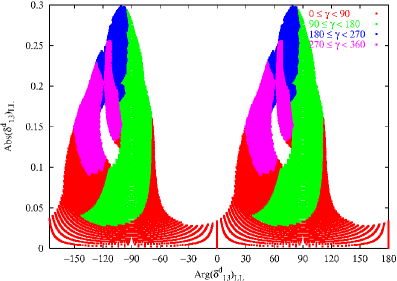
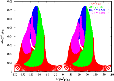
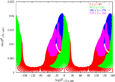
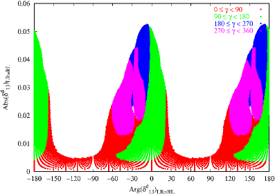
As can be seen from Eq. (17), the amplitude only depends on the square of the coupling, $(\delta^{d}_{13})_{AB}^{2}$. Therefore, the selected values of $(\delta^{d}_{13})_{AB}$ have a twofold ambiguity ($\mathop{\mbox{Re}}(\delta^{d}_{13})_{AB}\to-\mathop{\mbox{Re}}(\delta^{d}_{13})_{AB}$ and $\mathop{\mbox{Im}}(\delta^{d}_{13})_{AB}\to-\mathop{\mbox{Im}}(\delta^{d}_{13})_{AB}$) as will be evident from our results.

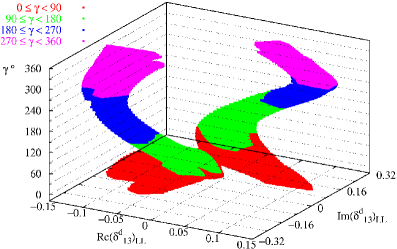
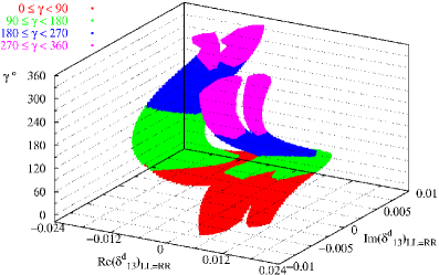
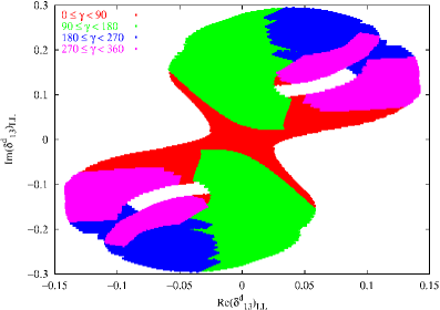
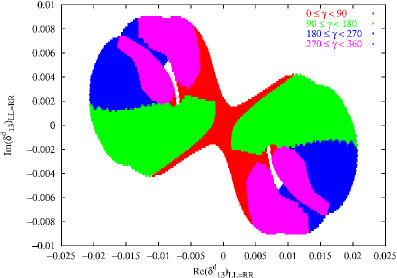
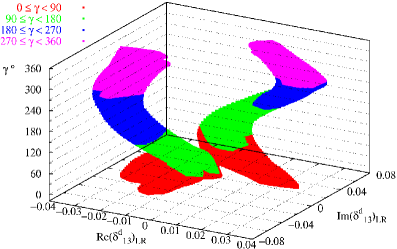
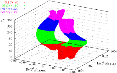
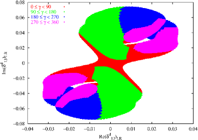
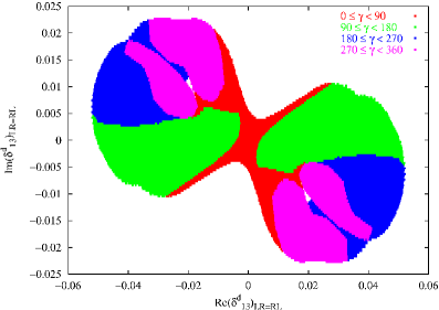
We are ready to discuss the physics results. In Figs. 2–3, for $m_{\tilde{q}}=m_{\tilde{g}}=500$ GeV, we show the allowed regions in the ($\gamma$, $\mathop{\mbox{Re}}(\delta^{d}_{13})_{AB}$, $\mathop{\mbox{Im}}(\delta^{d}_{13})_{AB}$) space and the corresponding projections on the ($\mathop{\mbox{Re}}(\delta^{d}_{13})_{AB}$, $\mathop{\mbox{Im}}(\delta^{d}_{13})_{AB}$) plane. For the readers’ convenience, we have coloured regions corresponding to $\gamma$ in the four quadrants with different colours. An alternative way of presenting our results is given in Fig. 4 where the allowed values of Abs$(\delta^{d}_{13})_{AB}$ are plotted as a function of Arg$(\delta^{d}_{13})_{AB}$ .

We give the maximum allowed values of $|\mathop{\mbox{Re}}(\delta^{d}_{13})_{AB}|$ and $|\mathop{\mbox{Im}}(\delta^{d}_{13})_{AB}|$ in Table 2 for $x=0.25$, $1$ and $4$. We also give results for $m_{\tilde{q}}=250$ GeV and $1000$ GeV in Table 3. We find that the constraints on the $(\delta^{d}_{13})_{AB}$ parameters are less effective by a factor from 10 to 100 with respect to those extracted on $(\delta^{d}_{12})_{AB}$ from $\Delta S=2$ transitions. The reason for this difference is twofold. On the one hand, one naturally expects constraints of the order of $\sin^{3}\theta_{c}$ for $B_{d}$ – $\bar{B}_{d}$ mixing and $\sin^{5}\theta_{c}$ for $K^{0}$–$\bar{K}^{0}$ mixing, dictated by the top contribution in the SM amplitude. On the other, in the $K^{0}$–$\bar{K}^{0}$ case, LR contributions are chirally enhanced, so that limits coming from chirality-changing operators are more effective. Obviously, specific models of flavour, where $(\delta^{d}_{12})_{AB}$ and $(\delta^{d}_{13})_{AB}$ are correlated, can constrain the squark-mass splittings more severely. In these cases one could even attempt the inclusion of chargino contributions to the mixing [18, 33]. Our general formulae for the effective Hamiltonian and the magic numbers remain valid, and the phenomenological analysis can be carried out along the same lines.

We now discuss the difference between our results and those obtained with tree level or LO Wilson coefficients and VIA matrix elements. In this case, with our definition of the $B$ parameters given in eq. (3), with $\kappa=(m_{b}/m_{B_{d}})^{2}=0.76$, we have used

$$B_{1}^{VIA}=1.0$$  ,   ,

  ,   ,

  .

(18)

With NLO corrections and lattice $B$ parameters, the constraints are generically looser than using LO and VIA $B$ parameters. The theoretical uncertainties of the NLO constraints are, however, much smaller. In the LL=RR case, the NLO bounds are even more stringent than the LO ones, in spite of the uncertainties on the $B$ parameters. The most striking effect is obtained in the LR=RL case for $x=4$. Here, the strong cancellation taking place at the LO is exacerbated by NLO corrections, jeopardising any possibility to constrain $(\delta^{d}_{13})_{LR}$ in this case. Clearly, given the cancellation, this result should be interpreted with care and verified by calculations in any given model.

With the future measurements of $\Delta m_{s}$ at proton colliders, and hopefully of the corresponding CP violating effects in $B_{s}$ mixing and decays, it will be soon possible to perform a similar analysis for the $B_{s}$ system. Work along this line is in progress [34].

Figure 4: Allowed values of Abs$(\delta^{d}_{13})_{LR}$ as a function of Arg$(\delta^{d}_{13})_{AB}$ in the four considered cases. Different colours denote values of $\gamma$ belonging to different quadrants.

6 Conclusions

In this work we have provided an improved determination of the gluino-mediated SUSY contributions to $B_{d}$ – $\bar{B}_{d}$ mixing and to the CP asymmetry $a_{J/\psi K_{s}}$ in the framework of the mass-insertion method. The improvement consists in introducing the NLO QCD corrections to ${\cal H}_{\rm eff}^{\Delta B=2}$ [8, 9] and in replacing the VIA matrix elements with their recent lattice computation [10]. As a glimpse at Table 2 readily reveals, these improvements affect previous results in a different way, according to the operators of ${\cal H}_{\rm eff}^{\Delta B=2}$ that one considers. The effect is particularly large for Left-Right operators.

We have provided an analytic formula for the most general low-energy ${\cal H}_{\rm eff}^{\Delta B=2}$ at the NLO, in terms of the Wilson coefficients at the high energy scale. This formula can be readily used to compute $\Delta m_{d}$ and $\sin 2\beta$ in any extension of the SM with new heavy particles.

FCNC and CP violating phenomena (in particular in $B$ physics) are promising candidates for some indirect SUSY signal before LHC, and are in many ways complementary to direct SUSY searches. From this point of view the theoretical effort to improve as much as possible our precision on FCNC computations in a SUSY model-independent framework is certainly worth and, hopefully, rewarding.

References

• [1] L. Wolfenstein, Phys. Rev. Lett.  51 (1983) 1945.
• [2] M. Ciuchini et al., JHEP 0107 (2001) 013 [arXiv:hep-ph/0012308].
• [3] T. Affolder et al. [CDF Collaboration], Phys. Rev. D 61 (2000) 072005 [arXiv:hep-ex/9909003]; D. G. Hitlin [BABAR Collaboration], arXiv:hep-ex/0011024; H. Aihara [BELLE Collaboration], arXiv:hep-ex/0010008.
• [4] A. J. Buras and R. Buras, Phys. Lett. B 501 (2001) 223 [arXiv:hep-ph/0008273].
• [5] G. Eyal, Y. Nir and G. Perez, JHEP 0008 (2000) 028 [arXiv:hep-ph/0008009].
• [6] A. Masiero, M. Piai and O. Vives, Phys. Rev. D 64 (2001) 055008 [arXiv:hep-ph/0012096].
• [7] This average has been taken from http://parodi.home.cern.ch/parodi/ckm/ckm.html and it is based on the following references: Opal Collaboration, Eur. Phys. J. C5 (1998) 379; Aleph Collaboration, Phys. Lett. B492 (2000) 259; CDF Collaboration, Phys. Rev. Lett. 81 (1998) 5513; Babar Collaboration, Phys. Rev. Lett. 86 (2001) 2515; Belle Collaboration, Phys. Rev. Lett. 87 (2001) 091802.
• [8] M. Ciuchini, E. Franco, V. Lubicz, G. Martinelli, I. Scimemi and L. Silvestrini, Nucl. Phys. B 523 (1998) 501 [arXiv:hep-ph/9711402].
• [9] A. J. Buras, M. Misiak and J. Urban, Nucl. Phys. B 586 (2000) 397 [arXiv:hep-ph/0005183].
• [10] D. Becirevic, V. Gimenez, G. Martinelli, M. Papinutto and J. Reyes, arXiv:hep-lat/011091; see also arXiv:hep-lat/0110117.
• [11] M. Ciuchini et al., JHEP 9810, 008 (1998) [arXiv:hep-ph/9808328].
• [12] F. Gabbiani and A. Masiero, Nucl. Phys. B 322 (1989) 235 ; J. S. Hagelin, S. Kelley and T. Tanaka, Nucl. Phys. B 415 (1994) 293 ; E. Gabrielli, A. Masiero and L. Silvestrini, Phys. Lett. B 374 (1996) 80 [arXiv:hep-ph/9509379]; F. Gabbiani, E. Gabrielli, A. Masiero and L. Silvestrini, Nucl. Phys. B 477 (1996) 321 [arXiv:hep-ph/9604387];
• [13] J. A. Bagger, K. T. Matchev and R. J. Zhang, Phys. Lett. B 412 (1997) 77 [arXiv:hep-ph/9707225].
• [14] L. Conti et al., Nucl. Phys. Proc. Suppl.  73 (1999) 315 [arXiv:hep-lat/9809162]; A. Donini, V. Gimenez, L. Giusti and G. Martinelli, Phys. Lett. B 470 (1999) 233 [arXiv:hep-lat/9910017].
• [15] G. Martinelli, plenary talk at LATTICE 2001, The XIX International Symposium on Lattice Field Theory, August 19 - 24, 2001, Berlin, hep-lat/0112011.
• [16] M. Misiak, S. Pokorski and J. Rosiek, Adv. Ser. Direct. High Energy Phys.  15 (1998) 795 [arXiv:hep-ph/9703442].
• [17] L. J. Hall, V. A. Kostelecky and S. Raby, Nucl. Phys. B 267 (1986) 415.
• [18] C. K. Chua and W. S. Hou, arXiv:hep-ph/0110106.
• [19] J. Urban, F. Krauss, U. Jentschura and G. Soff, Nucl. Phys. B 523 (1998) 40 [arXiv:hep-ph/9710245].
• [20] T-F. Feng et al., Phys. Rev. D 63 (2001) 015013 [arXiv:hep-ph/0008029].
• [21] A. J. Buras, M. Jamin and P. H. Weisz, Nucl. Phys. B 347 (1990) 491.
• [22] A. J. Buras, S. Jager and J. Urban, Nucl. Phys. B 605 (2001) 600 [arXiv:hep-ph/0102316].
• [23] G. Martinelli, C. Pittori, C.T. Sachrajda, M. Testa and A. Vladikas, Nucl. Phys. B 445 (1995) 81.
• [24] A. Donini, V. Gimenez, G. Martinelli, M. Talevi and A. Vladikas, Eur. Phys. J. C 10 (1999) 121 [arXiv:hep-lat/9902030].
• [25] C. W. Bernard, Nucl. Phys. Proc. Suppl.  94 (2001) 159 [arXiv:hep-lat/0011064].
• [26] S. Ryan, plenary talk at LATTICE 2001, The XIX International Symposium on Lattice Field Theory, August 19 - 24, 2001, Berlin, arXiv:hep-lat/0111010.
• [27] A. Hocker, H. Lacker, S. Laplace and F. Le Diberder, Eur. Phys. J. C 21 (2001) 225 [arXiv:hep-ph/0104062].
• [28] D. Choudhury, F. Eberlein, A. Konig, J. Louis and S. Pokorski, Phys. Lett. B 342 (1995) 180 [arXiv:hep-ph/9408275].
• [29] A. J. Buras, A. Romanino and L. Silvestrini, Nucl. Phys. B 520 (1998) 3 [arXiv:hep-ph/9712398].
• [30] A. G. Cohen, D. B. Kaplan and A. E. Nelson, Phys. Lett. B 388 (1996) 588 [arXiv:hep-ph/9607394].
• [31] G. R. Farrar, Phys. Rev. Lett.  53 (1984) 1029.
• [32] R. Contino and I. Scimemi, Eur. Phys. J. C 10 (1999) 347, [arXiv:hep-ph/9809437].
• [33] A. Masiero, M. Piai, A. Romanino and L. Silvestrini, Phys. Rev. D 64 (2001) 075005 [arXiv:hep-ph/0104101].
• [34] D. BeΔ‡ireviΔ‡, et al., in preparation.