Two-loop neutrino masses with large R-parity violating interactions in supersymmetry

Abstract

We attempt to reconcile large trilinear R-parity violating interactions in a supersymmetric (SUSY) theory with the observed pattern of neutrino masses and mixing. We show that, with a restricted number of such interaction terms with the $\lambda^{\prime}$-type couplings in the range (0.1-1.0), it is possible to forbid one-loop contributions to the neutrino mass matrix. This is illustrated with the help of a ‘working example’ where an econnomic choice of SUSY parameters is made, with three non-vanishing and ‘large’ R-parity violating terms in the superpotential. The two-loop contributions in such a case can not only generate the masses in the requisite order but can also lead us to specific allowed regions of the parameter space.

I Introduction

Neutrinos are massless to all orders in perturbation theory in the standard model (SM). However, the ever-accumulating data on solar, atmospheric and reactor neutrinos challenge us with the inescapable fact that neutrinos are massive and their physical states are mixtures of the flavour eigenstates sno ; bando ; rean . The SM has to be extended for explaining this. The simplest extension is the inclusion of ‘sterile’ right-handed neutrinos, whereby neutrinos may either acquire just Dirac masses or, with lepton number violation, participate in the see-saw mechanism which accounts for their ultra-light character.

An alternative mechanism is provided by the supersymmetric (SUSY) extension of the SM with renormalizable $R$-parity ($R_{p}$) violating terms in the Lagrangian SUSY1 ; godb . The fact that baryon and lepton numbers are but accidentally conserved in the SM entails the possibility of $R_{p}=(-1)^{3B+L+2S}$ being violated in SUSY, where $B$, $L$ and $S$ are baryon number, lepton number and spin respectively. In order to avoid unacceptably fast proton decay, either $B$ or $L$ must be conserved, while the other may be violated. In the latter situation, small Majorana mass terms for neutrinos (with $\Delta L=2$) are generated, without the requirement of any additional fields godb . Thus, the neutrino sector may be looked upon as a motivation for such $L$-violating interactions.

The multiplicative conservation of $R$-parity prevents the lightest SUSY particle (LSP) from decaying, as $R_{p}$ equals $+1$ for all SM particles and $-1$ for the superparticles. All possibilities of $R_{p}$-violation are encapsulated in the following terms of the superpotential:

$$W_{\not R}=\lambda_{ijk}L_{i}L_{j}E^{c}_{K}+\lambda^{\prime}_{ijk}L_{i}Q_{j}D^{c}_{K}+\lambda^{\prime\prime}_{ijk}U^{c}_{i}D^{c}_{j}D^{c}_{K}+\epsilon_{i}L_{i}H_{2},$$ (1)

where the first two trilinear terms and the bilinear term are $\Delta L=1$ and the third term is $\Delta B=1$. Since we are interested in neutrino masses, let us assume that $B$ is conserved, and that $R_{p}$ is broken through $L$-violating couplings only. Moreover, we are neglecting the bilinear terms $\epsilon_{i}L_{i}H_{2}$ (on which we will comment later), and consider the trilinear $\lambda^{\prime}_{ijk}$-type couplings only to illustrate our point. Elaborate studies in the recent years have led to constraints at various levels on these couplings dreiner-1 ; gautam . The pertinent gauge-invariant terms trilinear in particle/sparticle fields are given by

$$\lambda^{\prime}_{ijk}\left[{\tilde{\nu}}^{i}_{L}\bar{d}^{k}_{R}d^{j}_{L}+{\tilde{d}}^{j}_{L}\bar{d}^{k}_{R}\nu^{i}_{L}+({\tilde{d}}^{k}_{R})^{*}(\bar{\nu}^{i}_{L})^{c}d^{j}_{L}-{\tilde{e}}^{i}_{L}\bar{d}^{k}_{R}u^{j}_{L}-{\tilde{u}}^{j}_{L}\bar{d}^{k}_{R}e^{i}_{L}-({\tilde{d}}^{k}_{R})^{*}(\bar{e}^{i}_{L})^{c}u^{j}_{L}\right]+{\rm h.c.}.$$ (2)

It is easy to see from above that the $\lambda^{\prime}_{ijk}$-type couplings (27 of them altogether) can generate neutrino masses at the loop level, where the largest contribution comes from $\lambda^{\prime}_{i33}$. We expect that all of the entries in the neutrino mass matrix should lie well within 1 eV. A generic expression for one-loop masses generated in this fashion is oneloop

$$(m^{1-\rm loop}_{\nu})_{ij}\simeq\frac{3}{8\pi^{2}}m^{d}_{k}m^{d}_{p}M_{SUSY}\frac{1}{{m}^{2}_{{\tilde{q}}}}\lambda^{\prime}_{ikp}\lambda^{\prime}_{jpk},$$ (3)

where $m^{d}_{k}$ is the down-type quark mass of $k^{\rm th}$ generation, ${m}^{2}_{{\tilde{q}}}$ is the (average) squark mass squared, and $M_{SUSY}~{}(\sim\mu$, the Higgsino mass parameter) is the effective scale of SUSY breaking. If the masses thus induced have to answer to the observed pattern, then a SUSY breaking mass scale of about 500 GeV would in general imply $\lambda^{\prime}\sim 10^{-5}-10^{-4}$ oneloop . A similar conclusion follows for $\lambda$-type terms, too.

The question to ask is: are all trilinear R-parity violating couplings thus destined to be so small, irrespective of all other phenomenological considerations? For example, will the observation of any process which requires large values of some $\lambda^{\prime}$-terms mean that we need some additional mechanism to explain the neutrino mass pattern? We wish to demonstrate in this paper that it is not so, so long as one can eliminate the one-loop contributions but allow two-loop ones, through a limited number of $\lambda^{\prime}_{ijk}$-terms. This drastically reduces the number of the $\lambda^{\prime}$ terms whose signals may be of interest at the Large Hadron Collider (LHC), be it for direct observation or through indirect radiative effects.

Situations where $R_{p}$-violating two-loop effects can contribute substantially compared to those at the one-loop level have been studied in earlier works borz1 . In contrast, let us assume here a scenario in which there is a ‘minimal’ set of non-zero large ($\sim 0.1-1.0$) $\lambda^{\prime}$- type couplings at the weak scale. One can clearly see from Eq. (3) that for such large $\lambda^{\prime}$’s, it is impossible to explain the existing neutrino data, without going into unrealistically high values for $m^{2}_{{\tilde{q}}}$, if both $\lambda^{\prime}_{ikp}$ and $\lambda^{\prime}_{jpk}$ are allowed for the relevant $\{ij\}$-sets. A way out of this problem would be to postulate this minimal set of large $\lambda^{\prime}$’s, of such composition that the above combinations do not exist, and the relevant interaction terms of Eq. (2) contribute to the neutrino mass matrix at the two-loop level (and beyond) only. At this level, together with the usual loop suppression factors with respect to the one-loop contributions, there will be additional suppression coming from the parameters describing left-right mixing among different flavours in the squark mass matrices fcnc . It is thus interesting to see whether these two suppression factors together may offset the ‘largeness’ of $\lambda^{\prime}$’s, ultimately yielding contributions to neutrino mass matrix in accordance with the existing neutrino data.

While there are no direct evidences of the Nature favouring any particular $R_{p}$-violating coupling over the others, one may, as a starting point, take those that are supported by the low-energy data. As a case in point, it has recently been advocated in soumitra:bsds that a minimal set of three $R_{p}$-violating couplings can simultaneously explain two interesting observations in flavour physics. The first one, as shown by the UTfit Collaboration, is the existence of a sizable deviation of the $B_{s}$-$\overline{B}_{s}$ mixing phase, $\beta_{s}$, from its SM expectation, which is close to zero. The second one is the abnormally large leptonic branching ratio of the $D_{s}$ meson dobrescu-kronfeld . In ref. soumitra:bsds , it was found that one must have large $\lambda^{\prime}_{223}$ ($\lambda^{\prime}_{323}$) to explain the recent data on $D_{s}\to\mu\nu$ ($D_{s}\to\tau\nu$) dsdata , and in addition either $\lambda^{\prime}_{212}$ or $\lambda^{\prime}_{312}$ on similar order, contributing to the phase in $B_{s}$ mixing. The $D_{s}$ anomaly stems from a very accurate determination of the decay constant, $f_{D_{s}}$, on the lattice by the HPQCD Collaboration hpqcd . It has been pointed out in lubicz:0807.4605 that further clarifications are needed on some of the approximations used in hpqcd , and prior to that, it may be advisable to use a more conservative estimate of $f_{D_{s}}$, namely, ($250\pm 15$) MeV. Such a value is not in direct conflict with the experimental number ($273\pm 10$) MeV, and if one wishes to invoke $R_{p}$-violation to explain the slight excess, one may use smaller values of the relevant couplings than those used in soumitra:bsds . On the whole, we take the above result as a motivating feature of our analysis, without committing ourselves too decidedly on any specific numerical values.

It may be in order to spell out at this stage how general our approach is, by re-iterating its main motivation. We would like to emphasize that we are not just attempting to compute two-loop diagrams contributing to neutrino masses, which have not been evaluated before. Nor is the sole purpose of this investigation to account for the claims on $D_{s}$ decays. The principal point made by us is that one can reconcile large R-parity violating couplings and neutrino masses, if only a subset of all possible couplings of such nature exist. If there is indication of large couplings, the subset must further be determined by the impossibility of generating one-loop neutrino masses. Two-loop contributions are tenable in such situations, and they can fit the entire neutrino mass matrix answering to the experimental constraints. An essential additional ingredient of this mechanism is SUSY flavour violation through squark mass matrices. We have stressed on identifying the minimum possible number of $R_{p}$-and flavour-violating parameters. This in a way restricts the set of contributing diagrams, but this feature is characteristic of a minimal choice and not of the specific couplings chosen, especially if the sfermions of different flavours are of comparable mass, a feature well-motivated from the suppression of flavour-changing processes. Thus this study reflects an entire set of possibilities rather than the property of some specific R-parity violating couplings. Let us also mention that the values of all $R_{p}$-violating couplings are taken to be those at the electroweak scale and in the mass eigenbasis of the quarks.

The paper is arranged as follows. In section II we discuss the overall requirements in generating neutrino masses at the two-loop level only, using $R_{p}$ violating couplings of the $\lambda^{\prime}$-type. Some features of the two-loop contributions are outlined in section III, while in section IV we test the validity of the scheme on a numerical basis. Section V is on some correlated signals of the relevant couplings that may be tested at the LHC. We summarize and conclude in section VI. Some representative expressions related to the loop integrals are included in the Appendix.

II The parameters relevant for two-loop effects

Let us try to identify a minimal set of parameters that are required to generate a neutrino mass matrix at no less than the two-loop level. Of course, one requires a set of non-zero $\lambda^{\prime}$ which can be allowed to lie in the range $0.1-1$. As will be explained below, one further requires the parameters controlling flavour violation in the squark sector in order to generate the mass matrix in a way consistent with observations.

Next, we recall the pattern of the three-family neutrino mass matrix in the flavour basis, assuming, without any loss of generality, that the charged lepton mass matrix is diagonal in this basis. The constraints on the mixing angles are pdg

$$\sin^{2}(2\theta_{12})=0.86^{+0.03}_{-0.04}\ \Rightarrow\ \theta_{12}=(33.89\pm 1.44)^{\circ}\,,\ \ \ \sin^{2}(2\theta_{23})>0.92\ \Rightarrow\ \theta_{23}>36.8^{\circ}\,,$$ (4)

and $\sin^{2}(2\theta_{12})<0.19$. We assume the bilarge mixing scheme so that $\theta_{23}=\pi/4$ and $\theta_{13}=0$ massmatrix ,

$$M_{\nu}=\ \left(\!\begin{array}[]{ccc}m_{1}c^{2}+m_{2}s^{2}&\frac{cs}{\sqrt{2}}(-m_{1}+m_{2})&\frac{cs}{\sqrt{2}}(m_{1}-m_{2})\\ \frac{cs}{\sqrt{2}}(-m_{1}+m_{2})&\frac{1}{2}(m_{1}s^{2}+m_{2}c^{2}+m_{3})&\frac{1}{2}(-m_{1}s^{2}-m_{2}c^{2}+m_{3})\\ \frac{cs}{\sqrt{2}}(m_{1}-m_{2})&\frac{1}{2}(-m_{1}s^{2}-m_{2}c^{2}+m_{3})&\frac{1}{2}(m_{1}s^{2}+m_{2}c^{2}+m_{3})\end{array}\!\right)\,,$$ (8)

where $m_{1}$, $m_{2}$, $m_{3}$ are the mass eigenvalues, and $s=\sin\theta_{12}$, $c=\cos\theta_{12}$, $\theta_{ij}$ being the mixing angle between the $i$th and the $j$th family. From this matrix one can easily take up the specific scenarios of normal ($m_{3}>>m_{2}\gtrsim m_{1}$) or inverted ($m_{2}\gtrsim m_{1}>>m_{3}$) hierarchy or that of degenerate neutrinos ($m_{1}\simeq m_{2}\simeq m_{3}$). One can take $m_{1}=0$ for normal hierarchy (NH) and $m_{3}=0$ for inverted hierarchy (IH), without any loss of generality. In the case of NH, the existing data require (at 95% confidence limit)

$$m^{2}_{2}=(7.60\pm 0.35)\times 10^{-5}~{}{\rm eV}^{2},~{}\left|m^{2}_{3}-m^{2}_{2}\right|=(2.50\pm 0.27)\times 10^{-3}~{}{\rm eV}^{2},$$ (9)

and $s^{2}=0.3$. The corresponding numbers for IH and degenerate neutrinos (DN) are

$$m^{2}_{2}-m^{2}_{1}=(7.60\pm 0.35)\times 10^{-5} \!\!\!\!{\rm eV}^{2},~{}\left|m^{2}_{2}-m^{2}_{3}\right|\simeq\left|m^{2}_{1}-m^{2}_{3}\right|=(2.50\pm 0.27)\times 10^{-3}~{}{\rm eV}^{2},$$

and

$$m_{1}\simeq m_{2}\simeq m_{3}\simeq O(10^{-1})~{}{\rm eV}$$ (11)

respectively bando2 .

Let us first try to understand intuitively the properties of the ‘minimal set’.

• There must be no less than three $\lambda^{\prime}$ type couplings, each with a different leptonic index, for the three neutrinos.

• To prevent mass generation at one-loop, couplings like $\lambda^{\prime}_{ijj}$, which generate diagonal entries of the neutrino mass matrix, are forbidden.

• Similarly, combinations like $\lambda^{\prime}_{ikl}\lambda^{\prime}_{jlk}$ are forbidden to prevent the off-diagonal entries at the one-loop level.

• In fact, $\lambda^{\prime}_{ikl}\lambda^{\prime}_{jmk}$ combinations are also not allowed, since they can generate one-loop masses with the mass insertion $\delta_{ml}^{LR}$.

This leaves us with a limited number of possible choices.

As already discussed in Section I, our choice of the supersymmetric scenario is partially motivated by the explanation of the results on $D_{s}$ decays . We thus include $\lambda^{\prime}_{223}$ and $\lambda^{\prime}_{323}$ in our minimal set of $\lambda^{\prime}$-type couplings, and propose that their values be allowed to be large, consistent with the individual constraints. It is easy to see from the relevant interaction terms (the second and third terms of Eq. (2)) that we need one more $\lambda^{\prime}_{ijk}$ with $i=1$, in order to have contributions to the elements in the first row and the first column of $M_{\nu}$. The choices that we thus have are $\lambda^{\prime}_{112}$, $\lambda^{\prime}_{121}$, $\lambda^{\prime}_{113}$, $\lambda^{\prime}_{131}$ and $\lambda^{\prime}_{123}$.

Figure 1: A typical one-loop diagram contributing to neutrino masses. It should be remembered that corresponding to each such diagram there is one with $\nu_{i}$ and $\nu^{c}_{j}$ flipped.

Let us clarify the last criterion mentioned above. As a first choice, let us choose $\lambda^{\prime}_{112}$. It is then easy to see from Figure 1 that there are non-vanishing one-loop contributions to the $(1,2)$ and $(1,3)$ elements of the neutrino mass matrix. This is because of the fact that the quark and squark mass matrices of the same charge are not in general diagonal simultaneously; the evolution of the squark mass parameters from the high scale of SUSY breaking always tend to destroy such alignment. The resulting possibility of a flavour transition as well as a chirality flip along the down-type squark propagator allows one to obtain some one-loop contributions to the neutrino mass matrix. These contributions are driven by a parameter $\delta^{LR}_{13}$ of mass-squared dimension, which is basically the corresponding off-diagonal term in the down-type squark mass matrix . Such diagrams are not suppressed enough to balance the large values ($O(0.1)$) of $\lambda^{\prime}_{223}$ and $\lambda^{\prime}_{323}$ and give admissibly small entries for the $(1,2)$ and $(1,3)$ elements of the neutrino mass matrix. So, a non-zero $\lambda^{\prime}_{112}$ will not normally serve our purpose. Besides, the phenomenological constraint on $\lambda^{\prime}_{112}$ makes it an inappropriate candidate for the demonstration of the effects of large $R_{p}$ violating interactions. Following similar arguments, the choice of $\lambda^{\prime}_{131}$ should be abandoned in our minimal set of $\lambda^{\prime}$’s.

On the contrary, none among $\lambda^{\prime}_{121}$, $\lambda^{\prime}_{113}$ and $\lambda^{\prime}_{123}$ can give one-loop contributions to the neutrino mass matrix. So in principle any one of them can be included in the minimal set together with $\lambda^{\prime}_{223}$ and $\lambda^{\prime}_{323}$, to generate neutrino mass at two-loop level. Note that the choice of $\lambda^{\prime}_{123}$ puts a single squark mixing parameter at our disposal, namely, the one describing the second-and third-family squark mixing ($\delta_{23}^{LR}$). Thus we would have a set of four independent parameters: $\lambda^{\prime}_{223}$, $\lambda^{\prime}_{323}$, $\lambda^{\prime}_{123}$ and $\delta_{23}^{LR}$. However, as will be evident from our numerical results in Section IV, it is difficult to fit the six independent elements of $M_{\nu}$ with experimental data with just these four parameters.

Choosing $\lambda^{\prime}_{113}$, on the other hand, will involve $\delta_{13}^{LR}$, the first- and third-family squark mixing parameter, for generating the elements of $M_{\nu}$ in the first row and first column, and $\delta_{23}$ for the rest of the matrix elements (from now on, we will drop the chirality superscript on the $\delta$s, since the only type that we will ever be interested in are those of the $LR$ type in the down-squark sector). This means that for this choice we have a set of five independent parameters comprising of ($\lambda^{\prime}_{223}$, $\lambda^{\prime}_{323}$, $\lambda^{\prime}_{113}$, $\delta_{23}$ and $\delta_{13}$). In Section IV we will see that in this case we are able to fit elements of $M_{\nu}$ with the existing constraints. In a similar way, the choice of $\lambda^{\prime}_{121}$ also leads to the same number of independent parameters. However, for the latter choice, some two-loop contributions would be suppressed further by the ratio $m_{s}/m_{b}$, making the two-loop effects undesirably small, as we shall see in Section IV.

Thus, our selected parameter space consists of a minimal set of three $O(0.1)$ $\lambda^{\prime}$’s, namely $\lambda^{\prime}_{223}$, $\lambda^{\prime}_{323}$ and $\lambda^{\prime}_{113}$, and two non-zero squark mixing parameters $\delta_{13}$ and $\delta_{23}$, generating neutrino masses at the two-loop level. All other parameters are set to be zero at the weak scale. Also, we will work under the assumption of all the $\lambda^{\prime}$’s being real.

In our calculation, we scale the squark mixing parameter $\delta_{ij}$ by the factor $m_{b}M_{SUSY}$, and define a dimensionless parameter ${\Delta_{ij}}=\delta_{ij}/(m_{b}M_{SUSY})$, with the already specified connotation $\Delta_{ij}=\Delta^{LR}_{ij}$. The various loop contributions which involve flavour violation and require a chirality flip in the (down-type) squark propagator are expressed in terms of $\Delta_{13}$ and $\Delta_{23}$.

The coupling $\lambda^{\prime}_{113}$ is bounded from charged current universality barger-giudice-han as well as processes like $\pi^{+}\to e^{+}\nu_{e}$. Here we use a 99% confidence level bound of $|\lambda^{\prime}_{113}|\leq 0.15$. As we shall see, this relative smallness of $\lambda^{\prime}_{113}$ leads to a distinct preference of the NH scenario of neutrino masses over IH or DN.

$\lambda^{\prime}_{223}$ and $\lambda^{\prime}_{323}$, the other two couplings, can be large, even $O(1)$. We have checked that the recent CLEO constraint on lepton flavour violation in $\Upsilon\to\mu\tau$ cleo:lfv is consistent with this upper limit.

Ref. 2 of dreiner-1 quotes a weak scale bounds of $|{\lambda^{\prime}}_{113}|,|{\lambda^{\prime}}_{i23}|\leq 0.39$. These limits arise from the need to prevent tachyonic sneutrinos even at the Grand Unified Theory (GUT) scale decarlos . The maximum value at the GUT scale is driven by the input parameters; for the set known as SPS1a, this comes out to be about 0.13. When run down at the $M_{Z}$ scale, the coupling increases threefold and the bound becomes $0.39$. One can easily relax this bound for other choices of the GUT scale input parameters.

The dimensionless parameters $\Delta_{ij}$ can be constrained from various flavour-changing neutral current (FCNC) processes. For those that we are interested in, $\Delta_{13}$ is constrained from $B^{0}$-$\overline{B}{}^{0}$ mixing to be less than 5.2, and $\Delta_{23}$ is constrained from the inclusive $b\to s\gamma$ branching ratio to be less than 1.0.

Let us mention again that this is just one of several possible choices. Following the rules laid down earlier, one must have three $\lambda^{\prime}$ type couplings and two $\delta$-type squark mixing parameters. However, some of the possible choices are extremely constrained from data. For example, the choice of $\lambda^{\prime}_{121}$, $\lambda^{\prime}_{221}$, $\lambda^{\prime}_{323}$, $\delta_{21}^{LR}$ and $\delta_{23}^{LR}$ is severely restricted by the absence of leptonic flavour-violating decays $\pi^{0}\to e\mu$, $\phi\to e\mu$, $B\to e(\mu)\tau$ etc.

III The two-loop contributions

Having shown that there are no one-loop contributions to the neutrino mass matrix $M_{\nu}$, let us enlist and compute the two-loop contributions that are driven by the three nonzero $\lambda^{\prime}$ type couplings and two $\delta$ parameters. We work in the ’t Hooft-Feynman gauge.

Figure 2: Two-loop diagrams that make leading contributions to neutrino masses. The contributions in the three different diagrams are proportional to (a) $\lambda^{\prime}_{ipk}\lambda^{\prime}_{jk^{\prime}p^{\prime}}\Delta^{LR}_{pp^{\prime}}V_{u_{n}d_{k}}V^{\ast}_{u_{n}d_{k^{\prime}}}$ (b) $\lambda^{\prime}_{ipk}\lambda^{\prime}_{jk^{\prime}p^{\prime}}\Delta^{LR}_{pp^{\prime}}V_{u_{k^{\prime}}d_{k}}$ (c) $\lambda^{\prime}_{ipk}\lambda^{\prime}_{jk^{\prime}p^{\prime}}\Delta^{LR}_{kp^{\prime}}V_{u_{p}d_{k^{\prime}}}$. For our choice of $\lambda^{\prime}$’s in (c), $k=p^{\prime}=3$ and thus $\Delta_{kp^{\prime}}=1$, so that there is no squark flavour violation. The flipped diagrams, too, will contribute as usual.

Although the individual diagrams are divergent, the very fact that there is no counterterm at the tree-level for the interactions generated at higher loop levels immediately tells us that the end result is finite. This is ensured when all diagrams including all possible fields and their superpartners are taken into account.

Figure 2 represents three classes of diagrams that turn out to be dominant in our study. A full list of generic expressions for the loop-factors arising from these diagrams is provided in the Appendix. The amplitude corresponding to diagram 2(a) for the $(1,1)$ and $(i,j)$ elements of $M_{\nu}$, where $i,j=2,3$, is found to be

$$\left[M^{\rm 2a}_{\nu}\right]_{11} \sim \frac{m_{d}m_{b}}{(m^{2}_{d}-m^{2}_{b})}{\Delta}_{13}\xi_{t},$$

$$\left[M^{\rm 2a}_{\nu}\right]_{ij} \sim \frac{m_{s}m_{b}}{(m^{2}_{s}-m^{2}_{b})}{\Delta}_{23}\xi^{\prime}_{t}$$ (12)

respectively, where $\xi_{t}=V^{*}_{ts}V_{tb}$, and $\xi^{\prime}_{t}=V^{*}_{td}V_{tb}$. The loop functions have been left out of these expressions. For the $(1,2)$ and $(1,3)$ elements of $M_{\nu}$, the contribution from diagram 2(a) contains two separate parts proportional to the two factors written above, along with the appropriate loop functions multiplying each of them.

The amplitude for diagram 2(b) vanishes when mediated by $W^{\pm}$ (but not the charged Higgs or Goldstone field), which follows from the details of $\gamma$-matrix algebra. For the diagonal entries of the neutrino mass matrix, this diagram yields

$$\left[M^{\rm 2b}_{\nu}\right]_{11} \sim V_{ub}\frac{m_{b}m_{d}}{M^{2}_{W}}{\Delta}_{13}x_{e}x_{u},$$

$$\left[M^{\rm 2b}_{\nu}\right]_{22} \sim V_{cb}\frac{m_{b}m_{s}}{M^{2}_{W}}{\Delta}_{23}x_{\mu}x_{c},$$

$$\left[M^{\rm 2b}_{\nu}\right]_{33} \sim V_{cb}\frac{m_{b}m_{s}}{M^{2}_{W}}{\Delta}_{23}x_{\tau}x_{c}$$ (13)

where $x_{a}=m^{2}_{a}/M^{2}_{W}$ for $a=e,\mu,\tau,u,c$. Each of the off-diagonal matrix elements (1,2), (1,3) and (2,3) is a sum of two terms which are respectively proportional to the first and second, first and third and second and third factors written above, again with the corresponding loop functions. In general, being proportional to the squares of lepton masses, the contribution of diagram 2(b) are suppressed compared to those of Figure 2(a). Diagram 2(c) is particularly interesting, since there is no flavour change required along the internal squark-line in this diagram. Thus, these diagrams do not have the suppression by $\Delta$-factors. Nevertheless, this diagram has an overall lepton mass dependence. So ultimately it contributes more than diagram 2(b), but less than 2(a). For the diagonal entries of the neutrino mass matrix from 2(c),

$$\left[M^{\rm 2c}_{\nu}\right]_{11} \sim V^{*}_{ud}x_{u}m_{e},$$

$$\left[M^{\rm 2c}_{\nu}\right]_{22} \sim V^{*}_{cs}x_{c}m_{\mu},$$

$$\left[M^{\rm 2c}_{\nu}\right]_{33} \sim V^{*}_{cs}x_{c}m_{\tau}$$ (14)

while, just as before, each of the off-diagonal entries $M_{\nu}(i,j)$ separately contains two terms which are proportional to the $i$-th and $j$-th factors respectively of Eq. (14). It is thus clear from equations (12), (13), and (14), that the contribution from diagrams of type 2(a) dominate over the others for the elements in the first row and first column of $M_{\nu}$, while for the other elements, these are more or less of the same order.

We have worked with such a choice of the electroweak symmetry breaking sector that $\tan\beta$ = 10 (where $\tan\beta$ is the ratio of the two Higgs vacuum expectation values) and the charged Higgs mass is 500 GeV. The charged Higgs contributions are found to be suppressed with respect to the ones discussed above. In a similar manner, the loops involving charginos and neutralinos are found to be of subleading nature, as their presence would imply additional squark and slepton propagators, leading to bigger suppression factors under our choice of mass ($\simeq$500 GeV) for all squarks and sleptons. It is therefore legitimate to illustrate our main points leaving out such diagrams.

Figure 3: Additional two-loop diagram that will not contribute in our case. $(b)$, $(c)$, $(d)$, correspond to the blob shown in $(a)$. Contributions from $(f)$ require trilinear $L$-violating soft terms in the scalar potential.

Additional diagrams have been taken into account in earlier works dealing with two-loop neutrino masses in R-parity violating SUSY borz1 . Representative diagrams of this type are shown in Figure 3. The reasons for not taking these contributions into account, without losing generality in our approach, are as follows:

• The contributions from diagrams 3(a) depend on the splitting between CP-even and CP-odd sneutrino states. That requires added theoretical inputs which are not present in our study.

• Even when one goes beyond the minimal set of R-parity violating interactions, diagrams of the kind shown in 3(e) cannot contribute without there being contributions at one-loop, whose absence is precisely the theme of our work.

• Diagrams 3(f) require additional assumptions about soft trilinear terms with $\Delta L=1$ in the scalar potential.

IV Results and discussion

We have five parameters, namely, $\lambda^{\prime}_{113}$, $\lambda^{\prime}_{223}$, $\lambda^{\prime}_{323}$, $\Delta_{23}$ and $\Delta_{13}$, with which to fit the neutrino mass matrix $M_{\nu}$ to generate the required mass hierarchies. Here, as we have already defined, $\Delta_{ij}=\delta_{ij}/m_{b}M_{SUSY}$. These parameters, along with

$$m_{t}=172.5~{}{\rm GeV}\,,\ \ \ m_{b}=4.5~{}{\rm GeV}\,,\ \ \ |V_{td}|=(8.12\pm 0.88)\times 10^{-3}\,,\ \ \ |V_{ts}|=(40.67\pm 1.30)\times 10^{-3}\,,$$

$$|V_{cb}|=(40.8\pm 0.6)\times 10^{-3}\,,\ \ \ \sin 2\beta_{d}=0.755\pm 0.040\,,\ \ \ \theta_{12}=(33.89\pm 1.44)^{\circ}\,,$$ (15)

(where $\beta_{d}=\arg(V_{td}^{\ast})$), all sparticle masses (including $H^{\pm}$, and all sleptons and squarks, and hence $M_{SUSY}$) at 500 GeV, and $\tan\beta=10$, essentially determine the entries of $M_{\nu}$ as shown in the Appendix.

We vary the SM inputs over their allowed ranges, and the five parameters $\lambda^{\prime}$ and $\Delta$ over the range 0.0-1.0, to see whether any simultaneous solution to the $M_{\nu}$ constraints exist. We take all the $\lambda^{\prime}$s and $\Delta$s to be real and positive. In fact, there are four independent parameters, and not five, that need to be varied. The reason lies in the neutrino mass matrix $M_{\nu}$, whose (2,2) are (3,3) elements are equal for $\theta_{13}=0$ and differ very slightly for small $\theta_{13}$. The relevant amplitudes, being completely identical in the leptonic part, imply $\lambda^{\prime}_{223}\approx\lambda^{\prime}_{323}$. Thus, essentially, we have four free parameters, namely, $\lambda^{\prime}_{113}$, $\lambda^{\prime}_{223}$, $\Delta_{13}$ and $\Delta_{23}$.

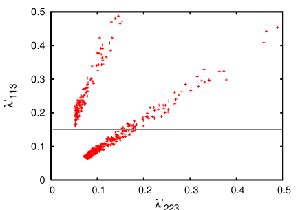
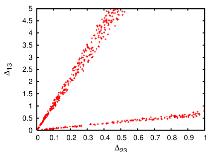
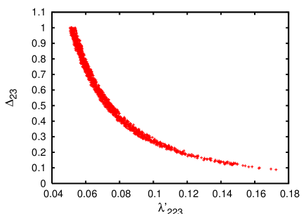
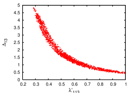
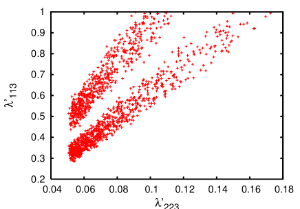
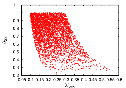
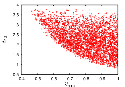
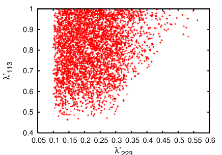
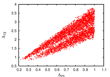
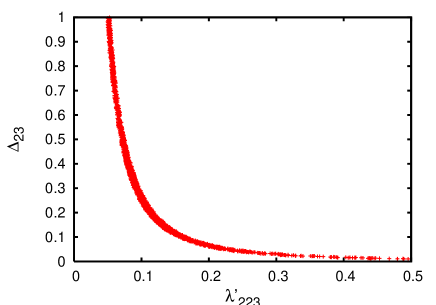
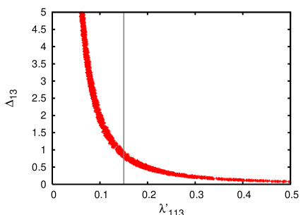
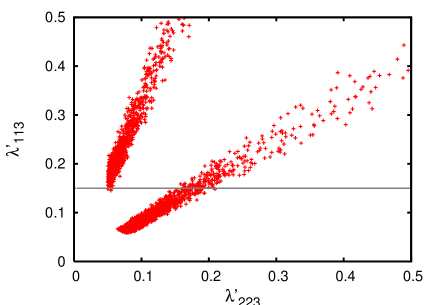
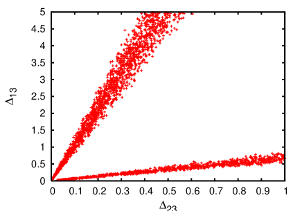
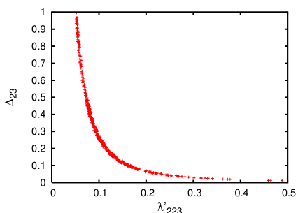
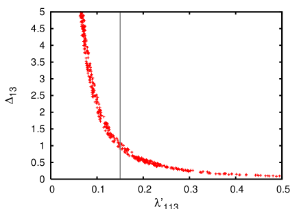
As a result of varying all the parameters, there are six possible projections of the four-dimensional scatter plot. In figures 4-7, we show four of them, the other two not giving any independent information.

Figure 4: Correlation plots for NH case with $\theta_{13}=0$. The vertical (horizontal) line in the top right (bottom left) panel corresponds to the 99% CL upper limit on $\lambda^{\prime}_{113}$ (see text).

Figure 5: Same as in Figure 4 but for the IH scenario.

Figure 6: Same as in Figure 4 but for the DN scenario.

Figure 7: Same as in Figure 4 but for $\theta_{13}=10^{\circ}$.

The plots are drawn for (i) NH (fig. 4), (ii) IH (fig. 5), (iii) DN (fig. 6), all with $\theta_{13}=0$, and (iv) NH (fig. 7), with $\theta_{13}=10^{\circ}$. No such figures are separately shown for the IH and the DN cases, because (a) there is no appreciable difference with the corresponding $\theta_{13}=0$ case, and (b) these scenarios are in general disfavoured by the constraints on $\lambda^{\prime}_{113}$.

The scatter plots are essentially based on the fact that, corresponding to any value of one of the four aforementioned parameters, we get confined to rather narrow intervals of the remaining three, in order to satisfy the relative values of the neutrino mass matrix elements answering to the tri-bimaximal mixing pattern. Thus the scatter plots turn into correlation curves (bands) whose widths come largely from the uncertainties of the neutrino oscillation data and marginally from the uncertainties in the CKM elements.

To see the most important conclusions, let us first concentrate on fig. 4. The upper panels show the allowed regions for $\lambda^{\prime}$ versus $\Delta$; one goes up as the other goes down. Qualitatively, this can be understood from the expressions of the $M_{\nu}$ elements as given in the appendix: the product of the type $\lambda^{\prime}\lambda^{\prime}\Delta$ appears in the leading contributions. The lower left-hand panel shows the correlation between $\lambda^{\prime}_{113}$ and $\lambda^{\prime}_{223}$; taken in conjunction with the upper panels, this also tells the allowed regions of the corresponding $\Delta$s, and this fact has been confirmed in the lower right-hand panel. The upper bound on $\lambda^{\prime}_{113}$, shown by a vertical line in the upper right-hand and by a horizontal line in the lower left-hand panels, corresponds to the 99% confidence level limit from charged current universality.

It should be noted that the allowed regions for $\lambda^{\prime}_{113}$ fall outside this limit for both IH and DN cases. However, such constraint, as listed in existing literature, assumes the existence of no $\lambda$-type couplings, which can invalidate the bound but play an ineffective role in neutrino mass generation, giving contributions suppressed by light lepton masses. With these in view, we have allowed $\lambda^{\prime}_{113}$ to have values larger than the upper bound found in the literature, with the caveat that the large values may indicate the existence of additional interactions of $\lambda$-type.

The graphs clearly show that the NH scenario favours larger values of $\lambda^{\prime}_{223}$ than IH, while for $\lambda^{\prime}_{113}$ it is the other way around. This is because, in the IH case, one requires the $(1,1)$ element of $M_{\nu}$ to be of higher magnitude, and one is at a relative disadvantage in the loop contributions, since the contribution to this element is suppressed by the down quark mass. One also gets restricted to rather small values of $\lambda^{\prime}_{223}$ is this case. For the degenerate neutrino case, too, $\lambda^{\prime}_{113}$ has to be on the higher side, since the corresponding contributions do not get the advantage of heavier quark masses. This re-iterates the difficulty in reconciling the IH and DN scenarios with the constraints on $\lambda^{\prime}_{113}$, which can be bypassed through, for example, the occurrence of additional $R_{p}$ violating interactions.

While it is true that the preference of NH over IH results from the way we have selected our parameters, it should be also be noted that it is more the result of selecting three $\lambda^{\prime}$-type couplings in the range of 0.1 and two squark flavour-violating parameters $\Delta$. It is of course true that one can fit the IH and DN scenarios with a larger set of R-parity violating interactions. However, with the so-called ‘minimal’ choice, the orders of magnitudes of the loop contributions are not significantly different, so long as the $\lambda^{\prime}$-parameters are in the same range, and the squarks of different flavours (due to the different indices of these parameters) participating in the loops are in the same mass range. Naturally, the contributions will be smaller with more massive squarks; then higher values of the R-parity violating couplings than what is indicated can be accommodated. Thus, while it is not our goal to establish the preference of one scenario over the other, what we successfully show is that one can generate neutrino masses with large R-parity violating couplings, and that a pattern follows from a minimal choice, which does not necessarily depend on which three parameters are involved.

V Correlated signals: some speculations

As we have noted earlier, the small values of $\lambda^{\prime}_{223}$ and $\lambda^{\prime}_{323}$ can enhance the $D_{s}\to\mu(\tau)\nu$ branching ratio marginally. However, if one indeed entertains the possibility of some other $\lambda$-type interaction to save the IH or the DN picture, it is possible that these two couplings may become large. The lepton flavour violating (LFV) decay $\Upsilon\to\mu\tau$ is, again, only marginally enhanced, and is still well below the experimental limit. However, a positive signal in this channel would be very interesting from the neutrino perspective. The same comment applies to other LFV decays, like $D^{0}\to e\mu$, driven by $\lambda^{\prime}_{113}\lambda^{\prime}_{223}$.

One of the most interesting low-energy effects for this scenario is the change in the branching ratio of $K^{+}\to\pi^{+}\nu\bar{\nu}$. The decay, based on $s\to d\nu\bar{\nu}$, is again controlled by $\lambda^{\prime}_{113}\lambda^{\prime}_{223}$. The experimental number is $B(K^{+}\longrightarrow\pi^{+}\nu{\bar{\nu}})=(1.47^{+1.30}_{-0.89})\times 10^{-10}$ pdg , while the SM prediction is about $(0.8\pm 0.1)\times 10^{-10}$. It was pointed out in welzel that an exact upper bound is difficult to obtain considering the interplay of the SM, the $R_{p}$ conserving SUSY and the $R_{p}$ violating SUSY, but it can safely be said that with couplings of the order that we have used in this work, the $R_{p}$ violating amplitude may even be larger than the SM amplitude. In that case, this mode cannot be used as a clean channel for extracting $\sin(2\beta)$. Measurement of the said angle and a comparison with the charmonium result will again be crucial for our ansatz.

VI Summary and conclusions

We have considered scenarios where $R_{p}$ violating couplings can be large, and the neutrino mass matrix can still be generated in a manner consistent with observed results. This, we argue, can be possible if there are only a few couplings of this type, so that the combinations necessary for one-loop neutrino masses are not available. Two-loop contributions come to one’s advantage in such situations, together with the possibility of flavour violation in the sfermion mass matrices. Considering the $\lambda^{\prime}$-type couplings, we have demonstrated this; with three such couplings and two squark flavour violating parameters, the NH scenario can be reproduced, guiding one to a specific region of the parameter space. For the IH and DN cases, however, this requires the value of at least one coupling to come into conflict with observable constraints unless one postulates additional R-parity violating terms in the superpotential. Of course, there may be more than one choice of the set of R-parity violating couplings leading to two-loop neutrino masses, and the exact numerical consequences in the neutrino sector can be dependent on which $\lambda^{\prime}$-couplings actually exist.

Similar conclusions can be established if one includes the bilinear R-parity violating terms in the superpotential. One neutrino state acquires a tree-level mass in such a case, thus relaxing the constraint that seems to loom large on the parameter $\lambda^{\prime}_{113}$ as discussed above. The two remaining couplings (with values in the range 0.1-1.0) and the squark flavour violation parameters can then generate the remaining terms in the mass matrix at the two-loop level. This may make the IH and DN cases less constrained.

In conclusion, large trilinear R-parity violating interactions are not necessarily an impediment to the explanation of neutrino masses and mixing. Thus if some phenomenon observed in the laboratory points strongly towards such large interaction strength, it may still explain the neutrino sector perfectly well, provided that only a few R-parity violating interactions occur in nature with sizable strength.

ACKNOWLEDGEMENTS

We thank Abhijit Bandyopadhyay and Sourov Roy for helpful discussions. AK is supported by Project No. 2007/37/9/BRNS of DAE, Government of India. The work of PD, BM and SN was partially supported by funding available from the Department of Atomic Energy, Government of India, for the Regional Centre for Accelerator-based Particle Physics, Harish-Chandra Research Institute.

APPENDIX

The two-loop matrix elements are expressed in terms of the following variables.

$$\xi_{t}=V^{*}_{ts}V_{tb}$$ (16)

$$\xi^{\prime}_{t}=V^{*}_{td}V_{tb}$$ (17)

$$\xi_{c}=V^{*}_{cs}V_{cb}$$ (18)

$$\xi^{\prime}_{c}=V^{*}_{cd}V_{cb}$$ (19)

$$x_{i}=m^{2}_{i}/M^{2}_{W}$$ (20)

The generic loop-functions with proper arguments are listed below. There are two types of such functions, depending on whether they depend on lepton masses or not.

Functions, first set: $i=e,\mu,\tau$.

$$F_{1}(x_{t},x_{W})=\frac{3x_{t}-1}{4(x_{t}-1)}-\frac{x^{2}_{t}\log x_{t}}{2(x_{t}-1)^{2}}$$ (21)

$$F_{2}(x_{t},x_{W})=1-\frac{x_{t}\log x_{t}}{x_{t}-1}$$ (22)

$$F_{1}(x_{t},x_{W})-F_{2}(x_{t},x_{W})=\frac{x_{t}(x_{t}-2)}{2(x_{t}-1)^{2}}\log x_{t}-\frac{x_{t}-3}{4(x_{t}-1)}$$ (23)

$$F_{3}(x_{t},x_{W})=-2F_{1}(x_{t},x_{W})$$ (24)

$$F_{4}(x_{c},x_{i})=\frac{1-x_{c}+x_{c}\log x_{c}}{1-x_{c}}+\frac{x_{c}\log x_{c}-x_{c}-x_{i}\log x_{i}+x_{i}}{x_{c}-x_{i}}$$ (25)

$$F_{5}(x_{c},x_{i}) = -\frac{1}{(x_{c}-x_{W})^{2}}\Big{[}\frac{1}{2}x^{2}_{c}\log x_{c}-\frac{1}{4}x^{2}_{c}-x_{w}x_{c}\log x_{c}+x_{w}x_{c}$$ (26)

$$+\frac{1}{2}x^{2}_{W}\log x_{W}-\frac{3}{4}x^{2}_{W}\Big{]}+(x_{W}\leftrightarrow x_{i})$$

$$F_{6}(x_{c},x_{i})=\frac{1}{(x_{w}-x_{c})}\Big{[}\frac{1}{2}x^{2}_{w}\log x_{w}-\frac{1}{4}x^{2}_{w}-\frac{1}{2}x^{2}_{c}\log x_{c}-\frac{1}{4}x^{2}_{c}\Big{]}$$

$$-(x_{W}\leftrightarrow x_{i})$$ (27)

$$F_{7}(x_{c},x_{i}) = \frac{1}{(x_{w}-x_{c})^{3}}\Big{[}\big{(}\frac{1}{3}x^{3}_{w}-x^{2}_{w}x_{c}+x_{w}x^{2}_{c}\big{)}\log x_{w}$$ (28)

$$-\big{(}\frac{1}{9}x^{3}_{w}-\frac{1}{2}x^{2}_{w}x_{c}+x_{w}x^{2}_{c}\big{)}-\frac{1}{3}x^{3}_{c}\log x_{c}-\frac{11}{18}x^{3}_{c}\Big{]}-(x_{W}\leftrightarrow x_{i})$$

Functions, second set:

$$F_{8}(x_{\tilde{q}},x_{b})=\frac{1}{x_{\tilde{q}}-x_{b}}-\frac{x_{b}(\log x_{\tilde{q}}-\log x_{b})}{(x_{\tilde{q}}-x_{b})^{2}}$$ (29)

$$F_{9}(x_{\tilde{q}},x_{b})=\frac{4}{(x_{\tilde{q}}-x_{b})^{2}}\left[\frac{1}{2}x^{2}_{\tilde{q}}\log x_{\tilde{q}}-\frac{1}{4}x^{2}_{\tilde{q}}-x_{\tilde{q}}x_{b}\log x_{\tilde{q}}+x_{\tilde{q}}x_{b}+\frac{1}{2}x^{2}_{b}\log x_{b}-\frac{3}{4}x^{2}_{b}\right]$$ (30)

$$F_{10}(x_{\tilde{q}},x_{b},x_{s})=F_{9}(x_{\tilde{q}},x_{b})-F_{9}(x_{\tilde{q}},x_{s})$$ (31)

$$F_{11}(x_{\tilde{q}},x_{b},x_{s})=F_{6}(x_{\tilde{q}},x_{b})-F_{6}(x_{\tilde{q}},x_{s})$$ (32)

$$F_{12}(x_{\tilde{q}},x_{b})=\frac{\log x_{\tilde{q}}-\log x_{b}}{x_{\tilde{q}}-x_{b}}$$ (33)

$$F_{13}(x_{\tilde{q}},x_{b})=\frac{1}{(x_{\tilde{q}}-x_{b})}\Big{[}\frac{1}{2}x^{2}_{\tilde{q}}\log x_{\tilde{q}}-\frac{1}{4}x^{2}_{\tilde{q}}-\frac{1}{2}x^{2}_{b}\log x_{b}+\frac{1}{4}x^{2}_{b}\Big{]}$$ (34)

Matrix element $M_{\nu}(1,1)$:

$M_{\nu}(1,1)$: Diagram 2(a) with $\phi$

$$\lambda^{\prime}_{113}\lambda^{\prime}_{113}~{}\frac{g^{2}}{4M^{2}_{W}}~{}\frac{1}{(16\pi^{2})^{2}}~{}\xi^{\prime}_{t}~{}M_{susy}~{}\frac{m_{b}m_{d}}{m^{2}_{d}-m^{2}_{b}}~{}\tilde{\Delta}_{13}\Big{[}m^{2}_{t}(F_{1}-F_{2})F_{10}(x_{\tilde{q}},x_{b},x_{d})$$

$$-m^{2}_{t}x_{d}F_{2}F_{11}(x_{\tilde{q}},x_{b},x_{d})+m^{2}_{d}F_{1}F_{10}(x_{\tilde{q}},x_{b},x_{d})\Big{]}$$ (35)

$M_{\nu}(1,1)$: Diagram 2(a) with $W$

$$\lambda^{\prime}_{113}\lambda^{\prime}_{113}~{}\frac{g^{2}}{4}~{}\frac{1}{(16\pi^{2})^{2}}~{}M_{susy}~{}\frac{m_{b}m_{d}}{m^{2}_{d}-m^{2}_{b}}~{}\tilde{\Delta}_{13}\Big{[}\xi^{\prime}_{t}[F_{3}(x_{t},x_{W})-F_{3}(x_{u},x_{W})]$$

$$+\xi^{\prime}_{c}[F_{3}(x_{c},x_{W})-F_{3}(x_{u},x_{W})]\Big{]}F_{10}(x_{\tilde{q}},x_{b},x_{d})$$ (36)

$M_{\nu}(1,1)$: Diagram 2(b) with $\phi$

$$\lambda^{\prime}_{113}\lambda^{\prime}_{113}~{}\frac{g^{2}}{4M^{2}_{W}}~{}\frac{1}{(16\pi^{2})^{2}}~{}V_{ub}~{}M_{susy}~{}{m_{b}m_{d}}~{}\tilde{\Delta}_{13}\Big{[}\frac{m^{2}_{e}}{M^{2}_{W}-m^{2}_{e}}[x_{u}F_{4}(x_{u},x_{e})F_{8}(x_{\tilde{q}},x_{b})$$

$$-F_{4}(x_{u},x_{e})F_{9}(x_{\tilde{q}},x_{b})-F_{5}(x_{u},x_{e})F_{9}(x_{\tilde{q}},x_{b})]\Big{]}$$ (37)

$M_{\nu}(1,1)$: Diagram 2(c) with $\phi$

$$\lambda^{\prime}_{113}\lambda^{\prime}_{113}~{}g^{2}\frac{1}{(16\pi^{2})^{2}}~{}V^{*}_{ud}\Big{[}\frac{x_{u}-x_{d}}{x_{w}-x_{e}}m_{e}F_{5}(x_{u},x_{e})F_{13}(x_{\tilde{q}},x_{d})$$

$$+\frac{x_{d}}{x_{w}-x_{e}}m_{e}[F_{7}(x_{u},x_{e})F_{13}(x_{\tilde{q}},x_{d})-F_{6}(x_{u},x_{e})F_{12}(x_{\tilde{q}},x_{d})]\Big{]}$$ (38)

Matrix element $M_{\nu}(2,2)$:

$M_{\nu}(2,2)$: Diagram 2(a) with $\phi$

$$\lambda^{\prime}_{223}\lambda^{\prime}_{223}~{}\frac{g^{2}}{4M^{2}_{W}}~{}\frac{1}{(16\pi^{2})^{2}}~{}\xi_{t}~{}M_{susy}~{}\frac{m_{b}m_{s}}{m^{2}_{s}-m^{2}_{b}}~{}\tilde{\Delta}_{23}\Big{[}m^{2}_{t}(F_{1}-F_{2})F_{10}(x_{\tilde{q}},x_{b},x_{s})$$

$$-m^{2}_{t}x_{s}F_{2}F_{11}(x_{\tilde{q}},x_{b},x_{s})+m^{2}_{s}F_{1}F_{10}(x_{\tilde{q}},x_{b},x_{s})\Big{]}$$ (39)

$M_{\nu}(2,2)$: Diagram 2(a) with $W$

$$\lambda^{\prime}_{223}\lambda^{\prime}_{223}~{}\frac{g^{2}}{4}~{}\frac{1}{(16\pi^{2})^{2}}~{}M_{susy}~{}\frac{m_{b}m_{s}}{m^{2}_{s}-m^{2}_{b}}~{}\tilde{\Delta}_{23}\Big{[}\xi_{t}[F_{3}(x_{t},x_{W})-F_{3}(x_{u},x_{W})]$$

$$+\xi_{c}[F_{3}(x_{c},x_{W})-F_{3}(x_{u},x_{W})]\Big{]}F_{10}(x_{\tilde{q}},x_{b},x_{s})$$ (40)

$M_{\nu}(2,2)$: Diagram 2(b) with $\phi$

$$\lambda^{\prime}_{223}\lambda^{\prime}_{223}~{}\frac{g^{2}}{4M^{2}_{W}}~{}\frac{1}{(16\pi^{2})^{2}}~{}V_{cb}~{}M_{susy}~{}{m_{b}m_{s}}~{}\tilde{\Delta}_{23}\Big{[}\frac{m^{2}_{\mu}}{M^{2}_{W}-m^{2}_{\mu}}[x_{c}F_{4}(x_{c},x_{\mu})F_{6}(x_{\tilde{q}},x_{b})$$

$$-F_{4}(x_{c},x_{\mu})F_{9}(x_{\tilde{q}},x_{b})-F_{5}(x_{c},x_{\mu})F_{9}(x_{\tilde{q}},x_{b})]\Big{]}$$ (41)

$M_{\nu}(2,2)$: Diagram 2(c) with $\phi$

$$\lambda^{\prime}_{223}\lambda^{\prime}_{223}~{}g^{2}\frac{1}{(16\pi^{2})^{2}}~{}V^{*}_{cs}\Big{[}\frac{x_{c}-x_{s}}{x_{w}-x_{\mu}}m_{\mu}F_{5}(x_{c},x_{\mu})F_{13}(x_{\tilde{q}},x_{s})$$

$$+\frac{x_{s}}{x_{w}-x_{\mu}}m_{\mu}[F_{7}(x_{c},x_{\mu})F_{13}(x_{\tilde{q}},x_{s})-F_{6}(x_{c},x_{\mu})F_{12}(x_{\tilde{q}},x_{s})]\Big{]}$$ (42)

Matrix element $M_{\nu}(3,3)$ same as $M_{\nu}(2,2)$ with $\mu$ replaced by $\tau$.

Matrix element $M_{\nu}(1,2)=M_{\nu}(2,1)$:

$M_{\nu}(1,2)$: Diagram 2(a) with $\phi$

$$\lambda^{\prime}_{113}\lambda^{\prime}_{223}~{}\frac{g^{2}}{8M^{2}_{W}}~{}\frac{1}{(16\pi^{2})^{2}}~{}M_{susy}\Big{(}\Big{[}\xi_{t}~{}\frac{m_{b}m_{d}}{m^{2}_{s}-m^{2}_{b}}~{}\tilde{\Delta}_{13}\Big{]}\Big{[}m^{2}_{t}(F_{1}-F_{2})F_{10}(x_{\tilde{q}},x_{b},x_{s})$$

$$-m^{2}_{t}x_{s}F_{2}F_{11}(x_{\tilde{q}},x_{b},x_{s})+m^{2}_{s}F_{1}F_{10}(x_{\tilde{q}},x_{b},x_{s})\Big{]}$$

$$+\Big{[}\xi^{\prime}_{t}~{}\frac{m_{b}m_{s}}{m^{2}_{d}-m^{2}_{b}}~{}\tilde{\Delta}_{23}\Big{]}\Big{[}m^{2}_{t}(F_{1}-F_{2})F_{10}(x_{\tilde{q}},x_{b},x_{d})$$

$$-m^{2}_{t}x_{d}F_{2}F_{11}(x_{\tilde{q}},x_{b},x_{d})+m^{2}_{d}F_{1}F_{10}(x_{\tilde{q}},x_{b},x_{d})\Big{]}\Big{)}$$ (43)

$M_{\nu}(1,2)$: Diagram 2(a) with $W$

$$\lambda^{\prime}_{113}\lambda^{\prime}_{223}~{}\frac{g^{2}}{8}~{}\frac{1}{(16\pi^{2})^{2}}~{}M_{susy}\Big{(}\Big{[}\frac{m_{b}m_{d}}{m^{2}_{s}-m^{2}_{b}}~{}\tilde{\Delta}_{13}\Big{]}\Big{[}\xi_{t}[F_{3}(x_{t},x_{W})-F_{3}(x_{u},x_{W})]$$

$$+\xi_{c}[F_{3}(x_{c},x_{W})-F_{3}(x_{u},x_{W})]\Big{]}F_{10}(x_{\tilde{q}},x_{b},x_{s})+\Big{[}\frac{m_{b}m_{s}}{m^{2}_{d}-m^{2}_{b}}~{}\tilde{\Delta}_{23}\Big{]}\Big{[}\xi^{\prime}_{t}[F_{3}(x_{t},x_{W})$$

$$-F_{3}(x_{u},x_{W})]+\xi^{\prime}_{c}[F_{3}(x_{c},x_{W})-F_{3}(x_{u},x_{W})]\Big{]}F_{10}(x_{\tilde{q}},x_{b},x_{d})\Big{)}$$ (44)

$M_{\nu}(1,2)$: Diagram 2(b) with $\phi$

$$\lambda^{\prime}_{113}\lambda^{\prime}_{223}~{}\frac{g^{2}}{8M^{2}_{W}}~{}\frac{1}{(16\pi^{2})^{2}}~{}M_{susy}\Big{(}\Big{[}V_{cb}~{}{m_{b}m_{d}}~{}\tilde{\Delta}_{13}\Big{]}\Big{[}\frac{m^{2}_{\mu}}{M^{2}_{W}-m^{2}_{\mu}}[x_{c}F_{4}(x_{c},x_{\mu})F_{8}(x_{\tilde{q}},x_{b})$$

$$-F_{4}(x_{c},x_{\mu})F_{9}(x_{\tilde{q}},x_{b})-F_{5}(x_{c},x_{\mu})F_{9}(x_{\tilde{q}},x_{b})]\Big{]}+\Big{[}V_{ub}~{}{m_{b}m_{s}}~{}\tilde{\Delta}_{23}\Big{]}$$

$$\Big{[}\frac{m^{2}_{e}}{M^{2}_{W}-m^{2}_{e}}[x_{u}F_{4}(x_{u},x_{e})F_{8}(x_{\tilde{q}},x_{b})-F_{4}(x_{u},x_{e})F_{9}(x_{\tilde{q}},x_{b})-F_{5}(x_{u},x_{e})F_{9}(x_{\tilde{q}},x_{b})]\Big{]}\Big{)}$$ (45)

$M_{\nu}(1,2)$: Diagram 2(c) with $\phi$

$$\lambda^{\prime}_{113}\lambda^{\prime}_{223}~{}g^{2}\frac{1}{(16\pi^{2})^{2}}\Big{[}V^{*}_{cs}\Big{(}\frac{x_{c}-x_{s}}{x_{w}-x_{\mu}}m_{\mu}F_{5}(x_{c},x_{\mu})F_{13}(x_{\tilde{q}},x_{s})$$

$$+\frac{x_{s}}{x_{w}-x_{\mu}}m_{\mu}[F_{7}(x_{c},x_{\mu})F_{13}(x_{\tilde{q}},x_{s})-F_{6}(x_{c},x_{\mu})F_{12}(x_{\tilde{q}},x_{s})]\Big{)}+$$

$$V^{*}_{ud}\Big{(}\frac{x_{u}-x_{d}}{x_{w}-x_{e}}m_{e}F_{5}(x_{u},x_{e})F_{13}(x_{\tilde{q}},x_{d})$$

$$+\frac{x_{d}}{x_{w}-x_{e}}m_{e}[F_{7}(x_{u},x_{e})F_{13}(x_{\tilde{q}},x_{d})-F_{6}(x_{u},x_{e})F_{12}(x_{\tilde{q}},x_{d})]\Big{)}\Big{]}$$ (46)

Matrix elements $M_{\nu}(1,3)$ and $M_{\nu}(3,1)$ are same as $M_{\nu}(1,2)$ with $\mu$ replaced by $\tau$.

Matrix element $M_{\nu}(2,3)=M_{\nu}(3,2)$:

$M_{\nu}(2,3)$: Diagram 2(a) with $\phi$

$$\lambda^{\prime}_{223}\lambda^{\prime}_{323}~{}\frac{g^{2}}{8M^{2}_{W}}~{}\frac{1}{(16\pi^{2})^{2}}~{}\xi_{t}~{}M_{susy}~{}\frac{m_{b}m_{s}}{m^{2}_{s}-m^{2}_{b}}~{}\tilde{\Delta}_{23}\Big{[}m^{2}_{t}(F_{1}-F_{2})F_{10}(x_{\tilde{q}},x_{b},x_{s})$$

$$-m^{2}_{t}x_{s}F_{2}F_{11}(x_{\tilde{q}},x_{b},x_{s})+m^{2}_{s}F_{1}F_{10}(x_{\tilde{q}},x_{b},x_{s})\Big{]}$$ (47)

$M_{\nu}(2,3)$: Diagram 2(a) with $W$

$$\lambda^{\prime}_{223}\lambda^{\prime}_{323}~{}\frac{g^{2}}{8}~{}\frac{1}{(16\pi^{2})^{2}}~{}M_{susy}~{}\frac{m_{b}m_{s}}{m^{2}_{s}-m^{2}_{b}}~{}\tilde{\Delta}_{23}\Big{[}\xi_{t}[F_{3}(x_{t},x_{W})-F_{3}(x_{u},x_{W})]$$

$$+\xi_{c}[F_{3}(x_{c},x_{W})-F_{3}(x_{u},x_{W})]\Big{]}F_{10}(x_{\tilde{q}},x_{b},x_{s})$$ (48)

$M_{\nu}(2,3)$: Diagram 2(b) with $\phi$

$$\lambda^{\prime}_{223}\lambda^{\prime}_{323}~{}\frac{g^{2}}{8M^{2}_{W}}~{}\frac{1}{(16\pi^{2})^{2}}~{}V_{cb}~{}M_{susy}~{}{m_{b}m_{s}}~{}\tilde{\Delta}_{23}\Big{[}\frac{m^{2}_{\mu}}{M^{2}_{W}-m^{2}_{\mu}}~{}[x_{c}F_{4}(x_{c},x_{\mu})F_{8}(x_{\tilde{q}},x_{b})$$

$$-F_{4}(x_{c},x_{\mu})F_{9}(x_{\tilde{q}},x_{b})-F_{5}(x_{c},x_{\mu})F_{9}(x_{\tilde{q}},x_{b})]+\frac{m^{2}_{\tau}}{M^{2}_{W}-m^{2}_{\tau}}~{}[x_{c}F_{4}(x_{c},x_{\tau})F_{8}(x_{\tilde{q}},x_{b})$$

$$-F_{4}(x_{c},x_{\tau})F_{9}(x_{\tilde{q}},x_{b})-F_{5}(x_{c},x_{\tau})F_{9}(x_{\tilde{q}},x_{b})]\Big{]}$$ (49)

$M_{\nu}(2,3)$: Diagram 2(c) with $\phi$

$$\lambda^{\prime}_{223}\lambda^{\prime}_{323}~{}g^{2}\frac{1}{(16\pi^{2})^{2}}~{}V^{*}_{cb}\Big{[}\Big{(}\frac{x_{c}-x_{s}}{x_{w}-x_{\mu}}m_{\mu}F_{5}(x_{c},x_{\mu})F_{13}(x_{\tilde{q}},x_{s})$$

$$+\frac{x_{s}}{x_{w}-x_{\mu}}m_{\mu}[F_{7}(x_{c},x_{\mu})F_{13}(x_{\tilde{q}},x_{s})-F_{6}(x_{c},x_{\mu})F_{12}(x_{\tilde{q}},x_{s})]\Big{)}$$

$$+\Big{(}\frac{x_{c}-x_{s}}{x_{w}-x_{\tau}}m_{\tau}F_{5}(x_{c},x_{\tau})F_{13}(x_{\tilde{q}},x_{s})$$

$$+\frac{x_{s}}{x_{w}-x_{\tau}}m_{\tau}[F_{7}(x_{c},x_{\tau})F_{13}(x_{\tilde{q}},x_{s})-F_{6}(x_{c},x_{\tau})F_{12}(x_{\tilde{q}},x_{s})]\Big{)}\Big{]}$$ (50)

References

• (1) Q. R. Ahmad et al. [SNO Collaboration], Phys. Rev. Lett.  87, 071301 (2001) [arXiv:nucl-ex/0106015]; Q. R. Ahmad et al. [SNO Collaboration], Phys. Rev. Lett.  89, 011301 (2002) [arXiv:nucl-ex/0204008]; Q. R. Ahmad et al. [SNO Collaboration], Phys. Rev. Lett.  89, 011302 (2002) [arXiv:nucl-ex/0204009].
• (2) A. Bandyopadhyay, S. Choubey, S. Goswami and K. Kar, Phys. Lett.  B 519, 83 (2001) [arXiv:hep-ph/0106264]; M. V. Garzelli and C. Giunti, JHEP 0112, 017 (2001) [arXiv:hep-ph/0108191]; J. N. Bahcall, M. C. Gonzalez-Garcia and C. Pena-Garay, JHEP 0108, 014 (2001) [arXiv:hep-ph/0106258]; G. L. Fogli, E. Lisi, D. Montanino and A. Palazzo, Phys. Rev.  D 64, 093007 (2001) [arXiv:hep-ph/0106247]; P. I. Krastev and A. Y. Smirnov, Phys. Rev.  D 65, 073022 (2002) [arXiv:hep-ph/0108177]; A. Bandyopadhyay, S. Choubey, S. Goswami and D. P. Roy, Phys. Lett.  B 540, 14 (2002) [arXiv:hep-ph/0204286].
• (3) K. Eguchi et al. [KamLAND Collaboration], Phys. Rev. Lett.  90, 021802 (2003) [arXiv:hep-ex/0212021].
• (4) G. R. Farrar and P. Fayet, Phys. Lett.  B 76, 575 (1978); C. S. Aulakh and R. N. Mohapatra, Phys. Lett.  B 119, 136 (1982); L. J. Hall and M. Suzuki, Nucl. Phys.  B 231, 419 (1984); J. R. Ellis, G. Gelmini, C. Jarlskog, G. G. Ross and J. W. F. Valle, Phys. Lett.  B 150, 142 (1985); G. G. Ross and J. W. F. Valle, Phys. Lett.  B 151, 375 (1985); S. Dawson, Nucl. Phys.  B 261, 297 (1985); R. Barbieri and A. Masiero, Nucl. Phys.  B 267, 679 (1986).
• (5) S. Dimopoulos and L. J. Hall, Phys. Lett.  B 196 (1987) 135; R. M. Godbole, P. Roy and X. Tata, Nucl. Phys. B401, (1993) 67. R. M. Godbole, P. Roy and X. Tata, Nucl. Phys.  B 401, 67 (1993) [arXiv:hep-ph/9209251].
• (6) B. C. Allanach, A. Dedes and H. K. Dreiner, Phys. Rev.  D 60, 056002 (1999) [arXiv:hep-ph/9902251]; Phys. Rev.  D 69, 115002 (2004) [Erratum-ibid.  D 72, 079902 (2005)] [arXiv:hep-ph/0309196].
• (7) See, for example, H. K. Dreiner, arXiv:hep-ph/9707435; G. Bhattacharyya, arXiv:hep-ph/9709395; R. Barbier et al., arXiv:hep-ph/9810232; S. Rakshit, G. Bhattacharyya and A. Raychaudhuri, Phys. Rev.  D 59, 091701 (1999) [arXiv:hep-ph/9811500]; B. Mukhopadhyaya, arXiv:hep-ph/0301278.
• (8) M. Drees, S. Pakvasa, X. Tata and T. ter Veldhuis, Phys. Rev.  D 57, 5335 (1998) [arXiv:hep-ph/9712392]; E. J. Chun, S. K. Kang, C. W. Kim and U. W. Lee, Nucl. Phys.  B 544, 89 (1999) [arXiv:hep-ph/9807327].
• (9) F. Borzumati and J. S. Lee, Phys. Rev.  D 66, 115012 (2002) [arXiv:hep-ph/0207184].
• (10) J. S. Hagelin, S. Kelley and T. Tanaka, Nucl. Phys.  B 415, 293 (1994); S. Bertolini, F. Borzumati, A. Masiero and G. Ridolfi, Nucl. Phys.  B 353, 591 (1991); F. Gabbiani, E. Gabrielli, A. Masiero and L. Silvestrini, Nucl. Phys.  B 477, 321 (1996) [arXiv:hep-ph/9604387].
• (11) A. Kundu and S. Nandi, Phys. Rev.  D 78, 015009 (2008) [arXiv:0803.1898 [hep-ph]].
• (12) B. A. Dobrescu and A. S. Kronfeld, Phys. Rev. Lett.  100, 241802 (2008) [arXiv:0803.0512 [hep-ph]].
• (13) C. Amsler et al. [Particle Data Group], Phys. Lett.  B 667, 1 (2008); B. Aubert et al. [BABAR Collaboration], Phys. Rev. Lett.  98, 141801 (2007) [arXiv:hep-ex/0607094]; T. K. Pedlar et al. [CLEO Collaboration], Phys. Rev.  D 76, 072002 (2007) [arXiv:0704.0437 [hep-ex]]; K. M. Ecklund et al. [CLEO Collaboration], Phys. Rev. Lett.  100, 161801 (2008) [arXiv:0712.1175 [hep-ex]]; K. Abe et al. [Belle Collaboration], Phys. Rev. Lett.  100, 241801 (2008) [arXiv:0709.1340 [hep-ex]].
• (14) E. Follana, C. T. H. Davies, G. P. Lepage and J. Shigemitsu [HPQCD Collaboration and UKQCD Collaboration], Phys. Rev. Lett.  100, 062002 (2008) [arXiv:0706.1726 [hep-lat]].
• (15) V. Lubicz and C. Tarantino, arXiv:0807.4605 [hep-lat];
• (16) See Ref. 1 of dsdata .
• (17) P. F. Harrison, D. H. Perkins and W. G. Scott, Phys. Lett.  B 530, 167 (2002) [arXiv:hep-ph/0202074].
• (18) A. Bandyopadhyay, S. Choubey, S. Goswami, S. T. Petcov and D. P. Roy, arXiv:0804.4857 [hep-ph].
• (19) V. D. Barger, G. F. Giudice and T. Han, Phys. Rev.  D 40, 2987 (1989).
• (20) W. Love et al. [CLEO Collaboration], arXiv:0807.2695 [hep-ex].
• (21) B. de Carlos and P. L. White, Phys. Rev.  D 55, 4222 (1997) [arXiv:hep-ph/9609443].
• (22) J. Welzel, arXiv:hep-ph/0505094.
• (23) S. Roy and B. Mukhopadhyaya, Phys. Rev.  D 55, 7020 (1997) [arXiv:hep-ph/9612447]; B. Mukhopadhyaya, S. Roy and F. Vissani, Phys. Lett.  B 443, 191 (1998) [arXiv:hep-ph/9808265]; M. Hirsch, M. A. Diaz, W. Porod, J. C. Romao and J. W. F. Valle, Phys. Rev.  D 62, 113008 (2000) [Erratum-ibid.  D 65, 119901 (2002)] [arXiv:hep-ph/0004115]; A. S. Joshipura, R. D. Vaidya and S. K. Vempati, Nucl. Phys.  B 639, 290 (2002) [arXiv:hep-ph/0203182]; A. Abada, G. Bhattacharyya and M. Losada, Phys. Rev.  D 66, 071701 (2002) [arXiv:hep-ph/0208009].