The Quantum State of Inflationary Perturbations

Abstract

This article reviews the properties of the quantum state of inflationary perturbations. After a brief description of the inflationary background, the wavefunction of the Mukhanov-Sasaki variable is calculated and shown to be that of a strongly squeezed state. The corresponding Wigner function and density matrix, which are convenient tools to characterize the properties of a quantum state, are also evaluated. Finally, the issue of definite outcomes for inflation is discussed.

1 Introduction

According to the theory of inflation, the very early universe underwent a period of quasi-exponential expansion [1, 2, 3, 4, 5]. Such a phase of evolution can arise in general relativity when the pressure of the fluid sourcing the Einstein equations is negative. This is the case if a scalar field with a flat potential dominated in the very early universe. This simple assumption, which solely rests on classical physics, is quite remarkable as it allows us to solve many puzzles of the former standard model of cosmology, i.e. the hot Big Bang scenario.

But even more interesting results can be obtained when quantum effects are taken into account. In particular, considering small inhomogeneous fluctuations on top of an isotropic and homogeneous expanding background and quantizing them gives a very elegant explanation for the origin of the Cosmic Microwave Background (CMB) anisotropies and of the large scale structures [6, 7, 8, 9, 10, 11] (for reviews, see Refs. [12, 13, 14, 15, 16, 17, 18]). As is well-known, this leads to an almost scale-invariant power spectrum for the cosmological perturbations [19], the small deviations from scale invariance being connected to the detailed shape of the scalar field potential. As a consequence, this provides a method to constrain the physical conditions that prevailed when the universe was very young, at energy scales that can be as high as $10^{15}\mbox{GeV}$ [20, 21, 22, 23, 24, 25, 26].

This is not, however, the only interesting aspect that arises when quantum effects are included into the inflationary picture. Very fundamental questions, connected to the quantum nature of the gravitational field and/or to the foundations of quantum mechanics, can also be discussed in this framework. In these proceedings, we review the properties of the quantum state of inflationary perturbations [27, 28] and briefly discuss how it is related to the more fundamental issues mentioned above [27, 28, 29, 30, 31, 32, 33, 34, 35, 36, 37, 38]. This short article is organized as follows. In the next section, Sec. 2, we describe inflation at the background level. Then, in Sec. 3, we review the theory of inflationary fluctuations of quantum-mechanical origin, paying special attention to the quantum state in which the perturbations are placed. Finally, in Sec. 4, we present our conclusions and briefly mention and discuss the open issues.

2 The Inflationary Background

Inflation is a phase of accelerated, quasi-exponential, expansion that took place in the very early Universe, prior to the standard hot Big-Bang phase  [1, 2, 3, 4, 5] (for reviews, see Refs. [13, 14, 15]). It is important to realize that inflation does not replace the former cosmological standard model by a new one but just completes it. Postulating such a phase of evolution allows us to solve the standard problems of the hot Big-Bang model. Given that, at very high energies, field theory is the relevant framework to describe matter, a natural way to realize inflation is to consider that a real scalar field (the “inflaton” field) was the dominant source of energy density in the early Universe (there also exist versions of the inflationary scenario where inflation is driven by several scalar fields). This assumption is moreover compatible with the observed homogeneity, isotropy and flatness of the early Universe. Technically, this can be described by the metric tensor ${\rm d}s^{2}=-{\rm d}t^{2}+a^{2}(t)\delta_{ij}{\rm d}x^{i}{\rm d}x^{j}$, where $a(t)$ is the Friedman-Lemaître-Robertson-Walker (FLRW) scale factor and $t$ the cosmic time. The Einstein equations imply that $\ddot{a}/a=-(\rho+3p)/(6M_{{}_{\mathrm{Pl}}}^{2})$, $\rho$ and $p$ being the energy density and pressure of the matter sourcing the gravitational field and $M_{{}_{\mathrm{Pl}}}$ the Planck mass (a dot denotes a derivative with respect to the cosmic time $t$). For a scalar field, this reduces to $\ddot{a}/a=V(\varphi)(1-\dot{\varphi}^{2}/V)/(3M_{{}_{\mathrm{Pl}}}^{2})$, where $V(\varphi)$ is the scalar field potential. This means that inflation (i.e. $\ddot{a}>0$) can be obtained provided the inflaton slowly rolls down its potential so that its potential energy dominates over its kinetic energy. This also shows that the inflaton potential must be sufficiently flat, a requirement which is not always easy to obtain in realistic theories and makes the inflationary model building problem a difficult issue [39]. The physical nature of the inflaton field has not been identified (there are many candidates) and, as a consequence, the shape of $V(\varphi)$ is not known. Of course, different $V(\varphi)$ lead to different inflationary expansions but, since these different potentials must all be sufficiently flat, the corresponding scale factors are all approximately given by the de Sitter solution. This solution is described by the scale factor $a(t)\simeq{\rm e}^{Ht}$, where $H\equiv\dot{a}/a$ is the Hubble parameter, a slowly-varying quantity directly related to the energy scale of inflation. Observationally, this latter quantity is not known but is constrained  [22] to be between the Grand Unified Theory (GUT) scale, that is to say $\sim 10^{15}\,\mbox{GeV}$, and $\sim 1\,\mbox{TeV}$. It is also interesting to remark that the energy density during inflation, $\rho_{\rm inf}\simeq 3H^{2}_{\rm inf}M_{{}_{\mathrm{Pl}}}^{2}$, remains approximately constant. This implies the remarkable property that the classical background approximation remains valid even if one runs the clock backwards and study the initial stages of inflation. This would no longer be the case if an ordinary fluid (e.g. radiation or matter) dominated the energy budget of the early Universe since the scaling $\rho\propto 1/a^{4}$ or $\rho\propto 1/a^{3}$ would quickly imply that $\rho\gg M_{{}_{\mathrm{Pl}}}^{4}$ at early times. Of course, this does not mean that quantum effects play no role during inflation. As a matter of fact, when the quantum kicks $\Delta\varphi_{\rm q}$ are much larger than the typical classical motion $\Delta\varphi_{\rm cl}\simeq V^{\prime}/(3H^{2})$, they must be taken into account. This can be done in the framework of stochastic inflation [40, 41].

But the arguably most impressive result coming from including the quantum effects into the inflationary picture concerns the origin of the cosmological fluctuations that give rise to the Cosmic Microwave Background (CMB) anisotropies and to the large-scale structures. We turn to this question in the next section.

3 Inflationary Perturbations

According to inflation, the seeds of cosmological fluctuations are the quantum fluctuations of the inflaton and gravitational fields. As is well-known, this idea leads to predictions that are in remarkable agreement with astrophysical data [20, 21, 22, 23, 24, 25, 26]. From the theoretical point of view, the perturbations are viewed as small ripples on top of a classical background in close analogy with the condensed matter situation where phonons are considered to be quantized excitations propagating within a classical crystal. In order to describe cosmological perturbations, one has to go beyond the homogeneity and isotropy of the FRLW metric. This can be accomplished by writing the metric as [12] $\mathrm{d}s^{2}=a^{2}\left(\eta\right)\Bigl{\{}-\left(1-2\phi\right)\mathrm{d}\eta^{2}+2\left(\partial_{i}B\right)\mathrm{d}x^{i}\mathrm{d}\eta+\left[\left(1-2\psi\right)\delta_{ij}+2\partial_{i}\partial_{j}E\right]\mathrm{d}x^{i}\mathrm{d}x^{j}\Bigr{\}}$, where $\eta$ is the conformal time and where the four functions $\phi$, $B$, $\psi$ and $E$ are functions of time and space. The above approach is, however, redundant because of gauge freedom [12, 42, 43]. The gravitational sector can in fact be described by a single, gauge-invariant, quantity, the so-called Bardeen potential $\Phi_{{}_{\rm B}}$ defined by [42] $\Phi_{{}_{\rm B}}\left(\eta,\bm{x}\right)=\phi+\left[a\left(B-E^{\prime}\right)\right]^{\prime}/a,$ where a prime denotes a derivative with respect to the conformal time $\eta$. In the same manner, the matter sector can be modeled by the gauge invariant fluctuation of the scalar field $\delta\varphi^{\left(\mathrm{gi}\right)}\left(\eta,\bm{x}\right)=\delta\varphi+\varphi^{\prime}\left(B-E^{\prime}\right)$. The two quantities $\Phi_{{}_{\rm B}}$ and $\delta\varphi^{\left(\mathrm{gi}\right)}$ are related by a perturbed Einstein constraint. This implies that the scalar sector can in fact be described by a single quantity. This quantity is the Mukhanov-Sasaki variable [6, 44] which is a combination of the Bardeen potential and of the gauge invariant field, namely $v\left(\eta,\bm{x}\right)=a\left[\delta\varphi^{\left(\mathrm{gi}\right)}+\varphi^{\prime}\Phi_{{}_{\rm B}}/\mathcal{H}\right]$, where ${\cal H}\equiv a^{\prime}/a$. It is also convenient to Fourier transform $v(\eta,{\bm{x}})$ since we consider a linear theory and, hence, all the modes evolve independently. Therefore, instead of $v(\eta,\bm{x})$, we will rather work with its Fourier amplitude $v_{\bm{k}}(\eta)$. Its equation of motion can be easily obtained from the perturbed Einstein equations and reads

$$v_{\bm{k}}^{\prime\prime}+\omega^{2}\left(\eta,\bm{k}\right)v_{\bm{k}}=0,$$ (1)

where the time-dependent frequency $\omega(\eta,\bm{k})$ can be written as $\omega^{2}\left(\eta,\bm{k}\right)=k^{2}-\left(a\sqrt{\epsilon_{1}}\right)^{\prime\prime}/(a\sqrt{\epsilon_{1}})$, $k$ being the wavenumber of the mode under consideration and $\epsilon_{1}\equiv-\dot{H}/H^{2}$ the first slow-roll parameter characterizing the cosmological expansion during inflation. The above equation is the equation of a parametric oscillator (i.e. similar to a pendulum the length of which can change with time). In the Minkowski situation, the scale factor is a constant and $\omega=k$. In this case, one deals with an harmonic oscillator. We see that the time dependence of the frequency $\omega(\eta,\bm{k})$ is entirely due to the fact that the perturbations live in a dynamical spacetime. It is worth noticing that Eq. (1) appears in other interesting physical situations such as the Schwinger effect [45, 46] or the dynamical Casimir effect [47] (recently observed for the first time in the laboratory, see Ref. [48]) and, each time, the same phenomenon is observed: particle creation under the influence of the classical, time-dependent, source even if the details of the corresponding process (number of pairs created, power spectrum etc …) depend on the precise time evolution of the source. In this sense, the theory of cosmological perturbations can be viewed as “standard” in the framework of quantum field theory. The only new aspect is that the time-dependent source is the classical gravitational background of the expanding space-time. Let us also notice that inflation is in fact not necessary in order to have particle creation: as is clear from the above considerations, only a time-dependent scale factor is necessary. However, the inflationary expansion becomes mandatory if one wants a $\omega(\eta,\bm{k})$ which leads to a power spectrum in agreement with the CMB measurements.

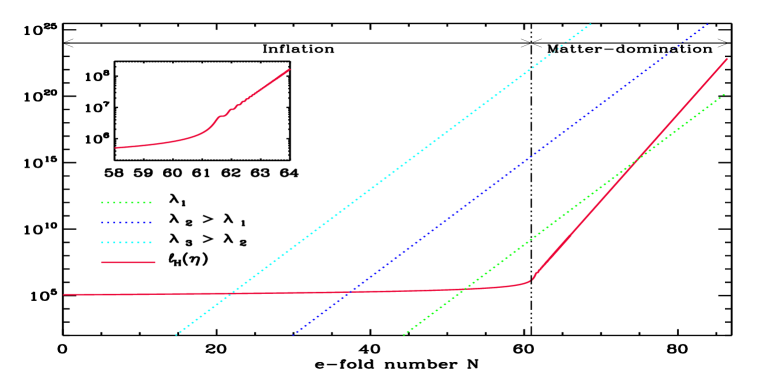
Figure 1: Evolution of various relevant length scales (in Planck units) during and after inflation. The solid red line represents the Hubble radius $\ell_{{}_{\rm H}}\equiv 1/H$. It is almost constant during inflation and starts to grow during the post-inflation era (during this phase, the inflaton field oscillates at the bottom of its potential and the universe becomes matter-dominated. Small oscillations in $\ell_{{}_{\rm H}}$ are clearly visible in the inset). The three dashed lines represent the physical wavelengths of three different Fourier modes. Initially within the Hubble radius, they exit $\ell_{{}_{\rm H}}$ during inflation and re-enter it in the post-inflationary era.

We now describe how the cosmological fluctuations are quantized. In order to achieve this goal, it is also more convenient to work with real variables. Therefore, we introduce the following definitions $v_{\bm{k}}\equiv\left(v_{\bm{k}}^{\mathrm{{\rm R}}}+iv_{\bm{k}}^{\mathrm{{\rm I}}}\right)/\sqrt{2}$ and for the conjugate momentum of the Mukhanov-Sasaki variable, $p_{\bm{k}}\equiv\left(p_{\bm{k}}^{\mathrm{{\rm R}}}+ip_{\bm{k}}^{\mathrm{{\rm I}}}\right)/\sqrt{2}$. In the Schrödinger approach, the quantum state of the system is described by a wavefunctional, $\Psi\left[v(\eta,{\bm{x}})\right]$. Since we are working in Fourier space (and since the theory is still free in the sense that it does not contain terms with power higher than two in the Lagrangian), the wavefunctional can also be factorized into mode components as

$$\Psi\left[v(\eta,{\bm{x}})\right]=\prod_{\bm{k}}\Psi_{\bm{k}}\left(v_{\bm{k}}^{\mathrm{R}},v_{\bm{k}}^{\mathrm{I}}\right)=\prod_{\bm{k}}\Psi^{\rm R}_{\bm{k}}\left(v_{\bm{k}}^{\mathrm{R}}\right)\Psi^{\rm I}_{\bm{k}}\left(v_{\bm{k}}^{\mathrm{I}}\right).$$ (2)

It can be shown that the solution to the Schrödinger equation can be written as a Gaussian function, which should not come as a surprise since we are quantizing an oscillator. Concretely, one can write

$$\Psi_{\bm{k}}^{\rm R,I}\left(\eta,v_{\bm{k}}^{\rm R,I}\right)=N_{\bm{k}}(\eta){\rm e}^{-\Omega_{\bm{k}}(\eta)\left(v_{\bm{k}}^{\rm R,I}\right)^{2}}.$$ (3)

where the functions $N_{\bm{k}}(\eta)$ and $\Omega_{\bm{k}}(\eta)$ (which do not depend on whether one considers the wavefunction of the real or imaginary parts of the Mukhanov-Sasaki variable) can be expressed as

$$\left|N_{\bm{k}}\right|=\left(\frac{2\Re\mathrm{e}\,\Omega_{\bm{k}}}{\pi}\right)^{1/4},\quad\Omega_{\bm{k}}=-\frac{i}{2}\frac{f_{\bm{k}}^{\prime}}{f_{\bm{k}}},$$ (4)

where $f_{\bm{k}}$ is a function obeying the equation $f_{\bm{k}}^{\prime\prime}+\omega^{2}f_{\bm{k}}=0$, that is to say exactly Eq. (1).

We now discuss the question of the initial conditions. The fundamental assumption of inflation is that the perturbations are initially in their ground state. At the beginning of inflation, all the modes of astrophysical interest today have a physical wavelength smaller than the Hubble radius, see Fig. 1. In this regime, each mode now behaves as a harmonic oscillator (as opposed to a parametric oscillator in the generic case) with frequency $\omega=k$. As a consequence, the differential equation for $f_{\bm{k}}(\eta)$ can easily be solved and the solution reads $f_{\bm{k}}=A_{\bm{k}}{\rm e}^{ik\eta}+B_{\bm{k}}{\rm e}^{-ik\eta}$, $A_{\bm{k}}$ and $B_{\bm{k}}$ being integration constants. Upon using the second equation (4), one has

$$\Omega_{\bm{k}}\rightarrow\frac{k}{2}\frac{A_{\bm{k}}{\rm e}^{ik\eta}-B_{\bm{k}}{\rm e}^{-ik\eta}}{A_{\bm{k}}{\rm e}^{ik\eta}+B_{\bm{k}}{\rm e}^{-ik\eta}}.$$ (5)

The wavefunction (3) represents the ground state wavefunction of a harmonic oscillator if $\Omega_{\bm{k}}=k/2$. Therefore, one must choose the initial conditions such that $B_{\bm{k}}=0$, the value of $A_{\bm{k}}$ turning out to be irrelevant in this regime. This choice of initial conditions completely determines the solution and is referred to as the Bunch-Davies vacuum [49].

We have just seen that, when the wavelength of a Fourier mode is smaller than the Hubble radius, the corresponding wavefunction can be chosen to be the ground state wavefunction of a harmonic oscillator. However, this is no longer the case when the mode exits the Hubble radius, see Fig. 1. In this regime, the function $\Omega_{\bm{k}}(\eta)$ no longer equals $k/2$ and acquires a non trivial time-dependence. In fact, a time dependent wavefunction as the one in Eq. (3) represents a very peculiar quantum state known as a squeezed state. A squeezed state is a Gaussian state for which there exists a direction in the plane $(p_{\bm{k}},v_{\bm{k}})$ where the dispersion is extremely small, i.e. exponentially small $\simeq{\rm e}^{-2r_{\bm{k}}}$ where $r_{\bm{k}}$ is the squeezing parameter (of course, the dispersion in the perpendicular direction is very large $\simeq{\rm e}^{2r_{\bm{k}}}$ in order to satisfy the Heisenberg relation). The phenomenon of squeezing is widely studied in many different branches of physics, in particular in quantum optics. Squeezing occurs each time the quantization of a parametric oscillator is carried out. It is remarkable that the quantization of small fluctuations on top of an expanding universe also leads to that phenomenon. Another interesting feature is that cosmological squeezing is much larger than what can be achieved in the laboratory [50]: for modes of cosmological interest today, $r_{\bm{k}}$ can reach values of order $\sim 10^{2}$ [27]. In the literature, this regime is very often described as a regime where the cosmological perturbations have classicalized [30, 29, 33, 33, 51]. Since this concept is subtle in quantum mechanics, we need to come back to this issue and to describe accurately what is meant by a “classical limit” in this context. In particular, it may seem strange at first sight that a quantum system placed in a strongly squeezed state can be described as a classical state since, in the context of, say, quantum optics, a similar situation would precisely be described as a non-classical situation [52, 53].

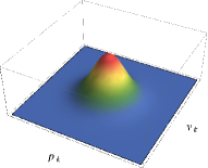
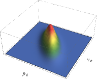
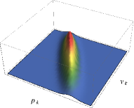
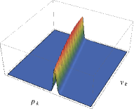
Figure 2: Wigner function of a squeezed quantum state at different times during inflation. Only the two-dimensional function corresponding to the set of variables $\left(v_{\bm{k}}^{\rm R},p_{\bm{k}}^{\rm R}\right)$ has been represented, see Eq. (3). The time evolution of $\Re\mathrm{e}\,\Omega_{\bm{k}}$ and $\Im\mathrm{m}\,\Omega_{\bm{k}}$ has been calculated using the Schrödinger equation with the Hamiltonian that can be obtained from the relativistic theory of cosmological perturbations. The left panel corresponds to $r_{\bm{k}}=0.0005$ and the corresponding state is almost a coherent one. Then, from left to right, one has $r_{\bm{k}}=0.48$, $r_{\bm{k}}=0.88$ and, finally, $r_{\bm{k}}=2.31$ for the right panel. The effect of the squeezing and the cigar shape of Eq. (3) are clearly visible.

A convenient tool to study this question is the Wigner function, defined by

$$W\left(v_{\bm{k}}^{\rm R},v_{\bm{k}}^{\rm I},p_{\bm{k}}^{\rm R},p_{\bm{k}}^{\rm I}\right)=\frac{1}{(2\pi)^{2}}\int{\rm d}x{\rm d}y\,\Psi^{*}\left(v_{\bm{k}}^{\rm R}-\frac{x}{2},v_{\bm{k}}^{\rm I}-\frac{y}{2}\right){\rm e}^{-ip_{\bm{k}}^{\rm R}x-ip_{\bm{k}}^{\rm I}y}\,\Psi\left(v_{\bm{k}}^{\rm R}+\frac{x}{2},v_{\bm{k}}^{\rm I}+\frac{y}{2}\right).$$ (6)

It is well known that the Wigner function can be understood as a classical probability distribution function whenever it is positive definite. Then, upon using the quantum state (3), the following explicit form is obtained

$$W\left(v_{\bm{k}}^{\rm R},v_{\bm{k}}^{\rm I},p_{\bm{k}}^{\rm R},p_{\bm{k}}^{\rm I}\right)=\Psi\Psi^{*}\frac{1}{2\pi\Re\mathrm{e}\,\Omega_{\bm{k}}} \exp\left[-\frac{1}{2\Re\mathrm{e}\,\Omega_{\bm{k}}}\left(p_{\bm{k}}^{\rm R}+2\Im\mathrm{m}\,\Omega_{\bm{k}}v_{\bm{k}}^{\rm R}\right)^{2}\right]$$

$$\times\exp\left[-\frac{1}{2\Re\mathrm{e}\,\Omega_{\bm{k}}}\left(p_{\bm{k}}^{\rm I}+2\Im\mathrm{m}\,\Omega_{\bm{k}}v_{\bm{k}}^{\rm I}\right)^{2}\right].$$ (7)

This Wigner function (3) is represented in Fig. 2 at different times or, equivalently, at different values of $r_{\bm{k}}$ ($r_{\bm{k}}=0.0005$, $0.48$, $0.88$ and $2.31$). The effect of strong squeezing is clearly visible. Initially, in the sub-Hubble regime, $r_{\bm{k}}$ is small and the Wigner function is peaked over of small region in phase space. In this regime, $W$ is just the Wigner function of a coherent state since we chose to start from the ground state of a harmonic oscillator. Coherent states are considered as the “most classical” states precisely for this reason: if one is given, say, the value of $v_{\bm{k}}^{\rm R}$, then one obtains a value for the momentum, $p_{\bm{k}}^{\rm R}$, which is very close to the one one would have inferred in the classical case. This is of course due to the fact that the Wigner function follows the classical trajectory and has minimal spread around it in all phase space directions.

As inflation proceeds, the situation described before changes. The modes become super Hubble and $r_{\bm{k}}(\eta)$ increases. As a consequence, the Wigner function spreads and acquires a cigar shape typical of squeezed states [27]. Therefore, if one is now given $p_{\bm{k}}^{\rm R}$ then the value of $v_{\bm{k}}^{\rm R}$ is very uncertain since the Wigner function is spread over a large region in phase space. In this case, cosmological perturbations certainly do not behave classically in the usual sense. Given the previous discussion, it may seem relatively easy to observe genuine quantum effects in the CMB. Unfortunately this is not so, essentially because, in the strong squeezed limit, all quantum predictions can be in fact obtained from averages performed by mean of a classical stochastic process. The point is that, in the limit $r_{\bm{k}}\rightarrow\infty$, all the quantum predictions can be reproduced if one assumes that the system always followed classical laws but had random initial conditions with a given probability density function. This is possible because the Wigner function, despite being delocalized over phase space, remains positive. This property is not general but is a key feature of Gaussian states, hence of squeezed states.

Let us say a few words about the density matrix $\hat{\rho}_{\bm{k}}^{\rm R}$. The density matrix is nothing but the Fourier transform of the Wigner function. Let us denote by $|v_{\bm{k}}^{\rm R}\rangle$ the eigenstates of the operator $\hat{v}_{\bm{k}}^{\rm R}$. Then, we have

$$\left\langle v_{\bm{k}}^{\rm R}{}^{\prime}\left|\hat{\rho}_{\bm{k}}^{\rm R}\right|v_{\bm{k}}^{\rm R}\right\rangle=\int_{-\infty}^{\infty}{\rm d}y\,{\rm e}^{iy(v_{\bm{k}}^{\rm R}{}^{\prime}-v_{\bm{k}}^{\rm R})}W\left(\frac{v_{\bm{k}}^{\rm R}{}^{\prime}+v_{\bm{k}}^{\rm R}}{2},y\right).$$ (8)

Upon using Eq. (3) in the above equation, one obtains the following expression

$$\left\langle v_{\bm{k}}^{\rm R}{}^{\prime}\left|\hat{\rho}_{\bm{k}}^{\rm R}\right|v_{\bm{k}}^{\rm R}\right\rangle = \left(\frac{2\Re\mathrm{e}\,\Omega_{\bm{k}}}{\pi}\right)^{1/2}{\rm e}^{-\Re\mathrm{e}\,\Omega_{\bm{k}}\left[\left(v_{\bm{k}}^{\rm R}{}^{\prime}\right)^{2}+\left(v_{\bm{k}}^{\rm R}\right)^{2}\right]}{\rm e}^{-i\Im\mathrm{m}\,\Omega_{\bm{k}}\left[\left(v_{\bm{k}}^{\rm R}{}^{\prime}\right)^{2}-\left(v_{\bm{k}}^{\rm R}\right)^{2}\right]}\,.$$ (9)

We notice that the off-diagonal terms, $v_{\bm{k}}^{\rm R}{}^{\prime}\neq v_{\bm{k}}^{\rm R}$, oscillate very rapidly in the strong squeezing limit where $\Im\mathrm{m}\,\Omega_{\bm{k}}\rightarrow\infty$. This means that decoherence (defined as the disappearance of those off-diagonal terms) does not occur without taking into account the influence of an environment for the perturbations. Various discussions on what this environment may be can be found in Refs. [35, 36, 37].

We end this section by a brief discussion of how the theory presented above can make astrophysical predictions. The perturbations described by the Mukhanov-Sasaki variable are directly related to CMB fluctuations. As a consequence, in order to calculate the statistical properties of the CMB, it is sufficient to evaluate the power spectrum of the operator $\hat{v}(\eta,{\bm{x}})$ (and the higher order correlation functions if one is interested in non-Gaussianity). It is given by the following expression

$$\left\langle\Psi\left|\hat{v}(\eta,{\bm{x}})\hat{v}(\eta,{\bm{x}}+{\bm{r}})\right|\Psi\right\rangle=\int\prod_{\bm{k}}{\rm d}v_{\bm{k}}^{\rm R}{\rm d}v_{\bm{k}}^{\rm I}\Psi_{\bm{k}}^{*}(v_{\bm{k}}^{\rm R},v_{\bm{k}}^{\rm I})v(\eta,{\bm{x}})v(\eta,{\bm{x}}+{\bm{r}})\Psi_{\bm{k}}(v_{\bm{k}}^{\rm R},v_{\bm{k}}^{\rm I}).$$ (10)

and, upon using the results exposed before, can be expressed as

$$\left\langle\Psi\left|\hat{v}(\eta,{\bm{x}})\hat{v}(\eta,{\bm{x}}+{\bm{r}})\right|\Psi\right\rangle=\int_{0}^{+\infty}\frac{{\rm d}k}{k}\frac{\sin kr}{kr}{\cal P}_{v}(k)\,,$$ (11)

which, in fact, defines the power spectrum ${\cal P}_{v}(k)$ as the square of the Fourier amplitude per logarithmic interval at a given scale, i.e. ${\cal P}_{v}(k)=k^{3}|f_{\bm{k}}|^{2}/(2\pi^{2})$. On large scales, one obtains ${\cal P}_{\zeta}(k)\simeq A_{{}_{\rm S}}k^{n_{{}_{\rm S}}-1}$ where the coefficients $A_{{}_{\rm S}}$ and $n_{{}_{\rm S}}$ (the spectral index) depend on the inflationary model under consideration. For any “good” model of inflation, one has $n_{{}_{\rm S}}\simeq 1$ but $n_{{}_{\rm S}}\neq 1$. This means that inflation does not predict a scale-invariant power spectrum as sometimes said but an almost scale-invariant power spectrum. This difference is not a detail as a scale-invariant power spectrum (or a Harrison-Zeldovitch power spectrum) was considered well before the advent of inflation. In this case, $n_{{}_{\rm S}}=1$ would just be a postdiction. On the contrary, $n_{{}_{\rm S}}\simeq 1$ but $n_{{}_{\rm S}}\neq 1$ is a prediction of inflation. This prediction has not yet be confirmed by the observations but there is good evidence that it is true. For instance, the WMAP data indicate that $1-n_{{}_{\rm S}}=0.018^{+0.019}_{-0.02}$ [20, 21, 22]). In a few months, with the data of the Planck satellite, this prediction will be definitively confirmed or ruled out with certainty (i.e. at the $5\sigma$ confidence level). Of course, the spectral index is not the only quantity of interest and a list and a discussion of all the inflationary predictions can be found in Refs. [13, 14, 15].

4 Conclusions

In this short letter, we have discussed the quantum-mechanical aspect of inflationary fluctuations. In particular, we have argued that cosmological fluctuations are placed in a very peculiar quantum state, namely a strongly squeezed state. In the very same way that the CMB radiation represents the most accurate black body radiation ever produced (recall that, in the laboratory, it is not possible to produced such an accurate black body), the squeezed state of the inflationary perturbations probably represents the strongest squeezed state ever observed in Nature. As a consequence, one could be led to conclude that the quantum properties of the CMB anisotropies are highly non-classical. And, in a sense, they are! But, we have also shown that everything turns out to be equivalent to a classical stochastic process. Therefore, even if the statistical nature of the fluctuations is here to remind us about their quantum origin, all the genuine quantum-mechanical imprints (such as interferences or the off-diagonal terms in the density matrix) are “washed out” by the strong squeezing and by decoherence. This explains why astronomers can forget about the quantum origin of the CMB fluctuations and consider that they are simply described by a Gaussian stochastic process.

There remains, however, an open question, namely the issue of definite outcomes. This issue is of course already present in conventional quantum mechanics (decoherence does not solve the definite outcome problem, see Ref. [54]) but it is clearly more embarrassing in the context of cosmology where no observer was present during inflation [38]. This problem was recently discussed in Ref. [55]. This is usually taken as an indication that the Copenhagen interpretation is not well suited to cosmology and that other theoretical frameworks, such as (for instance) the many worlds interpretation or the collapse theories, should be considered. This also shows that inflation is not only a scenario which allows us to convincingly reproduce various astrophysical observations but is also a playground where very fundamental questions can be discussed and studied. Usually this is considered to be a feature of quantum cosmology only but, in fact, this is also the case for inflation. It is clear that quantum effects in the context of inflation are treated in a perfectly standard way and, moreover, that we have at our disposal detailed observations that directly originate from those quantum effects. For this reason, it does not seem necessary to go as far as quantum cosmology (although it is of course interesting) to discuss very fundamental questions at the crossroads of quantum mechanics and gravity: inflation can do the job!

References

References

- [1] Starobinsky A A 1980 Phys. Lett. B91 99–102
- [2] Guth A H 1981 Phys. Rev. D23 347–356
- [3] Linde A D 1982 Phys. Lett. B108 389–393
- [4] Albrecht A and Steinhardt P J 1982 Phys. Rev. Lett. 48 1220–1223
- [5] Linde A D 1983 Phys. Lett. B129 177–181
- [6] Mukhanov V F and Chibisov G 1981 JETP Lett. 33 532–535
- [7] Mukhanov V F and Chibisov G 1982 Sov. Phys. JETP 56 258–265
- [8] Starobinsky A A 1982 Phys. Lett. B117 175–178
- [9] Guth A H and Pi S Y 1982 Phys. Rev. Lett. 49 1110–1113
- [10] Hawking S 1982 Phys. Lett. B115 295 revised version
- [11] Bardeen J M, Steinhardt P J and Turner M S 1983 Phys. Rev. D28 679
- [12] Mukhanov V F, Feldman H and Brandenberger R H 1992 Phys.Rept. 215 203–333
- [13] Martin J 2004 Braz. J. Phys. 34 1307–1321 (Preprint %****␣jerome_martin.bbl␣Line␣50␣****astro-ph/0312492)
- [14] Martin J 2005 Lect. Notes Phys. 669 199–244 (Preprint hep-th/0406011)
- [15] Martin J 2008 Lect. Notes Phys. 738 193–241 (Preprint 0704.3540)
- [16] Linde A D 2008 Lect. Notes Phys. 738 1–54 (Preprint 0705.0164)
- [17] Sriramkumar L 2009 (Preprint 0904.4584)
- [18] Peter P and Uzan J P 2009 Primordial Cosmology Oxford Graduate Texts (Oxford University Press)
- [19] Stewart E D and Lyth D H 1993 Phys.Lett. B302 171–175 (Preprint gr-qc/9302019)
- [20] Larson D, Dunkley J, Hinshaw G, Komatsu E, Nolta M et al. 2011 Astrophys.J.Suppl. 192 16 (Preprint 1001.4635)
- [21] Komatsu E et al. (WMAP Collaboration) 2011 Astrophys.J.Suppl. 192 18 (Preprint 1001.4538)
- [22] Martin J and Ringeval C 2006 JCAP 0608 009 (Preprint astro-ph/0605367)
- [23] Lorenz L, Martin J and Ringeval C 2008 JCAP 0804 001 (Preprint 0709.3758)
- [24] Lorenz L, Martin J and Ringeval C 2008 Phys.Rev. D78 063543 (Preprint 0807.2414)
- [25] Martin J and Ringeval C 2010 Phys.Rev. D82 023511 (Preprint 1004.5525)
- [26] Martin J, Ringeval C and Trotta R 2011 Phys.Rev. D83 063524 (Preprint 1009.4157)
- [27] Grishchuk L and Sidorov Y 1990 Phys.Rev. D42 3413–3421
- [28] Grishchuk L, Haus H and Bergman K 1992 Phys.Rev. D46 1440–1449
- [29] Polarski D and Starobinsky A A 1996 Class.Quant.Grav. 13 377–392 (Preprint gr-qc/9504030)
- [30] Lesgourgues J, Polarski D and Starobinsky A A 1997 Nucl.Phys. B497 479–510 (Preprint gr-qc/9611019)
- [31] Grishchuk L and Martin J 1997 Phys.Rev. D56 1924–1938 (Preprint gr-qc/9702018)
- [32] Kiefer C, Lohmar I, Polarski D and Starobinsky A A 2007 Class.Quant.Grav. 24 1699–1718 (Preprint astro-ph/0610700)
- [33] Kiefer C, Polarski D and Starobinsky A A 1998 Int.J.Mod.Phys. D7 455–462 (Preprint gr-qc/9802003)
- [34] Egusquiza I, Feinstein A, Perez Sebastian M and Valle Basagoiti M 1998 Class.Quant.Grav. 15 1927–1936 (Preprint gr-qc/9709061)
- [35] Anderson P R, Molina-Paris C and Mottola E 2005 Phys.Rev. D72 043515 (Preprint hep-th/0504134)
- [36] Burgess C P, Holman R and Hoover D 2008 Phys.Rev. D77 063534 (Preprint astro-ph/0601646)
- [37] Martineau P 2007 Class.Quant.Grav. 24 5817–5834 (Preprint astro-ph/0601134)
- [38] Sudarsky D 2011 Int.J.Mod.Phys. D20 509–552 (Preprint 0906.0315)
- [39] Lyth D H and Riotto A 1999 Phys.Rept. 314 1–146 (Preprint hep-ph/9807278)
- [40] Starobinsky A A 1986
- [41] Martin J and Musso M 2006 Phys. Rev. D73 043516 (Preprint hep-th/0511214)
- [42] Bardeen J M 1980 Phys.Rev. D22 1882–1905
- [43] Martin J and Schwarz D J 1998 Phys.Rev. D57 3302–3316 (Preprint gr-qc/9704049)
- [44] Kodama H and Sasaki M 1984 Prog.Theor.Phys.Suppl. 78 1–166
- [45] Schwinger J S 1951 Phys.Rev. 82 664–679
- [46] Brezin E and Itzykson C 1970 Phys.Rev. D2 1191–1199
- [47] Moore G T 1970 Journal of Mathematical Physics 11 2679–2691
- [48] Wilson C M, Johansson G, Pourkabirian A, Simoen M, Johansson J R, Duty T, Nori F and Delsing P 2011 Nature 479 376–379 (Preprint 1105.4714)
- [49] Birrell N D and Davies P C W 1982 Quantum Fields In Curved Space (Cambridge Univ. Pr.)
- [50] Vahlbruch H, Mehmet M, Chelkowski S, Hage B, Franzen A, Lastzka N, Goßler S, Danzmann K and Schnabel R 2008 Physical Review Letters 100 033602 (Preprint 0706.1431)
- [51] Kiefer C 2000 Nucl.Phys.Proc.Suppl. 88 255–258 (Preprint astro-ph/0006252)
- [52] Caves C M and Schumaker B L 1985 Phys.Rev. A31 3068–3092
- [53] Schumaker B L and Caves C M 1985 Phys.Rev. A31 3093–3111
- [54] Colanero K 2012 ArXiv e-prints (Preprint 1208.0904)
- [55] Martin J, Vennin V and Peter P 2012 (Preprint 1207.2086)