Inflationary Perturbations: the Cosmological Schwinger Effect

Abstract

This pedagogical review aims at presenting the fundamental aspects of the theory of inflationary cosmological perturbations of quantum-mechanical origin. The analogy with the well-known Schwinger effect is discussed in detail and a systematic comparison of the two physical phenomena is carried out. In particular, it is demonstrated that the two underlying formalisms differ only up to an irrelevant canonical transformation. Hence, the basic physical mechanisms at play are similar in both cases and can be reduced to the quantization of a parametric oscillator leading to particle creation due to the interaction with a classical source: pair production in vacuum is therefore equivalent to the appearance of a growing mode for the cosmological fluctuations. The only difference lies in the nature of the source: an electric field in the case of the Schwinger effect and the gravitational field in the case of inflationary perturbations. Although, in the laboratory, it is notoriously difficult to produce an electric field such that pairs extracted from the vacuum can be detected, the gravitational field in the early universe can be strong enough to lead to observable effects that ultimately reveal themselves as temperature fluctuations in the Cosmic Microwave Background. Finally, the question of how quantum cosmological perturbations can be considered as classical is discussed at the end of the article.

1 Introduction

The scenario of inflation was invented in order to solve puzzling issues associated with the standard hot Big Bang theory guth ; inflation . Soon after its advent, it was realized that this scenario also contains a remarkable extra bonus: it gives a well-motivated mechanism for structure formation that leads to a nearly scale-invariant power spectrum MuChi ; pert , namely exactly what is needed in order to account for various astrophysical observations in a satisfactory way wmap . However, this is not the only aspect that deserves to be stressed. Indeed, even from a fundamental point of view, this mechanism appears quite remarkable in the sense that it combines general relativity with quantum mechanics. The main purpose of this review article is to thoroughly discuss this aspect of the theory of inflationary cosmological perturbations.

This theory is in fact remarkable at two levels. Firstly, because it relies on the phenomenon of particle creation which is a non-trivial effect in quantum field theory. In this sense, it is equivalent to the well-known Schwinger schwinger effect and this analogy will be made explicit in this paper. The basic ingredient is a quantum scalar field $\Phi$ (in practice this is rather a fermionic field $\Psi$ but, for simplicity, we will restrict ourselves to the case of a scalar field) interacting with a classical source, in the case of the Schwinger effect, an electric field $E$. The Schwinger effect has not yet been observed in the laboratory as it is difficult to produce an electric field with the required strength but there are prospects to do so, in particular at DESY with a Free Electron Laser (FEL) in the X-ray band Ring ; AHRSV ; xfel but also at SLAC with the Linac Coherent Light Source (LCLS) linac . Even if there is absolutely no reason to doubt the reality of the Schwinger effect, observing pair creation in the laboratory would clearly be a breakthrough and, in some sense, a verification of the corresponding inflationary mechanism.

Secondly, the theory of cosmological perturbations is also remarkable for the following reason. In cosmology, what plays the role of the constant electric field $E$ [originating from a time-dependent potential vector $A_{\mu}(t)$] is the background gravitational field, i.e. the Friedmann-Lemaître-Robertson-Walker (FLRW) scale factor $a(t)$, and what plays the role of the quantum fermionic field $\Psi(t,\vec{x})$ is the quantum perturbed metric $\delta g_{\mu\nu}(t,\vec{x})$, that is to say the small inhomogeneous fluctuations of the gravitational field itself MFB . In the early Universe, the gravitational field is quite strong, i.e. for instance $H/m_{{}_{\mathrm{Pl}}}\sim 10^{-5}$, where $H$ is the Hubble parameter, and this is why the cosmological version of the Schwinger effect can be efficient. From the previous considerations, it is also clear that, in some sense, the inflationary mechanism relies on quantum gravity which adds another interesting aspect to the problem. Of course, we only deal with linearized quantum gravity and this is why we do not have to face tricky questions associated with finiteness of quantum gravity and/or renormalization. More precisely, in the case of scalar perturbations, $\delta g_{\mu\nu}(t,\vec{x})$ is replaced by the Mukhanov-Sasaki variable $v(t,\vec{x})$ which is a combination of the Bardeen potential (the generalization of the Newtonian potential in general relativity) and of the small fluctuations in the inflaton field. For gravitational waves, the relevant quantity is $h_{ij}(t,\vec{x})$, the transverse and traceless part of the perturbed metric.

Let us notice that the two above-mentioned aspects are features of the theory of cosmological perturbations in general. The inflationary aspect is in fact not necessary in order to have particles creation: only a dynamical background is required. However, a quasi-exponential expansion is mandatory if one wants to obtain a power spectrum which is close to scale invariance as indicated by astrophysical observations.

The fact that the inflationary mechanism for structure formation relies on general relativity and quantum mechanics also raises fundamental interpretational questions. In particular, the question of how classicality emerges is of special relevance in this context GP ; PS . Indeed, the perturbations are of quantum-mechanical origin but no astrophysical observations suggest any typically quantum-mechanical signature. Therefore, it is necessary to understand how the perturbations have become classical (and in which sense). This leads to very deep issues. For instance, if one invokes a mechanism based on the phenomenon of decoherence Zurek , then one has to discuss what plays the role of the environment. This question is clearly non-trivial in the cosmological context. At the end of this review article, we will address these questions using the Wigner function wigner as a tool to understand when a system can be considered as classical.

This paper can be viewed as the third of a series on the inflationary theory, the two first ones being Refs. procbrazil ; procpoland . The topics developed in those last two references will be supposed to be known and we will often refer to them. The present paper is organized as follows. In Sec. 2, we briefly review the Schwinger effect. In particular, we derive the rate of pair production in the Schrödinger functional approach and stress the importance of the Wentzel-Kramers-Brillouin (WKB) approximation as a method to choose a well-defined initial state. In Sec. 3, we quantize a free scalar field in a FLRW Universe and show that the basic physical phenomenon at play is equivalent to that responsible for the Schwinger effect, namely particle creation under the influence of a classical source. In particular, we demonstrate that, up to a canonical transformation, the underlying formalisms are the same. Roughly speaking, in both cases, one has to deal with parametric oscillators. The only difference between the two systems lies in the time dependence of the corresponding effective frequencies. In Sec. 4, we argue that the equations obeyed by the cosmological perturbations (in particular during inflation) are equivalent to the equations of motion of a free scalar field. We emphasize that the relevant observable quantity is the two-point correlation function since it is directly linked to the Cosmic Microwave Background (CMB) temperature fluctuations. Finally, as mentioned above, in Sec. 5, we address the question of the classicality of the cosmological perturbations.

2 The Schwinger Effect

2.1 General Formalism

The action of a complex (charged) scalar field interacting with an electromagnetic field is given by

$$S=-\int{\rm d}^{4}x\left(\frac{1}{2}\eta^{\alpha\beta}{\cal D}_{\alpha}\Phi{\cal D}_{\beta}\Phi^{*}+\frac{1}{2}m^{2}\Phi\Phi^{*}\right)\,,$$ (1)

where $\eta^{\alpha\beta}$ is the flat (Minkowski) space-time metric with signature $(-,+,+,+)$ and where the covariant derivative can be expressed as

$${\cal D}_{\alpha}\Phi\equiv\partial_{\alpha}\Phi+iqA_{\alpha}\Phi\,,$$ (2)

$q$ being the charge of the field. The quantity $m$ represents the mass of the scalar particle. Assuming the following configuration for the vector potential $A_{\mu}=(0,0,0,-Et)$, where $E$ is the magnitude of the static electric field aligned along the $z$ direction (by convention), one obtains the following equation of motion

$$\partial_{t}^{2}\Phi-\partial^{i}\partial_{i}\Phi+2iqEt\partial_{z}\Phi+q^{2}E^{2}t^{2}\Phi+m^{2}\Phi=0\,.$$ (3)

It turns out to be more convenient to Fourier transform the field since this allows us to study the evolution of the system mode by mode. For this purpose, one decomposes the field according to

$$\Phi(t,\vec{x})=\frac{1}{(2\pi)^{3/2}}\int{\rm d}^{3}\vec{k}\,\Phi_{\vec{k}}(t){\rm e}^{i\vec{k}\cdot\vec{x}}\,.$$ (4)

In the above expression, $\Phi_{\vec{k}}(t)$ is the time-dependent Fourier amplitude of the mode characterized by the wave-vector $\vec{k}$. Inserting the Fourier transform (4) into Eq. (1), the action of the system takes the form

$$S=-\int{\rm d}t\int_{\mathbb{R}^{3}}{\rm d}\vec{k}\left[-\dot{\Phi}_{\vec{k}}\dot{\Phi}_{\vec{k}}^{*}+\left(k^{2}-2qEk_{z}t+q^{2}E^{2}t^{2}+m^{2}\right)\Phi_{\vec{k}}\Phi_{\vec{k}}^{*}\right]\,,$$ (5)

where a dot denotes a derivative with respect to time. The variation of this Lagrangian with respect to $\Phi_{\vec{k}}^{*}$ and $\dot{\Phi}_{\vec{k}}^{*}$ leads to

$$\frac{\delta\bar{\cal L}}{\delta\Phi_{\vec{k}}^{*}}=-\left(k^{2}-2qEk_{z}t+q^{2}E^{2}t^{2}+m^{2}\right)\Phi_{\vec{k}}\,,\quad\frac{\delta\bar{\cal L}}{\delta\dot{\Phi}_{\vec{k}}^{*}}\equiv p_{k}=\dot{\Phi}_{\vec{k}}\,,$$ (6)

where $p_{k}$ is the conjugate momentum of the Fourier component of the field and $\bar{\cal L}$ denotes the Lagrangian density in Fourier space. Using the two above formula, the Euler-Lagrange equation of motion reads

$$\ddot{\Phi}_{\vec{k}}+\omega^{2}(k,t)\Phi_{\vec{k}}=0\,,$$ (7)

where the time dependent frequency $\omega(k,t)$ can be expressed as

$$\omega^{2}(k,t)\equiv k^{2}-2qEk_{z}t+q^{2}E^{2}t^{2}+m^{2}\,.$$ (8)

Eq. (7) is of course similar to the one one would have obtained by directly substituting Eq. (4) into Eq. (3). It is the equation of motion of a parametric oscillator. Let us recall that a parametric oscillator is an harmonic oscillator whose frequency depends on time. A typical example is a pendulum with a varying length.

Let us now pass to the Hamiltonian formalism. The Hamiltonian is obtained from the Lagrangian by a standard Legendre transformation and can be expressed as

$$H=\int_{\mathbb{R}^{3}}{\rm d}\vec{k}\left(p_{k}\dot{\Phi}_{\vec{k}}^{*}+p_{k}^{*}\dot{\Phi}_{\vec{k}}-\bar{\cal L}\right)=\int_{\mathbb{R}^{3}}{\rm d}\vec{k}\left[p_{k}p_{k}^{*}+\omega^{2}\left(k,t\right)\Phi_{\vec{k}}\Phi_{\vec{k}}^{*}\right]\,.$$ (9)

For the following considerations, it turns out to be convenient to also work with real variables instead of the complex $\Phi_{\vec{k}}$. Therefore, we now introduce the definitions

$$\Phi_{\vec{k}}\equiv\frac{1}{\sqrt{2}}\left(\Phi^{{}_{\mathrm{R}}}_{\vec{k}}+i\Phi^{{}_{\mathrm{I}}}_{\vec{k}}\right)\,,\quad p_{\vec{k}}\equiv\frac{1}{\sqrt{2}}\left(p^{{}_{\mathrm{R}}}_{\vec{k}}+ip^{{}_{\mathrm{I}}}_{\vec{k}}\right)\,.$$ (10)

Then, the Hamiltonian can be written as

$$H=\int_{\mathbb{R}^{3}}{\rm d}\vec{k}\left[\frac{1}{2}\left(p^{{}_{\mathrm{R}}}_{\vec{k}}\right)^{2}+\frac{1}{2}\omega^{2}\left(k,t\right)\left(\Phi^{{}_{\mathrm{R}}}_{\vec{k}}\right)^{2}+\frac{1}{2}\left(p^{{}_{\mathrm{I}}}_{\vec{k}}\right)^{2}+\frac{1}{2}\omega^{2}\left(k,t\right)\left(\Phi^{{}_{\mathrm{I}}}_{\vec{k}}\right)^{2}\right]\,.$$ (11)

One recognizes the Hamiltonian of a collection of parametric oscillators with a time-dependent frequency given by Eq. (8). Again, one can check that the Hamilton equations deduced from Eqs. (9) and (11) lead to an equation of motion similar to the one already derived before, namely Eq. (7).

2.2 Quantization

Our next step is to describe the quantization of the system. More precisely, the complex scalar field is quantized while the gauge field remains classical. Therefore, we have to deal with the interaction of a quantum field with a classical source. Quantization is achieved by requiring the following commutation relations (a hat symbol is put on letters denoting operators)

$$\left[\hat{\Phi}^{{}_{\mathrm{R}}}_{\vec{k}},\hat{p}^{{}_{\mathrm{R}}}_{\vec{p}}\right]=i\delta^{(3)}\left(\vec{k}-\vec{p}\right)\,,\quad\left[\hat{\Phi}^{{}_{\mathrm{I}}}_{\vec{k}},\hat{p}^{{}_{\mathrm{I}}}_{\vec{p}}\right]=i\delta^{(3)}\left(\vec{k}-\vec{p}\right)\,.$$ (12)

We choose to work in the Schrödinger picture where the states are time-dependent and the operators constant. The above commutation relations admit the following representation

$$\hat{\Phi}^{{}_{\mathrm{R}}}_{\vec{k}}\Psi=\Phi^{{}_{\mathrm{R}}}_{\vec{k}}\Psi\,,\quad\hat{p}^{{}_{\mathrm{R}}}_{\vec{k}}\Psi=-i\frac{\partial\Psi}{\partial\Phi^{{}_{\mathrm{R}}}_{\vec{k}}}\,.$$ (13)

The state of the system is described by a functional of the scalar field, $\Psi[\Phi(t,\vec{x})]$ (in the present context, $\Psi$ is the field functional and has clearly nothing to do with the fermionic field mentioned before), which can also be viewed as a function of an infinite number of variables, namely the values of $\Phi$ at each point in space. Alternatively, one can also consider this functional as a function of the infinite number of Fourier components of the field and write

$$\Psi=\prod_{\vec{k}}^{n}\Psi_{\vec{k}}\left(\Phi^{{}_{\mathrm{R}}}_{\vec{k}},\Phi^{{}_{\mathrm{I}}}_{\vec{k}}\right)=\prod_{\vec{k}}^{n}\Psi_{\vec{k}}^{{}_{\mathrm{R}}}\left(\Phi^{{}_{\mathrm{R}}}_{\vec{k}}\right)\Psi_{\vec{k}}^{{}_{\mathrm{I}}}\left(\Phi^{{}_{\mathrm{I}}}_{\vec{k}}\right)\,.$$ (14)

In the above equation, $n$ represents the number of modes that, in the intermediate calculations, it is useful to keep finite (for instance, if we imagine that the field lives in a finite box). However, at the end, we will always consider the continuous case and take the limit $n\rightarrow+\infty$.

In the framework described before, the Schrödinger equation is a functional differential equation. However, the Hamiltonian takes the form of an infinite sum over $\vec{k}$, see for instance Eqs. (9) and (11), without any interaction between different modes. As a consequence, each mode evolves independently and the corresponding Hamiltonian is represented by an ordinary differential operator. Explicitly, one has

$$H_{\vec{k}}\Psi = \left(H_{\vec{k}}^{{}_{\mathrm{R}}}+H_{\vec{k}}^{{}_{\mathrm{I}}}\right)\Psi=-\frac{1}{2}\frac{\partial^{2}\Psi}{\partial\left(\Phi^{{}_{\mathrm{R}}}_{\vec{k}}\right)^{2}}+\frac{1}{2}\omega^{2}(k,t)\left(\Phi^{{}_{\mathrm{R}}}_{\vec{k}}\right)^{2}\Psi-\frac{1}{2}\frac{\partial^{2}\Psi}{\partial\left(\Phi^{{}_{\mathrm{I}}}_{\vec{k}}\right)^{2}}$$ (15)

$$+\frac{1}{2}\omega^{2}(k,t)\left(\Phi^{{}_{\mathrm{I}}}_{\vec{k}}\right)^{2}\Psi\,,$$

where the frequency $\omega$ has been given by Eq. (8).

Let us now consider the ground state of the system described before. We will discuss the choice of the initial conditions and the meaning of the vacuum state in the following but, as is well-known, it is given by a Gaussian state

$$\Psi_{\vec{k}}^{{}_{\mathrm{R}}}\left(t,\Phi^{{}_{\mathrm{R}}}_{\vec{k}}\right)=N_{\vec{k}}\left(t\right){\rm e}^{-\Omega_{\vec{k}}\left(t\right)\left(\Phi^{{}_{\mathrm{R}}}_{\vec{k}}\right)^{2}}\,,\quad\Psi_{\vec{k}}^{{}_{\mathrm{I}}}\left(t,\Phi^{{}_{\mathrm{I}}}_{\vec{k}}\right)=N_{\vec{k}}\left(t\right){\rm e}^{-\Omega_{\vec{k}}\left(t\right)\left(\Phi^{{}_{\mathrm{I}}}_{\vec{k}}\right)^{2}}\,,$$ (16)

where $N_{\vec{k}}(t)$ and $\Omega_{\vec{k}}(t)$ are functions that can be determined using the Schrödinger equation $i\partial_{t}\Psi=H_{\vec{k}}\Psi$. This leads to

$$i\frac{\dot{N}_{\vec{k}}}{N_{\vec{k}}}=\Omega_{\vec{k}}\,,\quad\dot{\Omega}_{\vec{k}}=-2i\Omega_{\vec{k}}^{2}+\frac{i}{2}\omega^{2}\left(k,t\right)\,.$$ (17)

The equation for the complex quantity $\Omega_{\vec{k}}$ is a non-linear Ricatti equation. When a particular solution is known, the general solution can be found by means of two successive quadratures Ince . But this non-linear first order differential equation can also be transformed into a linear second order differential equation. It turns out that this last one is exactly the equation for the Fourier mode function, Eq. (7). Therefore, the solutions to Eqs. (17) read

$$N_{\vec{k}}=\left(\frac{2\Re\Omega_{\vec{k}}}{\pi}\right)^{1/4}\,,\quad\Omega_{\vec{k}}=-\frac{i}{2}\frac{\dot{f}_{\vec{k}}}{f_{\vec{k}}}\,,$$ (18)

where $f_{\vec{k}}$ obeys the equation $\ddot{f}_{\vec{k}}+\omega^{2}(k,t)f_{\vec{k}}=0$, that is to say, as already mentioned, the same equation as the Fourier component of the field, namely Eq. (7). The quantity $N_{\vec{k}}$ is obtained by normalizing the wave-function. One can check that this leads to an equation consistent with the first formula in Eqs. (17). Therefore, one obtains that the ground quantum state of the field is given by

$$\Psi=\prod_{\vec{k}}^{n}\left(\frac{2\Re\Omega_{\vec{k}}}{\pi}\right)^{1/2}{\rm e}^{-\Omega_{\vec{k}}\left(t\right)\left[\left(\Phi^{{}_{\mathrm{R}}}_{\vec{k}}\right)^{2}+\left(\Phi^{{}_{\mathrm{I}}}_{\vec{k}}\right)^{2}\right]}\,.$$ (19)

Once a particular solution for the mode function has been singled out, the functions $N_{\vec{k}}$ and $\Omega_{\vec{k}}$, and hence the wave-function of the field, are completely specified.

One can now use the above-mentioned state in order to calculate the amplitude associated with the transition between two states $\Psi_{1}$ and $\Psi_{2}$. It is defined by

$$\left\langle\Psi_{1}|\Psi_{2}\right\rangle = \int\prod_{\vec{k}}^{n}{\rm d}\Phi^{{}_{\mathrm{R}}}_{\vec{k}}{\rm d}\Phi^{{}_{\mathrm{I}}}_{\vec{k}}\left(\frac{2\Re\Omega_{1,\vec{k}}}{\pi}\right)^{1/2}\left(\frac{2\Re\Omega_{2,\vec{k}}}{\pi}\right)^{1/2}{\rm e}^{-\sum_{\vec{p}}^{n}\left(\Omega_{1,\vec{p}}^{*}+\Omega_{2,\vec{p}}\right)\left(\Phi^{{}_{\mathrm{R}}}_{\vec{p}}\right)^{2}}$$ (20)

$$\times{\rm e}^{-\sum_{\vec{p}}^{n}\left(\Omega_{1,\vec{p}}^{*}+\Omega_{2,\vec{p}}\right)\left(\Phi^{{}_{\mathrm{I}}}_{\vec{p}}\right)^{2}}\,,$$

from which, after having performed the Gaussian integration, one deduces that

$$\left|\left\langle\Psi_{1}|\Psi_{2}\right\rangle\right|^{2} = \det\left[\frac{4\Re\Omega_{1,\vec{k}}\Re\Omega_{2,\vec{k}}}{\left(\Omega_{1,\vec{k}}^{*}+\Omega_{2,\vec{k}}\right)\left(\Omega_{1,\vec{k}}+\Omega_{2,\vec{k}}^{*}\right)}\right]\,.$$ (21)

At this point, one has to use the specific form of $\Omega_{\vec{k}}$, in particular its expression given by Eq. (18) in terms of the function $f_{\vec{k}}$. One obtains

$$\left|\left\langle\Psi_{1}|\Psi_{2}\right\rangle\right|^{2} = \det\left[\frac{\left(\dot{f}_{1,\vec{k}}f_{1,\vec{k}}^{*}-\dot{f}_{1,\vec{k}}^{*}f_{1,\vec{k}}\right)\left(\dot{f}_{2,\vec{k}}f_{2,\vec{k}}^{*}-\dot{f}_{2,\vec{k}}^{*}f_{2,\vec{k}}\right)}{\left(\dot{f}_{1,\vec{k}}^{*}f_{2,\vec{k}}-\dot{f}_{2,\vec{k}}f_{1,\vec{k}}^{*}\right)\left(\dot{f}_{2,\vec{k}}^{*}f_{1,\vec{k}}-\dot{f}_{1,\vec{k}}f_{2,\vec{k}}^{*}\right)}\right]\,.$$ (22)

In this formula $f_{1,\vec{k}}$ is the mode function for the initial state while $f_{2,\vec{k}}$ is the same quantity but for the final state. As usual, one can always expand $f_{2,\vec{k}}$ over the basis $(f_{1,\vec{k}},f_{1,\vec{k}}^{*})$ and write

$$f_{2,\vec{k}}=\alpha_{\vec{k}}f_{1,\vec{k}}+\beta_{\vec{k}}f_{1,\vec{k}}^{*}\,.$$ (23)

Then, using the fact that the Wronskian $\dot{f}_{1,\vec{k}}f_{1,\vec{k}}^{*}-\dot{f}_{1,\vec{k}}^{*}f_{1,\vec{k}}$ is a conserved quantity (as can be easily checked by differentiating it and using the equation satisfied by $f_{\vec{k}}$), one arrives at Kiefer

$$\left|\left\langle\Psi_{1}|\Psi_{2}\right\rangle\right|^{2} = \det\left(\frac{1}{|\alpha_{\vec{k}}|^{2}}\right)\,.$$ (24)

Therefore, the determination of the transition amplitude amounts to integrating the equation controlling the evolution of the mode function. Once this is done, the coefficient $\alpha_{\vec{k}}$ is known and the quantity $\left|\left\langle\Psi_{1}|\Psi_{2}\right\rangle\right|^{2}$ can be determined. In the next section, we discuss an explicit example.

2.3 Particle creation

We now use the formalism developed above in order to study the creation of quantum scalar particles due to interaction with a classical source. This is the well-known Schwinger effect schwinger . In the following, we will demonstrate that the inflationary mechanism for cosmological perturbations is exactly similar to the one discussed here, see also Refs. Kiefer ; SP .

In order to determine the coefficient $\alpha_{\vec{k}}$, one can proceed as follows. Let us use the dimensionless variable $\tau\equiv\sqrt{qE}t-k_{z}/\sqrt{qE}$. Then, the equation of motion for the Fourier component of the field, see Eq. (7), takes the form

$$\frac{{\rm d}^{2}\Phi_{\vec{k}}}{{\rm d}\tau^{2}}+\left(\Upsilon+\tau^{2}\right)\Phi_{\vec{k}}=0\,,$$ (25)

with $\Upsilon\equiv(k_{\perp}^{2}+m^{2})/(qE)$. The quantity $k_{\perp}$ is defined by $k_{\perp}^{2}\equiv k^{2}-k_{z}^{2}=k_{x}^{2}+k_{y}^{2}$ (let us recall that we have chosen an electrical field aligned along the $z$-direction). Eq. (25) can be integrated exactly, see Eq. (9.255.2) of Ref. Grad and the solution can be expressed as

$$\Phi_{\vec{k}}\left(\tau\right)=A_{\vec{k}}D_{-(1+i\Upsilon)/2}\left[\left(1+i\right)\tau\right]+B_{\vec{k}}D_{-(1+i\Upsilon)/2}\left[-\left(1+i\right)\tau\right]\,,$$ (26)

where $A_{\vec{k}}$ and $B_{\vec{k}}$ are two constants fixed by the initial conditions and $D_{p}(z)$ is a parabolic cylinder function of order $p$.

Despite the previous change of variable, Eq. (25) has retained the form of an equation for a parametric oscillator but the frequency is now given by

$$\omega(\tau)\equiv\sqrt{\Upsilon+\tau^{2}}\,.$$ (27)

This equation is well-suited to the WKB approximation. This approximation is not only useful to get an approximate form of the solution but can also be used in order to choose initial conditions that are well-motivated. Here, since we do already know the exact solution, it is clearly this last application we shall be concerned with.

By definition, the WKB mode function $(2\omega)^{-1/2}{\rm e}^{\pm i\int\omega{\rm d}\tau}$ obeys the following equation of motion $\ddot{\Phi}_{\vec{k}}+\left(\omega^{2}-Q\right)\Phi_{\vec{k}}=0$, where the quantity $Q$ is defined by

$$Q\equiv\frac{3}{4}\frac{1}{\omega^{2}}\left(\frac{{\rm d}\omega}{{\rm d}\tau}\right)^{2}-\frac{1}{2}\frac{1}{\omega}\frac{{\rm d}^{2}\omega}{{\rm d}\tau^{2}}\,.$$ (28)

Therefore, one sees that the WKB mode function is a good approximation to the actual one as soon as $|Q/w^{2}|\ll 1$. This last condition defines the regime where the WKB approximation is valid. Let us compute this quantity in the case of Eq. (25). Straightforward calculations lead to the following expression

$$\left|\frac{Q}{\omega^{2}}\right|=\frac{1}{\Upsilon^{2}}\frac{1}{2\left(1+\tau^{2}/\Upsilon\right)^{2}}\left|\frac{5\tau^{2}/\Upsilon}{2\left(1+\tau^{2}/\Upsilon\right)}-1\right|\,,$$ (29)

The quantity $|Q/\omega^{2}|$ is represented in Fig. 1. It is clear that, in the limits $\tau/\sqrt{\Upsilon}\rightarrow\pm\infty$, the WKB approximation is valid. This means that there exists a well-defined vacuum state (or adiabatic vacuum) in the “in” region, $|0^{-}\rangle$, and in the “out” region, $|0^{+}\rangle$.

Figure 1: Evolution of the quantity $|Q/\omega^{2}|$ with time $\tau$ in the case of the Schwinger effect. In the limit $\tau/\sqrt{\Upsilon}\rightarrow\pm\infty$, $|Q/\omega^{2}|$ vanishes and the notion of adiabatic vacuum is available.

When the WKB approximation is satisfied, an approximate solution of the mode functions is available and, as already briefly mentioned above, is given by

$$\Phi_{\vec{k}}\left(\tau\right) \simeq \frac{\alpha_{\vec{k}}}{\sqrt{2\omega}}\exp\left[-i\int_{\tau_{\rm ini}}^{\tau}\omega(\theta){\rm d}\theta\right]+\frac{\beta_{\vec{k}}}{\sqrt{2\omega}}\exp\left[+i\int_{\tau_{\rm ini}}^{\tau}\omega(\theta){\rm d}\theta\right]$$ (30)

$$\equiv \alpha_{\vec{k}}\Phi_{\rm{wkb},\vec{k}}\left(\tau\right)+\beta_{\vec{k}}\Phi_{\rm{wkb},\vec{k}}^{*}\left(\tau\right)\,,$$

where $\tau_{\rm ini}<0$ is some arbitrary initial time.

One can now use the WKB approximation in order to choose an initial state in the following way. We require that the system is in the adiabatic vacuum in the “in” region, $|0^{-}\rangle$, that is to say when $\tau/\sqrt{\Upsilon}\rightarrow-\infty$. Technically, this means that one has $\lim_{\tau/\sqrt{\Upsilon}\rightarrow-\infty}\Phi_{\vec{k}}=\Phi_{\rm{wkb},\vec{k}}$ or $\alpha_{\vec{k}}=1$ and $\beta_{\vec{k}}=0$ (hence satisfying $\left|\alpha_{\vec{k}}\right|^{2}-\left|\beta_{\vec{k}}\right|^{2}=1$). This criterion completely specifies the coefficients $A_{\vec{k}}$ and $B_{\vec{k}}$ in Eq. (26) and, as a consequence, also completely determines the coefficients $\alpha_{\vec{k}}$ and $\beta_{\vec{k}}$ in the “out” region (when $\tau/\sqrt{\Upsilon}\rightarrow+\infty$) that are needed in order to compute the transition amplitude. Around $\tau\sim 0$, see Fig. 1, the WKB approximation is violated and we have particle creation. In the “out” region the vacuum is defined by $|0^{+}\rangle$ and, therefore, the number of particles present in this region is measured by evaluating the amplitude $\langle 0^{-}|0^{+}\rangle$.

We now briefly explain how this can be done at the technical level. The phase can be computed exactly and reads

$$\int_{\tau_{\rm ini}}^{\tau}\omega(\theta){\rm d}\theta = \frac{\Upsilon}{2}\Biggl{[}\frac{\tau}{\sqrt{\Upsilon}}\sqrt{1+\frac{\tau^{2}}{\Upsilon}}-\frac{\tau_{\rm ini}}{\sqrt{\Upsilon}}\sqrt{1+\frac{\tau^{2}_{\rm ini}}{\Upsilon}}$$ (31)

$$+\ln\left(\frac{\tau}{\sqrt{\Upsilon}}+\sqrt{1+\frac{\tau^{2}}{\Upsilon}}\right)-\ln\left(\frac{\tau_{\rm ini}}{\sqrt{\Upsilon}}+\sqrt{1+\frac{\tau_{\rm ini}^{2}}{\Upsilon}}\right)\Biggr{]}\,.$$

The arguments of the logarithms are always positive even if $\tau$ is negative (hence the corresponding expression with $\tau_{\rm ini}<0$ is also meaningful). In the limit $\left|\tau\right|\Upsilon^{-1/2}\gg 1$, the phase goes to

$$\int_{\tau_{\rm ini}}^{\tau}\omega(\theta){\rm d}\theta\rightarrow\frac{1}{2}\left(\tau\left|\tau\right|+\left|\tau_{\rm ini}\right|^{2}\right)+\frac{\Upsilon}{2}\left(\frac{|\tau|}{\tau}\ln\left|\tau\right|+\ln\left|\tau_{\rm ini}\right|\right)$$ (32)

and, therefore, the WKB mode function takes the form

$$\Phi_{\rm{wkb},\vec{k}}=\frac{1}{\sqrt{2}}{\rm e}^{-i\left(\tau|\tau|+\tau_{\rm ini}^{2}\right)/2}\left|\tau\right|^{-1/2-i|\tau|\Upsilon/(2\tau)}\left|\tau_{\rm ini}\right|^{-i\Upsilon/2}\,.$$ (33)

Then, in the limit $\tau\rightarrow-\infty$, the exact solution given by Eq. (26) can be expressed as

$$\Phi_{\vec{k}} \simeq A_{\vec{k}}\frac{\sqrt{2\pi}}{\Gamma\left(\frac{1}{2}+\frac{i\Upsilon}{2}\right)}{\rm e}^{-i\pi\left(1-i\Upsilon\right)/4}\left(1-i\right)^{-\left(1-i\Upsilon\right)/2}\sqrt{2}\,{\rm e}^{i\left|\tau_{\rm ini}\right|^{2}/2}\left|\tau_{\rm ini}\right|^{i\Upsilon/2}\Phi_{\rm{wkb},\vec{k}}$$

$$+ \left[A_{\vec{k}}{\rm e}^{i\pi\left(1+i\Upsilon\right)/2}+B_{\vec{k}}\right]\left(1+i\right)^{-\left(1+i\Upsilon\right)/2}\sqrt{2}\,{\rm e}^{-i\left|\tau_{\rm ini}\right|^{2}/2}\left|\tau_{\rm ini}\right|^{-i\Upsilon/2}\Phi_{\rm{wkb},\vec{k}}^{*}\,.$$

Since, as explained above, we choose the initial state such that $\alpha_{\vec{k}}=1$ and $\beta_{\vec{k}}=0$, this amounts to requiring

$$A_{\vec{k}} = \frac{\Gamma\left(\frac{1}{2}+\frac{i\Upsilon}{2}\right)}{\sqrt{2\pi}}{\rm e}^{i\pi\left(1-i\Upsilon\right)/4}\left(1-i\right)^{\left(1-i\Upsilon\right)/2}\frac{1}{\sqrt{2}}{\rm e}^{-i\left|\tau_{\rm ini}\right|^{2}/2}\left|\tau_{\rm ini}\right|^{-i\Upsilon/2}\,,$$ (35)

$$B_{\vec{k}} = -A_{\vec{k}}{\rm e}^{i\pi\left(1+i\Upsilon\right)/2}\,.$$ (36)

Finally, one considers the behavior of the mode function in the limit $\tau\rightarrow+\infty$ and, using again the WKB mode function is this regime, one can find the corresponding coefficients $\alpha_{\vec{k}}$ and $\beta_{\vec{k}}$. One obtains

$$\left|\alpha_{\vec{k}}\right|^{2}=1+{\rm e}^{-\pi\Upsilon}\,,\quad\left|\beta_{\vec{k}}\right|^{2}={\rm e}^{-\pi\Upsilon}\,.$$ (37)

These expressions still satisfy $\left|\alpha_{\vec{k}}\right|^{2}-\left|\beta_{\vec{k}}\right|^{2}=1$ as required.

We have now reached our final goal and can return to the calculation of the determinant in Eq. (24). Using the coefficient $\alpha_{\vec{k}}$ obtained above, one has

$$\left|\left\langle 0^{-}|0^{+}\right\rangle\right|^{2} = \det\left(\frac{1}{1+{\rm e}^{-\pi\Upsilon}}\right)=\exp\left[-{\rm Tr}\ln\left(1+{\rm e}^{-\pi\Upsilon}\right)\right]\,.$$ (38)

The evaluation of the trace is standard and leads to the well-known result first obtained by Schwinger in the early fifties schwinger

$$\left|\left\langle 0^{-}|0^{+}\right\rangle\right|^{2} = \exp\left[-\frac{VT}{(2\pi)^{3}}\sum_{n=1}^{\infty}\frac{(-1)^{n+1}}{n^{2}}\left(qE\right)^{2}{\rm e}^{-n\pi m^{2}/(qE)}\right]\,.$$ (39)

The physical interpretation of this formula is clear. The argument of the exponential gives the number of pairs created in the space-time volume $VT$ due to the interaction of the quantum scalar field with the classical electric field. One can define a critical electric field (we have restored the fundamental constants) by

$$E_{\rm cri}=\frac{m^{2}c^{3}}{q\hbar}\,,$$ (40)

which is such that the number of particles created is significant only if $E\gg E_{\rm cri}$. This condition can be understood by noting that this is just the requirement that the work performed by the force $qE$ over the Compton length $\lambda=\hbar/(mc)$ is larger than the rest energy $2mc^{2}$. In the case of pairs $e^{+}e^{-}$, the critical electric field is given by $E_{\rm cri}\sim 1.3\times 10^{18}\,\mbox{V}\times\mbox{m}^{-1}$. It is also interesting to remark that the dependence of $\left|\left\langle 0^{-}|0^{+}\right\rangle\right|^{2}$ in $E$ is non-perturbative. This is one of the few example in quantum field theory where an exact result can be obtained (of course, this is not “full quantum theory” but rather “potential theory” since the radiative corrections to the Schwinger mechanism are not taken into account).

We will see that the inflationary mechanism of production of cosmological perturbations is similar to the Schwinger mechanism. Therefore, observing this latter effect in the laboratory could be seen as an indication that we are on the right track as far as the inflationary mechanism is concerned. For instance, at DESY, there are plans to construct a Free Electron Laser (FEL) in the X-ray band which would effectively produce a very strong electric field and, hence, to observe the Schwinger mechanism Ring ; AHRSV . Unfortunately, even with a FEL, it is inconceivable to produce a static field with the required strength given present day technology. However, the situation is different for an oscillating electric field IZ (other configurations have been studied in Refs. FGKA ; AFY ; FY ) and, in this case, it seems possible to extract pairs from the vacuum. This would also be a validation of the Schwinger mechanism since only the time-dependence of $\omega(k,t)$ is changed but not the other basic ingredients. It is also interesting to notice that, in the context of the inflationary theory, this case is in fact very similar to the reheating turner ; preheating stage where the effective frequency of the perturbations is alternating due to the oscillations of the inflaton field at the bottom of its potential.

To conclude this section, let us recall that the basic ingredient at play here is particle creation due to the interaction of a quantum field with a classical source. When the WKB approximation is valid, a well-defined notion of vacuum state exists, and when the WKB approximation is violated, particle creation occurs. We will see that, in the case of inflationary cosmological perturbations, exactly the same mechanism is available.

3 Quantization of a Free Scalar Field in Curved Space-time

Before considering inflation itself, let us now discuss the case of a free real scalar field in curved space-time since this is the simplest example which allows us to capture all the essential features of the theory of inflationary cosmological perturbations.

3.1 General Formalism

We consider the question of quantizing a (massless) scalar field in curved space-time. The starting point is the following action

$$S=-\int{\rm d}^{4}x\sqrt{-g}g^{\mu\nu}\frac{1}{2}\partial_{\mu}\Phi\partial_{\nu}\Phi\,,$$ (41)

which, in a flat FLRW Universe whose metric is given by ${\rm d}s^{2}=a^{2}(\eta)(-{\rm d}\eta^{2}+\delta_{ij}{\rm d}x^{i}{\rm d}x^{j})$, $\eta$ being the conformal time, reads

$$S=\frac{1}{2}\int{\rm d}^{4}xa^{2}(\eta)\left(\Phi^{\prime 2}-\delta^{ij}\partial_{i}\Phi\partial_{j}\Phi\right)\,.$$ (42)

It follows immediately that the conjugate momentum to the scalar field can be expressed as

$$\Pi(\eta,\vec{x})=a^{2}\Phi^{\prime}(\eta,\vec{x})\,,$$ (43)

where a prime denotes a derivative with respect to conformal time. As before, it is convenient to Fourier expand the field $\Phi(\eta,\vec{x})$ over the basis of plane waves (therefore, we make explicit use of the fact that the space-like hyper-surfaces are flat). This gives

$$\Phi(\eta,\vec{x})=\frac{1}{a(\eta)}\frac{1}{(2\pi)^{3/2}}\int{\rm d}\vec{k}\mu_{\vec{k}}(\eta){\rm e}^{i\vec{k}\cdot\vec{x}}\,.$$ (44)

We have chosen to re-scale the Fourier component $\mu_{\vec{k}}$ with a factor $1/a(\eta)$ for future convenience. Since the scalar field is real, one has $\mu_{\vec{k}}^{*}=\mu_{-\vec{k}}$. The next step consists in inserting the expression of $\Phi(\eta,\vec{x})$ into the action (42). This leads to

$$S = \frac{1}{2}\int{\rm d}\eta\int_{\mathbb{R}^{3+}}{\rm d}^{3}\vec{k}\biggl{[}\mu_{\vec{k}}^{\prime}{}^{*}\mu_{\vec{k}}^{\prime}+\mu_{\vec{k}}^{\prime}\mu_{\vec{k}}^{\prime}{}^{*}-2\frac{a^{\prime}}{a}\left(\mu_{\vec{k}}^{\prime}\mu_{\vec{k}}^{*}+\mu_{\vec{k}}^{\prime}{}^{*}\mu_{\vec{k}}\right)$$ (45)

$$+\biggl{(}\frac{a^{\prime}{}^{2}}{a^{2}}-k^{2}\biggr{)}\left(\mu_{\vec{k}}\mu_{\vec{k}}^{*}+\mu_{\vec{k}}^{*}\mu_{\vec{k}}\right)\biggr{]}\,.$$

Notice that the integral over the wave-numbers is calculated over half the space in order to sum over independent variables only cohen . This formula is similar to Eq. (5) for the case of the Schwinger effect (of course, in this last case, we do not have $\Phi_{\vec{k}}=\Phi_{-\vec{k}}^{*}$ since the field is charged and, hence, the integral is performed over all the momentum space).

Equipped with the Lagrangian in the momentum space (which, in the following, as it was the case in the previous Section, we denote by $\bar{\cal L}$), one can check that it leads to the correct equation of motion. Since we have $\delta\bar{\cal L}/\delta\mu_{\vec{k}}^{*}=1/2[-2{\cal H}\mu_{\vec{k}}^{\prime}{}+2({\cal H}^{2}-k^{2})\mu_{\vec{k}}^{\prime}{}]$, the Euler-Lagrange equation ${\rm d}[\delta\bar{\cal L}/\delta\mu_{\vec{k}}^{\prime}{}^{*}]/{\rm d}\eta-\delta\bar{\cal L}/\delta\mu_{\vec{k}}^{*}=0$ reproduces the correct equation of motion for the variable $\mu_{\vec{k}}$, namely

$$\frac{{\rm d}^{2}\mu_{\vec{k}}}{{\rm d}\eta^{2}}+\omega^{2}(k,\eta)\mu_{\vec{k}}=0\,,$$ (46)

that is to say, again, the equation of a parametric oscillator, as in Eq. (7), but with a frequency now given by

$$\omega^{2}(k,\eta)=k^{2}-\frac{a^{\prime\prime}}{a}\,.$$ (47)

This last formula should be compared with Eq. (8). In the case of the Schwinger effect, the frequency was time-dependent because of the interaction of the scalar field with the time-dependent potential vector. Here, the frequency is time-dependent because the scalar field lives in a time-dependent background, or, in some sense, because the scalar field interacts with the classical gravitational background. Therefore, we already see at this stage that we can have particle creation due to the interaction with a classical gravitational field (instead of a classical electric field in the previous Section). Of course, the two cases are not exactly similar in the sense that the time dependence of $\omega^{2}$ is different. Indeed, in the Schwinger case, $\omega^{2}(k,t)$ typically contains terms proportional to $t$ and $t^{2}$, see Eq. (8), while, in the inflationary case, the term $a^{\prime\prime}/a$ is typically proportional to $1/\eta^{2}$. As a consequence, the solution to the mode equation and the particle creation rate will be different even if, again, the basic mechanism at play is exactly the same in both situations.

The mode amplitude $\mu_{\vec{k}}$ is complex but one can also work with real variables $\mu^{{}_{\mathrm{R}}}_{\vec{k}}$ and $\mu^{{}_{\mathrm{I}}}_{\vec{k}}$, as was done previously in Eq. (10), defined such that

$$\mu_{\vec{k}}\equiv\frac{1}{\sqrt{2}}\left(\mu^{{}_{\mathrm{R}}}_{\vec{k}}+i\mu^{{}_{\mathrm{I}}}_{\vec{k}}\right)\,.$$ (48)

In terms of these variables, the relation $\mu_{\vec{k}}^{*}=\mu_{-\vec{k}}$ reads $\mu^{{}_{\mathrm{R}}}_{\vec{k}}=\mu^{{}_{\mathrm{R}}}_{-\vec{k}}$ and $\mu^{{}_{\mathrm{I}}}_{\vec{k}}=-\mu^{{}_{\mathrm{I}}}_{-\vec{k}}$. Then, the action (or Lagrangian) of the system takes the form

$$S = \frac{1}{2}\int{\rm d}\eta\int_{\mathbb{R}^{3+}}{\rm d}^{3}\vec{k}\biggl{\{}\left(\mu^{{}_{\mathrm{R}}}_{\vec{k}}{}^{\prime}\right)^{2}+\left(\mu^{{}_{\mathrm{I}}}_{\vec{k}}{}^{\prime}\right)^{2}-2\frac{a^{\prime}}{a}\left(\mu^{{}_{\mathrm{R}}}_{\vec{k}}\mu^{{}_{\mathrm{R}}}_{\vec{k}}{}^{\prime}+\mu^{{}_{\mathrm{I}}}_{\vec{k}}\mu^{{}_{\mathrm{I}}}_{\vec{k}}{}^{\prime}\right)$$ (49)

$$+\biggl{(}\frac{a^{\prime}{}^{2}}{a^{2}}-k^{2}\biggr{)}\left[\left(\mu^{{}_{\mathrm{R}}}_{\vec{k}}\right)^{2}+\left(\mu^{{}_{\mathrm{I}}}_{\vec{k}}\right)^{2}\right]\biggr{\}}\,.$$

One can check that it also leads to the correct equations of motion for the two real variables $\mu^{{}_{\mathrm{R}}}_{\vec{k}}$ and $\mu^{{}_{\mathrm{I}}}_{\vec{k}}$.

We can now pass to the Hamiltonian formalism. The conjugate momentum to $\mu_{\vec{k}}$ is defined by the formula

$$p_{\vec{k}}\equiv\frac{\delta\bar{{\cal L}}}{\delta\mu_{\vec{k}}^{\prime}{}^{*}}=\mu_{\vec{k}}^{\prime}-\frac{a^{\prime}}{a}\mu_{\vec{k}}\,.$$ (50)

One can check that the definitions of the conjugate momenta in the real and Fourier spaces are consistent in the sense that they are related by the (expected) expression

$$\Pi(\eta,\vec{x})=\frac{a(\eta)}{(2\pi)^{3/2}}\int{\rm d}{\vec{k}}\,p_{\vec{k}}{\rm e}^{i{\vec{k}}\cdot{\vec{x}}}\,.$$ (51)

We see that the definition of the conjugate momentum $p_{\vec{k}}$ as the derivative of the Lagrangian in Fourier space with respect to $\mu_{\vec{k}}^{\prime}{}^{*}$ and not to $\mu_{\vec{k}}^{\prime}$ is consistent with the expression of the momentum in real space. Otherwise the momentum $\Pi(\eta,\vec{x})$ in real space would have been expressed in terms of $p_{\vec{k}}^{*}$ instead of $p_{\vec{k}}$. Moreover, one can also check that

$$p^{{}_{\mathrm{R}}}_{\vec{k}}\equiv\frac{\delta\bar{{\cal L}}}{\delta\mu^{{}_{\mathrm{R}}}_{\vec{k}}{}^{\prime}}=\mu^{{}_{\mathrm{R}}}_{\vec{k}}{}^{\prime}-\frac{a^{\prime}}{a}\mu^{{}_{\mathrm{R}}}_{\vec{k}}\,,\quad p^{{}_{\mathrm{I}}}_{\vec{k}}\equiv\frac{\delta\bar{{\cal L}}}{\delta\mu^{{}_{\mathrm{I}}}_{\vec{k}}{}^{\prime}}=\mu^{{}_{\mathrm{I}}}_{\vec{k}}{}^{\prime}-\frac{a^{\prime}}{a}\mu^{{}_{\mathrm{I}}}_{\vec{k}}\,,$$ (52)

and, clearly, we have

$$p_{\vec{k}}\equiv\frac{1}{\sqrt{2}}\left(p^{{}_{\mathrm{R}}}_{\vec{k}}+ip^{{}_{\mathrm{I}}}_{\vec{k}}\right)\,,$$ (53)

as expected.

We are now in a position where we can compute explicitly the Hamiltonian in the momentum space. The Hamiltonian density, $\bar{\cal H}$, is defined in terms of the Hamiltonian $H$ of the system through the relation

$$H=\int_{\mathbb{R}^{3+}}{\rm d}^{3}\vec{k}\bar{\cal H}=\int_{\mathbb{R}^{3+}}{\rm d}^{3}\vec{k}\left(p_{\vec{k}}\mu_{\vec{k}}^{\prime}{}^{*}+p_{\vec{k}}^{*}\mu_{\vec{k}}^{\prime}-\bar{\cal L}\right)\,,$$ (54)

and we obtain

$$\bar{\cal H}=p_{\vec{k}}p_{\vec{k}}^{*}+k^{2}\mu_{\vec{k}}\mu_{\vec{k}}^{*}+\frac{a^{\prime}}{a}\left(p_{\vec{k}}\mu_{\vec{k}}^{*}+p_{\vec{k}}^{*}\mu_{\vec{k}}\right)\,.$$ (55)

Let us make some comments on this expression. If the background gravitational field is not time-dependent, that is to say if the scalar field lives in Minkowski space-time where $a^{\prime}=0$, then the above Hamiltonian reduces to a free Hamiltonian : there is simply no classical “pump field”. From the Schwinger effect point of view, this would be similar to a situation where there is no external classical electric field. In these two cases, no particle creation would occur. Moreover, one can also check that the Hamilton equations

$$\frac{{\rm d}\mu_{\vec{k}}^{*}}{{\rm d}\eta}=\frac{\partial\bar{\cal H}}{\partial p_{\vec{k}}}=cp_{\vec{k}}^{*}+\frac{a^{\prime}}{a}\mu_{\vec{k}}^{*}\,,\quad\frac{{\rm d}p_{\vec{k}}^{*}}{{\rm d}\eta}=-\frac{\partial\bar{\cal H}}{\partial\mu_{\vec{k}}}=-\frac{a^{\prime}}{a}p_{\vec{k}}^{*}-\frac{k^{2}}{c}\mu_{\vec{k}}^{*}\,,$$ (56)

lead to the correct equation of motion given by Eq. (46). Finally, in terms of the real variables, the Hamiltonian density reads

$$\bar{\cal H}=\frac{1}{2}\left[\left(p^{{}_{\mathrm{R}}}_{\vec{k}}\right)^{2}+2\frac{a^{\prime}}{a}\mu^{{}_{\mathrm{R}}}_{\vec{k}}p^{{}_{\mathrm{R}}}_{\vec{k}}+k^{2}\left(\mu^{{}_{\mathrm{R}}}_{\vec{k}}\right)^{2}\right]+\frac{1}{2}\left[\left(p^{{}_{\mathrm{I}}}_{\vec{k}}\right)^{2}+2\frac{a^{\prime}}{a}\mu^{{}_{\mathrm{I}}}_{\vec{k}}p^{{}_{\mathrm{I}}}_{\vec{k}}+k^{2}\left(\mu^{{}_{\mathrm{I}}}_{\vec{k}}\right)^{2}\right]\,.$$ (57)

We notice that $\bar{\cal H}$ is simply the sum of two identical Hamiltonians for parametric oscillator, one for $\mu^{{}_{\mathrm{R}}}_{\vec{k}}$ and the other for $\mu^{{}_{\mathrm{I}}}_{\vec{k}}$.

The expressions (55) and (57) should be compared to Eqs. (9) and (11). We see that, although similar, the formulae are not identical. However, as we are now going to show, this difference is only apparent. Indeed, let us now restart from the Lagrangian given by Eq. (49). One can always add a total derivative without modifying the underlying theory. If one adds the following term

$$\frac{1}{2}\frac{{\rm d}}{{\rm d}\eta}\left[\frac{a^{\prime}}{a}\left(\mu^{{}_{\mathrm{R}}}_{\vec{k}}\right)^{2}+\frac{a^{\prime}}{a}\left(\mu^{{}_{\mathrm{I}}}_{\vec{k}}\right)^{2}\right]\,,$$ (58)

then the Lagrangian takes the form

$$S = \frac{1}{2}\int{\rm d}\eta\int_{\mathbb{R}^{3+}}{\rm d}^{3}\vec{k}\biggl{\{}\left(\mu^{{}_{\mathrm{R}}}_{\vec{k}}{}^{\prime}\right)^{2}+\left(\mu^{{}_{\mathrm{I}}}_{\vec{k}}{}^{\prime}\right)^{2}-\omega^{2}\left(k,\eta\right)\left[\left(\mu^{{}_{\mathrm{R}}}_{\vec{k}}\right)^{2}+\left(\mu^{{}_{\mathrm{I}}}_{\vec{k}}\right)^{2}\right]\biggr{\}}\,,$$ (59)

where $\omega^{2}(k,\eta)=k^{2}-a^{\prime\prime}/a$. In this case, the conjugate momenta are simply given by $p^{{}_{\mathrm{R}}}_{\vec{k}}=\mu^{{}_{\mathrm{R}}}_{\vec{k}}{}^{\prime}$ and $p^{{}_{\mathrm{I}}}_{\vec{k}}=\mu^{{}_{\mathrm{I}}}_{\vec{k}}{}^{\prime}$. As a consequence, the Hamiltonian now reads

$$H = \int_{\mathbb{R}^{3+}}{\rm d}^{3}\vec{k}\left\{\frac{1}{2}\left(\hat{p}^{{}_{\mathrm{R}}}_{\vec{k}}\right)^{2}+\frac{1}{2}\left(\hat{p}^{{}_{\mathrm{I}}}_{\vec{k}}\right)^{2}+\frac{1}{2}\omega^{2}\left(k,\eta\right)\left[\left(\hat{\mu}^{{}_{\mathrm{R}}}_{\vec{k}}\right)^{2}+\left(\hat{\mu}^{{}_{\mathrm{I}}}_{\vec{k}}\right)^{2}\right]\right\}\,.$$ (60)

This time, the Hamiltonian is exactly similar to the Schwinger Hamiltonian given by Eq. (11). This is another manifestation of the fact that, except for the exact time dependence of the effective frequency, the physical phenomenon, namely particle creation under the influence of an external classical field, is the same in both cases.

Let us now investigate in more detail the relation between the Hamiltonian given by Eq. (57) and the one of Eq. (60). We have just seen that the two corresponding theories differ by a total derivative and, hence, are physically equivalent. Another way to discuss the same property is through a canonical transformation. For this purpose, let us consider the following Hamiltonian

$$H_{1}\left(p_{1},q_{1}\right)=\frac{1}{2}p_{1}^{2}+\frac{a^{\prime}}{a}p_{1}q_{1}+\frac{1}{2}k^{2}q_{1}^{2}\,,$$ (61)

where $a(\eta)$ is an arbitrary function of the time. Clearly, $H_{1}$ plays the role of the Hamiltonian in Eq. (57) and $a(\eta)$ is the scale factor. Then, let us consider a canonical transformation of type II goldstein such that $(q_{1},p_{1})\rightarrow(q_{2},p_{2})$, the generating function of which is given by (a similar transformation has also been studied in Refs. CR ; PPP )

$$G_{2}\left(q_{1},p_{2},\eta\right)=q_{1}p_{2}-\frac{1}{2}\frac{a^{\prime}}{a}q_{1}^{2}\,.$$ (62)

From this function, it is easy to establish the relation between the “old” variables and the “new” ones. One obtains

$$p_{1}=\frac{\partial G_{2}}{\partial q_{1}}=p_{2}-\frac{a^{\prime}}{a}q_{1}\,,\quad q_{2}=\frac{\partial G_{2}}{\partial p_{2}}=q_{1}\,.$$ (63)

In particular, the first relation reproduces Eq. (50) with the correct sign. Finally, the “new” Hamiltonian is given by

$$H_{2}\left(p_{2},q_{2}\right)=H_{1}+\frac{\partial G_{2}}{\partial\eta}=\frac{1}{2}p_{2}^{2}+\frac{1}{2}\left(k^{2}-\frac{a^{\prime\prime}}{a}\right)q_{2}^{2}\,.$$ (64)

Clearly this Hamiltonian is similar to the Hamiltonian of Eq. (60).

Therefore, the two versions of the theory, the one given by the Hamiltonian (57), which is what we naturally obtain in the case of cosmological perturbations (see Sec. 4), and the one which leads to the Hamiltonian (60) “à la Schwinger” are simply connected by a canonical transformation and, thus, are physically identical. In the following, we will see that this is also the case at the quantum level.

3.2 Quantization and the squeezed states formalism

So far, the discussion has been purely classical. We now study the quantization of the system starting with the Heisenberg picture. The quantization in the functional picture that we used for the Schwinger effect will be investigated in the next sub-Section. At the quantum level, $\mu_{\vec{k}}$ and $p_{\vec{k}}$ become operators satisfying the commutation relation

$$\left[\hat{\mu}_{\vec{k}},\hat{p}_{\vec{p}}^{\dagger}\right]=i\delta^{(3)}\left(\vec{k}-\vec{p}\right)\,.$$ (65)

Clearly, factor ordering is now important. The quantum Hamiltonian is obtained from the classical one by properly symmetrizing the expression (55). This leads to

$$\hat{H}=\int_{\mathbb{R}^{3+}}{\rm d}^{3}\vec{k}\left[\hat{p}_{\vec{k}}\hat{p}_{\vec{k}}^{\dagger}+k^{2}\hat{\mu}_{\vec{k}}\hat{\mu}_{\vec{k}}^{\dagger}+\frac{a^{\prime}}{2a}\left(\hat{p}_{\vec{k}}\hat{\mu}_{\vec{k}}^{\dagger}+\hat{\mu}_{\vec{k}}^{\dagger}\hat{p}_{\vec{k}}+\hat{p}_{\vec{k}}^{\dagger}\hat{\mu}_{\vec{k}}+\hat{\mu}_{\vec{k}}\hat{p}_{\vec{k}}^{\dagger}\right)\right]\,.$$ (66)

In addition, this guarantees the hermiticity of the Hamiltonian. The next step consists in introducing the normal variable $\hat{c}_{\vec{k}}$ cohen (which becomes the annihilation operator, $\hat{c}_{\vec{k}}^{\dagger}$ becoming the creation operator) defined by

$$\hat{c}_{\vec{k}}(\eta)\equiv\sqrt{\frac{k}{2}}\hat{\mu}_{\vec{k}}+\frac{i}{\sqrt{2k}}\hat{p}_{\vec{k}}\,.$$ (67)

Equivalently, one can also express $\hat{\mu}_{\vec{k}}$ and $\hat{p}_{\vec{k}}$ in terms of the normal variable and its hermitic conjugate. This gives the following two relations

$$\hat{\mu}_{\vec{k}}=\frac{1}{\sqrt{2k}}\left(\hat{c}_{\vec{k}}+\hat{c}_{-\vec{k}}^{\dagger}\right)\,,\quad\hat{p}_{\vec{k}}=-i\sqrt{\frac{k}{2}}\left(\hat{c}_{\vec{k}}-\hat{c}_{-\vec{k}}^{\dagger}\right)\,.$$ (68)

Then, from the commutation relation (65), or equivalently from the relation in real space $[\hat{\Phi}(\eta,\vec{x}),\hat{\Pi}(\eta,\vec{y})]=i\delta^{(3)}(\vec{x}-\vec{y})$, it follows that $[c_{\vec{k}}(\eta),c_{\vec{p}}^{\dagger}(\eta)]=\delta^{(3)}({\vec{k}}-{\vec{p}})$. In terms of the normal variables, the scalar field and its conjugate momentum can be expressed as

$$\hat{\Phi}(\eta,\vec{k}) = \frac{1}{a(\eta)}\frac{1}{(2\pi)^{3/2}}\int\frac{{\rm d}{\vec{k}}}{\sqrt{2k}}\,\left[\hat{c}_{\vec{k}}(\eta){\rm e}^{i{\vec{k}}\cdot{\vec{x}}}+\hat{c}_{\vec{k}}^{\dagger}(\eta){\rm e}^{-i{\vec{k}}\cdot{\vec{x}}}\right]\,,$$ (69)

$$\hat{\Pi}(\eta,\vec{x}) = -\frac{a(\eta)}{(2\pi)^{3/2}}\int{\rm d}{\vec{k}}\,i\sqrt{\frac{k}{2}}\left[\hat{c}_{\vec{k}}(\eta){\rm e}^{i{\vec{k}}\cdot{\vec{x}}}-\hat{c}_{\vec{k}}^{\dagger}(\eta){\rm e}^{-i{\vec{k}}\cdot{\vec{x}}}\right]\,.$$ (70)

Obviously, when $a^{\prime}=0$, we recover the flat space-time limit and so we expect the time dependence of the normal variables to be just $\hat{c}_{\vec{k}}(\eta)\propto{\rm e}^{ik\eta}$.

We can now calculate the Hamiltonian operator in terms of the creation and annihilation operators. Using Eq. (66) one obtains

$$\hat{H}=\frac{1}{2}\int_{\mathbb{R}^{3}}{\rm d}^{3}\vec{k}\left[k\left(c_{\vec{k}}c_{\vec{k}}{}^{\dagger}+c_{-{\vec{k}}}{}^{\dagger}c_{-{\vec{k}}}\right)-i\frac{a^{\prime}}{a}\left(c_{\vec{k}}c_{-{\vec{k}}}-c_{-{\vec{k}}}{}^{\dagger}c_{{\vec{k}}}{}^{\dagger}\right)\right]\,,$$ (71)

where it is important to notice that the integral is now calculated in $\mathbb{R}^{3}$ and not in $\mathbb{R}^{3+}$. Let us analyze this Hamiltonian. The first term is the standard one and represents a collection of harmonic oscillators. The most interesting part is the second term. This term is responsible for the quantum creation of particles in curved space-time. It can be viewed as an interacting term between the scalar field and the classical background. The coupling function $ia^{\prime}/a$ is proportional to the derivative of the scale factor and, therefore, vanishes in flat space-time. From the structure of the interacting term, i.e. in particular the product of two creation operators for the mode ${\vec{k}}$ and $-{\vec{k}}$, we can also see that we have creation of pairs of quanta with opposite momenta during the cosmological expansion (thus momentum is conserved as it should), exactly as we had particle creation due to the interaction of the scalar field with a classical electric field in the previous section.

We can now calculate the time evolution of the quantum operators (here, we are working in the Heisenberg picture). Everything is known if we can determine the temporal behavior of the creation and annihilation operators; this behavior is given by the Heisenberg equations which read

$$\frac{{\rm d}c_{{\vec{k}}}}{{\rm d}\eta}=-i\left[c_{{\vec{k}}},\hat{H}\right]\,,\quad\frac{{\rm d}c_{{\vec{k}}}{}^{\dagger}}{{\rm d}\eta}=-i\left[c_{{\vec{k}}}{}^{\dagger},\hat{H}\right]\,.$$ (72)

Inserting the expression for the Hamiltonian derived above, we arrive at the equations

$$i\frac{{\rm d}c_{{\vec{k}}}}{{\rm d}\eta}=kc_{{\vec{k}}}+i\frac{a^{\prime}}{a}c_{-{\vec{k}}}{}^{\dagger}\,,\quad i\frac{{\rm d}c_{{\vec{k}}}{}^{\dagger}}{{\rm d}\eta}=-kc_{{\vec{k}}}{}^{\dagger}+i\frac{a^{\prime}}{a}c_{-{\vec{k}}}\,.$$ (73)

This system of equations can be solved by means of a Bogoliubov transformation and the solution can be written as

$$c_{\vec{k}}(\eta) = u_{k}(\eta)c_{\vec{k}}(\eta_{\rm ini})+v_{k}(\eta)c_{-{\vec{k}}}{}^{\dagger}(\eta_{\rm ini})\,,$$ (74)

$$c_{\vec{k}}{}^{\dagger}(\eta) = u_{k}^{*}(\eta)c_{\vec{k}}{}^{\dagger}(\eta_{\rm ini})+v_{k}^{*}(\eta)c_{-{\vec{k}}}{}(\eta_{\rm ini})\,,$$ (75)

where $\eta_{\rm ini}$ is a given initial time and where the functions $u_{k}(\eta)$ and $v_{k}(\eta)$ satisfy the equations

$$i\frac{{\rm d}u_{k}(\eta)}{{\rm d}\eta}=ku_{k}(\eta)+i\frac{a^{\prime}}{a}v_{k}^{*}(\eta)\,,\quad i\frac{{\rm d}v_{k}(\eta)}{{\rm d}\eta}=kv_{k}(\eta)+i\frac{a^{\prime}}{a}u_{k}^{*}(\eta)\,.$$ (76)

In addition, these two functions must satisfy $|u_{k}|^{2}-|v_{k}|^{2}=1$ such that the commutation relation between the creation and annihilation operators is preserved in time. A very important fact is that the initial values of $u_{k}$ and $v_{k}$ are fixed and, from the Bogoliubov transformation, read

$$u_{k}(\eta_{\rm ini})=1\,,\quad v_{k}(\eta_{\rm ini})=0\,.$$ (77)

Therefore, we remark that, in some sense, the initial conditions are fixed by the procedure of quantization. In fact, Eqs. (77) imply that the initial state has been chosen to be the vacuum $|0\rangle$ at time $\eta=\eta_{\rm ini}$. A priori, it is not obvious that this choice is well-motivated but it turns out to be the case in an inflationary universe. This property constitutes one of the most important aspect of the inflationary scenario. Here, we do not discuss further this issue but we will come back to the problem of fixing the initial conditions at the beginning of inflation in the following.

At this point, the next move is to establish the link between the formalism exposed above and the classical picture. For this purpose, it is interesting to establish the equation of motion obeyed by the function $u_{k}+v_{k}^{*}$. Straightforward manipulations from Eqs. (76) lead to

$$\left(u_{k}+v_{k}^{*}\right)^{\prime\prime}+\biggl{(}k^{2}-\frac{a^{\prime\prime}}{a}\biggr{)}\left(u_{k}+v_{k}^{*}\right)=0\,.$$ (78)

We see that the function $u_{k}+v_{k}^{*}$ obeys the same equation as the variable $\mu_{\vec{k}}$. This is to be expected since, using the Bogoliubov transformation, the scalar field operator can be re-written as

$$\hat{\Phi}(\eta,{\bf x}) = \frac{1}{a(\eta)}\frac{1}{(2\pi)^{3/2}}\int\frac{{\rm d}{\vec{k}}}{\sqrt{2k}}\biggl{[}\left(u_{k}+v_{k}^{*}\right)(\eta)c_{\vec{k}}(\eta_{\rm ini}){\rm e}^{i{\vec{k}}\cdot{\vec{x}}}$$ (79)

$$+\left(u_{k}^{*}+v_{k}\right)(\eta)c_{\vec{k}}^{{\dagger}}(\eta_{\rm ini}){\rm e}^{-i{\vec{k}}\cdot{\vec{x}}}\biggr{]}\,.$$

Therefore, if we are given a scale factor $a(\eta)$, we can now calculate the complete time evolution of the quantum scalar field by means of the formalism presented above.

In fact, the Bogoliubov transformation (74) and (75) can be expressed in a different manner which is useful in order to introduce the squeezed states formalism. For this purpose, let us come back to the functions $u_{k}$ and $v_{k}$. We have seen that, in order for the commutator of the creation and annihilation operators to be preserved in time, these two functions must satisfy $|u_{k}|^{2}-|v_{k}|^{2}=1$. This means that we can always write

$$u_{k}={\rm e}^{i\theta_{k}}\cosh r_{k}\,,\quad v_{k}={\rm e}^{-i(\theta_{k}-2\phi_{k})}\sinh r_{k}\,,$$ (80)

where the quantities $r_{k}$, $\theta_{k}$ and $\phi_{k}$ are functions of time. They are called the squeezing parameter, rotation angle and squeezing angle respectively. These functions obey the equations

$$\frac{{\rm d}r_{k}}{{\rm d}\eta} = \frac{a^{\prime}}{a}\cos 2\phi_{k}\,,\quad\frac{{\rm d}\phi_{k}}{{\rm d}\eta}=-k-\frac{a^{\prime}}{a}\sin 2\phi_{k}\coth 2r_{k}\,,$$ (81)

$$\frac{{\rm d}\theta_{k}}{{\rm d}\eta} = -k-\frac{a^{\prime}}{a}\sin 2\phi_{k}\tanh r_{k}\,.$$ (82)

These expressions can be used for an explicit calculation of $r_{k}$, $\theta_{k}$ and $\phi_{k}$ when a specific scale factor $a(\eta)$ is given. Now, the crucial property is that the Bogoliubov transformation (74), (75) which solves the perturbed Einstein equations can be cast into the following form GS1 ; GS2 ; GS3 ; AFJP

$$c_{\vec{k}}(\eta) = R(\theta)S(r,\varphi)c_{\vec{k}}(\eta_{\rm i})S^{\dagger}(r,\varphi)R^{\dagger}(\theta)\,,$$ (83)

$$c_{\vec{k}}^{\dagger}(\eta) = R(\theta)S(r,\varphi)c_{\vec{k}}^{\dagger}(\eta_{\rm i})S^{\dagger}(r,\varphi)R^{\dagger}(\theta)\,,$$ (84)

where the operators $R(\theta)$ and $S(r,\varphi)$ are given by

$$R(\theta) = \exp\biggl{\{}-i\theta_{k}\biggl{[}c_{\vec{k}}^{\dagger}(\eta_{\rm i})c_{\vec{k}}(\eta_{\rm i})+c_{-{\vec{k}}}^{\dagger}(\eta_{\rm i})c_{-{\vec{k}}}(\eta_{\rm i})\biggr{]}\biggr{\}}\,,$$ (85)

$$S(r,\varphi) = \exp\biggl{\{}r_{k}\biggl{[}{\rm e}^{-2i\phi_{k}}c_{\vec{k}}^{\dagger}(\eta_{\rm i})c_{\vec{k}}(\eta_{\rm i})-{\rm e}^{2i\phi_{k}}c_{-{\vec{k}}}^{\dagger}(\eta_{\rm i})c_{-{\vec{k}}}(\eta_{\rm i})\biggr{]}\biggr{\}}\,.$$ (86)

Eqs. (83) and (84) allows us to interpret the Bogoluibov transformation in a new manner: indeed we can also see the time evolution of the creation and annihilation operators as rotations in the Hilbert space.

The previous considerations are valid in the Heisenberg picture. What happens in the Schrödinger picture where the operators no longer evolve but the states become time-dependent? For the sake of simplicity, let us ignore $\theta_{k}$ and $\phi_{k}$ by setting $\theta_{k}=\phi_{k}=0$. As mentioned above, let us also postulate that the system is originally placed in the vacuum state $|0\rangle$. Then, the previous results imply that, after the cosmological evolution, the mode characterized by the wave-vector $\vec{k}$ will evolve into the following state GS1 ; GS2 ; GS3 ; AFJP

$$\exp\biggl{\{}r_{k}\biggl{[}c_{\vec{k}}^{\dagger}(\eta_{\rm i})c_{\vec{k}}(\eta_{\rm i})-c_{-{\vec{k}}}{}^{\dagger}(\eta_{\rm i})c_{-{\vec{k}}}(\eta_{\rm i})\biggr{]}\biggr{\}}|0\rangle\,,$$ (87)

which is, by definition, a two-mode vacuum squeezed state. This state is a very peculiar state and is of particular relevance in other branches of physics as well, most notably in quantum optics Shum .

We now discuss the properties of such a quantum state. For this purpose, it is interesting to recall that a state containing a fixed number of particles, $|n\rangle$, can be obtained by successive action of the creation operator on the vacuum. Explicitly, one has

$$|n\rangle=\frac{(c_{\vec{k}}^{\dagger})^{n}}{\sqrt{n!}}|0\rangle\,.$$ (88)

Let us also introduce the coherent (Glauber) quantum state cohen . It is defined by the following expression

$$|\alpha\rangle={\rm e}^{-|\alpha|^{2}/2}\sum_{n=0}^{\infty}\frac{\alpha^{n}}{\sqrt{n!}}|n\rangle\,,$$ (89)

where $\alpha$ is a complex number. The coherent state is especially important in quantum optics since they represent, in a sense to be specified, the most classical state. We will come back to this question in the last Section. Finally we also define two new operators $B$ and $T$ by

$$B_{\vec{k}}=\frac{r}{2}\biggl{[}(c_{\vec{k}})^{2}-(c_{\vec{k}}{}^{\dagger})^{2}\biggr{]}\,,\quad T_{\vec{k}}={\rm e}^{B_{\vec{k}}}\,,$$ (90)

where $r$ is a real number (in fact, our squeezing parameter). The operators $B_{\vec{k}}$ and $T_{\vec{k}}$ possess various interesting properties, in particular $B_{\vec{k}}$ is anti-unitary, $B_{\vec{k}}^{\dagger}=-B_{\vec{k}}$, and, as a consequence, $T_{\vec{k}}$ is unitary, $T_{\vec{k}}T_{\vec{k}}^{\dagger}=1$. The general definition of a squeezed state $|s\rangle$ is given by

$$|s\rangle\equiv T_{\vec{k}}^{\dagger}|\alpha\rangle={\rm e}^{-B_{\vec{k}}}|\alpha\rangle\,.$$ (91)

Let us notice that this is the expression for a one-mode squeezed state while, in Eq. (87), we have to deal with a two-mode squeezed state (hence the presence of operators $c_{\vec{k}}$ and $c_{-\vec{k}}$ that arises from the fact that we have pair creation, while in the above definition we only have operators $c_{\vec{k}}^{2}$ and $c_{\vec{k}}^{\dagger}{}^{2}$). The properties of one and two-mode squeezed states are similar and, here, for simplicity, we focus on the one-mode state only. Moreover, in our case, $|\alpha\rangle=|0\rangle$ which means that, in the cosmological case, we have a two-mode vacuum state.

Why is this state called a squeezed state? To answer this question, we introduce two new operators that are linear combinations of the creation and annihilation operators, namely

$$(c_{\vec{k}})_{P}\equiv\frac{1}{2}\left(c_{\vec{k}}+c_{\vec{k}}^{\dagger}\right)\,\quad(c_{\vec{k}})_{Q}\equiv\frac{1}{2i}\left(c_{\vec{k}}-c_{\vec{k}}^{\dagger}\right)\,.$$ (92)

These new operators are annihilation and creation operators of standing waves since, in a Fourier expansion of the field, they would stand in front of $\cos k\eta$ and $\sin k\eta$ rather than ${\rm e}^{ik\eta}$ and ${\rm e}^{-ik\eta}$ in the case of the standard creation and annihilation operators. Then, it is straightforward to demonstrate that

$$\langle s|(c_{\vec{k}})_{P}|s\rangle=\frac{\alpha+\alpha^{*}}{2}{\rm e}^{r}\,,\quad\langle s|(c_{\vec{k}})_{Q}|s\rangle=\frac{\alpha-\alpha^{*}}{2i}{\rm e}^{-r}\,.$$ (93)

Let us now calculate the mean value of the squares of these operators. We have

$$\langle s|(c_{\vec{k}})_{P}^{2}|s\rangle=\frac{{\rm e}^{2r}}{4}(\alpha^{2}+\alpha^{*}{}^{2}+2\alpha\alpha^{*}+1)\,,$$ (94)

and a similar expression for $\langle s|(c_{\vec{k}})_{Q}^{2}|s\rangle$ (but with ${\rm e}^{-2r}$ instead of ${\rm e}^{2r}$). We are now in a position where the dispersion in the squeezed state of the operators $(c_{\vec{k}})_{P}$ and $(c_{\vec{k}})_{Q}$ can be calculated. One finds

$$\Delta(c_{\vec{k}})_{P}=\sqrt{\langle s|(c_{\vec{k}})_{P}^{2}|s\rangle-\langle s|(c_{\vec{k}})_{P}|s\rangle^{2}}=\frac{{\rm e}^{r}}{2}\,,\quad\Delta(c_{\vec{k}})_{Q}=\frac{{\rm e}^{-r}}{2}\,,$$ (95)

and, therefore, from these equations one deduces that

$$\Delta(c_{\vec{k}})_{P}\Delta(c_{\vec{k}})_{Q}=\frac{1}{4}\,.$$ (96)

We see that the lower bound of the Heisenberg uncertainty relations is reached but, contrary to a coherent state, the dispersion is not equal for the two operators. On the contrary, the dispersion can be very small on one component and very large on the other hence the name “squeezed state”. In the cosmological situation, this is actually the case. Indeed, Refs. GS1 ; GS2 ; GS3 have shown that, for modes whose wavelengths are of the order of the Hubble length today, that is to say the modes that contribute the most to the “large angle” CMB multipoles $C_{\ell}$ (corresponding to a frequency of $\omega\sim 10^{-17}\mbox{Hz}$), one has $r\sim 120$. From Eqs. (95), we see that this corresponds to a very strong squeezing, in fact much larger than what can be achieved in the laboratory GS3 .

It is also clear that a strongly squeezed state is not a classical state in the sense that it is very far from the coherent state for which $\Delta(c_{\vec{k}})_{P}=\Delta(c_{\vec{k}})_{Q}$. On the other hand, since the mean value of $N_{\vec{k}}=c_{\vec{k}}^{\dagger}c_{\vec{k}}$ is given by

$$\left\langle s\left|N_{\vec{k}}\right|s\right\rangle=\sinh^{2}r\,,$$ (97)

a strongly vacuum squeezed state contains a very large number of particles and this criterion is often taken as a criterion of classicality. Therefore, we see that the meaning of classicality for a strongly squeezed state is a subtle issue GP ; PS ; GS1 ; GS2 ; GS3 ; SWW ; KP since different criterions seem to give different answers. We will come back to this point in the last Section of this review article.

3.3 Quantization in the functional approach

Let us now discuss the quantization in the functional approach where each Fourier mode is described by a wave-function. For this purpose, we use the description in terms of real variables. This will allow us to emphasize again the complete analogy that exists between the Schwinger effect and the theory of inflationary cosmological perturbations of quantum-mechanical origin. We restart from Eq. (57) and, since we deal with quantum operators, we symmetrize the corresponding expressions. In this case, the quantum Hamiltonian reads

$$\hat{H} = \int_{\mathbb{R}^{3+}}{\rm d}^{3}\vec{k}\Biggl{[}\frac{1}{2}\left(\hat{p}^{{}_{\mathrm{R}}}_{\vec{k}}\right)^{2}+\frac{a^{\prime}}{2a}\left(\hat{\mu}^{{}_{\mathrm{R}}}_{\vec{k}}\hat{p}^{{}_{\mathrm{R}}}_{\vec{k}}+\hat{p}^{{}_{\mathrm{R}}}_{\vec{k}}\hat{\mu}^{{}_{\mathrm{R}}}_{\vec{k}}\right)+\frac{k^{2}}{2}\left(\hat{\mu}^{{}_{\mathrm{R}}}_{\vec{k}}\right)^{2}+\frac{1}{2}\left(\hat{p}^{{}_{\mathrm{I}}}_{\vec{k}}\right)^{2}$$ (98)

$$+\frac{a^{\prime}}{2a}\left(\hat{\mu}^{{}_{\mathrm{I}}}_{\vec{k}}\hat{p}^{{}_{\mathrm{I}}}_{\vec{k}}+\hat{p}^{{}_{\mathrm{I}}}_{\vec{k}}\hat{\mu}^{{}_{\mathrm{I}}}_{\vec{k}}\right)+\frac{k^{2}}{2}\left(\hat{\mu}^{{}_{\mathrm{I}}}_{\vec{k}}\right)^{2}\Biggr{]}\equiv H^{{}_{\mathrm{R}}}+H^{{}_{\mathrm{I}}}\,.$$

We also have the following commutation relations that are compatible with Eq. (65)

$$\left[\hat{\mu}^{{}_{\mathrm{R}}}_{\vec{k}},\hat{p}^{{}_{\mathrm{R}}}_{\vec{p}}\right]=i\delta^{(3)}\left(\vec{k}-\vec{p}\right)\,,\quad\left[\hat{\mu}^{{}_{\mathrm{I}}}_{\vec{k}},\hat{p}^{{}_{\mathrm{I}}}_{\vec{p}}\right]=i\delta^{(3)}\left(\vec{k}-\vec{p}\right)\,.$$ (99)

In the Schrödinger picture, similarly to Eqs. (13), the above-mentioned operators admit the following representation

$$\hat{\mu}^{{}_{\mathrm{R}}}_{\vec{k}}\Psi=\mu^{{}_{\mathrm{R}}}_{\vec{k}}\Psi\,,\quad\hat{p}^{{}_{\mathrm{R}}}_{\vec{k}}\Psi=-i\frac{\partial\Psi}{\partial\mu^{{}_{\mathrm{R}}}_{\vec{k}}}\,.$$ (100)

Therefore, one deduces that the Hamiltonian (here, the Hamiltonian for the real part of $\mu_{\vec{k}}$, hence for a fixed Fourier mode) can be written as

$$H^{{}_{\mathrm{R}}}_{\vec{k}}\Psi=-\frac{1}{2}\frac{\partial^{2}\Psi}{\partial\left(\mu^{{}_{\mathrm{R}}}_{\vec{k}}\right)^{2}}-\frac{i}{2}\frac{a^{\prime}}{a}\Psi-i\frac{a^{\prime}}{a}\mu^{{}_{\mathrm{R}}}_{\vec{k}}\frac{\partial\Psi}{\partial\mu^{{}_{\mathrm{R}}}_{\vec{k}}}+\frac{k^{2}}{2}\left(\mu^{{}_{\mathrm{R}}}_{\vec{k}}\right)^{2}\Psi\,.$$ (101)

Again, if $a^{\prime}=0$, we recover the Hamiltonian of an harmonic oscillator (instead of the Hamiltonian of a parametric oscillator when $a^{\prime}\neq 0$).

Let us now study the ground state of the theory. As done in Eq. (16), we have the following Gaussian state,

$$\Psi_{\vec{k}}^{{}_{\mathrm{R}}}(\eta,\mu^{{}_{\mathrm{R}}}_{\vec{k}})=N_{\vec{k}}\left(\eta\right){\rm e}^{-\Omega_{\vec{k}}\left(\eta\right)\left(\mu^{{}_{\mathrm{R}}}_{\vec{k}}\right)^{2}}\,,$$ (102)

where $N_{\vec{k}}$ and $\Omega_{\vec{k}}$ are two functions to be determined. They are found by means of the Schrödinger equation $i\partial_{\eta}\Psi_{\vec{k}}^{{}_{\rm R}}=H^{{}_{\mathrm{R}}}_{\vec{k}}\Psi_{\vec{k}}^{{}_{\rm R}}$ that leads to

$$i\frac{N_{\vec{k}}^{\prime}}{N_{\vec{k}}} = \Omega_{\vec{k}}-\frac{i}{2}\frac{a^{\prime}}{a}\,,\quad\Omega_{\vec{k}}^{\prime}=-2i\Omega^{2}_{\vec{k}}-2\frac{a^{\prime}}{a}\Omega_{\vec{k}}+i\frac{k^{2}}{2}\,.$$ (103)

The analogy with Eqs. (17) is obvious. We notice, however, that the structure of the equations is not exactly similar. This is due to the presence of the terms proportional to $a^{\prime}/a$ in the Hamiltonian (101) that have no equivalent in the Hamiltonian (15). Below, we briefly come back to this point. These equations can be integrated and the solutions read

$$N_{\vec{k}}=\left(\frac{2\Re\Omega_{\vec{k}}}{\pi}\right)^{1/4}\,,\quad\Omega_{\vec{k}}=-\frac{i}{2}\frac{\left(f_{\vec{k}}/a\right)^{\prime}}{\left(f_{\vec{k}}/a\right)}\,,$$ (104)

where $f_{\vec{k}}$ obeys the equation $f_{\vec{k}}^{\prime\prime}+\left(k^{2}-a^{\prime\prime}/a\right)f_{\vec{k}}=0$. Therefore, the integration of the equation controlling the time evolution of the mode function leads to a complete determination of the quantum state of the system in full agreement with what was discussed before in the case of the Schwinger effect. Again, the fact that the solution for $\Omega_{\vec{k}}$ is given in terms of the function $f_{\vec{k}}/a$ and not only in terms of $f_{\vec{k}}$, as one could have guessed from Eq. (18), is due to the presence of the terms proportional to $a^{\prime}/a$ in Eq. (101).

Let us briefly come back to the derivation of the above solution. Eq. (103) is a Ricatti equation and, therefore, can be solved in the usual way, namely by transforming this non-linear first order differential equation into a linear second order differential equation. In order to find $N_{\vec{k}}$, one requires that the wave function is normalized, that is to say

$$\int\Psi_{\vec{k}}^{{}_{\mathrm{R}}}\Psi_{\vec{k}}^{{}_{\mathrm{R}}}{}^{*}{\rm d}\mu^{{}_{\mathrm{R}}}_{\vec{k}}=1\,,$$ (105)

which leads to the previous expression of $N_{\vec{k}}$. Moreover, there is also the following consistency check. The real part of the second of Eqs. (103) reads

$$\left(\Re\Omega_{\vec{k}}\right)^{\prime}=4\Re\Omega_{\vec{k}}\times\Im\Omega_{\vec{k}}-2\frac{a^{\prime}}{a}\Re\Omega_{\vec{k}}\,,$$ (106)

and the imaginary part of the first of Eqs. (103) can be written as $N^{\prime}_{\vec{k}}/N_{\vec{k}}=\Im\Omega_{\vec{k}}-a^{\prime}/(2a)$. It is straightforward to check that, inserting the above solution for $N_{\vec{k}}$ into the last equation, precisely leads to Eq. (106).

Let us now come back to the remark made before that the structure of Eqs. (103) is not exactly similar to what we have in the Schwinger case due to the presence of the terms proportional to $a^{\prime}/a$. The reason is clearly that we have used the Hamiltonian given by Eq. (57) which contains such terms. But, obviously, one can also use the Hamiltonian given by Eq. (60). Then, assuming again the Gaussian form (102) for the wave-function, the Schrödinger equation reduces to

$$i\frac{N^{\prime}_{\vec{k}}}{N_{\vec{k}}}=\Omega_{\vec{k}}\,,\quad\Omega_{\vec{k}}^{\prime}=-2i\Omega^{2}_{\vec{k}}+\frac{i}{2}\omega^{2}(k,\eta)\,.$$ (107)

which are now exactly similar to Eqs. (17). As a consequence, the solutions are also the same and read

$$N_{\vec{k}}=\left(\frac{2\Re\Omega_{\vec{k}}}{\pi}\right)^{1/4}\,,\quad\Omega_{\vec{k}}=-\frac{i}{2}\frac{f^{\prime}_{\vec{k}}}{f_{\vec{k}}}\,,$$ (108)

where $f_{\vec{k}}$ obeys the mode function equation $f_{\vec{k}}^{\prime\prime}+\omega^{2}f_{\vec{k}}=0$.

In Sec. 3.1, we have established, at the classical level, the equivalence between the two formulations discussed above, that is to say the one based on the Hamiltonian (57), which leads to a Gaussian wave-function with $N_{\vec{k}}$ and $\Omega_{\vec{k}}$ given by Eqs. (104), and the one based on the Hamiltonian (60), which also leads to a Gaussian wave-function but with $N_{\vec{k}}$ and $\Omega_{\vec{k}}$ now given by Eqs. (108). We now study this link at the quantum level and, for this purpose, we reconsider the simple model introduced after Eq. (61). In Sec. 3.1, we showed that the two formulations are connected by a canonical transformation and the question is now to implement this canonical transformation at the quantum level CR ; PPP ; AM ; LY ; KW ; OS . For this purpose, one must find a unitary operator $\hat{{\cal U}}$ such that the relations

$$\hat{q}_{2}=\hat{{\cal U}}\hat{q}_{1}\hat{{\cal U}}^{\dagger}\,,\quad\hat{p}_{2}=\hat{{\cal U}}\hat{p}_{1}\hat{{\cal U}}^{\dagger}\,,$$ (109)

exactly reproduce the classical analogues (63). A natural candidate would be the following operator

$$\hat{\cal U}={\rm e}^{i\hat{G}_{2}}=\exp\left[-\frac{i}{2}\frac{a^{\prime}}{a}\hat{q}_{1}^{2}+\frac{i}{2}\left(\hat{q}_{1}\hat{p}_{1}+\hat{p}_{1}\hat{q}_{1}\right)\right]\,,$$ (110)

where $G_{2}$ is generating function introduced in Eq. (62). However, as already remarked in Ref. CR , this choice is too naive and does not work. In order to understand what is going on, let us introduce a generalized version of Eq. (61), following Eq. (2.21) of Ref. CR , which at the classical level reads

$$H_{1}\left(p_{1},q_{1}\right)=\frac{1}{2}\beta_{3}p_{1}^{2}+\beta_{2}(\eta)p_{1}q_{1}+\frac{1}{2}\beta_{1}k^{2}q_{1}^{2}\,,$$ (111)

where for simplicity we consider that $\beta_{3}$ and $\beta_{1}$ are constant while $\beta_{2}$ is a time-dependent function (in Ref. CR , all the $\beta_{i}$’s are time-dependent functions). Clearly, our case corresponds to $\beta_{1}=\beta_{3}=1$ and $\beta_{2}=a^{\prime}/a$. Then, as before, we consider a canonical transformation of type II such that $(q_{1},p_{1})\rightarrow(q_{2},p_{2})$ with the following generating function

$$G_{2}\left(q_{1},p_{2},\eta\right)=\beta_{3}^{-1/2}q_{1}p_{2}-\frac{\beta_{2}}{2\beta_{3}}q_{1}^{2}\,.$$ (112)

Setting $\beta_{1}=\beta_{3}=1$ and $\beta_{2}=a^{\prime}/a$ in the above expression reproduces Eq. (62) as expected. Performing standard calculations, one finds that the relation between the “old” variables and the “new” ones reads

$$p_{1}=\frac{\partial G_{2}}{\partial q_{1}}=\beta_{3}^{-1/2}p_{2}-\frac{\beta_{2}}{\beta_{3}}q_{1}\,,\quad q_{2}=\frac{\partial G_{2}}{\partial p_{2}}=\beta_{3}^{-1/2}q_{1}\,,$$ (113)

and that the “new” Hamiltonian can now be expressed as

$$H_{2}\left(p_{2},q_{2}\right)=H_{1}+\frac{\partial G_{2}}{\partial\eta}=\frac{1}{2}p_{2}^{2}+\frac{1}{2}\left(\beta_{1}\beta_{3}k^{2}-\beta_{2}^{\prime}-\beta_{2}^{2}\right)q_{2}^{2}\,.$$ (114)

Notice, in particular, that the coefficient $\beta_{3}$ is no longer present in the term $p_{2}^{2}/2$. Then, in agreement with Eqs. (2.22) and (2.23) of Ref. CR , let us consider the following operator

$$\hat{{\cal U}}(\hat{q}_{1},\hat{p}_{1},\eta)=\exp\left(-\frac{i}{2}\beta_{2}\hat{q}_{1}^{2}\right)\exp\left[-\frac{i}{4}(\ln\beta_{3})\left(\hat{q}_{1}\hat{p}_{1}+\hat{p}_{1}\hat{q}_{1}\right)\right]\,.$$ (115)

Inserting this operator in Eqs. (109) and using the Baker-Campbell-Hausdorff formula, ${\rm e}^{\hat{A}}\hat{B}{\rm e}^{-\hat{A}}=\hat{B}+[\hat{A},\hat{B}]+\cdots$, leads to the transformation

$$\hat{p}_{1}=\beta_{3}^{-1/2}\hat{p}_{2}-\frac{\beta_{2}}{\beta_{3}}\hat{q}_{1}\,,\quad\hat{q}_{2}=\beta_{3}^{-1/2}\hat{q}_{1}\,,$$ (116)

namely exactly Eqs. (113), but now at the quantum level. Therefore, we conclude that $\hat{\cal U}$ in Eq. (115) is the operator generating the correct quantum canonical transformation. In addition, as one can check with the help of Eq. (112), this operator is different from ${\rm e}^{iG_{2}}$, in particular due to the presence of the factor $\ln\beta_{3}$. Let us also notice that a similar operator has been considered recently in Refs. PPP ; AM , which carries out an investigation very relevant for what is discussed here, and that a factor akin to $\ln\beta_{3}$ was also present in the operator $\hat{\cal U}$ of that paper [see Eq. (2.46) where this factor is written as “$\ln\sqrt{12}/a$”]. Moreover, and this is the main reason why we have considered a generalized version of Eq. (61), we notice that our case is in fact very special since it corresponds to $\beta_{3}=1$ or $\ln\beta_{3}=0$ (or “$\epsilon=0$” in the language of Ref. AM ). This means that, in the operator (115), the second exponential totally “disappears” while, of course, the term proportional to $q_{1}p_{1}$ remains present in the classical generating function. Therefore, in our case, the quantum generating operator is just given by

$$\hat{{\cal U}}(\hat{q}_{1},\hat{p}_{1},\eta)=\exp\left(-\frac{i}{2}\frac{a^{\prime}}{a}\hat{q}_{1}^{2}\right)\,.$$ (117)

Clearly, one can repeat the above calculations using this operator and show that this leads to Eqs. (63) but at the quantum level.

Let us now turn to the transformation of the wave-function itself. It is given by

$$\Psi\left(q_{2}\right)=N_{2}{\rm e}^{-\Omega_{2}q_{2}^{2}}=\hat{{\cal U}}^{\dagger}(\hat{q}_{1},\hat{p}_{1},\eta)\Psi\left(q_{1}\right)=\hat{{\cal U}}^{\dagger}(\hat{q}_{1},\hat{p}_{1},\eta)N_{1}{\rm e}^{-\Omega_{1}q_{1}^{2}}\,,$$ (118)

from which, using Eq. (117), one deduces that

$$N_{2}=N_{1}\,,\quad\Omega_{2}=\Omega_{1}-i\frac{a^{\prime}}{a}\,.$$ (119)

The relation $N_{2}=N_{1}$ comes from the fact that the quantity $N_{1,2}$ is given by the real part of the function $\Omega_{1,2}$ and that $\Omega_{2}$ and $\Omega_{1}$ differ by a complex factor only. The above relation exactly reproduces what was observed in Eqs. (104) and Eqs. (108). From these formulae, we see that $\Omega_{1}=-i/2(f/a)^{\prime}/(f/a)$, see Eqs. (104), while $\Omega_{2}=-if^{\prime}/(2f)$, see Eqs. (108), and they indeed satisfy Eq. (119). Of course, the wave-functions after the quantum canonical transformation is normalized because $\Psi_{2}^{*}\Psi_{2}=\hat{\cal U}\hat{\cal U}^{\dagger}\Psi_{1}^{*}\Psi_{1}=\Psi_{1}^{*}\Psi_{1}$, the operator $\hat{\cal U}$ being unitary.

3.4 The Power Spectrum

Let us now calculate the two-point correlation function in the quantum state where the scalar field is put by the cosmological evolution. As will be discussed in the following, this quantity is relevant in astrophysics because, in the case of cosmological perturbations, it is directly observable; in particular it is directly linked to CMB fluctuations. Its definition reads

$$\left\langle\hat{\Phi}(\eta,\vec{x})\hat{\Phi}(\eta,\vec{x}+\vec{r})\right\rangle=\int\prod_{\vec{k}}^{n}{\rm d}\mu_{\vec{k}}^{{}_{\mathrm{R}}}{\rm d}\mu_{\vec{k}}^{{}_{\mathrm{I}}}\Psi^{*}\left(\mu_{\vec{k}}^{{}_{\mathrm{R}}},\mu_{\vec{k}}^{{}_{\mathrm{I}}}\right)\Phi(\eta,\vec{x})\Phi(\eta,\vec{x}+\vec{r})\Psi\left(\mu_{\vec{k}}^{{}_{\mathrm{R}}},\mu_{\vec{k}}^{{}_{\mathrm{I}}}\right)\,.$$ (120)

In this formula, the brackets mean the quantum average according to the standard definition, i.e. $\langle\hat{A}\rangle\equiv\int{\rm d}x\,\Psi^{*}\hat{A}(x)\,\Psi$. Then, using the Fourier expansion of the scalar field and permuting the integrals, one obtains

$$\left\langle\hat{\Phi}(\eta,\vec{x})\hat{\Phi}(\eta,\vec{x}+\vec{r})\right\rangle = \frac{1}{a^{2}}\frac{1}{(2\pi)^{3}}\int\int{\rm d}\vec{p}{\rm d}\vec{q}{\rm e}^{i\vec{p}\cdot\vec{x}}{\rm e}^{i\vec{q}\cdot\left(\vec{x}+\vec{r}\right)}\prod_{\vec{k}}^{n}\left(\frac{2\Re\Omega_{\vec{k}}}{\pi}\right)$$

$$\int\left(\prod_{\vec{k}}^{n}{\rm d}\mu_{\vec{k}}^{{}_{\mathrm{R}}}{\rm d}\mu_{\vec{k}}^{{}_{\mathrm{I}}}\right){\rm e}^{-2\sum_{\vec{k}}^{n}\Re\Omega_{\vec{k}}\left[\left(\mu_{\vec{k}}^{{}_{\mathrm{R}}}\right)^{2}+\left(\mu_{\vec{k}}^{{}_{\mathrm{I}}}\right)^{2}\right]}\mu_{\vec{p}}\mu_{\vec{q}}\,.$$

The above expression vanishes unless $\vec{p}=-\vec{q}$. Indeed, if $|\vec{p}|\neq|\vec{q}|$ then the quantity $\mu_{\vec{p}}\mu_{\vec{q}}$ is “linear” in $\mu_{\vec{p}}^{{}_{\mathrm{R},I}}$ and $\mu_{\vec{q}}^{{}_{\mathrm{R},I}}$ and, consequently, the Gaussian integral is zero. If $\vec{p}=\vec{q}$, then $\mu_{\vec{p}}\mu_{\vec{q}}=\left(\mu_{\vec{p}}^{{}_{\mathrm{R}}}\right)^{2}-\left(\mu_{\vec{p}}^{{}_{\mathrm{I}}}\right)^{2}$ and each term is indeed non-vanishing but the sum is zero because of the minus sign. Therefore, one obtains

$$\left\langle\hat{\Phi}(\eta,\vec{x})\hat{\Phi}(\eta,\vec{x}+\vec{r})\right\rangle = \frac{2}{a^{2}}\frac{1}{(2\pi)^{3}}\int{\rm d}\vec{p}{\rm e}^{i\vec{p}\cdot\vec{r}}\prod_{\vec{k}}^{n}\left(\frac{2\Re\Omega_{\vec{k}}}{\pi}\right)$$ (122)

$$\int\prod_{\vec{k}}^{n}{\rm d}\mu_{\vec{k}}^{{}_{\mathrm{R}}}{\rm d}\mu_{\vec{k}}^{{}_{\mathrm{I}}}{\rm e}^{-2\sum_{\vec{k}}^{n}\Re\Omega_{\vec{k}}\left[\left(\mu_{\vec{k}}^{{}_{\mathrm{R}}}\right)^{2}+\left(\mu_{\vec{k}}^{{}_{\mathrm{I}}}\right)^{2}\right]}\left(\mu_{\vec{p}}^{{}_{\mathrm{R}}}\right)^{2}\,.$$

The overall factor of $2$ originates from the fact that the integral over $\mu_{\vec{k}}^{{}_{\mathrm{R}}}$ is equal to the integral over $\mu_{\vec{k}}^{{}_{\mathrm{I}}}$. The next step is to perform the path integral. In the above infinite product of integrals, all of them are of the form “$\int{\rm d}x{\rm e}^{-\alpha x^{2}}$” except the one over $\mu_{\vec{p}}^{{}_{\mathrm{R}}}$ which is of the form “$\int{\rm d}xx^{2}{\rm e}^{-\alpha x^{2}}$”. Using standard results for Gaussian integrals, one gets

$$\left\langle\hat{\Phi}(\eta,\vec{x})\hat{\Phi}(\eta,\vec{x}+\vec{r})\right\rangle = \frac{2}{a^{2}}\frac{1}{(2\pi)^{3}}\int{\rm d}\vec{p}{\rm e}^{i\vec{p}\cdot\vec{r}}\prod_{\vec{k}}^{n}\left(\frac{2\Re\Omega_{\vec{k}}}{\pi}\right)\prod_{\vec{k}}^{n}\left(\frac{\sqrt{\pi}}{\sqrt{2\Re\Omega_{\vec{k}}}}\right)$$ (123)

$$\times\prod_{\vec{k}}^{n-1}\left(\frac{\sqrt{\pi}}{\sqrt{2\Re\Omega_{\vec{k}}}}\right)\frac{1}{2}\left[\frac{\sqrt{\pi}}{\sqrt{\left(2\Re\Omega_{\vec{p}}\right)^{3}}}\right]\,.$$

The infinite product “$\prod_{\vec{k}}^{n-1}$” means a product over all the wave-vectors but $\vec{p}$. Clearly, one can complete this product by inserting an extra factor $\sqrt{\pi}/\sqrt{2\Re\Omega_{\vec{p}}}$ coming from the last term in the integral. Then, the last two products exactly cancel the first one. Finally, one obtains the simple expression

$$\left\langle\hat{\Phi}(\eta,\vec{x})\hat{\Phi}(\eta,\vec{x}+\vec{r})\right\rangle = \frac{1}{a^{2}}\frac{1}{(2\pi)^{3}}\int{\rm d}\vec{p}\,{\rm e}^{i\vec{p}\cdot\vec{r}}\frac{1}{2\Re\Omega_{\vec{p}}}\,.$$ (124)

Using the form of $\Omega_{\vec{p}}$ in the ground state wave-function, see Eq. (108), one obtains

$$2\Re\Omega_{\vec{p}}=-\frac{i}{2}\frac{\mu_{\vec{p}}^{\prime}\mu_{\vec{p}}^{*}-\mu_{\vec{p}}\mu_{\vec{p}}^{\prime*}}{\mu_{\vec{p}}\mu_{\vec{p}}^{*}}=\frac{1}{2\mu_{\vec{p}}\mu_{\vec{p}}^{*}}\,,$$ (125)

where we have used the fact that, with the initial condition (we will return to this point in the following) $\mu_{\vec{p}}(\eta)\rightarrow(2p)^{-1/2}{\rm e}^{ip\eta}$ when $p\eta\rightarrow-\infty$, the Wronskian is equal to $i$.

At this point, one can also make the following remark about the canonical transformation discussed in the previous subsection. It is clear that the power spectrum must be the same before and after the canonical transformation. Above, we used the form of $\Omega_{\vec{p}}$ given by Eq. (108). But one could have used the form given by Eq. (104) in the same manner and without affecting the final result. Technically, this can be seen in Eq. (124) where it is clear that the power spectrum only depends on $\Re\Omega_{\vec{p}}$. Since we demonstrated before that the canonical transformation only modifies the imaginary part of $\Omega_{\vec{p}}$, the power spectrum remains indeed the same.

Therefore, the final expression reads

$$\left\langle\hat{\Phi}(\eta,\vec{x})\hat{\Phi}(\eta,\vec{x}+\vec{r})\right\rangle = \frac{2}{a^{2}}\frac{1}{(2\pi)^{3}}\int{\rm d}\vec{p}\,{\rm e}^{i\vec{p}\cdot\vec{r}}\mu_{\vec{p}}\mu_{\vec{p}}^{*}$$ (126)

$$= \frac{1}{4\pi^{2}}\int_{0}^{+\infty}\frac{{\rm d}p}{p}\frac{\sin pr}{pr}p^{2}\left|\frac{\mu_{\vec{p}}}{a}\right|^{2}\,.$$ (127)

This expression is the standard one, usually derived in the Heisenberg picture procbrazil ; procpoland . Knowledge of the mode function (including the initial conditions) is sufficient to estimate the power spectrum. In the following, we consider the case of inflationary cosmological perturbations and investigate which quantity plays the role of $\mu_{\vec{k}}$ in that framework. This will allow us to discuss the inflationary predictions.

4 Inflationary Cosmological Perturbations of Quantum-Mechanical Origin

4.1 General Formalism

In this section, we finally consider our main subject, namely the theory of inflationary cosmological perturbations of quantum-mechanical origin MFB ; procbrazil ; procpoland ; Bardeen . Our goal is to go beyond the isotropic and homogeneous FLRW Universe, the metric of which can be written as

$${\rm d}s^{2}=a^{2}(\eta)\left[-{\rm d}\eta^{2}+\delta^{(3)}_{ij}{\rm d}x^{i}{\rm d}x^{j}\right]\,,$$ (128)

and to study how small quantum perturbations around the above-mentioned solution behave during inflation. As we will see, the basic physical phenomenon and, hence, the corresponding formalism are similar to what was discussed before. As already emphasized, we are mainly concerned with inflation, that is to say a phase of accelerated expansion that took place in the early universe. In general relativity, such a phase can be obtained if the matter content is dominated by a fluid whose pressure is negative. Since, at very high energies, quantum field theory is the natural candidate to describe matter, it is natural and simple to postulate that a scalar field (the “inflaton”) was responsible for the evolution of the universe in this regime. Therefore, the total action of the system is given by

$$S=-\frac{m_{{}_{\mathrm{Pl}}}^{2}}{16\pi}\int{\rm d}^{4}x\sqrt{-g}R-\int{\rm d}^{4}x\sqrt{-g}\biggl{[}\frac{1}{2}g^{\mu\nu}\partial_{\mu}\varphi\partial_{\nu}\varphi+V(\varphi)\biggr{]}\,,$$ (129)

where $\varphi$ is the inflaton field. Our discussion will be (almost) independent of the detailed shape of the potential $V(\varphi)$ but, clearly, deriving from high energy physics (for instance string theory) what this shape could be (in particular explaining the required flatness of the potential) is a major issue LR ; Kallosh .

Beyond homogeneity and isotropy, the most general form of the perturbed line element can be expressed as MFB :

$${\rm d}s^{2} = a^{2}(\eta)\{-(1-2\phi){\rm d}\eta^{2}+2({\rm\partial}_{i}B){\rm d}x^{i}{\rm d}\eta+\bigl{[}(1-2\psi)\delta_{ij}^{(3)}$$ (130)

$$+2{\rm\partial}_{i}{\rm\partial}_{j}E+h_{ij}\bigr{]}{\rm d}x^{i}{\rm d}x^{j}\}\ .$$

In the above expression, the functions $\phi$, $B$, $\psi$ and $E$ represent the scalar sector whereas the tensor $h_{ij}$, satisfying $h_{i}{}^{i}=0=h_{ij}{}^{,j}$, represents the gravitational waves. These functions must be small in comparison to one in order for the perturbative treatment to be valid. There are no vector perturbations because a single scalar field cannot seed rotational perturbations. At the linear level, the two types of perturbations decouple and, therefore, can be treated separately.

In the case of scalar perturbations of the geometry evoked above, the four functions are in fact redundant (thanks to our freedom to choose the coordinate system) and, in fact, the scalar fluctuations of the geometry can be characterized by a single quantity, namely the gauge-invariant Bardeen potential $\Phi_{{}_{\rm B}}$ Bardeen (not to be confused with the scalar field $\Phi$ considered before) defined by

$$\Phi_{{}_{\rm B}}\left(\eta,\vec{x}\right) = \phi+\frac{1}{a}\left[a\left(B-E^{\prime}\right)\right]^{\prime}\,.$$ (131)

On the other hand, the fluctuations in the inflaton scalar field are characterized by the following gauge-invariant quantity $\delta\phi^{\rm(gi)}$

$$\delta\varphi^{\rm(gi)}\left(\eta,\vec{x}\right) = \delta\varphi+\varphi^{\prime}\left(B-E^{\prime}\right)\,.$$ (132)

We have therefore two gauge-invariant quantities but only one degree of freedom since $\Phi_{{}_{\rm B}}$ and $\delta\varphi^{\rm(gi)}$ are coupled through the perturbed Einstein equations. As a consequence, in the scalar sector of the theory, everything can be reduced to the study of a single gauge-invariant variable (the so-called Mukhanov-Sasaki variable) defined by MuChi

$$v\left(\eta,\vec{x}\right)\equiv a\left[\delta\varphi^{\rm(gi)}+\varphi^{\prime}\frac{\Phi_{{}_{\rm B}}}{\mathcal{H}}\right]\,.$$ (133)

Let us notice that we will also work with the rescaled variable $\mu_{{}_{\mathrm{S}}}$ defined by $\mu_{{}_{\rm S}}\left(\eta,\vec{x}\right)\equiv-\sqrt{2\kappa}v$. Finally, density perturbations are also often characterized by the so-called conserved quantity $\zeta\left(\eta,\vec{x}\right)$ Lyth1 ; MS1 defined by $\mu_{{}_{\mathrm{S}}}=-2a\sqrt{\gamma}\zeta$, where $\gamma=1-{\mathcal{H}}^{\prime}/{\mathcal{H}}^{2}$.

In the tensor sector (which is automatically gauge invariant), the quantity which plays the role of $\mu_{{}_{\mathrm{S}}}\left(\eta,\vec{x}\right)$ is $\mu_{{}_{\mathrm{T}}}\left(\eta,\vec{x}\right)$, defined according to $h_{ij}=(\mu_{{}_{\mathrm{T}}}/a)Q_{ij}$, where $Q_{ij}$ are the (transverse and traceless) eigentensors of the Laplace operator on the space-like sections Bardeen .

As usual, it is more convenient to study the perturbations mode by mode and, for this purpose, we will follow the evolution of the perturbations in Fourier space. Therefore, the study of cosmological perturbations during inflation reduces to investigating the behaviors of only two variables: $\mu_{{}_{\mathrm{S}}}{}_{\vec{k}}\left(\eta\right)$ and $\mu_{{}_{\mathrm{T}}}{}_{\vec{k}}\left(\eta\right)$.

Let us now establish the equations of motion for our two basic quantities. Since we want the variation of the action (129) to give the first order equations of motion for $\mu_{{}_{\mathrm{S}}}{}_{\vec{k}}\left(\eta\right)$ and $\mu_{{}_{\mathrm{T}}}{}_{\vec{k}}\left(\eta\right)$, we have to expand the action pertubatively up to second order in the metric perturbations and in the scalar field fluctuations. After a lengthy and tedious calculation, one obtains MFB

$${}^{(2)}\delta S = {1\over 2}\int{\rm d}^{4}x\biggl{[}(v^{\prime})^{2}-\delta^{ij}\partial_{i}v\partial_{j}v+{\left(a\sqrt{\gamma}\right)^{\prime\prime}\over a\sqrt{\gamma}}v^{2}\biggr{]}$$ (134)

$$+\frac{m_{{}_{\rm Pl}}^{2}}{64\pi}\int{\rm d}^{4}xa^{2}(\eta)\left[(h^{i}{}_{j})^{\prime}(h^{j}{}_{i})^{\prime}-\partial_{k}(h^{i}{}_{j})\partial^{k}(h^{j}{}_{i})\right]\,,$$

Notice that the constant $m_{{}_{\mathrm{Pl}}}$ does not appear explicitly in the scalar part of the action because it has been absorbed via the background Einstein equations (however, see also Ref. PPP ). It is also important to stress again that the previous expression is valid for any potential $V(\varphi)$.

Variation of the action leads to the following equation of motion for the two quantities $\mu_{{}_{\mathrm{S}}}{}_{\vec{k}}\left(\eta\right)$ and $\mu_{{}_{\mathrm{T}}}{}_{\vec{k}}\left(\eta\right)$

$$\frac{{\rm d}^{2}\mu_{{{}_{\mathrm{S}}},{{}_{\mathrm{T}}}}{}_{\vec{k}}}{{\rm d}\eta^{2}}+\omega_{{{}_{\mathrm{S}}},{{}_{\mathrm{T}}}}^{2}(k,\eta)\mu_{{{}_{\mathrm{S}}},{{}_{\mathrm{T}}}}{}_{\vec{k}}=0,$$ (135)

with

$$\omega_{{}_{\mathrm{S}}}^{2}\left(k,\eta\right)=k^{2}-\frac{(a\sqrt{\gamma})^{\prime\prime}}{a\sqrt{\gamma}}\,,\quad\omega_{{}_{\mathrm{T}}}^{2}\left(k,\eta\right)=k^{2}-\frac{a^{\prime\prime}}{a}\,.$$ (136)

We have thus reached our goal and demonstrated that cosmological perturbations obey exactly the same type of equation as a scalar field interacting with a classical electric field (Schwinger effect), namely the equation of a parametric oscillator as can be checked by comparing Eq. (135) with Eq. (7). The only difference lies in the physical nature of the classical source. In the case of cosmological perturbations, the (background) gravitational field is the classical source. The time dependence of the frequencies $\omega_{{}_{\mathrm{S}}}$ and $\omega_{{}_{\mathrm{T}}}$ is also different (recall that, in the case of the Schwinger effect, $\omega^{2}$ contains terms proportional to $t$ and $t^{2}$). Here, the dependence is fixed as soon as the behavior of the scale factor $a(\eta)$ is known. It is also interesting to notice that, a priori, the time dependence of $\omega_{{}_{\mathrm{S}}}$ is not the same as the one of $\omega_{{}_{\mathrm{T}}}$. Indeed, $\omega_{{}_{\mathrm{T}}}$ depends on $a$ and its derivatives up to second order while $\omega_{{}_{\mathrm{S}}}$ depends on the scale factor and its derivatives up to the fourth order (since it contains a term $\gamma^{\prime\prime}$, the quantity $\gamma$ containing itself a term $a^{\prime\prime}$). Finally, the quantization of the theory proceeds as before and, as a consequence of the interaction between the quantum cosmological perturbations and the classical background, this results in the phenomenon of particle creation, here graviton creation. Classically, this corresponds to the amplification (“growing mode”) of the fluctuations.

In the next section, we describe this phenomenon for an inflationary scale factor.

4.2 The Inflationary Effective Frequencies

So far, we have never specified $a(\eta)$ and, a priori, the mechanism of graviton creation is valid for any scale factor provided it is time-dependent. However, clearly, the detailed properties of the transition amplitude $\left\langle\Psi_{1}|\Psi_{2}\right\rangle$ depend on the time behavior of the effective frequency $\omega^{2}(k,\eta)$ and, hence, on the form of $a(\eta)$. Obviously, in the case of the Schwinger effect, a frequency different from the one given by Eq. (8) would have led to a number of created pairs different from Eq. (39).

In order to evaluate $\omega_{{}_{\mathrm{S}}}^{2}(k,\eta)$ and $\omega_{{}_{\mathrm{T}}}^{2}(k,\eta)$ for a typical inflationary model, one can use the slow-roll approximation SL ; MS2 ; LLMS ; flow . Indeed, during inflation and by definition, the kinetic energy to potential energy ratio and the scalar field acceleration to the scalar field velocity ratio are small and this suggests to view these quantities as parameters in which a systematic expansion can be performed. Therefore, one introduces the two parameters $\epsilon_{1}$ and $\epsilon_{2}$ flow according to

$$\epsilon_{1}=3\frac{\dot{\varphi}^{2}/2}{\dot{\varphi}^{2}/2+V(\varphi)}\,,\qquad\frac{\mathrm{d}}{\mathrm{d}t}\left(\frac{\dot{\varphi}^{2}}{2}\right)=H\dot{\varphi}^{2}\left(\frac{\epsilon_{2}}{2}-\epsilon_{1}\right).$$ (137)

From the above expressions, one sees that $\epsilon_{1}/3$ measures the ratio of the kinetic energy to the total energy while $\epsilon_{2}>0$ (respectively $\epsilon_{2}<0$) represents a model where the kinetic energy itself increases (respectively decreases) with respect to the total energy. It is also interesting to notice that $\epsilon_{2}=2\epsilon_{1}$ marks the frontier between models where the kinetic energy increases ($\epsilon_{2}>2\epsilon_{1}$) and the models where it decreases ($\epsilon_{2}<2\epsilon_{1}$). Provided the slow-roll conditions are valid, that is to say $\epsilon_{1,2}\ll 1$, one can also invert the previous expressions and express the slow-roll parameters only in terms of the inflaton potential. This leads to

$$\epsilon_{1}\simeq\frac{m_{{}_{\mathrm{Pl}}}^{2}}{16\pi}\left(\frac{V^{\prime}}{V}\right)^{2},\qquad\epsilon_{2}\simeq\frac{m_{{}_{\mathrm{Pl}}}^{2}}{4\pi}\left[\left(\frac{V^{\prime}}{V}\right)^{2}-\frac{V^{\prime\prime}}{V}\right]\,,$$ (138)

where, in the present context, a prime denotes a derivative with respect to the scalar field $\varphi$. Concrete calculations of slow-roll parameters for specific models can be found in Ref. procbrazil .

Then, one can show that the two effective frequencies, to first order in the slow-roll parameters, can be expressed as MFB ; Gpara

$$\omega_{{}_{\mathrm{S}}}^{2}(k,\eta)\simeq k^{2}-\frac{2+3\epsilon_{1}-3\epsilon_{2}/2}{\eta^{2}}\,,\quad\omega_{{}_{\mathrm{T}}}^{2}(k,\eta)\simeq k^{2}-\frac{2+3\epsilon_{1}}{\eta^{2}}\,.$$ (139)

Several remarks are in order at this point. Firstly, and as already mentioned previously, the time dependence in the inflationary case is different from the Schwinger case: the effective frequency contains terms proportional to $1/\eta^{2}$. Therefore, although the basic physical phenomenon is the same, one can expect the detailed predictions to differ. Secondly, different inflationary models correspond to different inflaton potentials (or to different time variations of the scale factor) and, hence, to different values for the slow-roll parameters. One notices that the effective frequencies are sensitive to the details of the inflationary models since $\omega_{{}_{\mathrm{S}}}^{2}(k,\eta)$ and $\omega_{{}_{\mathrm{T}}}^{2}(k,\eta)$ depend on $\epsilon_{1}$ and $\epsilon_{2}$.

4.3 The WKB Approximation

We have established the form of the effective frequencies in the case of inflation. One must now solve the mode equations (135). For this purpose, we now reiterate the analysis of Sec. 2.3 using the WKB approximation MS3 . As was the case for the Schwinger effect, the mode function can be found exactly. It is given in terms of Bessel functions [instead of parabolic cylinder functions, see Eq. (26)]

$$\mu_{\vec{k}}(\eta)=\sqrt{k\eta}\left[A_{\vec{k}}J_{\nu}\left(k\eta\right)+B_{\vec{k}}J_{-\nu}\left(k\eta\right)\right]\,,$$ (140)

where the orders are now functions of the slow-roll parameters, $\nu_{{}_{\rm S}}=-3/2-\epsilon_{1}-\epsilon_{2}/2$ and $\nu_{{}_{\rm T}}=-3/2-\epsilon_{1}$. Then, one must choose the initial conditions. As discussed in the case of the Schwinger effect, we use the WKB approximation to discuss this question. The first step is to calculate the quantity $Q$ in order to identify the regime where an adiabatic vacuum is available. Straightforward calculations lead to

$$\left|\frac{Q_{{}_{\rm S,T}}}{\omega_{{}_{\rm S,T}}^{2}}\right|=\frac{1}{8}\left|\frac{1-3k^{2}\eta^{2}}{\left(1-k^{2}\eta^{2}/2\right)^{3}}\right|+{\cal O}\left(\epsilon_{1},\epsilon_{2}\right)\,.$$ (141)

This quantity is represented in Fig. 2.

Figure 2: Evolution of the quantity $|Q/\omega^{2}|$ with the quantity $k\eta$ for a typical model of inflation according to Eq. (141) (we have neglected the corrections proportional to the slow-roll parameters). In the limit $k\eta\rightarrow-\infty$, which corresponds to a wavelength much smaller than the Hubble radius, $|Q/\omega^{2}|$ vanishes and the notion of an adiabatic vacuum is available.

Let us now discuss this plot in more detail. The problem is characterized by two scales: the wavelength of the corresponding Fourier mode given by

$$\lambda\left(\eta\right)=\frac{2\pi}{k}a(\eta)\,,$$ (142)

where $k$ is the co-moving wavenumber, and the Hubble radius which can be expressed as

$$\ell_{{}_{\rm H}}\left(\eta\right)=\frac{a^{2}}{a^{\prime}}\,.$$ (143)

We notice that the quantity $\left|Q/\omega^{2}\right|$ vanishes in the limit $k\eta\rightarrow-\infty$. This limit corresponds to a regime where $\lambda\ll\ell_{{}_{\rm H}}$. In this case, the wavelength is so small in comparison with the scale $\ell_{{}_{\rm H}}$ characterizing the curvature of space-time that the Fourier mode does not feel the FLRW Universe but behaves as if it were in flat (Minkowski) space-time. Clearly, in this regime, an adiabatic vacuum state is available since we recover the standard quantum field theory description. In the limit $k\eta\rightarrow 0$, the quantity $\left|Q/\omega^{2}\right|$ goes to $1/8={\cal O}(1)$ as can be checked in Fig. 2. This regime corresponds to the case where $\lambda\gg\ell_{{}_{\rm H}}$, that is to say when the wavelength of the Fourier mode is outside the Hubble radius. In this case, the curvature of space-time is felt and, as a consequence, the WKB approximation is violated and there is no unique vacuum state in this limit.

We have just seen that when a mode is sub-Hubble, that is to say $\lambda\ll\ell_{{}_{\rm H}}$, the WKB approximation is valid. Let us notice that, without a phase of inflation, all the Fourier modes of astrophysical interest today would have been outside the Hubble radius in the early Universe. It is only because, during inflation, the Hubble radius is constant that, initially, the Fourier modes are inside the Hubble radius. Therefore, although it was not designed for this purpose, a phase of inflation automatically implies that the WKB approximation is valid in the early Universe and, as a consequence, ensures that we can choose a well-defined initial state. This is clearly an “extra bonus” of utmost importance. In the adiabatic regime, the solution for the mode function can be written as

$$\mu_{\vec{k}}(\eta)=\alpha_{\vec{k}}\mu_{{\rm wkb},\vec{k}}(\eta)+\beta_{\vec{k}}\mu_{{\rm wkb},\vec{k}}^{*}(\eta)\,,$$ (144)

where

$$\mu_{{\rm wkb},\vec{k}}(\eta)\equiv\frac{1}{\sqrt{2\omega(k,\eta)}}{\rm e}^{-i\int^{\eta}_{\eta_{\rm ini}}\omega(k,\tau){\rm d}\tau}\,.$$ (145)

As done for the Schwinger effect, see Eq. (26), we now choose the initial conditions such that $\alpha_{\vec{k}}=1$, $\beta_{\vec{k}}=0$, corresponding to only one WKB branch in Eq. (144). This completely fixes the coefficients $A_{\vec{k}}$ and $B_{\vec{k}}$ in Eq. (140). One obtains [compare with Eqs. (35) and (36)]

$$\frac{A_{\vec{k}}}{B_{\vec{k}}}=-{\rm e}^{i\pi\nu}\,,\quad B_{\vec{k}}=-\frac{2i\pi}{m_{{}_{\mathrm{Pl}}}}\frac{{\rm e}^{-i\nu(\pi/2)-i(\pi/4)+ik\eta_{\rm ini}}}{\sqrt{k}\sin(\pi\nu)}\,.$$ (146)

Equipped with the above exact solution for the mode function, the inflationary predictions can be determined.

Before turning to this calculation, let us quickly come back to the fact that the WKB approximation breaks down on super-Hubble scales. In fact, this problem bears a close resemblance with a situation discussed by atomic physicists at the time quantum mechanics was born. The subject debated was the application of the WKB approximation to the motion in a central field and, more specifically, how the Balmer formula for the energy levels of hydrogenic atoms, can be recovered within the WKB approximation. The effective frequency for hydrogenic atoms is given by (obviously, in the atomic physics context, the wave equation is not a differential equation with respect to time but to the radial coordinate $r$)

$$\omega^{2}(E,r)=\frac{2m}{\hbar^{2}}\biggl{(}E+\frac{Ze^{2}}{r}\biggr{)}-\frac{\ell(\ell+1)}{r^{2}}\,,$$ (147)

where $Ze$ is the (attractive) central charge and $\ell$ the quantum number of angular momentum. The symbol $E$ denotes the energy of the particle and is negative in the case of a bound state. Apart from the term $Ze^{2}/r$ and up to the identification $r\leftrightarrow\eta$, the effective frequency has exactly the same form as $\omega_{{}_{\rm S,T}}(k,\eta)$ during inflation, see Eqs. (136). Therefore, calculating the evolution of cosmological perturbations on super-Hubble scales, $|k\eta|\rightarrow 0$, is similar to determining the behavior of the hydrogen atom wave function in the vicinity of the nucleus, namely $r\rightarrow 0$. The calculation of the energy levels by means of the WKB approximation was first addressed by Kramers Kramers and by Young and Uhlenbeck YU . They noticed that the Balmer formula was not properly recovered but did not realize that this was due to a misuse of the WKB approximation. In $1937$ the problem was considered again by Langer Langer . In a remarkable article, he showed that the WKB approximation breaks down at small $r$, for an effective frequency given by Eq. (147) and, in addition, he suggested a method to circumvent this difficulty. Recently, this method has been applied to the calculation of the cosmological perturbations in Refs. MS3 ; CFLG . This gives rise to a new method of approximation, different from the more traditional slow-roll approximation.

4.4 The Inflationary Power Spectra

In this sub-Section we turn to the calculation of the inflationary observables. The first step is to quantize the system. Obviously, this proceeds exactly as for the Schwinger effect or for a scalar field in curved space-time, the two cases that we have discussed before. We do not repeat the formalism here. As before, in the functional Schrödinger picture, the wave-function of the perturbations is given by

$$\Psi=\prod_{\vec{k}}^{n}\Psi_{\vec{k}}\left(\mu^{{}_{\mathrm{R}}}_{\vec{k}},\mu^{{}_{\mathrm{I}}}_{\vec{k}}\right)=\prod_{\vec{k}}^{n}\Psi_{\vec{k}}^{{}_{\mathrm{R}}}\left(\mu^{{}_{\mathrm{R}}}_{\vec{k}}\right)\Psi_{\vec{k}}^{{}_{\mathrm{I}}}\left(\mu^{{}_{\mathrm{I}}}_{\vec{k}}\right)\,,$$ (148)

with

$$\Psi_{\vec{k}}^{{}_{\mathrm{R}}}\left(\eta,\mu^{{}_{\mathrm{R}}}_{\vec{k}}\right)=N_{\vec{k}}\left(\eta\right){\rm e}^{-\Omega_{\vec{k}}\left(\eta\right)\left(\mu^{{}_{\mathrm{R}}}_{\vec{k}}\right)^{2}}\,,\quad\Psi_{\vec{k}}^{{}_{\mathrm{I}}}\left(\eta,\mu^{{}_{\mathrm{I}}}_{\vec{k}}\right)=N_{\vec{k}}\left(\eta\right){\rm e}^{-\Omega_{\vec{k}}\left(\eta\right)\left(\mu^{{}_{\mathrm{I}}}_{\vec{k}}\right)^{2}}\,,$$ (149)

where the functions $N_{\vec{k}}(\eta)$ and $\Omega_{\vec{k}}(\eta)$ are functions that can be determined using the Schrödinger equation. This leads to expressions similar to Eqs. (17) and (107) where now $\omega^{2}(k,t)$ should be replaced by $\omega_{{}_{\rm S,T}}^{2}$ according to whether one considers the scalar perturbations or the gravitational waves. In particular, the function $\Omega_{\vec{k}}(\eta)$ is still given by $-i\mu_{\vec{k}}^{\prime}/\mu_{\vec{k}}$, see Eq. (108), where, in the present context, $\mu_{\vec{k}}$ is given by the Bessel function of Eq. (140).

At this stage, one could compute the amplitude $\langle 0^{-}|0^{+}\rangle$ as one did in the case of the Schwinger effect. However, in the context of inflation, this is not the observable one is interested in. Indeed, we want to evaluate the amplitude of the fluctuations at the end of inflation and on super-Hubble scales. In this regime, as discussed before, there is no adiabatic state. So, in the context of inflation, there exists a “in” vacuum state $|0^{-}\rangle$ when $k\eta\rightarrow-\infty$ but there is no “out” region and, consequently, no $|0^{+}\rangle$ state. Of course, if one follows the evolution of the mode after inflation, then the unicity of the choice of the vacuum state is restored when the mode re-enters the Hubble radius either during the radiation or matter dominated eras. But our goal is to compute the spectrum at the end of inflation. In other words, and contrary to the Schwinger effect, the quantity $\langle 0^{-}|0^{+}\rangle$ is not really relevant for the inflationary cosmological perturbations.

In fact, our goal is to calculate the anisotropies in the CMB (and/or to understand the distribution of galaxies). The key point is that the presence of cosmological perturbations causes anisotropies in the CMB: this is the Sachs-Wolfe effect sw ; panek . More precisely, on large scales, one has

$$\hat{\frac{\delta T}{T}}(\vec{e})\propto\hat{\zeta}=-\frac{\hat{\mu_{{}_{\mathrm{S}}}}}{2a\sqrt{\gamma}}\,,$$ (150)

where $\vec{e}$ represents a direction in the sky. The exact link is more complicated and has been discussed in details for instance in Refs. procpoland ; panek . In fact, it is convenient to expand this operator on the celestial sphere, i.e. on the basis of spherical harmonics

$$\hat{\frac{\delta T}{T}}(\vec{e})=\sum_{\ell=2}^{+\infty}\sum_{m=-\ell}^{m=\ell}\hat{a}_{\ell m}Y_{\ell m}(\theta,\varphi)\,.$$ (151)

This allows us to calculate the vacuum two-point correlation function of temperature fluctuations. One gets

$$\left\langle\hat{\frac{\delta T}{T}}(\vec{e}_{1})\hat{\frac{\delta T}{T}}(\vec{e}_{2})\right\rangle=\sum_{\ell=2}^{+\infty}\frac{(2\ell+1)}{4\pi}C_{\ell}P_{\ell}\left(\cos\gamma\right)\,,$$ (152)

where $P_{\ell}$ is a Legendre polynomial and $\gamma$ is the angle between the two vectors $\vec{e}_{1}$ and $\vec{e}_{2}$. In the above expression, the brackets mean the standard quantum average. In practice, the observable two-point correlation function is rather defined by a spatial average over the celestial sphere. These two averages are of course not identical and the difference between them is at the origin of the concept of “cosmic variance”; see Ref. GriJM for a detailed explanation. The $C_{\ell}$ ’s are the multipole moments and have been measured with great accuracy by the WMAP experiment wmap . Clearly, as can be seen in Eq. (150), the above correlation function is related to the two-point correlation function of the cosmological fluctuations. Therefore, the relevant quantities to characterize the inflationary perturbations of quantum-mechanical origin are

$$\left\langle\hat{\zeta}(\eta,{\vec{x}})\hat{\zeta}(\eta,{\vec{x}}+{\vec{r}})\right\rangle = \int_{0}^{+\infty}\frac{{\rm d}k}{k}\frac{\sin kr}{kr}k^{3}P_{\zeta}\,,$$ (153)

for scalar perturbations and, for tensor perturbations

$$\left\langle\hat{h}_{ij}(\eta,{\vec{x}})\hat{h}^{ij}(\eta,{\vec{x}}+{\vec{r}})\right\rangle=\int_{0}^{+\infty}\frac{{\rm d}k}{k}\frac{\sin kr}{kr}k^{3}P_{h}\,,$$ (154)

One can then repeat the calculation done in Sec. 3.4 in order to evaluate the above quantities. Indeed, the calculation proceeds exactly in the same way since the wave-functional is still a Gaussian. This gives

$$k^{3}P_{\zeta}(k)=\frac{k^{3}}{8\pi^{2}}\biggl{|}\frac{\mu_{{}_{\rm S}}}{a\sqrt{\gamma}}\biggr{|}^{2},\quad k^{3}P_{h}(k)=\frac{2k^{3}}{\pi^{2}}\biggl{|}\frac{\mu_{{}_{\rm T}}}{a}\biggr{|}^{2}.$$ (155)

These expressions should be compared with Eq. (127).

The two power spectra can be easily computed using the exact solution for the mode function, see Eq. (140). At first order in the slow-roll parameters, one arrives at SL ; MS2 ; LLMS ; flow

$$k^{3}P_{\zeta} = {H^{2}\over\pi\epsilon_{1}m_{{}_{\rm Pl}}^{2}}\left[1-2\left(C+1\right)\epsilon_{1}-C\epsilon_{2}-\left(2\epsilon_{1}+\epsilon_{2}\right)\ln{k\over k_{*}}\right]\,,$$ (156)

$$k^{3}P_{h} = {16H^{2}\over\pi m_{{}_{\rm Pl}}^{2}}\left[1-2\left(C+1\right)\epsilon_{1}-2\epsilon_{1}\ln{k\over k_{*}}\right]\,,$$ (157)

where $C$ is a numerical constant, $C\simeq-0.73$, and $k_{*}$ an arbitrary scale called the “pivot scale”. We see that the amplitude of the scalar power spectrum is given by a scale-invariant piece (that is to say which does not depend on $k$), $H^{2}/(\pi\epsilon_{1}m_{{}_{\rm Pl}}^{2})$, plus logarithmic corrections the amplitude of which is controlled by the slow-roll parameters, namely by the micro-physics of inflation. The above remarks are also valid for tensor perturbations. The ratio of tensor over scalar is just given by $k^{3}P_{h}/k^{3}P_{\zeta}=16\epsilon_{1}$. This means that the gravitational waves are always sub-dominant and that, when we measure the CMB anisotropies, we essentially see the scalar modes. This is rather unfortunate because this implies that one cannot measure the energy scale of inflation since the amplitude of the scalar power spectrum also depends on the slow-roll parameter $\epsilon_{1}$. Only an independent measure of the gravitational waves contribution could allow us to break this degeneracy. On the other hand, the spectral indices are given by

$$n_{{}_{\rm S}}-1=\frac{\ln k^{3}P_{\zeta}}{{\rm d}\ln k}\biggl{|}_{k=k_{*}}=-2\epsilon_{1}-\epsilon_{2}\,,\quad n_{{}_{\rm T}}=\frac{\ln k^{3}P_{h}}{{\rm d}\ln k}\biggl{|}_{k=k_{*}}=-2\epsilon_{1}\,.$$ (158)

As expected, the power spectra are always close to scale invariance ($n_{{}_{\rm S}}=1$ and $n_{{}_{\rm T}}=0$) and the deviation from it is controlled by the magnitude of the two slow-roll parameters.

To conclude this section, let us signal that the slow-roll parameters $\epsilon_{1}$ and $\epsilon_{2}$ are already constrained by the astrophysical data, see Fig. 3 for the constraints coming from the WMAP data. A complete analysis can be found in Refs. MR ; ringeval .

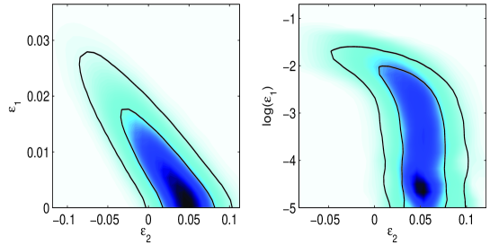
Figure 3: $68\%$ and $95\%$ confidence intervals of the two-dimensional marginalized posteriors in the slow-roll parameters plane, obtained at leading order in the slow-roll expansion MR . The shading is the mean likelihood and the left plot is derived under an uniform prior on $\epsilon_{1}$ while the right panel corresponds to an uniform prior on $\log\epsilon_{1}$.

5 The Classical Limit of Quantum Perturbations

As discussed at length previously, the inflationary cosmological perturbations are of quantum-mechanical origin. However, from the observational point of view, it seems that we deal with a physical phenomenon where quantum mechanics does not play a crucial role (even does not a play a role at all). Therefore, from the conceptual point of view, it is important to understand how the system can become classical GP ; PS ; PSS (see also Ref. CP ). We now turn to this question.

5.1 Coherent States

It seems natural to postulate that a quantum system behaves classically when it is placed in a state such that it follows (exactly or, at least, approximatively) the classical trajectory. For the sake of illustration, let us consider a simple one-dimensional system characterized by the Hamiltonian

$$H(p,q)=\frac{1}{2}p^{2}+V(q)\,,$$ (159)

where, for the moment, the potential $V(q)$ is arbitrary. Solving the classical Hamilton’s equations (given some initial conditions)

$$\frac{{\rm d}p}{{\rm d}t}=-\frac{\partial V(q)}{\partial q}\,,\quad\frac{{\rm d}q}{{\rm d}t}=p\,,$$ (160)

provides the classical solution $p_{\rm cl}$ and $q_{\rm cl}$. At the technical level, the above-mentioned criterion of classicality amounts to choosing a state $|\Psi\rangle$ such that

$$p_{\rm cl}(t)=\langle\Psi|\hat{p}(t)|\Psi\rangle\,,\quad q_{\rm cl}(t)=\langle\Psi|\hat{q}(t)|\Psi\rangle\,.$$ (161)

This is clearly a non-trivial requirement as can be understood from the Ehrenfest theorem. Indeed, this theorem shows that, for any state $|\Psi\rangle$, one has

$$\frac{{\rm d}}{{\rm d}t}\langle\Psi|\hat{p}(t)|\Psi\rangle=-\left\langle\Psi\left|\frac{\partial\hat{V}(q)}{\partial q}\right|\Psi\right\rangle\,,\quad\frac{{\rm d}}{{\rm d}t}\langle\Psi|\hat{q}(t)|\Psi\rangle=\left\langle\Psi\left|\hat{p}\right|\Psi\right\rangle\,,$$ (162)

These equations resemble the Hamilton’s equations (160) but are of course not identical. This implies that, placed in an arbitrary state, the quantum system does not behave classically (i.e. the means of the position and of the momentum do not obey the classical equations). It would be the case only for a state $|\Psi\rangle$ such that

$$\left\langle\Psi\left|\frac{\partial\hat{V}(q)}{\partial q}\right|\Psi\right\rangle=\frac{\partial}{\partial q}V\left(\langle\Psi|\hat{q}|\Psi\rangle\right)\,,$$ (163)

which is not true in general since $\langle\Psi|\hat{q}^{n}|\Psi\rangle\neq\langle\Psi|\hat{q}|\Psi\rangle^{n}$, but obviously satisfied if the potential assumes the particular shape $V(q)\propto q^{2}$, i.e. for the harmonic oscillator. In this case, the means of the position and of the momentum do follow the classical trajectory whatever the state $|\Psi\rangle$ is. This means that Eqs. (161) are in fact not sufficient to define classicality and that one needs to provide extra conditions. It seems natural to require that the wave packet is equally localized in coordinate and momentun $\Delta\hat{q}\equiv\sqrt{\langle\hat{q}^{2}\rangle-\langle\hat{q}\rangle^{2}}=\Delta\hat{p}$ to the minimum allowed by the Heisenberg bound, namely $\Delta\hat{q}\Delta\hat{p}=1/2$. This is another way to define a coherent state, see Eq. (89) which, therefore, represents the “most classical” state of a quantum harmonic oscillator.

We now demonstrate that the state (89) indeed satisfies the above-mentioned properties. If the potential is given by $V(q)=k^{2}q^{2}/2$, then the Hamilton’s equations can be expressed as $\dot{p}=-k^{2}q$ and $\dot{q}=p$ and the “normal variable” variable, see also Eq. (67),

$$\alpha\equiv\sqrt{\frac{k}{2}}\left(q+\frac{i}{k}p\right)\,,$$ (164)

obeys the equation $\dot{\alpha}=-ik\alpha$ which allows us to write the classical trajectory in phase space as

$$p_{\rm cl}(t) = -i\sqrt{\frac{k}{2}}\left(\alpha_{0}{\rm e}^{-ikt}-\alpha_{0}^{*}{\rm e}^{ikt}\right)\,,$$ (165)

$$q_{\rm cl}(t) = \frac{1}{\sqrt{2k}}\left(\alpha_{0}{\rm e}^{-ikt}+\alpha_{0}^{*}{\rm e}^{ikt}\right)\,,$$ (166)

with

$$\alpha_{0}\equiv\sqrt{\frac{k}{2}}\left[q(t=0)+\frac{i}{k}p(t=0)\right]\,,$$ (167)

Let us consider that, at time $t=0$, the system is placed in the state $|\alpha_{0}\rangle$. At time $t>0$, the integration of the Schrödinger equation leads to

$$|\Psi(t)\rangle={\rm e}^{-ikt/2}\left|\alpha(t)=\alpha_{0}{\rm e}^{-ikt}\right\rangle\,.$$ (168)

This result should be understood as follows. In the expression (89) which defines a coherent state, the factor $\alpha$ should be replaced with $\alpha_{0}{\rm e}^{-ikt}$ to get the formula expressing the above state $|\Psi\rangle$. As already mentioned, at the quantum level, the normal variable becomes the annihilation operator [obtained from Eq. (164) by simply replacing $q$ and $p$ with their quantum counter-parts]. This implies

$$\hat{q} = \frac{1}{\sqrt{2k}}\left(\hat{a}+\hat{a}^{\dagger}\right)\,\quad\hat{p}=-i\sqrt{\frac{k}{2}}\left(\hat{a}-\hat{a}^{\dagger}\right)\,.$$ (169)

Then, the crucial step is that any coherent state $|\alpha\rangle$ is the eigenvector of $\hat{a}$ with the eigenvalue $\alpha$, $\hat{a}|\alpha\rangle=\alpha|\alpha\rangle$. Using this property, it is easy to show that, for the state $|\Psi\rangle$ defined by Eq. (168), one has

$$\left\langle\Psi|\hat{p}|\Psi\right\rangle = -i\sqrt{\frac{k}{2}}\left(\alpha_{0}{\rm e}^{-ikt}-\alpha_{0}^{*}{\rm e}^{ikt}\right)\,,$$ (170)

$$\left\langle\Psi|\hat{q}|\Psi\right\rangle = \frac{1}{\sqrt{2k}}\left(\alpha_{0}{\rm e}^{-ikt}+\alpha_{0}^{*}{\rm e}^{ikt}\right)\,.$$ (171)

In the same way, straightforward manipulations lead to

$$\left\langle\Psi|\hat{p}^{2}|\Psi\right\rangle = \frac{k}{2}\left\{1+4\Im^{2}\left[\alpha(t)\right]\right\}\,,\quad\left\langle\Psi|\hat{q}^{2}|\Psi\right\rangle=\frac{1}{2k}\left\{1+4\Re^{2}\left[\alpha(t)\right]\right\}\,,$$ (172)

from which one deduces

$$\Delta\hat{q}=\sqrt{\frac{1}{2k}}\,\quad\Delta\hat{p}=\sqrt{\frac{k}{2}}\,.$$ (173)

We have thus reached our goal, i.e. we have shown that the state (168) follows the classical trajectory and that the quantum dispersion around this trajectory is the same in position and momentum and is minimal (that is to say the Heisenberg inequality is saturated). Therefore, as announced, the coherent state is indeed the “most classical” state. It is also interesting to give the explicit form of the wave-function. It reads

$$\Psi_{\alpha}(q,t)={\rm e}^{i\theta_{\alpha}}\left(\frac{k}{\pi}\right)^{1/4}{\rm e}^{-ikt/2}{\rm e}^{iqp_{\rm cl}(t)}{\rm e}^{-k\left[q-q_{\rm cl}\left(t\right)\right]^{2}/2}\,,$$ (174)

where the phase factor is defined by ${\rm e}^{i\theta_{\alpha}}\equiv{\rm e}^{(\alpha^{*}{}^{2}-\alpha^{2})/4}$.

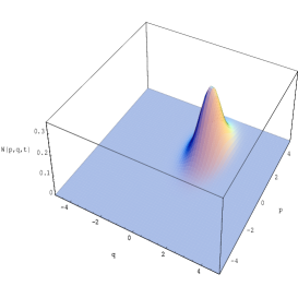
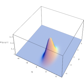
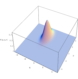
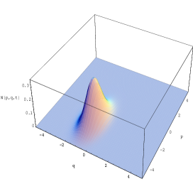
Figure 4: Wigner function (176) for the coherent state $|\alpha\rangle$ at different times. The (arbitrary) values $q_{0}=1$, $p_{0}=1$ and $k=2$ have been used for this figure. This implies $\alpha_{0}=\sqrt{2}{\rm e}^{i\pi/4}$ and, see Eqs. (165), $p_{\rm cl}=2\sqrt{2}\sin\left(\pi/4-t\right)$ and $q_{\rm cl}=\sqrt{2}\cos\left(\pi/4-t\right)$. The upper left panel represents the Wigner function (176) at time $t=0$ while the upper right, lower right and lower left panels correspond to $W(p,q,t)$ at time $t=\pi/2$, $t=\pi$ and $t=3\pi/2$ respectively. The wave packet follows the periodic (ellipsoidal) classical trajectory in phase space and its shape remains unchanged during the motion.

The above expression is defined in real space. However, if one wants to follow the evolution of the system in phase space, it is interesting to introduce the Wigner function wigner ; AA ; SH ; HL defined by the expression (for a one-dimensional system)

$$W\left(q,p,t\right) \equiv \frac{1}{2\pi}\int{\rm d}u\,\Psi^{*}\left(q-\frac{u}{2},t\right){\rm e}^{-ipu}\Psi\left(q+\frac{u}{2},t\right)\,.$$ (175)

A system behaves classically if the Wigner function is positive-definite since, in this case, it can be interpreted as a classical distribution. In addition, if the Wigner function is localized in phase space over a small region corresponding to the classical position and momentum, then the corresponding quantum predictions become indistinguishable from their classical counter-parts and we can indeed state that the system has “classicalized”. For the wave-function (174), the Wigner function can be expressed as

$$W\left(q,p,t\right)=\frac{1}{\pi}{\rm e}^{-k\left[q-q_{\rm cl}(t)\right]^{2}}{\rm e}^{-\frac{1}{k}\left[p-p_{\rm cl}(t)\right]^{2}}\,.$$ (176)

It is represented in Fig. 4. We notice that the Wigner function is always positive and, therefore, according to the above considerations, the system can be considered as classical. Moreover, $W(p,q,t)$ is peaked over a small region in phase space and the wave packet follows exactly the classical trajectory (an ellipse), as is also clear from Eq. (176). This confirms our interpretation of the coherent state as the most classical state.

To conclude this sub-Section, let us notice that the coherent state $|\alpha\rangle$ can be obtained by applying the following unitary operator on the vacuum state

$$|\alpha\rangle={\rm e}^{\alpha a^{\dagger}-\alpha^{*}a}|0\rangle\,.$$ (177)

This equation should be compared to Eqs. (90) and (91). We see that the argument of the exponential is linear in the creation and annihilation operators while it was quadratic in the case of the squeezed state.

5.2 Wigner Function of the Cosmological Perturbations

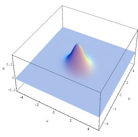
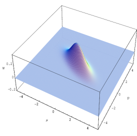
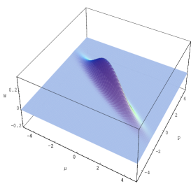
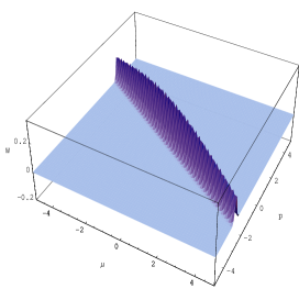
Figure 5: Wigner function of cosmological perturbations obtained from Eq. (179) (for a one-dimensional system). The squeezing parameter $r$ is chosen to be $r=0.1$, $r=0.5$, $r=1$ and $r=2$ for the left upper, right upper, left lower and right lower panels respectively (it is not the same time ordering as in Fig. 4 because, in the present case, the motion is not periodic). The other squeezing parameters are taken to be $\phi=\pi/6$ and $\theta=0$. As can be noticed in this figure, the Wigner function remains positive. Since the squeezing parameter increases with time, the different panels correspond in fact to the Wigner function at different times. At initial time, the quantum state is the vacuum and, therefore, the Wigner function is that of a coherent state, compare the left upper panel with Fig. 4. Then, the Wigner function develops the “Dirac function behavior” discussed in the text that clearly appears on this plot.

In order to study whether the (super-Hubble) cosmological perturbations have “classicalized”, we now use the technical tool of the Wigner function introduced before. The first application to cosmological perturbations was made in Refs. GP ; GS2 . For a two-dimensional system (here, we have in mind $\mu_{\vec{k}}^{{}_{\mathrm{R}}}$ and $\mu_{\vec{k}}^{{}_{\mathrm{I}}}$ for a fixed mode $\vec{k}$), the generalization of Eq. (175) is straightforward and reads

$$W\left(\mu_{\vec{k}}^{{}_{\mathrm{R}}},\mu_{\vec{k}}^{{}_{\mathrm{I}}},p_{\vec{k}}^{{}_{\mathrm{R}}},p_{\vec{k}}^{{}_{\mathrm{I}}}\right) \equiv \frac{1}{\left(2\pi\right)^{2}}\int\int{\rm d}u{\rm d}v\,\Psi^{*}\left(\mu_{\vec{k}}^{{}_{\mathrm{R}}}-\frac{u}{2},\mu_{\vec{k}}^{{}_{\mathrm{I}}}-\frac{v}{2}\right){\rm e}^{-ip_{\vec{k}}^{{}_{\mathrm{R}}}u-ip_{\vec{k}}^{{}_{\mathrm{I}}}v}$$ (178)

$$\times\Psi\left(\mu_{\vec{k}}^{{}_{\mathrm{R}}}+\frac{u}{2},\mu_{\vec{k}}^{{}_{\mathrm{I}}}+\frac{v}{2}\right)\,,$$

where the wave-function is given by the expressions (149). Since we have to deal with Gaussian integrations only, the above Wigner function can be calculated exactly. One obtains

$$W\left(\mu_{\vec{k}}^{{}_{\mathrm{R}}},\mu_{\vec{k}}^{{}_{\mathrm{I}}},p_{\vec{k}}^{{}_{\mathrm{R}}},p_{\vec{k}}^{{}_{\mathrm{I}}}\right) = \Psi\Psi^{*}\frac{1}{2\pi\Re\Omega_{\vec{k}}}\exp\left[\frac{1}{2\Re\Omega_{\vec{k}}}\left(p_{\vec{k}}^{{}_{\mathrm{R}}}+2\Im\Omega_{\vec{k}}\mu_{\vec{k}}^{{}_{\mathrm{R}}}\right)^{2}\right]$$ (179)

$$\times\exp\left[\frac{1}{2\Re\Omega_{\vec{k}}}\left(p_{\vec{k}}^{{}_{\mathrm{I}}}+2\Im\Omega_{\vec{k}}\mu_{\vec{k}}^{{}_{\mathrm{I}}}\right)^{2}\right]\,.$$

It is represented in Fig. 5. The first remark is that the Wigner function is positive (as expected since we deal with a Gaussian state) and, therefore, can be interpreted as a classical distribution. However, as shown in Fig. 5, and contrary to the case of a coherent state, $W$ is not peaked over a small region of phase space. We are interested in the behavior of the Wigner function for modes of astrophysical interest today. These modes have spent time outside the Hubble radius during inflation and, as a consequence, their squeezing parameter $r$ is big. Therefore, it is convenient to express $\Omega_{\vec{k}}$ in terms of the squeezing parameters

$$\Omega_{\vec{k}}=\frac{k}{2}\frac{\cosh r-{\rm e}^{-2i\phi}\sinh r}{\cosh r+{\rm e}^{-2i\phi}\sinh r}\,,$$ (180)

and to take the strong squeezing limit, $r\rightarrow+\infty$. One has

$$\Re\Omega_{\vec{k}}\rightarrow 0\,,\quad\Im\Omega_{\vec{k}}\rightarrow\frac{k}{2}\frac{\sin\phi}{\cos\phi}\,.$$ (181)

This implies

$$W\left(\mu_{\vec{k}}^{{}_{\mathrm{R}}},\mu_{\vec{k}}^{{}_{\mathrm{I}}},p_{\vec{k}}^{{}_{\mathrm{R}}},p_{\vec{k}}^{{}_{\mathrm{I}}}\right) \rightarrow \Psi\Psi^{*}\delta\left(\frac{k}{2}\frac{\sin\phi}{\cos\phi}\mu_{\vec{k}}^{{}_{\mathrm{R}}}+p_{\vec{k}}^{{}_{\mathrm{R}}}\right)\delta\left(\frac{k}{2}\frac{\sin\phi}{\cos\phi}\mu_{\vec{k}}^{{}_{\mathrm{I}}}+p_{\vec{k}}^{{}_{\mathrm{I}}}\right)\,,$$ (182)

where $\delta$ denotes the Dirac function. The above limit is clearly visible in Fig. 5 for $r>1$ (lower panels).

Therefore, in the large squeezing limit, the Wigner function is elongated along a very thin ellipse in phase space. At first sight, this means that the system is not classical since one can not single out a small cell around some classical values $(\mu_{\rm cl},p_{\rm cl})$ that would follow a classical trajectory as it was discussed before. On the other hand, as already mentioned above, the Wigner function remains positive. This means that the interference term which makes the system quantum in the sense that the amplitudes rather than the probabilities should be summed up have become negligible. Therefore, in this sense, the system is classical or, more precisely, is in fact equivalent to a classical stochastic process with a Gaussian distribution (given by the term $\Psi\Psi^{*}$). We see that the nature of this classical limit is quite different to what happens in the case of a coherent state: we cannot predict a definite correlation between position and momentum but we can describe the system in terms of a classical random variable. In practice, this is what is done by astrophysicists: in particular, the quantity $a_{\ell m}$ in Eq. (151) is always treated as a Gaussian random variable and any detailed quantum-mechanical considerations avoided.

As argued in Ref. PS , the system has become classical (in the sense explained before) without any need to take into account its interaction with the environment. This is “decoherence without decoherence” as stressed in the above-refered article. More on this subtle issue can be found in Refs. PS ; KP . Of course, the question of whether the wave-function of the perturbation has collapsed or not (and the question of whether this question is meaningful in the present context and/or dependent on the interpretation of quantum mechanics that one chooses to consider) is even more delicate PSS and we will not touch upon this issue here.

5.3 Wigner function of a Free Particle

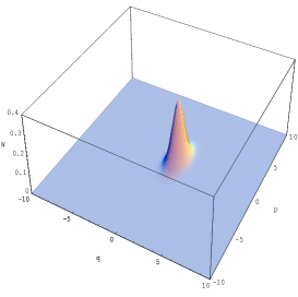
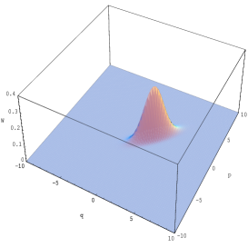
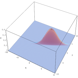
Figure 6: Wigner function (188) of a free particle. The parameters chosen are $k_{0}=1$, $q_{0}=1$ and $a=1$ which is in fact equivalent to considering the dimensionless quantities $ap$, $q/a$ and $t/a^{2}$. The left upper panel corresponds to $t/a^{2}=0$ while the right upper, left lower and right lower panels represent the Wigner function at times $t/a^{2}=0.8,2,3$ respectively (here, the time ordering is similar to that in Fig. 5 and, therefore, different from that in Fig. 4). Initially, the wave packet is well-localized in phase space and, as time goes on, the spreading of the wave packet becomes apparent.

We now consider the case of a free particle since it shares common points with the case of cosmological perturbations as first noticed in Ref. KP . At the beginning of this section, we mentioned that, in the particular case of the harmonic oscillator $V(q)\propto q^{2}$, the quantum mean value of the position and momentum operators always follow the classical trajectory whatever the quantum state $|\Psi\rangle$ in which the system is placed. There is obviously another situation where this is also the case: the free massive particle where $V(q)=0$. The wave-function is given by (we take $m=1$)

$$\Psi(q,t) = \left(\frac{2a^{2}}{\pi}\right)^{1/4}\frac{1}{\left(a^{4}+4t^{2}\right)^{1/4}}{\rm e}^{-i\tan^{-1}\left(2t/a^{2}\right)/2+ik_{0}(q-q_{0})-ik_{0}^{2}t/2}$$ (183)

$$\times{\rm e}^{-\left(q-q_{0}-k_{0}t\right)^{2}/\left(a^{2}+2it\right)}\,,$$

where we have assumed to the wave packet is centered at $q=q_{0}$ at $t=t_{0}$. The parameter $a$ represents the width of the wave packet while $k_{0}$ parameterizes its velocity. The means of $\hat{p}$ and $\hat{q}$ can be expressed as

$$\langle\hat{p}\rangle=k_{0}=p_{\rm cl}\,,\quad\langle\hat{q}\rangle=q_{0}+k_{0}t=q_{\rm cl}\,.$$ (184)

Therefore, as announced, they follow exactly the classical trajectory. But, as argued in the sub-Section devoted to coherent states, one must also compute the dispersions. Straightforward calculations lead to

$$\left\langle\hat{p}^{2}\right\rangle = k_{0}^{2}+\frac{1}{a^{2}}\,,\quad\left\langle\hat{q}^{2}\right\rangle=\frac{1}{4a^{2}}\left(a^{4}+4t^{2}\right)+\left(q_{0}+k_{0}t\right)^{2}\,,$$ (185)

from which one deduces that

$$\Delta\hat{p}=\frac{1}{a}\,,\quad\Delta\hat{q}=\frac{a}{2}\sqrt{1+4\frac{t^{2}}{a^{4}}}\,.$$ (186)

At $t=0$, one has $\Delta\hat{q}\Delta\hat{p}=1/2$ and the Heisenberg bound is saturated: at initial time, the wave packet is minimal. But then, and contrary to the case of the harmonic oscillator, the dispersion on the position is increasing with time (while the dispersion on the momentum remains constant). The wave packet does not keep its shape unchanged while moving as it was the case for a potential $V(q)\propto q^{2}$. This is the well-known phenomenon dubbed “spreading of the wave packet”. However, it exists a quasi-classical interpretation of this situation. Indeed, when $t\gg a^{2}$, one has

$$\Delta\hat{q}\sim\frac{t}{a}=\Delta\hat{p}\,t=\Delta v_{\rm cl}t\,,$$ (187)

which reproduces the classical motion. On the contrary, for small times, $\Delta\hat{q}$ must take values very different from the classical ones in order to satisfy the Heisenberg inequality. Therefore, in the regime $t\gg a^{2}$, the system is classical but in a sense slightly different from the one encountered in the harmonic oscillator case.

Let us now calculate the Wigner function of the free particle. One obtains

$$W(p,q,t) = \frac{1}{\pi}\exp\left[-\frac{2a^{2}}{a^{4}+4t^{2}}\left(q-q_{\rm cl}\right)^{2}\right]$$ (188)

$$\times \exp\left\{-\frac{a^{4}+4t^{2}}{2a^{2}}\left[p-p_{\rm cl}-\frac{4t}{a^{4}+4t^{2}}\left(q-q_{\rm cl}\right)\right]^{2}\right\}\,.$$

This equation is similar to Eq. (179). The Wigner function is the product of one exponential factor whose argument is proportional to “ $\left(q-q_{\rm cl}^{2}\right)$” [hidden in the term $\Psi^{*}\Psi$ in Eq. (179)] and of another exponential term whose argument has the form “$\left[p-p_{\rm cl}-f(t)\left(q-q_{\rm cl}\right)\right]^{2}$, where $f(t)$ is a function of time only. Therefore, the classical limit of cosmological perturbations can also be understood in terms of the (quasi-) classical limit of a free particle, as discussed in the previous paragraph.

The Wigner function (188) is represented in Fig. 6. This plot confirms the interpretation presented above. First of all, the Wigner function remains positive which indicates that a classical interpretation is meaningful. At initial time, the Wigner function is well-localized because the wave packet is minimal. Then, at time goes on, the spreading of the wave packet causes the spreading of the Wigner function in phase space. Clearly, this case bears some ressemblence with that of cosmological perturbations, compare Figs. 5 and 6. Therefore, inflationary fluctuations on large scales become classical in the same sense that a free particle is classical far from the origin. A much more detailed description of this analogy can be found in Ref. KP .

6 Conclusions

In this review, we have presented a pedagogical introduction to the theory of inflationary cosmological perturbations of quantum-mechanical origin, focusing mainly on its fundamental aspects. We have shown that the mechanism responsible for the production of the initial fluctuations in the early universe is in fact similar to a well-known effect in quantum field theory, namely the Schwinger effect. It is indeed the “interaction” of the quantum perturbed metric $\delta g_{\mu\nu}$ (and of the perturbed inflaton field $\delta\varphi$) with the background gravitational field which is responsible for the amplification of the initial vacuum fluctuations in the same way that pair creation can occur in an external electrical field. Because the gravitational field in the early universe can be strong (in Planck units), this mechanism leads to observable effects, in particular to CMB temperature fluctuations. Therefore, these fluctuations originate from a remarkable interplay between general relativity and quantum mechanics.

There is also another aspect associated with the inflationary mechanism discussed above that could be relevant to probe fundamental physics. In a typical model of inflation, the total number of e-folds is such that the scales of astrophysical interest today were initially not only smaller than the Hubble radius but also smaller than the Planck (or string) scale. As a consequence, the WKB initial conditions discussed before are maybe modified by quantum gravity (stringy) effects and, therefore, this opens up the possibility to probe these effects through observations of the CMB BM1 ; MR2 . Of course, an open issue is the fact that it is difficult to calculate how quantum gravity/string theory will affect the initial conditions. Nevertheless, it is possible to draw some generic conclusions. Firstly, the standard initial condition consists in choosing only one WKB branch. Hence, any modification amounts to considering that the second branch is present. As a consequence, super-imposed oscillations in the power spectrum unavoidably appear, the amplitude and the frequency of these oscillations being unfortunately model dependent BM1 (for the observational status of these oscillations, see Refs. MR2 ; MR ). Secondly, the presence of the second WKB branch means, in some sense, the presence of particles in the initial state and, therefore, there is potentially a back-reaction problem. Generically, the larger the amplitude of the super-imposed oscillations is, the more severe the back-reaction issue. On the other hand, predicting the effect of the energy density of the perturbations is difficult and it is not clear whether this will spoil inflation or, for instance, just renormalize the cosmological constant BM2 ; danielsson . These problems are still open questions but it is interesting to notice that the inflationary scenario is rich enough to provide yet another means to learn about fundamental physics.

References

- (1) A. Guth: Phys Rev D 23, 347 (1981).
- (2) A. Linde: Phys Lett B 108, 389 (1982); A. Albrecht and P. J. Steinhardt: Phys Rev Lett 48, 1220 (1982); A. Linde: Phys Lett B 129, 177 (1983).
- (3) V. Mukhanov and G. Chibisov: JETP Lett 33, 532 (1981); Sov Phys JETP 56, 258 (1982).
- (4) S. Hawking: Phys Lett 115B, 295 (1982); A. Starobinsky: Phys Lett 117B, 175 (1982); A. Guth and S. Y. Pi: Phys Rev Lett 49, 1110 (1982); J. M. Bardeen, P. J. Steinhardt and M. S. Turner: Phys Rev D 28, 679 (1983).
- (5) D. N. Spergel et al.: astro-ph/0603449; C. L. Bennet et al.: Astrophys J Suppl 148, 1 (2003), astro-ph/0302207; G. Hinshaw et al.: Astrophys J Suppl 148, 135 (2003), astro-ph/0302217; L. Verde et al.: Astrophys J Suppl 148, 195 (2003), astro-ph/0302218; H. V. Peiris et al.: Astrophys J Suppl 148, 213 (2003), astro-ph/0302225.
- (6) J. Schwinger: Phys Rev 82, 664 (1951).
- (7) A. Ringwald: hep-ph/0112254.
- (8) R. Alkofer, M. B. Hecht, C. D. Roberts, S. M. Schmidt and D. V. Vinnik: Phys Rev Lett 87, 193902 (2001), nucl-th/0108046.
- (9) Point of the scientific case in the XFEL-STI Interim Report of January 11, 2005 available at http://xfel.desy.de/science/index_eng.html
- (10) http://www-ssrl.slac.stanford.edu/lcls/
- (11) V. F. Mukhanov, H. A. Feldman and R. H. Brandenberger: Phys Rep 215, 203 (1992).
- (12) A. Guth and S. Pi: Phys Rev D 32, 1899 (1985).
- (13) D. Polarski and A. Starobinsky: Class. Quantum Grav. 13, 377 (1996), gr-qc/9504030.
- (14) W. Zurek: Phys Rev D 26, 1862 (1982).
- (15) E. Wigner: Phys Rev 40, 749 (1932).
- (16) J. Martin: Proceedings of the XXIV Brazilian National Meeting on Particles and Fields, Caxambu, Brazil, (2004), astro-ph/0312492.
- (17) J. Martin: Lect Notes Phys 669, 199 (2005), hep-th/0406011.
- (18) E. Ince: Ordinary Differential Equations (Dover, 1926).
- (19) C. Kiefer: Phys Rev D 45, 2044 (1992).
- (20) K. Srinivasan and T. Padmanabhan: gr-qc/9807064.
- (21) I. S. Gradshteyn and I. M. Ryzhik: Tables of Integrals, Series and Products (Academic, New York, 1981).
- (22) E. Brezin and C. Itzykson: Phys Rev D 2, 1191 (1970).
- (23) H. M. Fried, Y. Gabellini, B. H. McKellar and J. Avan: Phys Rev D 63, 125001 (2001).
- (24) J. Avan, H. M. Fried and Y. Gabellini: Phys Rev D 67, 016003 (2003), hep-th/0208053.
- (25) H. M. Fried and Y. Gabellini: Phys Rev D 73, 011901 (2006), hep-th/0510233.
- (26) M. Turner: Phys Rev D 28, 1243 (1983).
- (27) L. Kofman, A. Linde and A. Starobinsky: Phys Rev D 56, 3258 (1997), hep-ph/9704452.
- (28) C. Cohen-Tannoudji, J. Dupont-Roc and G. Grynberg: Photons et atomes, Introduction a l’électrodynamique quantique, (Editions du CNRS, 1987).
- (29) H. Goldstein: Classical Mechanics, (Addisson-Wesley, 1990).
- (30) J. M. Cervero and A. Rodriguez: International Journal of Theoretical Physics 41, 503 (2002), quant-ph/0106157.
- (31) P. Peter, E. Pinho and N. Pinto-Neto: JCAP 0507, 014 (2005), hep-th/0509232.
- (32) L. P. Grishchuk and Y. V. Sidorov: Class. Quantum Grav. 6, L155 (1989).
- (33) L. P. Grishchuk and Y. V. Sidorov: Phys Rev D 42, 3413 (1990).
- (34) L. P. Grishchuk, H. A. Hauss and K. Bergman: Phys Rev D 46, 1440 (1992).
- (35) A. Albrecht, P. Ferreira, M. Joyce and T. Prokopec: Phys Rev D 50, 4807 (1994), astro-ph/9303001.
- (36) B. L. Schumacher: Phys Rep 135, 317 (1986).
- (37) W. Schleich, D. F. Walls and J. A. Wheeler: Phys Rev A 38, 1177 (1988).
- (38) C. Kiefer and D. Polarski: gr-qc/9805014.
- (39) A. Mostafazadeh: quant-ph/9612038.
- (40) Haewon Lee and W. S. l’Yi: Phys Rev A 51, 982 (1995), hep-th/9406106.
- (41) Y. S. Kim and E. P. Wigner: Am J Phys 58, 439 (1990).
- (42) A. Ogura and M. Sekiguchi: quant-ph/0410173.
- (43) J. A. Bardeen: Phys Rev D 22, 1882 (1980).
- (44) D. H. Lyth: Phys Rev D 31, 1792 (1985).
- (45) J. Martin and D. J. Schwarz: Phys Rev D 57, 3302 (1998), gr-qc/9704049.
- (46) D. Lyth and A. Riotto: Phys Rept 314, 1 (1999), hep-ph/9807278.
- (47) R. Kallosh: this volume.
- (48) L. P. Grishchuk: Zh. Eksp. Teor. Fiz 67, 825 (1974).
- (49) E. D. Stewart and D. H. Lyth: Phys. Lett. B302, 171 (1993).
- (50) J. Martin and D. J. Schwarz: Phys Rev D 62, 103520 (2000), astro-ph/9911225; J. Martin, A. Riazuelo and D. J. Schwarz: Astrophys J 543, L99 (2000), astro-ph/0006392.
- (51) S. Leach, A. R. Liddle, J. Martin and D. J. Schwarz: Phys Rev D 66, 023515 (2002), astro-ph/0202094.
- (52) D. J. Schwarz, C. A. Terrero-Escalante and A. A. Garcia: Phys. Lett B517, 243 (2001), astro-ph/0106020.
- (53) J. Martin and D. J. Schwarz: Phys Rev D 67, 083512 (2003), astro-ph/0210533.
- (54) H. A. Kramers: Zeit f Physik 39, 836 (1926).
- (55) L. A. Young and G. E. Uhlenbeck: Phys Rev 36, 1158 (1930).
- (56) R. E. Langer: Phys Rev 51, 669 (1937).
- (57) R. Casadio, F. Finelli, M. Luzzi and G. Venturi: Phys Rev D 72, 103516 (2005), gr-qc/0510103.
- (58) R. K. Sachs and A. M. Wolfe: Astrophys J 147, 73 (1967).
- (59) M. Panek: Phys Rev D 49, 648 (1986).
- (60) L. P. Grishchuk and J. Martin: Phys Rev D 56, 1924 (1997), gr-qc/9702018.
- (61) J. Martin and C. Ringeval: JCAP 0608, 009 (2006), astro-ph/0605367.
- (62) C. Ringeval: this volume.
- (63) A. Perez, H. Sahlmann and D. Sudarsky: Class. Quantum Grav. 23, 2317 (2006), gr-qc/0508100.
- (64) D. Campo and R. Parentani: Phys Rev D 74, 045015 (2005), astro-ph/0505376.
- (65) A. Anderson: Phys Rev D 42, 585 (1990).
- (66) S. Habib: Phys Rev D 42, 2566 (1990).
- (67) S. Habib and R. Laflamme: Phys Rev D 42, 4056 (1990).
- (68) J. Martin and R. Brandenberger: Phys Rev D 63, 123501 (2001), hep-th/0005209; R. Brandenberger and J. Martin: Mod Phys Lett A16, 999 (2001), astro-ph/0005432; R. Brandenberger, S. Joras and J. Martin: Phys Rev D 66, 083514 (2002), hep-th/0112122; J. Martin and R. Brandenberger: Phys Rev D 68, 063513 (2003), hep-th/0305161.
- (69) J. Martin and C. Ringeval: Phys Rev D 69, 083515 (2004), astro-ph/0310382; J. Martin and C. Ringeval: Phys Rev D 69, 127303 (2004), astro-ph/0402609; J. Martin and C. Ringeval: JCAP 0501, 007 (2005), hep-ph/0405249.
- (70) J. Martin and R. Brandenberger: Phys Rev D 71, 023504 (2005), hep-th/0410223.
- (71) U. Danielsson: JCAP 0603, 014 (2006), hep-th/0511273.