Inflation after WMAP3: Confronting the Slow-Roll and Exact Power Spectra with CMB Data

Abstract

The implications of the WMAP (Wilkinson Microwave Anisotropy Probe) third year data for inflation are investigated using both the slow-roll approximation and an exact numerical integration of the inflationary power spectra including a phenomenological modelling of the reheating era. At slow-roll leading order, the constraints $\epsilon_{1}<0.022$ and $-0.07<\epsilon_{2}<0.07$ are obtained at $95\%$ CL (Confidence Level) implying a tensor-to-scalar ratio $r_{10}<0.21$ and a Hubble parameter during inflation $H/m_{\scriptscriptstyle{\mathrm{Pl}}}<1.3\times 10^{-5}$. At next-to-leading order, a tendency for $\epsilon_{3}>0$ is observed. With regards to the exact numerical integration, large field models, $V(\phi)\propto\phi^{p}$, with $p>3.1$ are now excluded at $95\%$ CL. Small field models, $V(\phi)\propto 1-(\phi/\mu)^{p}$, are still compatible with the data for all values of $p$. However, if $\mu/m_{\scriptscriptstyle{\mathrm{Pl}}}<10$ is assumed, then the case $p=2$ is slightly disfavoured. In addition, mild constraints on the reheating temperature for an extreme equation of state $w_{\mathrm{reh}}\gtrsim-1/3$ are found, namely $T_{\mathrm{reh}}>2\,\mbox{TeV}$ at $95\%$ CL. Hybrid models are disfavoured by the data, the best fit model having $\Delta\chi^{2}\simeq+5$ with two extra parameters in comparison with large field models. Running mass models remain compatible, but no prior independent constraints can be obtained. Finally, superimposed oscillations of trans-Planckian origin are studied. The vanilla slow-roll model is still the most probable one. However, the overall statistical weight in favour of superimposed oscillations has increased in comparison with the WMAP first year data, the amplitude of the oscillations satisfying $2|x|\sigma_{0}<0.76$ at $95\%$ CL. The best fit model leads to an improvement of $\Delta\chi^{2}\simeq-12$ for $3$ extra parameters. Moreover, compared to other oscillatory patterns, the logarithmic shape is favoured.

1 Introduction

The recent release of the three years WMAP data [1, 2, 3, 4] constitutes an important step for the theory of inflation. One now has at our disposal high accuracy data that can be used to probe the details of the inflationary scenario and to learn about the physical conditions that prevailed in the very early universe, at very high energies comparable to the Grand Unified Theory (GUT) scale. There are many aspects that would be interesting to study but, clearly, in a first approach, one can restrict ourselves to (effective) single field models and see whether it is already possible to constrain the shape of the inflaton potential $V(\phi)$. In particular, it is important to known whether it is necessary to go beyond a simple Harrison-Zeldovitch (scale-invariant) power spectrum to correctly fit the data. If so, as indicated by the results of reference [2] and from a model building point of view, this means that the inflaton potential is not completely flat and/or that inflation is not driven by a pure cosmological constant. Equivalently, this also means that the observations start feeling the non-trivial shape of the potential. In this case, a non-vanishing second order derivative of the potential is seen while the first order derivative of $V(\phi)$ presumably remains unconstrained from below since, otherwise, primordial gravitational waves would have been detected. Besides the previous issue, one would also like to go further and to study which inflationary models remain compatible with the data and which ones are ruled out. Addressing these questions is the main goal of this article. Notice that we restrict our considerations to WMAP3 data only although including other data sets could allow us to obtain tighter constraints on the inflationary models studied here. In a first step, we think it is more reasonable to proceed this way in order not to mix the effects of using different data sets with those originating from the new numerical approach introduced in this article.

To deal with this problem we proceed as follow. We first use the slow-roll approximation and derive the constraints put by the third year WMAP data on the first three slow-roll parameters (i.e. second order slow-roll approximation). Then, we compute exactly these parameters for the large field, small field, hybrid and running mass models. In particular, we show that some widely used approximate expressions for $\epsilon_{1}$ and $\epsilon_{2}$ are no longer sufficient to assess the likelihood of some models (small field models) given the quality of the data. For this reason, in this article, we always evaluate exactly the slow-roll parameters, using simple numerical methods if necessary. The implications of the WMAP3 data using a slow-roll prior have also been investigated in references [5, 6, 7, 8, 9].

In a second step, one frees ourselves from any approximation (except the linear theory of cosmological perturbations) and calculate the power spectra exactly by means of numerical computations. The models that we study are the same than the ones already mentioned for the slow-roll case, namely large field, small field, hybrid and running mass models. These exact power spectra are computed mode by mode and fed into a modified Cosmic Background Microwave (CMB) code, here a modified CAMB code [10], which allows us to determine the temperature and polarisation multipole moments. Finally, we explore the corresponding parameters space by using Monte-Carlo techniques as implemented in the COSMOMC code [11] together with the likelihood code developed by the WMAP team [2]. This allows us to put constraints on the free parameters characterising the models during the inflationary phase but also, in principle, during the reheating phase although, most of the time, the accuracy of the data is not sufficient to obtain relevant limits on the reheating temperature.

This article is organised as follows. In section 2, we briefly recall some basic facts about inflation, reheating and the theory of inflationary cosmological perturbations of quantum-mechanical origin. Section 3 is devoted to the slow-roll approximation. In subsection 3.1, the derivation of the slow-roll scalar and tensor power spectra is recalled. In subsection 3.2, we present the WMAP data constraints on the slow-roll parameters at first order (i.e. $\epsilon_{1}$ and $\epsilon_{2}$) and also at second order (i.e. the two previous ones plus $\epsilon_{3}$). In subsections 3.3 to 3.6, we calculate the slow-roll parameters for the large field, small field, hybrid and running mass inflationary models. These results are then compared to the constraints on $\epsilon_{1}$, $\epsilon_{2}$ and $\epsilon_{3}$ obtained previously. Section 4 is devoted to the the exact computations of the inflationary power spectra for the four models mentioned above. In subsection 4.1, we briefly describe the method and the code used to perform the numerical calculations. In subsections 4.2 to 4.5, the exact numerical results are used to discuss the constraints put by the third year WMAP data on the free parameters describing the models but also (when possible) on the subsequent reheating phase. Finally, in section 5, we investigate the presence of superimposed oscillations in the CMB multipoles. In subsection 5.1, we discuss a possible physical origin for those oscillations, namely trans-Planckian effects during inflation. This allows us to use a well-motivated and well-defined shape for the oscillatory power spectra. Then, in subsection 5.2, we compare these spectra to the third year WMAP data and use them to put constraints on the amplitude, the frequency and the phase of the superimposed oscillations. In the last section 6, we recap our findings and present our conclusions.

2 Basics of inflation

2.1 The background

2.1.1 The accelerated phase

In this section, in order to describe the general setting and to fix our notations, we recall some basic and well-known facts about inflation at the background and perturbed levels. A phase of inflation is supposed to make the universe homogeneous and isotropic on large scales. It also drastically reduces its spatial curvature in agreement with the observations which indicate that the spatial sections are extremely flat. As a consequence, the metric tensor which describes the geometry of the Universe can be taken of the Friedman-Lemaître-Robertson-Walker (FLRW) form, namely

$$\mathrm{d}s^{2}=-\mathrm{d}t^{2}+a^{2}(t)\delta_{ij}\mathrm{d}x^{i}\mathrm{d}x^{j}=a^{2}(\eta)\left(-\mathrm{d}\eta^{2}+\delta_{ij}\mathrm{d}x^{i}\mathrm{d}x^{j}\right),$$ (1)

where $\delta_{ij}$ is the Krönecker symbol. The variable $t$ is the cosmic time while $\eta$ is the conformal time and these two quantities are related by $\mathrm{d}t=a\mathrm{d}\eta$. In the following, both will be used, the choice of using one rather than the other being made for convenience only and according to the problem at hand. Another important time variable is the number of e-folds defined by the following expression

$$N\equiv\ln\left(\frac{a}{a_{\mathrm{in}}}\right),$$ (2)

where $a_{\mathrm{in}}$ is the value of the scale factor at some initial time. As required to solve the flatness and homogeneity issue of the FLRW model, the total number of e-folds during inflation must be greater than $60$.

The evolution of $a(\eta)$, the only free function in the above metric element, is controlled by the Einstein equations. If matter is assumed to be a perfect fluid, they read

$$\frac{3}{a^{2}}\left(\frac{a^{\prime}}{a}\right)^{2}=\frac{8\pi}{m_{\scriptscriptstyle{\mathrm{Pl}}}^{2}}\rho\,,\qquad-\frac{1}{a^{2}}\left[2\frac{a^{\prime\prime}}{a}-\biggl{(}\frac{a^{\prime}}{a}\biggr{)}^{2}\right]=\frac{8\pi}{m_{\scriptscriptstyle{\mathrm{Pl}}}^{2}}P\,,$$ (3)

where a prime denotes a derivative with respect to conformal time and $\rho$, $P$ are respectively the energy density and the pressure of the cosmological fluid driving the dynamics of the universe. In the following, we will use the conformal Hubble parameter defined by $\mathcal{H}\equiv a^{\prime}/a$. In addition, one also has the energy conservation equation

$$\rho^{\prime}+3{\cal H}(\rho+P)=0\,,$$ (4)

which can also be obtained from the Einstein equations by means of the Bianchi identities.

By definition, inflation is a phase of accelerated expansion for which the scale factor satisfies [12, 13, 14, 15]

$$\frac{\mathrm{d}^{2}a}{\mathrm{d}t^{2}}>0\,,$$ (5)

and this condition can also be re-written as

$$\epsilon_{1}(\eta)\equiv 1-\left(\frac{a}{a^{\prime}}\right)^{2}\left(\frac{a^{\prime}}{a}\right)^{\prime}<1\,.$$ (6)

The quantity $\epsilon_{1}$ is in fact nothing but the first Hubble-flow (or slow-roll) parameter $-\dot{H}/H^{2}$ where $H=\mathcal{H}/a$ denotes the physical Hubble parameter (see below). Inflation stops when $\epsilon_{1}=1$. Another way to express the acceleration of the scale factor is to combine equations (3). One gets

$$\frac{\ddot{a}}{a}=-\frac{4\pi}{3m_{\scriptscriptstyle{\mathrm{Pl}}}^{2}}\left(\rho+3P\right),$$ (7)

where a dot denotes a derivative with respect to the cosmic time $t$. Clearly, inflation can be obtained if the fluid dominating the universe has a negative pressure such that $P<-\rho/3$.

A possible implementation of the inflationary scenario is to assume that the matter content of the universe is described by a scalar field $\phi(\eta)$ with a potential $V(\phi)$ since, when $V(\phi)$ is sufficiently flat, the effective pressure of the scalar field can be negative [12, 13, 16, 14, 15]. In this article, we restrict ourselves to the case of a single scalar field. In this case, the two Einstein equations take the form

$$\frac{3}{a^{2}}\mathcal{H}^{2}=\frac{8\pi}{m_{\scriptscriptstyle{\mathrm{Pl}}}^{2}}\left[\frac{1}{2}\frac{(\phi^{\prime})^{2}}{a^{2}}+V(\phi)\right],$$ (8)

and

$$-\frac{1}{a^{2}}\left(2\mathcal{H}^{\prime}+\mathcal{H}^{2}\right)=\frac{8\pi}{m_{\scriptscriptstyle{\mathrm{Pl}}}^{2}}\left[\frac{1}{2}\frac{(\phi^{\prime})^{2}}{a^{2}}-V(\phi)\right].$$ (9)

Using the expressions of $\rho$ and $P$ for a scalar field, the conservation equation (4) reduces to the Klein-Gordon equation written in a FLRW background, namely

$$\phi^{\prime\prime}+2\mathcal{H}\phi^{\prime}+a^{2}\frac{\mathrm{d}V(\phi)}{\mathrm{d}\phi}=0\,.$$ (10)

This equation can also be directly derived from (8) and (9). In fact, the physical interpretation is made easier if the Klein-Gordon equation is written in terms of the number of e-folds, namely [17]

$$\frac{1}{3-\epsilon_{1}}\frac{{\mathrm{d}}^{2}\phi}{{\mathrm{d}}N^{2}}+\frac{{\rm d}\phi}{{\mathrm{d}}N}=-\frac{m_{\scriptscriptstyle{\mathrm{Pl}}}^{2}}{8\pi}\frac{{\mathrm{d}}\ln V(\phi)}{{\mathrm{d}}\phi}\,.$$ (11)

We see that studying the evolution of the scalar field is in fact equivalent to study the motion of particle in an effective potential $\ln V(\phi)$ with a slightly variable mass and a constant friction term. This is the reason why, in the following, when we consider concrete models, we will also pay attention to the logarithm of the potential in order to gain intuition about how inflation proceeds.

If we are given a model, that is to say a concrete form for the potential $V(\phi)$, then the equations of motion can be integrated from the initial conditions $\phi_{\mathrm{in}}$ and $\phi_{\mathrm{in}}^{\prime}$. In general, the shape of the potentials that we consider does not allow simple analytical solutions of the Einstein equations. In that case, one has to rely on analytical approximations of numerical calculations. However, the following potential [18]

$$V(\phi)=M^{4}\exp\left[-\frac{4\sqrt{\pi}}{m_{\scriptscriptstyle{\mathrm{Pl}}}}\sqrt{\frac{2+\beta}{1+\beta}}\left(\phi-\phi_{\mathrm{in}}\right)\right]\,,$$ (12)

is an example where the exact integration can be performed analytically. One obtains power-law inflation for which the scale factor and the scalar field are respectively given by

$$a(\eta)=\ell_{0}|\eta|^{1+\beta}\,,\qquad\phi=\phi_{\mathrm{in}}+\frac{m_{\scriptscriptstyle{\mathrm{Pl}}}}{2}\sqrt{\frac{2+\beta}{\pi(1+\beta)}}(1+\beta)\ln|\eta|\,.$$ (13)

In this model the parameter $\epsilon_{1}$ is given by $\epsilon_{1}=(2+\beta)/(1+\beta)$ and, therefore, inflation occurs if $\beta<-2$ (we do not consider the case where $-2<\beta<-1$ which cannot be realised with a single scalar field). However, this model is not a satisfactory model, since inflation never stops, at least if one does not use another mechanism.

2.1.2 The end of inflation

When an exact integration is performed, it is very important to have a description of the reheating phase. Without such a description, one cannot relate the physical scales today to the physical scales during inflation simply because one does not know the entire history of the universe. As mentioned before, inflation ends for $\phi=\phi_{\mathrm{end}}$, or $\rho=\rho_{\mathrm{end}}$ (or again for $H=H_{\mathrm{end}}$), when $\epsilon_{1}=1$. The difficulty is that the process of reheating can be model dependent. For the large field inflation models, one may use a phenomenological description based on the fact that the potential is given by $V(\phi)\propto\phi^{p}$. In this case, after the end of inflation, the field starts oscillating around its minimum [19, 20]. In this regime, one can show that the average energy density behaves as $\rho_{\mathrm{inf}}\propto a^{-6p/(p+2)}$ and, as a result, the scale factor is given by $a(t)\propto t^{(p+2)/(3p)}$. In other words, the equation of state $P=w\rho$ during reheating has a constant state parameter given by

$$w_{\mathrm{reh}}=\frac{p-2}{p+2}\,.$$ (14)

For a massive scalar field, $p=2$, the energy density evolves as in a matter-dominated epoch while for a quartic potential, $p=4$, the energy density behaves as in radiation-dominated era. Nevertheless, one always has

$$-\frac{1}{3}<w_{\mathrm{reh}}<1\,,$$ (15)

for $p>1$.

The previous considerations and the description of the oscillatory phase were just based on the Klein-Gordon equation (10). It is clear that, with this equation only, the decay of the inflaton field into radiation cannot be described. In order to take into account this effect, it is common to phenomenologically add a friction term $\Gamma\dot{\phi}$ in the Klein-Gordon equation which now reads [19]

$$\ddot{\phi}+3H\dot{\phi}+\Gamma\dot{\phi}+\frac{{\rm d}V(\phi)}{{\mathrm{d}}\phi}=0\,.$$ (16)

In fact, this description cannot account for the complexity of the reheating stage [20, 21, 22, 23, 24, 25, 26, 27, 28, 29, 30]. But for our purpose, the above treatment will be sufficient. Since we have modified the Klein-Gordon equation one should also modify the conservation equation for the radiation energy density in order to ensure the total energy conservation:

$$\dot{\rho}_{\mathrm{rad}}=-4H\rho_{\mathrm{rad}}+\Gamma\rho_{\mathrm{inf}}\,.$$ (17)

In fact, the previous discussion can be generalized to other inflationary models by simply assuming that the reheating era takes place with a constant state parameter $w_{\mathrm{reh}}$ for which $a\propto t^{2/(3+3w_{\mathrm{reh}})}$ and $\rho\propto a^{-3-3w_{\mathrm{reh}}}$. Note however that unlike for the large field models, this parameter is not necessarily related to the inflationary potential and equation (14) is generally not satisfied. However, the equations for $\rho_{\mathrm{inf}}$ and $\rho_{\mathrm{rad}}$ can be exactly integrated and the solutions read [14]

$$\rho_{\mathrm{inf}}(t) = \rho_{\mathrm{end}}\left(\frac{a}{a_{\mathrm{end}}}\right)^{-3(1+w_{\mathrm{reh}})}\exp\left[-\left(1+w_{\mathrm{reh}}\right)\Gamma\left(t-t_{\mathrm{end}}\right)\right],$$ (18)

$$\rho_{\mathrm{rad}}(t) = \Gamma t_{\mathrm{end}}\rho_{\mathrm{end}}\left(\frac{a_{\mathrm{end}}}{a}\right)^{4}\left[\left(1+w_{\mathrm{reh}}\right)\Gamma t_{\mathrm{end}}\right]^{(3w_{\mathrm{reh}}-5)/(3+3w_{\mathrm{reh}})}$$ (19)

$$\times \exp\left[\left(1+w_{\mathrm{reh}}\right)\Gamma t_{\mathrm{end}}\right]\left\{\gamma\left[\frac{5-3w_{\mathrm{reh}}}{3+3w_{\mathrm{reh}}},\left(1+w_{\mathrm{reh}}\right)\Gamma t\right]\right.$$

$$- \left.\gamma\left[\frac{5-3w_{\mathrm{reh}}}{3+3w_{\mathrm{reh}}},\left(1+w_{\mathrm{reh}}\right)\Gamma t_{\mathrm{end}}\right]\right\},$$

where $t=t_{\mathrm{end}}$ is the time at which the oscillations start (i.e. the time at which inflation ends). The function $\gamma(\alpha,x)$ is the incomplete gamma function [31, 32] defined by $\gamma(\alpha,x)\equiv\int_{0}^{x}{\mathrm{e}}^{-t}t^{\alpha-1}{\mathrm{d}}t$. It was shown in Ref. [14] that the expression of $\rho_{\mathrm{rad}}$ can be simplified if one uses the expression of the incomplete gamma function for small values of its argument. For times $t>t_{\mathrm{end}}$ with $t_{\mathrm{end}}\ll t_{\mathrm{reh}}$ where $t_{\mathrm{reh}}\equiv\Gamma^{-1}$, one obtains the solution [19]

$$\rho_{\mathrm{rad}}(t)\simeq\Gamma t\rho_{\mathrm{end}}\left(\frac{t_{\mathrm{end}}}{t}\right)^{2}\frac{3+3w_{\mathrm{reh}}}{5-3w_{\mathrm{reh}}}\left[1-\left(\frac{t}{t_{\mathrm{end}}}\right)^{-(5-3w_{\mathrm{reh}})/(3+3w_{\mathrm{reh}})}\right].$$ (20)

Let us notice that the quantity $(5-3w_{\mathrm{reh}})/(3+3w_{\mathrm{reh}})$ is always positive. Therefore, for $t\gg t_{\mathrm{end}}$, the second term in the above equation becomes negligible.

Figure 1: The quantity $\rho_{\mathrm{rad}}/\rho_{\mathrm{end}}$ for $w_{\mathrm{reh}}=2$ or $p=2$, $t_{\mathrm{end}}=1$ and $\Gamma=0.1$. The solid black line is the exact expression obtained from equation (19) while the dotted red line is the approximation of (20). At $t/t_{\mathrm{end}}\gg 1$, the difference between the two curves is approximately a factor two. Here, the time $t$ and $\Gamma$ are measured in units of $m_{\scriptscriptstyle{\mathrm{Pl}}}$.

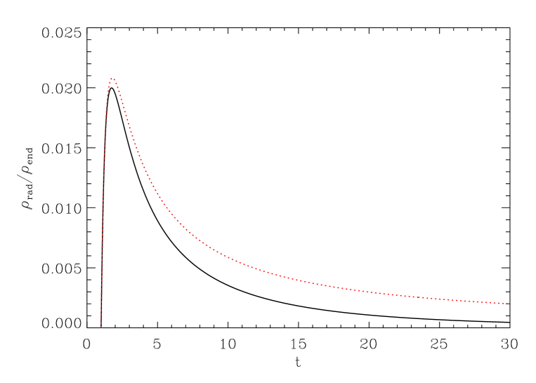
The exact (19) and approximate (20) expressions of $\rho_{\mathrm{rad}}(t)$ are presented in figure 1. At $t=t_{\mathrm{reh}}$, one can consider that the phase of reheating has been completed. After thermalisation, the energy density of radiation takes the form $\rho_{\mathrm{rad}}=g_{*}\pi^{2}T^{4}/30$ where $g_{*}$ is the number of relativistic degrees of freedom. Expressed at $t=t_{\mathrm{reh}}$, this quantity must be equal to $\rho_{\mathrm{rad}}$ in equation (20) and one arrives at

$$g_{*}^{1/4}T_{\mathrm{reh}}\simeq\left[\frac{30}{2\pi^{3}(1+w_{\mathrm{reh}})(5-3w_{\mathrm{reh}})}\right]^{1/4}\sqrt{\Gamma m_{\scriptscriptstyle{\mathrm{Pl}}}}\,,$$ (21)

where we have used $\rho_{\mathrm{end}}=3H_{\mathrm{end}}^{2}m_{\scriptscriptstyle{\mathrm{Pl}}}^{2}/(8\pi)$ and $t_{\mathrm{end}}=2H_{\mathrm{end}}^{-1}/[3(1+w_{\mathrm{reh}})]$. Moreover, The number of e-foldings during reheating can be evaluated as

$$N_{\mathrm{reh}}\simeq\frac{2}{3+3w_{\mathrm{reh}}}\ln\left(\frac{3+3w_{\mathrm{reh}}}{2}\frac{H_{\mathrm{end}}}{\Gamma}\right).$$ (22)

This result is important because it allows us to relate the physical scales now to the physical scales during inflation. To do so, one must take into account the fact that a large number of e-folds can exist during reheating. This also means that the link between what happens during inflation to what happens now depends on the details of the reheating period. In our simplified model, this period is described by a single parameter $\Gamma$ or, equivalently, $N_{\mathrm{reh}}$. One can also combine the two above equations in order to express the reheating temperature only in terms of $N_{\mathrm{reh}}$ and $w_{\mathrm{reh}}$. This leads to

$$g_{*}^{1/4}T_{\mathrm{reh}}\simeq\frac{30^{1/4}}{\sqrt{\pi}}\rho_{\mathrm{end}}^{1/4}\left(\frac{3+3w_{\mathrm{reh}}}{5-3w_{\mathrm{reh}}}\right)^{1/4}{\mathrm{e}}^{-3(1+w_{\mathrm{reh}})N_{\mathrm{reh}}/4}.$$ (23)

This expression also depends on $\rho_{\mathrm{end}}$ but this quantity is known once the background inflationary evolution is solved.

2.2 The cosmological perturbations

Having integrated the background, we now turn to the cosmological perturbations themselves. The power spectrum can be obtained by a mode by mode integration. Before addressing this issue, let us recall some basic definitions. The perturbed line element around a spatially flat FLRW universe can be expressed as [33, 34]:

$$\mathrm{d}s^{2} = a^{2}(\eta)\left\{-\left(1-2\phi\right)\mathrm{d}\eta^{2}+2\partial_{i}B\mathrm{d}x^{i}\mathrm{d}\eta+\left[\left(1-2\psi\right)\delta_{ij}\right.\right.$$ (24)

$$+ \left.\left.2\partial_{i}\partial_{j}E+h_{ij}\right]\mathrm{d}x^{i}\mathrm{d}x^{j}\right\}.$$

The four functions $\phi$, $B$, $\psi$ and $E$ represent the scalar sector whereas the transverse and traceless tensor $h_{ij}$, i.e. satisfying $h_{i}{}^{i}=\partial^{j}h_{ij}=0$, represents the gravitational waves. There are no vector perturbations because a single scalar field cannot seed curly perturbations. At the linear level, the two types of perturbations decouple and therefore can be treated separately. Since the scalar sector suffers from a gauge dependence, it is more convenient to work with the gauge-invariant Bardeen potentials $\Phi$ and the gauge-invariant perturbed scalar field $\delta\phi^{\mathrm{(gi)}}$ defined by [33, 34]

$$\Phi = \phi+\frac{1}{a}\left[a\left(B-E^{\prime}\right)\right]^{\prime}\,,\qquad\delta\phi^{\mathrm{(gi)}}=\delta\phi+\phi^{\prime}\left(B-E^{\prime}\right).$$ (25)

In the first of the two above equations, $\phi$ denotes the perturbed time-time component of the metric element (24) and not the perturbed scalar field. In fact, it is clear that one has only one degree of freedom because $\Phi$ and $\delta\phi^{\mathrm{(gi)}}$ are related by the perturbed Einstein equations. One can therefore reduce the study of the scalar sector to the study of a single variable, namely the so-called Mukhanov-Sasaki variable defined by [35]

$$v\left(\eta,\mathbf{x}\right)\equiv a\left[\delta\phi^{\mathrm{(gi)}}+\phi^{\prime}\frac{\Phi}{\mathcal{H}}\right].$$ (26)

In order to set quantum initial conditions, it turns out to be more convenient to work with the rescaled variable $\mu_{\scriptscriptstyle{\mathrm{S}}}\equiv-\sqrt{2\kappa}v$. On the other hand, the quantity of interest in the primordial power spectrum is the comoving curvature perturbation $\zeta\left(\eta,\mathbf{x}\right)$ defined by

$$\zeta=-\frac{\mu_{\scriptscriptstyle{\mathrm{S}}}}{2a\sqrt{\epsilon_{1}}}\,.$$ (27)

Since no tensorial quantity can be used to generate an infinitesimal coordinate transformation, the tensor sector is gauge invariant and fully characterised by the quantity $\mu_{\scriptscriptstyle{\mathrm{T}}}$ related to $h_{ij}$ through the relation

$$h_{ij}=\frac{\mu_{\scriptscriptstyle{\mathrm{T}}}}{a}Q_{ij}\,.$$ (28)

The $Q_{ij}$ are the transverse and traceless eigentensors of the Laplace operator on space-like hypersurfaces.

The central result of the theory of inflationary cosmological perturbations is that the quantities $\mu_{{\scriptscriptstyle{\mathrm{S}}},{\scriptscriptstyle{\mathrm{T}}}}$ (or rather their corresponding Fourier transform) both obey the equation of motion of a parametric oscillator [35, 36, 37, 38]

$$\mu_{{\scriptscriptstyle{\mathrm{S}}},{\scriptscriptstyle{\mathrm{T}}}}^{\prime\prime}+\omega_{{\scriptscriptstyle{\mathrm{S}}},{\scriptscriptstyle{\mathrm{T}}}}^{2}(k,\eta)\mu_{{\scriptscriptstyle{\mathrm{S}}},{\scriptscriptstyle{\mathrm{T}}}}=0\,,$$ (29)

where the time variation of the frequencies only depend on the behaviour of the background and is given by

$$\omega_{\scriptscriptstyle{\mathrm{S}}}^{2}\left(k,\eta\right)=k^{2}-\frac{(a\sqrt{\epsilon_{1}})^{\prime\prime}}{a\sqrt{\epsilon_{1}}}\,,\qquad\omega_{\scriptscriptstyle{\mathrm{T}}}^{2}\left(k,\eta\right)=k^{2}-\frac{a^{\prime\prime}}{a}\,.$$ (30)

In these expressions $k$ denotes the comoving wavenumber. In order to solve the above equations, one postulates that the quantum fields are initially placed in the vacuum state when the mode $k$ is well within the Hubble radius, which amounts to assume that

$$\lim_{k/(aH)\rightarrow+\infty}\mu_{{\scriptscriptstyle{\mathrm{S}}},{\scriptscriptstyle{\mathrm{T}}}}(\eta)=\mp\frac{4\sqrt{\pi}}{m_{\scriptscriptstyle{\mathrm{Pl}}}}\frac{{\rm e}^{-ik(\eta-\eta_{\rm i})}}{\sqrt{2k}},$$ (31)

where $\eta_{\rm i}$ is the initial conformal time at the beginning of inflation. Then, a mode by mode integration of equation (29) allows the determination of $\mu_{{\scriptscriptstyle{\mathrm{S}}},{\scriptscriptstyle{\mathrm{T}}}}$ for a given $k$ at any time $\eta$.

It is then straightforward to determine the resulting power spectra. From a calculation of the two-point correlation functions, one obtains

$$k^{3}P_{\zeta}(k)=\frac{k^{3}}{8\pi^{2}}\left|\frac{\mu_{\scriptscriptstyle{\mathrm{S}}}}{a\sqrt{\epsilon_{1}}}\right|^{2},\qquad k^{3}P_{h}(k)=\frac{2k^{3}}{\pi^{2}}\left|\frac{\mu_{\scriptscriptstyle{\mathrm{T}}}}{a}\right|^{2}.$$ (32)

These are the quantities that seed the subsequent CMB anisotropies. Usually, the properties of these primordial power spectra are characterised by the spectral indices and their “running”. They are defined by the coefficients of Taylor expansions of the power spectra with respect to $\ln k$, evaluated at an arbitrary pivot scale $k_{*}$, namely

$$n_{\scriptscriptstyle{\mathrm{S}}}-1\equiv\left.\frac{\mathrm{d}\ln(k^{3}P_{\zeta})}{\mathrm{d}\ln k}\right|_{k_{*}},\qquad n_{\scriptscriptstyle{\mathrm{T}}}\equiv\left.\frac{\mathrm{d}\ln(k^{3}P_{h})}{\mathrm{d}\ln k}\right|_{k_{*}}.$$ (33)

For the runnings, one similarly has the two following expressions

$$\alpha_{\scriptscriptstyle{\mathrm{S}}}\equiv\left.\frac{\mathrm{d}^{2}\ln(k^{3}P_{\zeta})}{\mathrm{d}(\ln k)^{2}}\right|_{k_{*}},\qquad\alpha_{\scriptscriptstyle{\mathrm{T}}}\equiv\left.\frac{\mathrm{d}^{2}\ln(k^{3}P_{h})}{\mathrm{d}(\ln k)^{2}}\right|_{k_{*}},$$ (34)

and in principle, we could also define the running of the running and so on.

3 Testing the slow-roll models

3.1 Basics of slow-roll inflation

It was shown in the previous section that the knowledge of the background evolution is sufficient to calculate the time-dependent frequencies $\omega_{\scriptscriptstyle{\mathrm{S}}}\left(k,\eta\right)$ and $\omega_{\scriptscriptstyle{\mathrm{T}}}(k,\eta)$ which are the only quantities needed to integrate (possibly numerically) the equations of motion of the cosmological perturbations. The slow-roll approximation allows to perturbatively estimate $\omega_{{\scriptscriptstyle{\mathrm{S}}},{\scriptscriptstyle{\mathrm{T}}}}\left(k,\eta\right)$ and, hence, to derive approximated expression for the scalar and tensor power spectra [39, 40, 41]. Although there are several definitions of the slow-roll parameters, in this article, we choose to work with the Hubble-flow parameters $\{\epsilon_{n}\}$ defined by [42, 43]

$$\epsilon_{n+1}\equiv\frac{\mathrm{d}\ln|\epsilon_{n}|}{\mathrm{d}N}\,,\qquad n\geq 0\,,$$ (35)

where, as already mentioned, $N$ is the number of e-folds since some initial time $\eta_{\mathrm{in}}$. The above hierarchy starts from $\epsilon_{0}=H_{\mathrm{in}}/H$. With this definition, all the $\epsilon_{n}$ are typically of the same order of magnitude. One has slow-roll inflation as long as $|\epsilon_{n}|\ll 1$, for all $n>0$ while, as already mentioned, inflation takes place if $\epsilon_{1}<1$.

The physical interpretation of these parameters has been discussed in Ref. [43]. Let us briefly recall the results for $\epsilon_{1}$ and $\epsilon_{2}$. Although the $\epsilon_{n}$ parameters make no reference to the matter content of the Universe (they are only defined in terms of the expansion rate), it is nevertheless interesting, when we assume that a scalar field $\phi$ is responsible for inflation, to express them in terms of $\phi$. One obtains [43]

$$\epsilon_{1}=3\frac{\dot{\phi}^{2}/2}{\dot{\phi}^{2}/2+V(\phi)}\,,\qquad\frac{\mathrm{d}}{\mathrm{d}t}\left(\frac{\dot{\phi}^{2}}{2}\right)=H\dot{\phi}^{2}\left(\frac{\epsilon_{2}}{2}-\epsilon_{1}\right).$$ (36)

From the above expressions, one sees that $\epsilon_{1}/3$ measures the ratio of the kinetic energy to the total energy (i.e. kinetic plus potential energy). Using the link between $\epsilon_{1}$ and $\epsilon_{2}$, one has

$$\dot{\epsilon}_{1}=H\epsilon_{1}\epsilon_{2}\,.$$ (37)

Therefore, given the fact that $\epsilon_{1}$ is positive definite, $\epsilon_{2}>0$ (respectively $\epsilon_{2}<0$) represents a model where the kinetic energy itself increases (respectively decreases) with respect to the total energy. From equation (36), $\epsilon_{2}=2\epsilon_{1}$ marks the frontier between models where the kinetic energy increases ($\epsilon_{2}>2\epsilon_{1}$) and the models where it decreases ($\epsilon_{2}<2\epsilon_{1}$).

It was demonstrated in [43, 44] that the Hubble-flow parameters can be expressed in terms of the inflaton potential and its derivatives. The exact expressions read

$$V(\phi) = \frac{3H^{2}m_{\scriptscriptstyle{\mathrm{Pl}}}^{2}}{8\pi}\left(1-\frac{\epsilon_{1}}{3}\right),$$ (38)

$$\frac{\mathrm{d}V}{\mathrm{d}\phi} = -3H^{2}m_{\scriptscriptstyle{\mathrm{Pl}}}\sqrt{\frac{\epsilon_{1}}{4\pi}}\left(1-\frac{\epsilon_{1}}{3}+\frac{\epsilon_{2}}{6}\right),$$ (39)

$$\frac{\mathrm{d}^{2}V}{\mathrm{d}\phi^{2}} = 3H^{2}\left(2\epsilon_{1}-\frac{\epsilon_{2}}{2}-\frac{2}{3}\epsilon_{1}^{2}+\frac{5}{6}\epsilon_{1}\epsilon_{2}-\frac{1}{12}\epsilon_{2}^{2}-\frac{1}{6}\epsilon_{2}\epsilon_{3}\right).$$ (40)

In order to have a meaningful model, the potential should be positive and, hence, $\epsilon_{1}<3$. In fact, it is more interesting to express the slow-roll parameters in terms of the potential and its derivatives because, in practice, a model is defined by its potential. Therefore, one has to invert the above expressions. At leading order in these parameters, one obtains [44]

$$H^{2} \simeq \frac{8\pi}{3m_{\scriptscriptstyle{\mathrm{Pl}}}^{2}}V,\qquad\epsilon_{1}\simeq\frac{m_{\scriptscriptstyle{\mathrm{Pl}}}^{2}}{16\pi}\left({V^{\prime}\over V}\right)^{2},\qquad\epsilon_{2}\simeq\frac{m_{\scriptscriptstyle{\mathrm{Pl}}}^{2}}{4\pi}\left[\left({V^{\prime}\over V}\right)^{2}-{V^{\prime\prime}\over V}\right],$$ (41)

$$\epsilon_{2}\epsilon_{3} \simeq \frac{m_{\scriptscriptstyle{\mathrm{Pl}}}^{4}}{32\pi^{2}}\left[{V^{\prime\prime\prime}V^{\prime}\over V^{2}}-3{V^{\prime\prime}\over V}\left({V^{\prime}\over V}\right)^{2}+2\left({V^{\prime}\over V}\right)^{4}\right],$$ (42)

where, in the present context, a prime denotes a derivative with respect to the scalar field $\phi$. Since we have pushed the calculation up to order two in the slow-roll parameters, one may be worried about the fact that we only perform the inversion at leading order. Following [45], we can define two new slow-roll parameters

$$\epsilon_{\scriptscriptstyle{\mathrm{V}}}\equiv\frac{m_{\scriptscriptstyle{\mathrm{Pl}}}^{2}}{16\pi}\left(\frac{V^{\prime}}{V}\right)^{2},\qquad\eta_{\scriptscriptstyle{\mathrm{V}}}\equiv\frac{m_{\scriptscriptstyle{\mathrm{Pl}}}^{2}}{8\pi}\frac{V^{\prime\prime}}{V}\,.$$ (43)

At the next-to-leading order, one obtains [45]

$$\epsilon_{1}=\epsilon_{\scriptscriptstyle{\mathrm{V}}}-\frac{4}{3}\epsilon_{\scriptscriptstyle{\mathrm{V}}}^{2}+\frac{2}{3}\epsilon_{\scriptscriptstyle{\mathrm{V}}}\eta_{\scriptscriptstyle{\mathrm{V}}}+\dots\,.$$ (44)

At leading order, $\epsilon_{1}=\epsilon_{\scriptscriptstyle{\mathrm{V}}}$ and one recovers the expression (41) for the first Hubble-flow parameter. As expected, the corrections to this expression are quadratic in the slow-roll parameters. Therefore, as long as the slow-roll parameters are small, the predictions for a concrete model, i.e. the corresponding location in the $(\epsilon_{1},\epsilon_{2})$ plane, are almost unchanged and, in any case, undetectable with the current data. We will come back to this issue in the following and check this claim explicitly for large fields models. Of course, if one wishes to determine, say, the scalar spectral index at quadratic order, that is to say to include the quadratic terms in the expression of $n_{\scriptscriptstyle{\mathrm{S}}}-1$ (see below), then it would be mandatory to perform the inversion at quadratic order as well.

We now turn to the perturbative expression of the power spectra. The strategy consists in expanding the power spectra about the pivot scale $k_{*}$. The choice of this particular wavenumber is a priori arbitrary but must be chosen in a way minimising the uncertainties coming from the perturbative expansion. Therefore, a good choice is around the middle of the range of scales probed by the CMB (the size of which is about three decades). Consequently, the usual choice is $k_{*}=0.05\,\mbox{Mpc}^{-1}$. The expression of $P(k)$ reads

$$\frac{k^{3}P(k)}{k^{3}P_{0}(k_{*})}=a_{0}+a_{1}\ln\left(k\over k_{*}\right)+\frac{a_{2}}{2}\ln^{2}\left(k\over k_{*}\right)+\dots\,,$$ (45)

where

$$k^{3}P_{\zeta{{}_{0}}}(k_{*})=\frac{H^{2}}{\pi\epsilon_{1}m_{\scriptscriptstyle{\mathrm{Pl}}}^{2}}\,,\qquad k^{3}P_{h{{}_{0}}}(k_{*})=16\frac{H^{2}}{\pi m_{\scriptscriptstyle{\mathrm{Pl}}}^{2}}\,.$$ (46)

The coefficients $a_{i}$ are then determined in terms of the slow-roll parameters. These calculations are non trivial especially when one goes beyond the leading order because, in that case, the usual approximations in terms of Bessel functions are no longer valid. It is therefore necessary to use more sophisticated methods either based on the WKB approximation [46, 47, 48, 49] and/or on the Green function methods [50, 51]. The latter method has been used in several works [50, 44] to derive the coefficients $a_{i}$ and we only quote the results. For scalar perturbations, one gets

$$a_{0}^{{\scriptscriptstyle{(\mathrm{S})}}} = 1-2\left(C+1\right)\epsilon_{1}-C\epsilon_{2}+\left(2C^{2}+2C+\frac{\pi^{2}}{2}-5\right)\epsilon_{1}^{2}$$ (47)

$$+ \left(C^{2}-C+\frac{7\pi^{2}}{12}-7\right)\epsilon_{1}\epsilon_{2}+\left(\frac{1}{2}C^{2}+\frac{\pi^{2}}{8}-1\right)\epsilon_{2}^{2}$$

$$+ \left(-\frac{1}{2}C^{2}+\frac{\pi^{2}}{24}\right)\epsilon_{2}\epsilon_{3}\,,$$

$$a_{1}^{{\scriptscriptstyle{(\mathrm{S})}}} = -2\epsilon_{1}-\epsilon_{2}+2(2C+1)\epsilon_{1}^{2}+(2C-1)\epsilon_{1}\epsilon_{2}+C\epsilon_{2}^{2}-C\epsilon_{2}\epsilon_{3}\,,$$ (48)

$$a_{2}^{{\scriptscriptstyle{(\mathrm{S})}}} = 4\epsilon_{1}^{2}+2\epsilon_{1}\epsilon_{2}+\epsilon_{2}^{2}-\epsilon_{2}\epsilon_{3}\,,$$ (49)

where $C\equiv\gamma_{{\scriptscriptstyle{\mathrm{E}}}}+\ln 2-2\approx-0.7296$, $\gamma_{\scriptscriptstyle{\mathrm{E}}}$ being the Euler constant. For the gravitational waves, the coefficients $a_{i}$ read

$$a_{0}^{{\scriptscriptstyle{(\mathrm{T})}}} = 1-2\left(C+1\right)\epsilon_{1}+\left(2C^{2}+2C+\frac{\pi^{2}}{2}-5\right)\epsilon_{1}^{2}$$ (50)

$$+ \left(-C^{2}-2C+\frac{\pi^{2}}{12}-2\right)\epsilon_{1}\epsilon_{2}\,,$$

$$a_{1}^{{\scriptscriptstyle{(\mathrm{T})}}} = -2\epsilon_{1}+2(2C+1)\epsilon_{1}^{2}-2(C+1)\epsilon_{1}\epsilon_{2}\,,$$ (51)

$$a_{2}^{{\scriptscriptstyle{(\mathrm{T})}}} = 4\epsilon_{1}^{2}-2\epsilon_{1}\epsilon_{2}\,.$$ (52)

We see that each coefficients $a_{i}$ starts at order $\epsilon_{n}^{i}$. In fact, this can be proven analytically since the coefficients $a_{i+1}$ can be obtained from the coefficient $a_{i}$ by differentiation with respect to the number of e-folds. Equivalently, if one is able to determine the coefficient $a_{0}$ at order $\epsilon_{n}^{i}$, then one can derive a non-vanishing expression for the coefficients $a_{j}$ up to $j=i$. The above considerations also lead to the domain of validity of the expression (45). Clearly, one has a meaningful expansion as long as

$$\epsilon_{n}\ln\left(\frac{k}{k_{*}}\right)\ll 1\,,$$ (53)

where we have again used the fact that $a_{i}$ is of order $\epsilon_{n}^{i}$. In principle, this estimate is valid for any slow-roll parameters. Given the fact that the CMB observations probe about three decades in wavenumbers and assuming that a natural location for the pivot scale $k_{*}$ has indeed been chosen in the middle of this range, one arrives at

$$|\epsilon_{n}|\ll 0.29\,.$$ (54)

In practice, in the rest of this article, we will consider that the equation (45) remains valid as long as $|\epsilon_{n}|<0.1$.

The logarithm of the power spectra can also be Taylor expanded in terms of the logarithm of the comoving wave number:

$$\ln\frac{k^{3}P(k)}{k^{3}P_{0}(k_{*})}=b_{0}+b_{1}\ln\left(k\over k_{*}\right)+\frac{b_{2}}{2}\ln^{2}\left(k\over k_{*}\right)+\dots\,,$$ (55)

where the coefficients $b_{i}$ are given by

$$b_{0}^{{\scriptscriptstyle{(\mathrm{S})}}} = -2\left(C+1\right)\epsilon_{1}-C\epsilon_{2}+\left(-2C+\frac{\pi^{2}}{2}-7\right)\epsilon_{1}^{2}$$ (56)

$$+ \left(-C^{2}-3C+\frac{7\pi^{2}}{12}-7\right)\epsilon_{1}\epsilon_{2}+\left(\frac{\pi^{2}}{8}-1\right)\epsilon_{2}^{2}$$

$$+ \left(-\frac{1}{2}C^{2}+\frac{\pi^{2}}{24}\right)\epsilon_{2}\epsilon_{3}\,,$$

$$b_{1}^{{\scriptscriptstyle{(\mathrm{S})}}} = -2\epsilon_{1}-\epsilon_{2}-2\epsilon_{1}^{2}-(2C+3)\epsilon_{1}\epsilon_{2}-C\epsilon_{2}\epsilon_{3}\,,$$ (57)

$$b_{2}^{{\scriptscriptstyle{(\mathrm{S})}}} = -2\epsilon_{1}\epsilon_{2}-\epsilon_{2}\epsilon_{3}\,,$$ (58)

for the scalar power spectrum, while the $b_{i}$’s associated with the tensor power spectrum read

$$b_{0}^{{\scriptscriptstyle{(\mathrm{T})}}} = -2\left(C+1\right)\epsilon_{1}+\left(-2C+\frac{\pi^{2}}{2}-7\right)\epsilon_{1}^{2}$$ (59)

$$+ \left(-C^{2}-2C+\frac{\pi^{2}}{12}-2\right)\epsilon_{1}\epsilon_{2}\,,$$

$$b_{1}^{{\scriptscriptstyle{(\mathrm{T})}}} = -2\epsilon_{1}-2\epsilon_{1}^{2}-2(C+1)\epsilon_{1}\epsilon_{2}\,,$$ (60)

$$b_{2}^{{\scriptscriptstyle{(\mathrm{T})}}} = -2\epsilon_{1}\epsilon_{2}\,.$$ (61)

The interest of the coefficients $b_{i}$ is that they are directly related to observable quantities, namely to the spectral indices and the runnings. Explicitly, one has

$$n_{\scriptscriptstyle{\mathrm{S}}}-1=b_{1}^{{\scriptscriptstyle{(\mathrm{S})}}}\,,\qquad n_{\scriptscriptstyle{\mathrm{T}}}=b_{1}^{{\scriptscriptstyle{(\mathrm{T})}}}\,,\qquad\alpha_{\scriptscriptstyle{\mathrm{S}}}=b_{2}^{{\scriptscriptstyle{(\mathrm{S})}}}\,,\qquad\alpha_{\scriptscriptstyle{\mathrm{T}}}=b_{2}^{{\scriptscriptstyle{(\mathrm{T})}}}\,.$$ (62)

In particular, one sees that, at first order in a consistent slow-roll expansion, the scalar and tensor runnings vanish.

Finally, the ratio of amplitudes of scalars and tensors at the pivot reads

$$r \equiv \frac{k^{3}P_{h}}{k^{3}P_{\zeta}}=16\epsilon_{1}\left[1+C\epsilon_{2}+\left(C-\frac{\pi^{2}}{2}+5\right)\epsilon_{1}\epsilon_{2}+\left(\frac{1}{2}C^{2}-\frac{\pi^{2}}{8}+1\right)\epsilon_{2}^{2}\right.$$ (63)

$$+ \left.\left(\frac{1}{2}C^{2}-\frac{\pi^{2}}{24}\right)\epsilon_{2}\epsilon_{3}\right]\,.$$

At first order, this is nothing but the consistency condition of inflation, i.e. $r=-8n_{\scriptscriptstyle{\mathrm{T}}}$. Therefore, any upper bound on the first slow-roll parameter $\epsilon_{1}$ gives an upper bound on the contribution of gravitational waves. In fact, the ratio $r$ itself is not observable because one must take into account the evolution of the transfer function when the modes re-enter the Hubble radius. If we formulate the ratio tensor to scalar in terms of CMB multipole moments, then one obtains

$$r_{10}\equiv\frac{C_{10}^{{\scriptscriptstyle{(\mathrm{T})}}}}{C_{10}^{{\scriptscriptstyle{(\mathrm{S})}}}}=-f_{10}(h,\Omega_{{}_{\Lambda}},\cdots)n_{\scriptscriptstyle{\mathrm{T}}}\,.$$ (64)

For the concordance model, one has $f_{10}\simeq 5$ which implies that $r_{10}\simeq 10\epsilon_{1}$. We see that an upper bound on $\epsilon_{1}$ puts an upper bound on $r_{10}$. This also implies an upper bound on the energy scale of inflation. Indeed, on very large scales ($\ell\ll 20$), the multipole moments can be written as

$$C_{\ell}^{{\scriptscriptstyle{(\mathrm{S})}}}\simeq\frac{2H^{2}}{25m_{\scriptscriptstyle{\mathrm{Pl}}}^{2}\epsilon_{1}}\frac{1}{\ell(\ell+1)}\,,$$ (65)

and the measurement of the quadrupole $C_{2}$ by WMAP means that

$$\left(\frac{H}{m_{\scriptscriptstyle{\mathrm{Pl}}}}\right)^{2}=60\pi\epsilon_{1}\left(\frac{Q_{\mathrm{rms-PS}}}{T}\right)^{2},$$ (66)

where [3]

$$\frac{Q_{\mathrm{rms-PS}}}{T}\equiv\sqrt{\frac{5C_{2}}{4\pi}}\simeq 6\times 10^{-6}\,.$$ (67)

As announced, any upper bound on the first slow-roll parameter implies an upper bound on $H/m_{\scriptscriptstyle{\mathrm{Pl}}}$. In the next section, the WMAP third year data are used to constrain the slow-roll parameters and an upper limit on $r_{10}$ and $H/m_{\scriptscriptstyle{\mathrm{Pl}}}$ is derived.

3.2 WMAP data constraints on the slow-roll parameters

In this section, before turning to the specific models of inflation we are interested in, we derive the bounds that the Hubble-flow parameters have to satisfy given the third year WMAP data (WMAP3). Following [52], we used a modified version of the CAMB code [10] to compute the CMB temperature and polarisation anisotropies seeded by the slow-roll scalar and tensor primordial power spectra of equation (45). The parameter space has been sampled by using Markov Chain Monte Carlo (MCMC) methods implemented in the COSMOMC code [11] and using the likelihood estimator provided by the WMAP team [2, 4, 3, 1]. The likelihood code settings have been kept to their default values which include the pixel based analysis at large scales, a Gaussian likelihood for the beam, with diagonal covariance matrix, and point source corrections [3, 53, 6]. We have also checked the sensitivity of our results to modifications of these options and no significant deviations has been observed. The assumed cosmological model is a flat $\Lambda$CDM universe involving a minimal set of four cosmological base parameters: the number density of baryons $\Omega_{\mathrm{b}}$, of cold dark matter $\Omega_{\mathrm{dm}}$, the reionization optical depth $\tau$ and $\theta$ which measures the ratio of the sound horizon to the angular diameter distance (see Ref. [11]). Moreover, we have only considered the WMAP3 data together with the Hubble Space Telescope (HST) constraint ($H_{0}=72\pm 8\,\mathrm{km/s/Mpc}$ [54]) and a top hat prior on the age of the universe between $10\,\mathrm{Gyrs}$ and $20\,\mathrm{Gyrs}$. The convergence of the chains has been assessed by using the Gelman and Rubin R–statistics implemented in COSMOMC which is a measure of the variance of the means divided by the mean value of the variances between different chains [55, 11]. Unless otherwise specified, the iterations have been stopped once $R-1<3\%$, which corresponds to a few hundred thousand samples depending on the model explored.

As described in the previous section, the set of primordial parameters in the slow-roll approximation involves the value of the scalar power spectrum $P_{*}=k^{3}P_{\zeta{{}_{0}}}(k_{*})$ and the Hubble-flow parameters evaluated at the pivot scale $k_{*}$.

3.2.1 First order slow-roll expansion

Figure 2: Marginalised posterior probability distributions for the base $\Lambda$CDM cosmological parameters together with the cosmological constant and the Hubble parameter, obtained at first order in slow-roll expansion. The solid black lines correspond to an uniform prior choice on $\epsilon_{1}$ while the dashed blue ones to an uniform prior on $\log(\epsilon_{1})$. The dotted black lines is the mean likelihood for the former prior.

At first order in the slow-roll expansion, the relevant parameters are $\epsilon_{1}$ and $\epsilon_{2}$ while the running of the spectral index vanishes. This accounts for three primordial parameters including the amplitude of the scalar power spectrum leading to seven model parameters in total. The best fit model has $\chi^{2}=11252.2$ (for comparison, the standard power law parametrisation almost leads to the same best fit value $\chi^{2}=11252.4$).

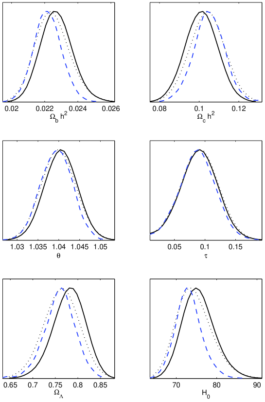
In addition to the usual uniform top hat priors on the cosmological parameters [11], we have chosen a uniform prior on $\ln(10^{10}P_{*})$ in the range $[2.7,4.0]$, as well as a uniform prior on $\epsilon_{2}$ in $[-0.2,0.2]$. As discussed in [56, 57], a prior choice on $\epsilon_{1}$ is not innocuous. This parameter encodes the amount of gravitational waves contributing to the CMB anisotropies and its order of magnitude is not known. Moreover, as shown in the next sections, even in the simplest single field inflationary models under scrutiny in this work, the orders of magnitude of $\epsilon_{1}$ may vary considerably. As a result, we have performed two MCMC analysis: one where $\epsilon_{1}$ has an uniform prior in the range $[10^{-5},10^{-1}]$ and the other with a Jeffreys’ prior by choosing an uniform prior on $\log(\epsilon_{1})$ in $[-5,0]$. We have plotted in figure 2 the marginalised posterior probability distributions for the base cosmological parameters together with $H_{0}$ and $\Omega_{\Lambda}$ for convenience. The solid and dashed line correspond to the uniform and Jeffreys’ prior on $\epsilon_{1}$, respectively.

Figure 3: $68\%$ and $95\%$ confidence intervals of the two-dimensional marginalised posteriors in the slow-roll parameters plane, obtained at leading order in slow-roll expansion. The shading is the mean likelihood and the left plot is derived under an uniform prior on $\epsilon_{1}$ while the right panel corresponds to an uniform prior on $\log(\epsilon_{1})$.

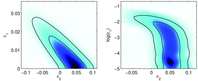
The deviations induced by the prior choice on $\epsilon_{1}$ are the consequences of the degeneracy between the two slow-roll parameters (see figure 3). As discussed in [52] this is the result of both their influence on the spectral index $n_{\scriptscriptstyle{\mathrm{S}}}=1-2\epsilon_{1}-\epsilon_{2}$ and the tensor mode contribution to the CMB anisotropies encoded in $\epsilon_{1}$. Since a Jeffreys’ prior on $\epsilon_{1}$ gives more statistical weight to its small values, the accessible volume in the parameter space is enlarged in a region where $\epsilon_{1}$ is small and the tensor modes have not observable effects. In some sense, this prior choice tends to favour pure scalar mode models. On the other hand, in the region where $\epsilon_{1}$ has a significant effect, $\epsilon_{2}$ is pushed to lower values in such a way that the scalar spectral index remains compatible with the data while the cosmological parameters react to a significant tensor mode contribution.

Figure 4: Marginalised posterior probability distributions for the primordial parameters in the first order slow-roll expansion. As in figure 2, the black solid curves are derived under an uniform prior on $\epsilon_{1}$ whereas the dashed blue curves correspond to a flat prior on $\log(\epsilon_{1})$. At two-sigma level of confidence one has the marginalised upper bound $\epsilon_{1}<0.022$.

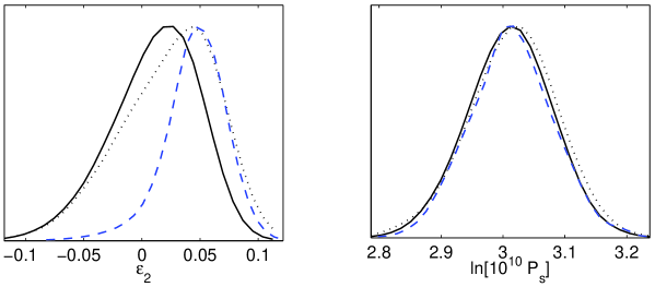
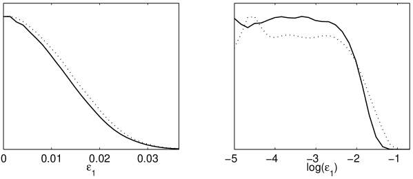
In figure 4, we have plotted the marginalised posteriors for the primordial parameters. Similarly, the probability distribution on $\epsilon_{2}$ ends up being affected by the $\epsilon_{1}$ prior choice. Since for small values of $\epsilon_{1}$ the spectral index approaches $n_{\scriptscriptstyle{\mathrm{S}}}\simeq 1-\epsilon_{2}$, under the Jeffreys’ prior on $\epsilon_{1}$ one finds the positive values of $\epsilon_{2}$ favoured: $-0.02<\epsilon_{2}<0.09$ at $2\sigma$ level while $-0.07<\epsilon_{2}<0.07$ under the uniform $\epsilon_{1}$ prior. We also obtain the marginalised upper bound $\epsilon_{1}<0.022$ at $95\%$ of confidence, or in terms of the observed tensor to scalar ratio and scale of inflation:

$$r_{10}<0.21\,,\qquad\frac{H}{m_{\scriptscriptstyle{\mathrm{Pl}}}}<1.3\times 10^{-5},$$ (68)

again at $2\sigma$.

Notice that without marginalising over $\epsilon_{2}$ one obtains slightly weaker $2\sigma$ limits $\epsilon_{1}<0.028$ and $r_{10}<0.28$. These can be compared to the unmarginalised bounds coming from the WMAP first year data and given in reference [52], namely $\epsilon_{1}<0.032$ and $r_{10}<0.32$.

3.2.2 Second order slow-roll expansion

As discussed in section 3, at second order in the slow-roll approximation, one has to consider the third Hubble-flow parameter $\epsilon_{3}$. In the following, we reiterate the previous MCMC analysis on the parameters space enlarged by $\epsilon_{3}$ under an uniform prior choice in $[-0.1,0.1]$. All the other priors have been kept as in the first order analysis, as well as the comparison between the uniform and Jeffreys’ prior on $\epsilon_{1}$. We are therefore dealing with a model involving eight parameters.

Figure 5: One and two-sigma confidence levels of the two-dimensional marginalised posteriors in the Hubble-flow parameter planes (solid black contours). The dotted red contours correspond to the same confidence intervals derived at first order in slow-roll expansion (see figure 3). The left panels are associated with an uniform prior on $\epsilon_{1}$ whereas the right ones correspond to an uniform prior on $\log(\epsilon_{1})$. As can be seen in the bottom right panel, positive values of $\epsilon_{3}$ are slightly favoured, but in a prior dependent way while $\epsilon_{3}=0$ remains within the one-sigma contour.

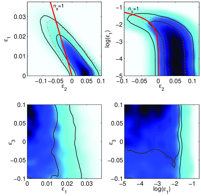
As expected for well-constrained parameters, we find no significant deviation on the base cosmological parameters and scalar power spectrum amplitude between the first and second order slow-roll models. The two-dimensional marginalised posteriors for the Hubble-flow parameters are represented in figure 5. Similarly, the one and two-sigma confidence intervals in the plane $(\epsilon_{1},\epsilon_{2})$ are found to be slightly enlarged compared to their first order equivalents, but not more than what one may expect from the inclusion of a new parameter.

Figure 6: Marginalised posterior probability distributions for the Hubble-flow parameters up to second order in the slow-roll expansion. The solid thick black curves corresponds to a uniform prior on $\epsilon_{1}$ whereas the solid thin blue curves are derived under an uniform prior on $\log(\epsilon_{1})$. The dashed curves are the corresponding first order slow-roll posteriors of figure 4.

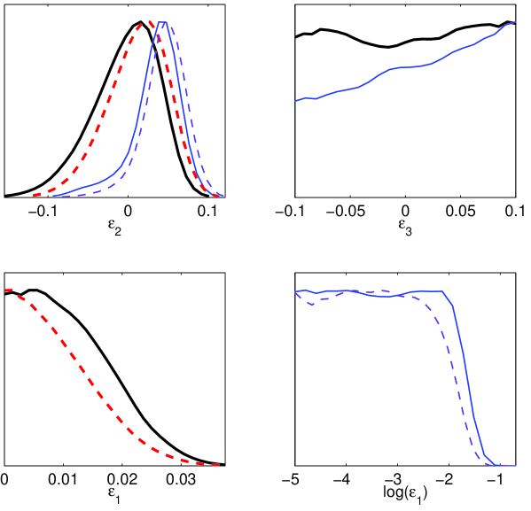
The marginalised posteriors associated with the Hubble-flow parameters are plotted in Fig. 6. Apart slightly weaker constraints on $\epsilon_{1}$ and $\epsilon_{2}$, one may notice a weak, but non-significant, tendency of running associated with positive values of $\epsilon_{3}$. However, this effect appears only when a Jeffrey’s prior is chosen on $\epsilon_{1}$ and disappears under the uniform prior choice [52, 7, 58].

3.3 Large field models

Large fields models (or chaotic inflation models although this is not very appropriate [59]) are characterised by the monomial potential given by [60]

$$V(\phi)=M^{4}\left(\frac{\phi}{m_{\scriptscriptstyle{\mathrm{Pl}}}}\right)^{p}.$$ (69)

There are only two free parameters, $M$ and $p$ and the energy scale $M$ is uniquely determined by the amplitude of the CMB anisotropies, and thus the WMAP normalisation. This is probably the simplest inflationary scenario since, in the slow-roll approximation, everything can be integrated analytically. This family of potentials is represented in figure 7.

Figure 7: Top left panel: large field potential for $p=2$ (solid green line), $p=4$ (dotted blue line) and $p=6$ (dashed red line). Top right panel: logarithm of the potentials for the same values of $p$ (and the same line style code). The required flatness of the potential becomes obvious on this plot. Bottom left panel: slow-roll parameter $\epsilon_{1}$ for a large field potential with $p=2$. The shaded area indicates the breakdown of the slow-roll inflation (strictly speaking when the acceleration stops). Bottom right panel: slow-roll parameters $\epsilon_{2}$ and $\epsilon_{3}$ for a large field potential with $p=2$. Only one curve appears because $\epsilon_{2}=\epsilon_{3}$. On this plot, the shaded region signals the breakdown of the slow-roll approximation but not necessarily the end of the accelerated phase.

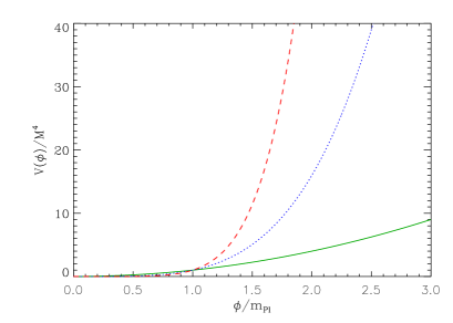
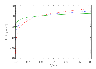
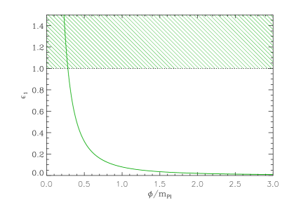
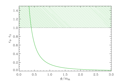
From the expression of the potential, the three slow-roll parameters can be easily computed and reads

$$\epsilon_{1}=\frac{p^{2}}{16\pi}\frac{m_{\scriptscriptstyle{\mathrm{Pl}}}^{2}}{\phi^{2}}\,,\qquad\epsilon_{2}=\frac{p}{4\pi}\frac{m_{\scriptscriptstyle{\mathrm{Pl}}}^{2}}{\phi^{2}}\,,\qquad\epsilon_{3}=\epsilon_{2}\,.$$ (70)

These slow roll parameters are represented in the two bottom panels in figure 7. There are monotonic functions of $\phi$ and they are decreasing as $\phi$ is increasing. One can immediately deduce that, for a given $p$, the model in the plane $(\epsilon_{1},\epsilon_{2})$ is represented by the trajectory $\epsilon_{1}=(p/4)\epsilon_{2}$. We can also estimate the value of the inflaton at the end of inflation, defined to be the time at which $\epsilon_{1}=1$ (see before). This leads to

$$\frac{\phi_{\mathrm{end}}}{m_{\scriptscriptstyle{\mathrm{Pl}}}}=\frac{p}{4\sqrt{\pi}}\,.$$ (71)

Moreover, the slow-roll equation of motion leads to a solution which is completely explicit. Integrating the following quadrature

$$N=-\frac{8\pi}{m_{\scriptscriptstyle{\mathrm{Pl}}}^{2}}\int_{\phi_{\mathrm{in}}}^{\phi}\frac{V(\chi)}{V^{\prime}(\chi)}\mathrm{d}\chi=-\frac{8\pi}{p}\int_{\phi_{\mathrm{in}}/m_{\scriptscriptstyle{\mathrm{Pl}}}}^{\phi/m_{\scriptscriptstyle{\mathrm{Pl}}}}x\mathrm{d}x\,,$$ (72)

leads to an explicit expression $N=N(\phi)$ which can be inverted and reads

$$\frac{\phi}{m_{\scriptscriptstyle{\mathrm{Pl}}}}=\sqrt{\left(\frac{\phi_{\mathrm{in}}}{m_{\scriptscriptstyle{\mathrm{Pl}}}}\right)^{2}-\frac{p}{4\pi}N}\,.$$ (73)

This expression also allows us to obtain the total number of e-folds. It is sufficient to evaluate the above expression for $\phi=\phi_{\mathrm{end}}$, $\phi_{\mathrm{end}}$ being given by (71). One arrives at

$$N_{\scriptscriptstyle{\mathrm{T}}}=\frac{4\pi}{p}\left(\frac{\phi_{\mathrm{in}}}{m_{\scriptscriptstyle{\mathrm{Pl}}}}\right)^{2}-\frac{p}{4}\,,$$ (74)

which can be very large if the initial energy density of the inflaton field is close to the Planck scale $m_{\scriptscriptstyle{\mathrm{Pl}}}^{4}$. However, the model remains under control only if the initial energy density is smaller than $m_{\scriptscriptstyle{\mathrm{Pl}}}^{4}$ and this imposes a constraint on the initial value of the field, namely

$$\frac{\phi_{\mathrm{in}}}{m_{\scriptscriptstyle{\mathrm{Pl}}}}\lesssim\left(\frac{m_{\scriptscriptstyle{\mathrm{Pl}}}}{M}\right)^{4/p}.$$ (75)

Let us notice that, when the inflaton energy density approaches the Planck energy density, quantum effects become important. In this case, the formalism of stochastic inflation must be used [61, 62, 63, 64, 65, 66, 67, 68]

We now turn to the explicit determination of the slow-roll parameters. We have seen that the model is represented by the trajectory $\epsilon_{1}=(p/4)\epsilon_{2}$ but observable models only lie in a limited portion of this straight line. Indeed, the Hubble-flow parameters should be evaluated when the scales of astrophysical interest today left the Hubble radius during inflation. Let us call the value of the inflaton at that time $\phi_{*}$. Then $\phi_{*}$ can be expressed in terms of $N_{*}$, the number of e-folds between the time of Hubble exit and the end of inflation:

$$N_{*}=-\frac{8\pi}{p}\int_{\phi_{*}/m_{\scriptscriptstyle{\mathrm{Pl}}}}^{\phi_{\mathrm{end}}/m_{\scriptscriptstyle{\mathrm{Pl}}}}x\mathrm{d}x\,,$$ (76)

from which one deduces

$$\frac{\phi_{*}^{2}}{m_{\scriptscriptstyle{\mathrm{Pl}}}^{2}}=\frac{p}{4\pi}\left(N_{*}+\frac{p}{4}\right).$$ (77)

Therefore, the slow roll parameters can be expressed as

$$\epsilon_{1}=\frac{p}{4\left(N_{*}+p/4\right)}\,,\qquad\epsilon_{2}=\frac{1}{N_{*}+p/4}\,,\qquad\epsilon_{3}=\epsilon_{2}\,.$$ (78)

The number of e-folds $N_{*}$ between the end of inflation and the Hubble length exit can be thought as the arc length along the straight line representing the large field models. The value of $N_{*}$ can be calculated once one knows the entire history of the Universe, including the reheating phase [69]. In the following, we will consider that

$$40<N_{*}<60\,,$$ (79)

when dealing with the slow-roll models and in fact, as explained in [69], one could consider an even more restricted range for the quartic model $p=4$.

The slow-roll predictions for the large field models are represented in figure 8.

Figure 8: Slow-roll predictions for large field models in the plane $(\epsilon_{1},\epsilon_{2})$. The dotted black lines indicate the lines of constant spectral indices from $n_{\scriptscriptstyle{\mathrm{S}}}=0.8$ (on the right) to $n_{\scriptscriptstyle{\mathrm{S}}}=1.1$ (on the left), the red line corresponding to a scale invariant spectrum $n_{\scriptscriptstyle{\mathrm{S}}}=1$. The solid blue lines separate the regions $\epsilon_{2}<0$, $\epsilon_{2}>0$, $\epsilon_{2}<2\epsilon_{1}$ and $\epsilon_{2}>2\epsilon_{1}$ associated with different energetic evolutions (see text). As expected, large field models lie in the region $\epsilon_{2}<2\epsilon_{1}$. The dotted-dashed blue curves indicate the $1\sigma$ and $2\sigma$ confidence intervals given the WMAP3 data (see section 3.2). Each coloured segment represents the prediction of a model given $p$ (see colour bar) and for a number of e-folds $N_{*}$ between the end of inflation and the Hubble exit varying in $[40,60]$.

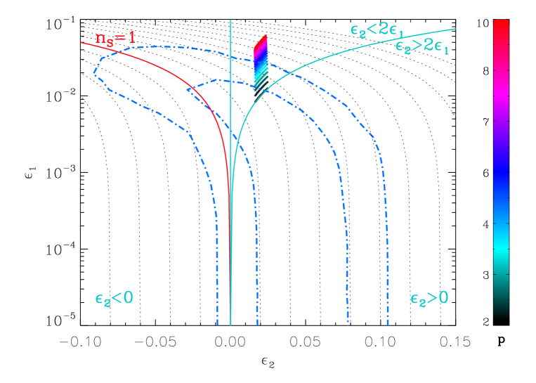
As expected, the whole family lies in the region $\epsilon_{2}>0$ and $\epsilon_{2}<2\epsilon_{1}$. According to the previous discussion, this means that, as inflation proceeds, the kinetic energy increases with respect to the total energy density and, at the same time, the absolute value of this kinetic energy density decreases. From figure 8, all the models with $p\gtrsim 4$ lie outside the $2\sigma$ contour. The quadratic (or massive) model remains compatible with the data and predicts quite a high contribution of gravitational waves, up to $r_{10}\sim 10\%$ level. Having found the compatible values of the parameter $p$, our next move is to estimate the numerical value of the parameter $M$. This can be done from the measurement of the CMB quadrupole (67) made by the WMAP satellite

$$\frac{Q_{\mathrm{rms-PS}}^{2}}{T^{2}}=\frac{1}{60\pi\epsilon_{*}}\frac{H_{*}^{2}}{m_{\scriptscriptstyle{\mathrm{Pl}}}^{2}}=\frac{2}{45\epsilon_{*}}\frac{V_{*}}{m_{\scriptscriptstyle{\mathrm{Pl}}}^{4}}\,.$$ (80)

In the case of large fields model, this implies

$$\left(\frac{M}{m_{\scriptscriptstyle{\mathrm{Pl}}}}\right)^{4}=\frac{(45/2)p}{\left(4N_{*}+p\right)^{p/2+1}}\left(\frac{16\pi}{p}\right)^{p/2}\frac{Q_{\mathrm{rms-PS}}^{2}}{T^{2}}\,,$$ (81)

and given the constraints on $p$ and $N_{*}$, this leads to

$$4\times 10^{-4}\lesssim\frac{M}{m_{\scriptscriptstyle{\mathrm{Pl}}}}\lesssim 1.1\times 10^{-3}.$$ (82)

We recover the conclusion that, for large field models, inflation take place close to the Grand Unified Theory (GUT) scale.

To conclude this section, let us come back to the question raised after equation (42), namely the error caused by expressing the slow-roll parameters $\epsilon_{n}$ in terms of the potential $V$ and its derivatives. If we take into account the more accurate equation (44), then the expression of the parameter $\epsilon_{1}$ for the quadratic model becomes

$$\epsilon_{1}=\frac{1}{4\pi}\frac{m_{\scriptscriptstyle{\mathrm{Pl}}}^{2}}{\phi^{2}}\left(1-\frac{1}{6\pi}\frac{m_{\scriptscriptstyle{\mathrm{Pl}}}^{2}}{\phi^{2}}+\dots\right).$$ (83)

From this expression, if one tries to calculate a new value of $\phi_{\mathrm{end}}$, one immediately faces the problem that the above expression leads to a second order algebraic equation with a negative discriminant, i.e. an equation which does not admit real solutions. This is not surprising since, near the end of inflation, the correction is a priori of order one. In order to have an order of magnitude estimate of the corrections, one can still work with the former value of $\phi_{\mathrm{end}}$ in (71). Then, as expected, one finds that the correction is of order $1/N_{*}^{2}\simeq 4\times 10^{-3}$ and, hence, does not in any way modify the conclusions established before about the compatibility of the large field models with the WMAP data.

3.4 Small field models

We now turn to another class of models, namely small field models. In this case, the inflaton potential can be written as [70, 71, 72]

$$V(\phi)=M^{4}\left[1-\left(\frac{\phi}{\mu}\right)^{p}\right].$$ (84)

The potential is characterised by three parameters, the energy scale $M$, $\mu$ and the index $p$, i.e. one more parameter with respect to the large field models.

Figure 9: Top left panel: small field potentials for $p=2$ (solid green line), $p=4$ (dotted blue line) and $p=6$ (dashed red line). Top right panel: logarithm of the same potentials than in the top left panel. Bottom left panel: slow-roll parameter $\epsilon_{1}$ for the model $p=2$ with $\mu/m_{\scriptscriptstyle{\mathrm{Pl}}}=0.1$ (solid line), $\mu/m_{\scriptscriptstyle{\mathrm{Pl}}}=0.5$ (dotted line) and $\mu/m_{\scriptscriptstyle{\mathrm{Pl}}}=1$ (dashed line). The dashed area indicates where the slow-roll breaks down. Bottom right panel: slow-roll parameters $\epsilon_{2}$ (solid line) and $\epsilon_{3}$ (dotted line) for $\mu/m_{\scriptscriptstyle{\mathrm{Pl}}}=1$. Note that the slow-roll parameter $\epsilon_{2}$ is non-vanishing in the limit $\phi/\mu\rightarrow 0$ where its value reads $(m_{\scriptscriptstyle{\mathrm{Pl}}}/\mu)^{2}p/(4\pi)$.

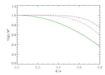
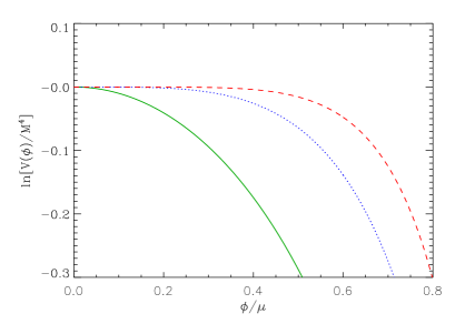
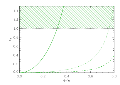
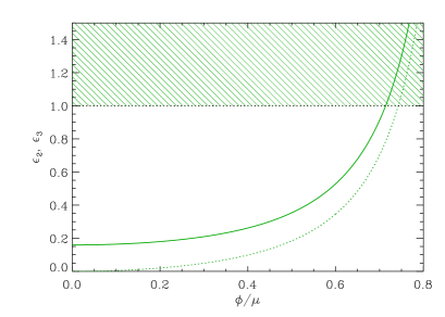
The potential, as well as its logarithm, are represented in figure 9. For these models, it is straightforward to calculate the first three slow-roll parameters. They read

$$\epsilon_{1} = \frac{p^{2}}{16\pi}\left(\frac{m_{\scriptscriptstyle{\mathrm{Pl}}}}{\mu}\right)^{2}\frac{(\phi/\mu)^{2p-2}}{\left[1-(\phi/\mu)^{p}\right]^{2}}\,,$$ (85)

$$\epsilon_{2} = \frac{p}{4\pi}\left(\frac{m_{\scriptscriptstyle{\mathrm{Pl}}}}{\mu}\right)^{2}\left(\frac{\phi}{\mu}\right)^{p-2}\frac{(\phi/\mu)^{p}+p-1}{\left[1-(\phi/\mu)^{p}\right]^{2}}\,,$$ (86)

$$\epsilon_{3} = \frac{p}{8\pi}\left(\frac{m_{\scriptscriptstyle{\mathrm{Pl}}}}{\mu}\right)^{2}\frac{\left(\phi/\mu\right)^{p-2}}{\left[1-\left(\phi/\mu\right)^{p}\right]^{2}\left[\left(\phi/\mu\right)^{p}+p-1\right]}\left[2\left(\frac{\phi}{\mu}\right)^{2p}\right.$$ (87)

$$+ \left.(p-1)(p+4)\left(\frac{\phi}{\mu}\right)^{p}+(p-1)(p-2)\right],$$

and they are represented in the two bottom panels of figure 9. As for large field models, they are monotonic functions of the field. However, these parameters are now increasing as the vacuum expectation value (vev) of the inflaton is increasing during small field inflation.

Then, we follow the same steps as in the previous subsection. Our first goal is therefore to determine when inflation stops. Requiring $\epsilon_{1}(\phi_{\mathrm{end}})=1$ leads to an algebraic equation, namely

$$\left(\frac{\phi_{\mathrm{end}}}{\mu}\right)^{2p}-2\left(\frac{\phi_{\mathrm{end}}}{\mu}\right)^{p}-\frac{p^{2}}{16\pi}\left(\frac{m_{\scriptscriptstyle{\mathrm{Pl}}}}{\mu}\right)^{2}\left(\frac{\phi_{\mathrm{end}}}{\mu}\right)^{2p-2}+1=0\,.$$ (88)

This equation can be solved explicitly for $p=2$ and the solution reads

$$\frac{\phi_{\mathrm{end}}}{\mu}=\frac{1}{4\sqrt{\pi}}\frac{m_{\scriptscriptstyle{\mathrm{Pl}}}}{\mu}\left(-1+\sqrt{1+\frac{16\pi\mu^{2}}{m_{\scriptscriptstyle{\mathrm{Pl}}}^{2}}}\right)\,.$$ (89)

In fact, among the two solutions (88) admits, we have chosen the one with the minus sign. This is because, since the vev of the inflaton field is increasing as inflation proceeds, the accelerated phase stops for the “smallest” value of $\phi_{\mathrm{end}}$. Let us notice that, in the limit, $\mu/m_{\scriptscriptstyle{\mathrm{Pl}}}\rightarrow+\infty$ one has $\phi_{\mathrm{end}}\rightarrow\mu$ but we always have $\phi_{\mathrm{end}}<\mu$, in other words the limit is approached by lower values. On the other hand, if we now assume $\mu/m_{\scriptscriptstyle{\mathrm{Pl}}}\ll 1$, then the previous solution can be approximated by

$$\frac{\phi_{\mathrm{end}}}{\mu}\simeq 2\sqrt{\pi}\frac{\mu}{m_{\scriptscriptstyle{\mathrm{Pl}}}}\,,$$ (90)

and, therefore, under the assumption $\mu/m_{\scriptscriptstyle{\mathrm{Pl}}}\ll 1$ one has $\phi_{\mathrm{end}}/\mu\ll 1$.

The above considerations were established for the case $p=2$. If $p\neq 2$ then, as already mentioned, equation (88) can no longer be explicitly solved but we can still approximate its solutions in the limits considered before. Indeed, for $\mu/m_{\scriptscriptstyle{\mathrm{Pl}}}\gg 1$, equation (88) reduces to $y^{2}-2y+1=0$, where $y=(\phi_{\mathrm{end}}/\mu)^{p}$, the only solution of which is $\phi_{\mathrm{end}}=\mu$. Consequently, as in the case $p=2$, $\phi_{\mathrm{end}}\rightarrow\mu$ when $\mu/m_{\scriptscriptstyle{\mathrm{Pl}}}\rightarrow+\infty$. On the other hand, since we always require $\phi_{\mathrm{end}}/\mu<1$, the two terms $\left(\phi_{\mathrm{end}}/\mu\right)^{2p}$ and $\left(\phi_{\mathrm{end}}/\mu\right)^{p}$ in (88) can be neglected in comparison to $1$, provided $\mu/m_{\scriptscriptstyle{\mathrm{Pl}}}\ll 1$. Then, keeping the third term on the left-hand side leads to

$$\frac{\phi_{\mathrm{end}}}{\mu}\simeq\left[\frac{16\pi}{p^{2}}\left(\frac{\mu}{m_{\scriptscriptstyle{\mathrm{Pl}}}}\right)^{2}\right]^{1/(2p-2)},$$ (91)

and one can check that, for $p=2$, this reproduces equation (90). If, on the contrary, one does not have $\mu/m_{\scriptscriptstyle{\mathrm{Pl}}}\ll 1$ (or $\mu/m_{\scriptscriptstyle{\mathrm{Pl}}}\gg 1$), then equation (88) can only be solved numerically.

The next step is to obtain the classical field trajectory for these models. This can be done if the slow-roll approximation is satisfied but, even in this case, the classical trajectory can only be found implicitly. In terms of total number of e-folds $N$, we have for the small field potential (84)

$$N=\frac{8\pi}{p}\frac{\mu^{2}}{m_{\scriptscriptstyle{\mathrm{Pl}}}^{2}}\int_{\phi_{\mathrm{in}}/\mu}^{\phi/\mu}x^{1-p}\left(1-x^{p}\right)\mathrm{d}x\,.$$ (92)

giving

$$N=\frac{4\pi}{p}\frac{\mu^{2}}{m_{\scriptscriptstyle{\mathrm{Pl}}}^{2}}\,\left\{\left(\frac{\phi_{\mathrm{in}}}{\mu}\right)^{2}-\left(\frac{\phi}{\mu}\right)^{2}+\frac{2}{p-2}\left[\left(\frac{\phi_{\mathrm{in}}}{\mu}\right)^{2-p}-\left(\frac{\phi}{\mu}\right)^{2-p}\right]\right\},$$ (93)

for $p\neq 2$, while for $p=2$ one has

$$N=2\pi\frac{\mu^{2}}{m_{\scriptscriptstyle{\mathrm{Pl}}}^{2}}\left[\left(\frac{\phi_{\mathrm{in}}}{\mu}\right)^{2}-\left(\frac{\phi}{\mu}\right)^{2}+2\ln\left(\frac{\phi}{\phi_{\mathrm{in}}}\right)\right].$$ (94)

For $p=2$, one can invert the above relation and express $\phi$ in terms of the number of e-folds to get

$$\frac{\phi}{\mu}=\sqrt{-W_{0}\left\{-\left(\frac{\phi_{\mathrm{in}}}{\mu}\right)^{2}\exp\left[-\left(\frac{\phi_{\mathrm{in}}}{\mu}\right)^{2}+\frac{N}{2\pi}\left(\frac{m_{\scriptscriptstyle{\mathrm{Pl}}}}{\mu}\right)^{2}\right]\right\}}\,,$$ (95)

where $W_{0}(x)$ is the principal branch of the Lambert function [74]. This special function is the solution of the equation

$$W(x)\rme^{W(x)}=x\,.$$ (96)

In our case, we have to choose the principal branch since $\phi/\mu<1$.

Finally, the last step consists in determining the link between $N_{*}$ and $\phi_{*}$. For $p\neq 2$, using the classical trajectory obtained before, one has to solve the following equation

$$\left(\frac{\phi_{*}}{\mu}\right)^{2}+\frac{2}{p-2}\left(\frac{\phi_{*}}{\mu}\right)^{2-p} = \frac{pN_{*}}{4\pi}\left(\frac{m_{\scriptscriptstyle{\mathrm{Pl}}}}{\mu}\right)^{2}+\left(\frac{\phi_{\mathrm{end}}}{\mu}\right)^{2}$$ (97)

$$+\frac{2}{p-2}\left(\frac{\phi_{\mathrm{end}}}{\mu}\right)^{2-p}\,,$$

where $\phi_{\mathrm{end}}$ and $N_{*}$ are known from the previous discussion.

For $p=2$, this equation can be explicitly solved and one gets

$$\frac{\phi_{*}}{\mu}=\sqrt{-W_{0}\left\{-\left(\frac{\phi_{\mathrm{end}}}{\mu}\right)^{2}\exp\left[-\left(\frac{\phi_{\mathrm{end}}}{\mu^{2}}\right)^{2}-\frac{N_{*}}{2\pi}\left(\frac{m_{\scriptscriptstyle{\mathrm{Pl}}}}{\mu}\right)^{2}\right]\right\}}\,,$$ (98)

In the limit $\mu/m_{\scriptscriptstyle{\mathrm{Pl}}}\ll 1$, the argument of the Lambert function is small and $W_{0}(x)\simeq x$ leading to

$$\left(\frac{\phi_{*}}{\mu}\right)^{2}\simeq\left(\frac{\phi_{\mathrm{end}}}{\mu}\right)^{2}\exp\left[-\left(\frac{\phi_{\mathrm{end}}}{\mu}\right)^{2}-\frac{N_{*}}{2\pi}\left(\frac{m_{\scriptscriptstyle{\mathrm{Pl}}}}{\mu}\right)^{2}\right].$$ (99)

On the other hand, in the limit $\mu/m_{\scriptscriptstyle{\mathrm{Pl}}}\rightarrow+\infty$ then, as established before, $\phi_{\mathrm{end}}\rightarrow\mu$ and the argument of the Lambert function goes to $-1/e$. Since $W_{0}(-1/e)=-1$, one obtains $\phi_{*}\rightarrow\mu$.

If $p\neq 2$, then equation (97) cannot be solved explicitly. However, in the limit $\mu/m_{\scriptscriptstyle{\mathrm{Pl}}}\ll 1$, one has $\phi_{*}\ll\mu$ and $\phi_{\mathrm{end}}/\mu\ll 1$ allowing (97) to be approximated as

$$\frac{2}{2-p}\left(\frac{\phi_{*}}{\mu}\right)^{2-p}\simeq\frac{pN_{*}}{4\pi}\left(\frac{m_{\scriptscriptstyle{\mathrm{Pl}}}}{\mu}\right)^{2}+\frac{2}{2-p}\left(\frac{\phi_{\mathrm{end}}}{\mu}\right)^{2-p}.$$ (100)

Using the expression of $\phi_{\mathrm{end}}$ obtained in (91) renders the second term in the right-hand side of the previous equation proportional to $(m_{\scriptscriptstyle{\mathrm{Pl}}}/\mu)^{(p-2)/(p-1)}$. Under the considered limit $\mu/m_{\scriptscriptstyle{\mathrm{Pl}}}\ll 1$, this term can be neglected in comparison to the the first one which is proportional to $(m_{\scriptscriptstyle{\mathrm{Pl}}}/\mu)^{2}$. Putting everything together, one gets

$$\frac{\phi_{*}}{\mu}\simeq\left[\frac{p(p-2)N_{*}}{8\pi}\left(\frac{m_{\scriptscriptstyle{\mathrm{Pl}}}}{\mu}\right)^{2}\right]^{1/(2-p)}.$$ (101)

Let us stress again that the above result is valid only for $\mu/m_{\scriptscriptstyle{\mathrm{Pl}}}\ll 1$. If this is not the case, one has to rely on numerical calculations to find the correct value of $\phi_{*}$.

The values of the slow-roll parameters directly stem from the previous considerations. If $p=2$, it is sufficient to use the value of $\phi_{*}$ found in (98) into the expressions (85) to (87). The only underlying approximation being in that case the inversion mentioned in section 2.2. Besides, assuming the limit $\mu/m_{\scriptscriptstyle{\mathrm{Pl}}}\ll 1$, one arrives at

$$\epsilon_{1} \simeq \exp\left[-\frac{N_{*}}{2\pi}\left(\frac{m_{\scriptscriptstyle{\mathrm{Pl}}}}{\mu}\right)^{2}\right],$$ (102)

$$\epsilon_{2} \simeq \frac{1}{2\pi}\left(\frac{m_{\scriptscriptstyle{\mathrm{Pl}}}}{\mu}\right)^{2},$$ (103)

$$\epsilon_{3} \simeq 6\exp\left[-\frac{N_{*}}{2\pi}\left(\frac{m_{\scriptscriptstyle{\mathrm{Pl}}}}{\mu}\right)^{2}\right].$$ (104)

These expressions coincide with the formulas already used in the literature [72, 15, 5] and it is crucial to keep in mind that they are valid for $\mu/m_{\scriptscriptstyle{\mathrm{Pl}}}\ll 1$ only.

Figure 10: Slow-roll parameters $\epsilon_{1}$ (blue lines) and $\epsilon_{2}$ (red lines) for the small field model characterised by $p=2$ and $N_{*}=40$, plotted for different values of the scale $\mu/m_{\scriptscriptstyle{\mathrm{Pl}}}$. The dotted lines are the approximations established in equations (102) to (104) whereas the solid lines are the slow-roll parameters expressed in terms of the Lambert function: the only approximation involved in that case being the inversion discussed in section 2.2.

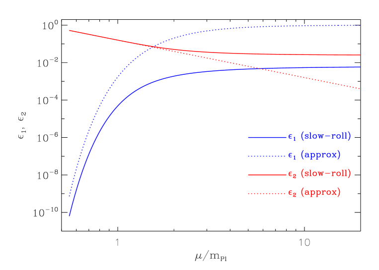
In figure 10 the slow-roll parameters $\epsilon_{1}$ and $\epsilon_{2}$ stemming from the approximate equations (102) and (103) are represented together with the ones obtained from the exact expression of $\phi_{*}$ in (98). The plot is made for $N_{*}=40$ (and $p=2$). One sees that as long as $\mu/m_{\scriptscriptstyle{\mathrm{Pl}}}\ll 1$, the two expressions of $\epsilon_{1}$ and $\epsilon_{2}$ are in good agreement but when $\mu\simeq m_{\scriptscriptstyle{\mathrm{Pl}}}$ the difference is no longer negligible. It turns out that this difference is of utmost importance in view of the current data because using only the equations (102) to (104) leads to the incorrect conclusion that the small field model $p=2$ is ruled out. In fact, using directly the slow-roll equations shows that this model is still compatible with the observations. Indeed, very roughly speaking, the WMAP3 data are compatible with $\epsilon_{1}<0.03$ and $\epsilon_{2}\simeq 0.05$. If one decides to use (103) for $\epsilon_{2}$, then $\mu\simeq 1.8m_{\scriptscriptstyle{\mathrm{Pl}}}$ and inserting back this value into (102), one finds $\epsilon_{1}\simeq 0.13$, i.e. a value in tension with the observations. The true story is quite different. As can be seen in figure 10, the slow-roll value $\epsilon_{2}\simeq 0.05$ is perfectly compatible with a value for $\epsilon_{1}$ satisfying the WMAP3 bound. The model is thus still compatible with the observational constraints. This conclusion is indeed confirmed by the exact numerical integration performed in the next section. In addition, we will demonstrate below that $\mu/m_{\scriptscriptstyle{\mathrm{Pl}}}\ll 1$ implies a very low energy scale during inflation that can be, in some cases to be discussed in the following, below the nucleosynthesis scale, i.e. already ruled out. In this situation, the small field models make sense only if $\mu\gtrsim m_{\scriptscriptstyle{\mathrm{Pl}}}$, that is to say precisely the situation where it is necessary to carefully evaluate the values of the slow-roll parameters.

Figure 11: Comparison of the slow-roll predictions for small field models with $p=3$ and $0.1<\mu/m_{\scriptscriptstyle{\mathrm{Pl}}}<20$ in the plane $(\epsilon_{1},\epsilon_{2})$. The solid red and blues lines, as well as the blue dotted-dashed contours, have the same meaning as in figure 8. The approximated slow-roll values are obtained using the equations (105) and (106) and are represented by the two red dotted vertical lines. The red dotted line on the left corresponds to models with different values of $\mu/m_{\scriptscriptstyle{\mathrm{Pl}}}$ at fixed $N_{*}=60$ while the red dotted line on the right is obtained for $N_{*}=40$. The correct slow-roll parameter values are obtained by numerical integrations and are represented by the line segments. Each line segment corresponds to a model with a fixed value of $\mu/m_{\scriptscriptstyle{\mathrm{Pl}}}$, indicated by the colour bar, along which the quantity $N_{*}$ varies from $40$ to $60$.

Let us now turn to the expressions of the slow-roll parameters in the case $p\neq 2$. If $\mu/m_{\scriptscriptstyle{\mathrm{Pl}}}\ll 1$, then one has

$$\epsilon_{1} \simeq \frac{p^{2}}{16\pi}\left(\frac{m_{\scriptscriptstyle{\mathrm{Pl}}}}{\mu}\right)^{2}\left[N_{*}\frac{p(p-2)}{8\pi}\left(\frac{m_{\scriptscriptstyle{\mathrm{Pl}}}}{\mu}\right)^{2}\right]^{-\frac{2(p-1)}{p-2}},$$ (105)

$$\epsilon_{2} \simeq \frac{2}{N_{*}}\frac{p-1}{p-2}\,,\qquad\epsilon_{3}\simeq\frac{1}{N_{*}}\,,$$ (106)

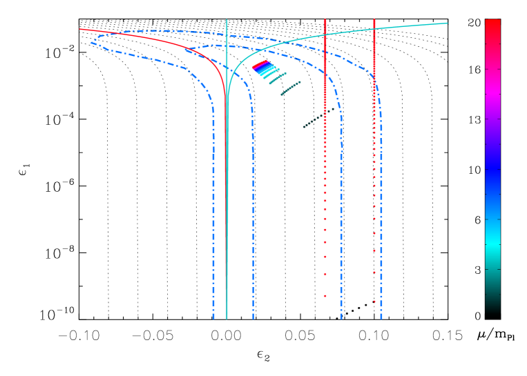
which matches to the expressions usually used in the literature. On the other hand, if the limit $\mu/m_{\scriptscriptstyle{\mathrm{Pl}}}\ll 1$ is not satisfied, the slow-roll parameters can only be estimated from numerical calculations. In figure 11, we have precisely compared the approximations given by the equations (105) and (106) to the directly computed slow-roll parameters in a model with $p=3$. The approximated values are represented by the two red dotted curves, the left one corresponding to the choice $N_{*}=60$ and the right one to $N_{*}=40$. These two curves appear as vertical lines because the expression of $\epsilon_{2}$ in (105) does not depend on $\mu/m_{\scriptscriptstyle{\mathrm{Pl}}}$. The correct values for the slow-roll parameters obtained by numerical determination of $\phi_{*}$ are represented by the line segments, $N_{*}$ varying from $40$ to $60$ along each segment. Although both methods are in good agreement for $\mu/m_{\scriptscriptstyle{\mathrm{Pl}}}\ll 1$, they differ when $\mu\gtrsim m_{\scriptscriptstyle{\mathrm{Pl}}}$. As it was the case for $p=2$, we see that using only (105) would lead us to the erroneous conclusion that the model $p=3$ is compatible with the data only if $\mu/m_{\scriptscriptstyle{\mathrm{Pl}}}\ll 1$. On the contrary, the correct values of the slow-roll parameters indicate that models with $\mu\gtrsim m_{\scriptscriptstyle{\mathrm{Pl}}}$ are simply in perfect agreement with WMAP3 data. Therefore, given the accuracy of the current CMB data, it becomes mandatory to carefully estimate the slow-roll parameters in the case of small field models. This will be confirmed by the full numerical integration of the power spectrum performed in the next section.

Figure 12: Small field models in the plane $(\epsilon_{1},\epsilon_{2})$ for $0.2<\mu/m_{\scriptscriptstyle{\mathrm{Pl}}}<20$, $p=2$ (top left panel), $p=4$ (top right panel), $p=6$ (bottom left) and $p=8$ (bottom right). The solid red and blues lines, as well as the blue dotted-dashed contours have the same meaning as in figure 8. Each curved segment represents the slow-roll predictions along which $N_{*}$ varies from $40$ to $60$.

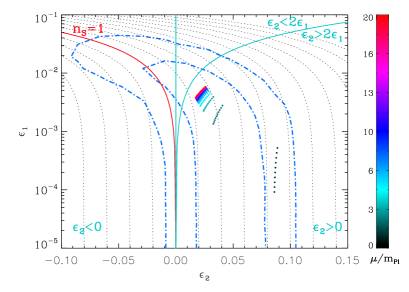
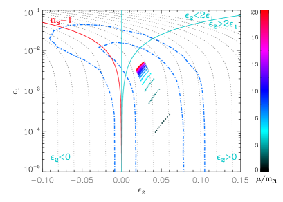
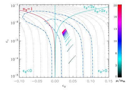
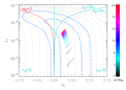
Let us now more precisely consider the predictions associated with the small field models. In figure 12, the slow-roll parameters values are represented for $0.2<\mu/m_{\scriptscriptstyle{\mathrm{Pl}}}<20$ and for four models, namely $p=2,4,6$ and $p=8$. As expected, the models are located in the region where $\epsilon_{2}>2\epsilon_{1}>0$, i.e. in the region where the kinetic energy grows with time during inflation. One can see in figure 12 that, for any value of $p$ (including $p=2$), the models are in good agreement with the data if $\mu\gtrsim m_{\scriptscriptstyle{\mathrm{Pl}}}$. This conclusion is confirmed by the full numerical integration done in the next section. In fact, only the very small values of $\mu/m_{\scriptscriptstyle{\mathrm{Pl}}}$ are problematic since they end up being associated with a too large slow-roll parameter $\epsilon_{2}$. This can be seen in the top left panel ($p=2$) where the line segments representing the $\mu/m_{\scriptscriptstyle{\mathrm{Pl}}}\lesssim 1$ models are only marginally compatible with the confidence intervals or even ruled out. In fact, in the top left panel, this is not so apparent at first sight since the models corresponding to the segment line which lies between the one and two sigma contours are still acceptable fits to the data. However, one has to realize that, for even smaller values of $\mu/m_{\scriptscriptstyle{\mathrm{Pl}}}$, the corresponding line segments are actually outside the figure, hence the above claim. Moreover, one notices that the segment line has the tendency to become vertical which indicates that the value of $\epsilon_{2}$ is independent from $N_{*}$. This is in full agreement with equation (103) giving $\epsilon_{2}$.

Finally, one word is in order on the CMB normalisation in those models and the values of $\epsilon_{1}$. It is known that the very small values of $\epsilon_{1}$ imply a very small contribution of gravitational waves. But they also imply a quite low energy scale during inflation. This allows us to derive a lower bound on $\epsilon_{1}$. Indeed, the normalisation of the spectrum is given by

$$\frac{V_{*}}{m_{\scriptscriptstyle{\mathrm{Pl}}}^{4}}\simeq\frac{45\epsilon_{1}}{2}\frac{Q_{\mathrm{rms-PS}}^{2}}{T^{2}}\,.$$ (107)

Now, it is physically motivated that inflation must take place at an energy scale at least greater than, say, the TeV scale. This means $V_{*}/m_{\scriptscriptstyle{\mathrm{Pl}}}^{4}\gtrsim 10^{-64}$ and for $p=2$ (and $N_{*}=50$), one gets $\mu\gtrsim 0.25m_{\scriptscriptstyle{\mathrm{Pl}}}$. Such a strong lower bound on $\mu$ is essentially due to the exponential behaviour of the slow-roll parameter with respect to the model parameters. In fact, this condition can equally be worked out for $p\neq 2$. For instance, with $p=2.1$ one obtains $\mu\gtrsim 0.03m_{\scriptscriptstyle{\mathrm{Pl}}}$, $p=2.5$ leads to $\mu\gtrsim 7\times 10^{-6}m_{\scriptscriptstyle{\mathrm{Pl}}}$, $p=3$ to $\mu\gtrsim 3\times 10^{-9}m_{\scriptscriptstyle{\mathrm{Pl}}}$ and $p=10$ corresponds to $\mu\gtrsim 8\times 10^{-21}m_{\scriptscriptstyle{\mathrm{Pl}}}$. These results sustain the remark made before motivating a careful determination of the slow-roll parameters in the regime $\mu\gtrsim m_{\scriptscriptstyle{\mathrm{Pl}}}$.

3.5 Hybrid inflation

Let us now turn to hybrid inflation. This case is slightly different since hybrid inflation is in fact a two-field model with the potential [75, 76, 16]

$$V\left(\phi,\psi\right)=\frac{1}{2}m^{2}\phi^{2}+\frac{\lambda^{\prime}}{4}\left(\psi^{2}-\Delta^{2}\right)^{2}+\frac{\lambda}{2}\phi^{2}\psi^{2}\,,$$ (108)

where $\phi$ is the inflaton, $\psi$ the waterfall field and $\lambda^{\prime}$ and $\lambda$ are two coupling constants. Inflation proceeds along the valley given by $\psi=0$ and, in this case, the potential reduces to an effective single field potential that can be written as

$$V(\phi)=M^{4}\left[1+\left(\frac{\phi}{\mu}\right)^{p}\right],$$ (109)

with $p=2$ and where one has used the following redefinitions

$$M=\frac{\lambda^{\prime}{}^{1/4}\Delta}{\sqrt{2}}\,,\qquad\mu=\sqrt{\frac{\lambda^{\prime}}{2}}\frac{\Delta^{2}}{m}\,.$$ (110)

As for small field models, the effective potential (109) depends on three parameters, namely $M$, $\mu$ and $p$. In fact, as mentioned before, $p=2$ for the two field model given in (108) but, to consider the most general situation we leave $p$ unspecified in the following equations. Indeed, one could consider a model where the inflationary valley is described by, say, a quartic potential since the instability mechanism is independent from the shape of the valley. Moreover, in the second part of this article, when we perform the full numerical analysis, we will consider $p$ as a free parameter and obtain its corresponding posterior probability distribution. Finally, let us emphasize that since we use a single field modelisation of hybrid inflation, such a representation cannot account for multifield effects as the generation of isocurvature modes or cosmic strings [77, 78, 17, 79]. The potential (109) and its logarithm are represented in figure 13 for different values of the power $p$.

Figure 13: Top left panel: hybrid field potential for $p=2$ (solid green line), $p=4$ (blue dotted line) and $p=6$ (red dashed line). Top right panel: logarithm of the potential for $p=2,4,6$ (same colour code as in the top left panel). Bottom left panel: slow-roll parameter $\epsilon_{1}$ for $p=2$ and $\mu/m_{\scriptscriptstyle{\mathrm{Pl}}}=0.1$ (solid line), $\mu/m_{\scriptscriptstyle{\mathrm{Pl}}}=1/(4\sqrt{\pi})\simeq 0.14$ (dotted line) and $\mu/m_{\scriptscriptstyle{\mathrm{Pl}}}=0.3$ (dashed line). Bottom right panel: slow-roll parameter $\epsilon_{2}$ (solid line) and $\epsilon_{3}$ (dotted line) both for $\mu/m_{\scriptscriptstyle{\mathrm{Pl}}}=0.3$.

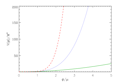
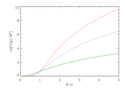
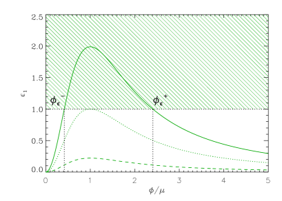
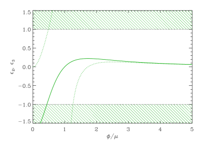
The calculation of the slow-roll parameters proceeds as usual. The explicit expressions are given by

$$\epsilon_{1} = \frac{p^{2}}{16\pi}\left(\frac{m_{\scriptscriptstyle{\mathrm{Pl}}}}{\mu}\right)^{2}\frac{(\phi/\mu)^{2p-2}}{\left[1+(\phi/\mu)^{p}\right]^{2}}\,,$$ (111)

$$\epsilon_{2} = \frac{p}{4\pi}\left(\frac{m_{\scriptscriptstyle{\mathrm{Pl}}}}{\mu}\right)^{2}\left(\frac{\phi}{\mu}\right)^{p-2}\frac{(\phi/\mu)^{p}-p+1}{\left[1+(\phi/\mu)^{p}\right]^{2}}\,,$$ (112)

$$\epsilon_{3} = \frac{p}{8\pi}\left(\frac{m_{\scriptscriptstyle{\mathrm{Pl}}}}{\mu}\right)^{2}\frac{\left(\phi/\mu\right)^{p-2}}{\left[1+\left(\phi/\mu\right)^{p}\right]^{2}\left[\left(\phi/\mu\right)^{p}-p+1\right]}\left[2\left(\frac{\phi}{\mu}\right)^{2p}\right.$$ (113)

$$- \left.(p-1)(p+4)\left(\frac{\phi}{\mu}\right)^{p}+(p-1)(p-2)\right]\,.$$

The three parameters are plotted in figure 13 in the case $p=2$. We see that the parameter $\epsilon_{1}$ has a maximum at $\phi/\mu=1$ which corresponds to the inflexion point of $\ln V$. If $\mu<1/(4\sqrt{\pi})$ then $\epsilon_{1}<1$ for all values of $\phi$. We come back to this point below when we discuss how to stop inflation. Another specific feature of hybrid inflation in comparison to large and small field models is that, as can be seen on the bottom right panel, the parameters $\epsilon_{2}$ and $\epsilon_{3}$ can be negative. In particular

$$\lim_{\phi/\mu\rightarrow 0}\epsilon_{2}=-\frac{p(p-1)}{4\pi}\left(\frac{m_{\scriptscriptstyle{\mathrm{Pl}}}}{\mu}\right)^{2}\left(\frac{\phi}{\mu}\right)^{p-2},$$ (114)

and $\epsilon_{3}$ blows up in the limit $(\phi/\mu)^{p}\rightarrow p-1$.

We now discuss how inflation ends and how to calculate $\phi_{\mathrm{end}}$. In the hybrid scenario there are a priori two mechanisms for ending inflation. Either inflation stops by instability when the inflaton reaches a value

$$\phi_{\mathrm{cri}}=\frac{\lambda^{\prime}}{\lambda}\Delta\,,$$ (115)

for which the mass in the direction perpendicular to the inflationary valley becomes negative, or the slow-roll conditions are violated and $\epsilon_{1}=1$. The latter condition happens for a field value $\phi_{\epsilon}$ solution of

$$\left(\frac{\phi_{\epsilon}}{\mu}\right)^{2p}+2\left(\frac{\phi_{\epsilon}}{\mu}\right)^{p}-\frac{p^{2}}{16\pi}\left(\frac{m_{\scriptscriptstyle{\mathrm{Pl}}}}{\mu}\right)^{2}\left(\frac{\phi_{\epsilon}}{\mu}\right)^{2p-2}+1=0\,.$$ (116)

The difference between this equation and (88) resides only in the sign of the $\left(\phi_{\epsilon}/\mu\right)^{p}$ term. This equation admits a solution only if the following condition is fulfilled: $\mu/m_{\scriptscriptstyle{\mathrm{Pl}}}<1/(4\sqrt{\pi})$. In figure 13, such situations correspond to the case where $\epsilon_{1}$ can be greater than one. If $\mu/m_{\scriptscriptstyle{\mathrm{Pl}}}>1/(4\sqrt{\pi})$ then $\epsilon_{1}$ is always smaller than one and inflation can only stop by instability. The above equation (116) cannot be solved explicitly unless $p=2$. In this case, one obtains

$$\frac{\phi_{\epsilon}}{\mu}=\frac{1}{4\sqrt{\pi}}\frac{m_{\scriptscriptstyle{\mathrm{Pl}}}}{\mu}\left(1\pm\sqrt{1-\frac{16\pi\mu^{2}}{m_{\scriptscriptstyle{\mathrm{Pl}}}^{2}}}\right).$$ (117)

Of course, one recovers the fact that the solutions exist only if $\mu/m_{\scriptscriptstyle{\mathrm{Pl}}}<1/(4\sqrt{\pi})$. The positive sign corresponds to the largest root, $\phi_{\epsilon}^{+}$, while the minus sign corresponds to the smallest one, $\phi_{\epsilon}^{-}$ (see figure 13). In the limit $\mu/m_{\scriptscriptstyle{\mathrm{Pl}}}\ll 1$ the previous equation takes the form

$$\frac{\phi_{\epsilon}}{\mu}\simeq\frac{m_{\scriptscriptstyle{\mathrm{Pl}}}}{2\mu\sqrt{\pi}}\,,$$ (118)

and one recovers the large field value of $\phi_{\mathrm{end}}$ [see for instance equation (71)]. More generally, in the limit of small $\mu/m_{\scriptscriptstyle{\mathrm{Pl}}}$, one can even approximately solve (116) for $p\neq 2$. However, contrary to the small field models case and besides the term proportional to $p^{2}$, one should keep the term $\left(\phi_{\epsilon}/\mu\right)^{2p}$ rather than $1$. This leads to

$$\frac{\phi_{\epsilon}}{\mu}\simeq\frac{pm_{\scriptscriptstyle{\mathrm{Pl}}}}{4\mu\sqrt{\pi}}\,,$$ (119)

which is the large field model expression of $\phi_{\mathrm{end}}$ for a potential with an arbitrary power $p$ in the field. Therefore, the final value $\phi_{\mathrm{end}}$ of the inflaton is the maximum of $\phi_{\mathrm{cri}}$ and $\phi_{\epsilon}$. To decide which mechanism is realised in practice requires the knowledge of the model parameters. However, one crucial interest of hybrid inflation is that inflation can proceed for small values of the inflaton vev. As we have seen before, if the inflaton vev is large, then the model is equivalent to a large field model which was already considered in a previous subsection. Therefore, in the following, we will be focused on hybrid inflation taking place for $\phi<\phi_{\epsilon}^{-}$ only: the so-called vacuum dominated regime. Since $\epsilon_{1}$ is always lower than unity in such cases (see figure 13), hybrid inflation must stop by instability. As a result, $\phi_{\mathrm{cri}}<\phi_{\epsilon}^{-}$ will be considered in the following as a free parameter accounting for a total of four inflationary parameters.

The next step consists in calculating the classical trajectory. Straightforward manipulations similar to the ones performed for small field models, lead to

$$N=\kappa^{2}\frac{\mu^{2}}{2p}\,\left\{\left(\frac{\phi_{\mathrm{in}}}{\mu}\right)^{2}-\left(\frac{\phi}{\mu}\right)^{2}-\frac{2}{p-2}\left[\left(\frac{\phi_{\mathrm{in}}}{\mu}\right)^{2-p}-\left(\frac{\phi}{\mu}\right)^{2-p}\right]\right\}\,,$$ (120)

for $p\neq 2$, where $\kappa\equiv\sqrt{8\pi}/m_{\scriptscriptstyle{\mathrm{Pl}}}$ is the reduced Planck mass. For $p=2$ one has

$$N=\kappa^{2}\frac{\mu^{2}}{4}\left[\left(\frac{\phi_{\mathrm{in}}}{\mu}\right)^{2}-\left(\frac{\phi}{\mu}\right)^{2}-2\ln\left(\frac{\phi}{\phi_{\mathrm{in}}}\right)\right],$$ (121)

which can be inverted to express $\phi$ in terms of the number of e-folds:

$$\frac{\phi}{\mu}=\sqrt{W_{0}\left\{\left(\frac{\phi_{\mathrm{in}}}{\mu}\right)^{2}\exp\left[\left(\frac{\phi_{\mathrm{in}}}{\mu}\right)^{2}-\frac{N}{2\pi}\left(\frac{m_{\scriptscriptstyle{\mathrm{Pl}}}}{\mu}\right)^{2}\right]\right\}}\,.$$ (122)

Once again, $W_{0}(x)$ denotes the principal branch of the Lambert function [74]. The above expression is very similar to equation (95), except for the signs.

As for the other models, the last step consists in determining the link between $N_{*}$ and $\phi_{*}$. For $p\neq 2$, using the classical trajectory obtained before, one has to solve the following equation

$$\left(\frac{\phi_{*}}{\mu}\right)^{2}-\frac{2}{p-2}\left(\frac{\phi_{*}}{\mu}\right)^{2-p} = \frac{pN_{*}}{4\pi}\left(\frac{m_{\scriptscriptstyle{\mathrm{Pl}}}}{\mu}\right)^{2}+\left(\frac{\phi_{\mathrm{cri}}}{\mu}\right)^{2}$$ (123)

$$- \frac{2}{p-2}\left(\frac{\phi_{\mathrm{cri}}}{\mu}\right)^{2-p},$$

where $\phi_{\mathrm{cri}}$ and $N_{*}$ are known from the previous steps. In general, this equation can only be solved numerically. However, if $p=2$, one gets

$$\frac{\phi_{*}}{\mu}=\sqrt{W_{0}\left\{\left(\frac{\phi_{\mathrm{cri}}}{\mu}\right)^{2}\exp\left[\left(\frac{\phi_{\mathrm{cri}}}{\mu}\right)^{2}+\frac{N_{*}}{2\pi}\left(\frac{m_{\scriptscriptstyle{\mathrm{Pl}}}}{\mu}\right)^{2}\right]\right\}}.$$ (124)

The slow-roll parameters for $p=2$ are then obtained by inserting the above equation into the expressions (111) to (113). We therefore have an explicit form for the three parameters $\epsilon_{1}$, $\epsilon_{2}$ and $\epsilon_{3}$ which become explicit functions of $\mu$, $\phi_{\mathrm{cri}}$ and $N_{*}$. In the so-called vacuum dominated regime we are interested in, the term $(\phi/\mu)^{2}$ in the expression of the potential (109) ends up being a small correction only. Note that in the opposite situation, i.e. the inflaton dominated regime, the model is equivalent to chaotic inflation which was already treated in the section devoted to large fields models. This question is discussed in more details below.

In Fig. 14, we have plotted the slow-roll predictions in the plane $(\epsilon_{1},\epsilon_{2})$ for different values of $\mu/m_{\scriptscriptstyle{\mathrm{Pl}}}$ and $10^{-6}<\phi_{\mathrm{cri}}/\mu<10^{-1}$. The values of $\mu/m_{\scriptscriptstyle{\mathrm{Pl}}}$ that we consider go from $\mu/m_{\scriptscriptstyle{\mathrm{Pl}}}=0.6$ (top left panel) to $\mu/m_{\scriptscriptstyle{\mathrm{Pl}}}=1.8$ (bottom right panel). Let us now discuss in more details these plots.

Figure 14: Top left panel: slow-roll predictions for hybrid inflation with $p=2$, $\mu/m_{\scriptscriptstyle{\mathrm{Pl}}}=0.6$, $10^{-6}<\phi_{\mathrm{cri}}/\mu<10^{-1}$. The colour bar indicates the value of $\log(\phi_{\mathrm{cri}}/\mu)$ and the number of e-folds $N_{*}$ is between $40$ and $60$. The other panels display different values of $\mu/m_{\scriptscriptstyle{\mathrm{Pl}}}$, the other parameters being unchanged: $\mu/m_{\scriptscriptstyle{\mathrm{Pl}}}=0.8$ (top right), $\mu/m_{\scriptscriptstyle{\mathrm{Pl}}}=1$ (middle left), $\mu/m_{\scriptscriptstyle{\mathrm{Pl}}}=1.4$ (middle right), $\mu/m_{\scriptscriptstyle{\mathrm{Pl}}}=1.6$ (bottom left) and $\mu/m_{\scriptscriptstyle{\mathrm{Pl}}}=1.8$ (bottom right). The solid red and blues lines, as well as the blue dotted-dashed contours, have the same meaning as in figure 8.

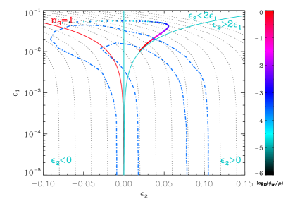
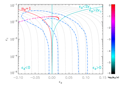
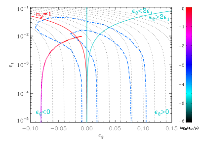
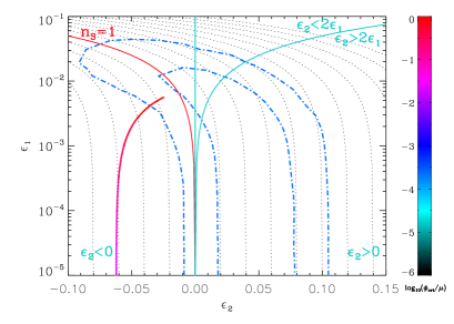
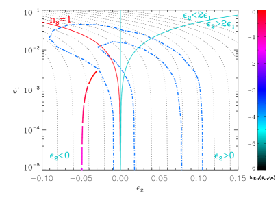
For $\mu/m_{\scriptscriptstyle{\mathrm{Pl}}}=0.6$, some models lie in the region $\epsilon_{2}>0$ and others in the region $\epsilon_{2}<0$. The first ones corresponds to $\phi_{\mathrm{cri}}/\mu$ close to the upper limit chosen for the plot, namely $10^{-1}$ while the second ones are valid for small values as one can check on the colour bar. The interpretation is as follows. When the value of $\phi_{\mathrm{cri}}$ is close to its upper bound, inflation proceeds in a regime where the term $(\phi/\mu)^{2}$ in the potential (109) is dominant. In this case, the model behaves as a quadratic large field model and this explains why the models are concentrated along the line $\epsilon_{2}=2\epsilon_{1}$. When the value of $\phi_{\mathrm{cri}}/\mu$ becomes smaller, inflation can proceeds for very small values of the inflaton vev and one enters the vacuum dominated regime which is the main characteristic of hybrid inflation. Consequently, as can be seen in figure 14, the points representing the corresponding models leave the large field region $\epsilon_{2}<2\epsilon_{1}$ and penetrate in the region $\epsilon_{2}<0$. In this region, the kinetic energy decreases absolutely but also relatively with the total energy density. With $\mu/m_{\scriptscriptstyle{\mathrm{Pl}}}=0.6$, these models are now disfavored by the WMAP3 data at more than $2\sigma$.

However, the situation can be different when one starts to increase the value of $\mu/m_{\scriptscriptstyle{\mathrm{Pl}}}$. As we see in the top right panel of figure 14, and even more clearly in the remaining panels, the models are no longer equivalent to quadratic large field models and the line $\epsilon_{2}=2\epsilon_{1}$ is never reached. This effect is amplified as $\mu/m_{\scriptscriptstyle{\mathrm{Pl}}}$ increases since then, the relative importance of the term $(\phi/\mu)^{2}$ is diminished. These remarks are nevertheless valid provided the range of $\phi_{\mathrm{cri}}$ is kept fixed. Clearly, as $\mu/m_{\scriptscriptstyle{\mathrm{Pl}}}$ increases, one could always increase the upper limit on $\phi_{\mathrm{cri}}/\mu$ to counter-balance the above-mentioned effect. As can be seen in the left and right middle panels, all the models are almost concentrated in the vacuum dominated region $\epsilon_{2}<0$ and have the tendency to produce a blue tilted power spectrum, a standard characteristic of hybrid inflation. Some models with $\epsilon_{2}<0$ are still perfectly compatible with the data as can be seen in the middle right panel. Then, as $\mu/m_{\scriptscriptstyle{\mathrm{Pl}}}$ is further increased, the models become excluded due to their too high blue spectral index (bottom left and bottom right panel). Again, in this case, to re-obtain models in agreement with the data, it would be necessary to modify the upper bound on $\phi_{\mathrm{cri}}/\mu$. The parameter space of hybrid inflation and its compatibility with the CMB data is directly explored in the following section where the power spectra are numerically integrated.

3.6 Running-mass inflation

The last type of model that we consider is the running-mass model (RM) [80, 81, 82]. Using the same parametrisation as before, the potential reads

$$V(\phi)=M^{4}\left[1-\lambda\left(-\frac{1}{2}+\ln\frac{\phi}{\mu}\right)\frac{\phi^{2}}{\mu^{2}}\right],$$ (125)

which is a function of $\phi/\mu$ only. This potential is characterised by three free parameters, $M$, $\mu$ and $\lambda$. However it turns out to be more convenient to use a slightly different parametrisation (essentially to facilitate the comparison with the existing literature). For this reason, we re-write $\lambda$ as $\lambda/\mu^{2}\equiv\kappa^{2}c/2$. Then, the potential takes the form

$$V(\phi)=M^{4}\left[1-\frac{c}{2}\left(-\frac{1}{2}+\ln\frac{\phi}{\phi_{0}}\right)\kappa^{2}\phi^{2}\right],$$ (126)

where $\phi_{0}\equiv\mu$. In this expression, $M$, $c$ and $\phi_{0}$ are free parameters. Let us recall that $c$ can be positive or negative [81] while $\phi=\phi_{0}$ is an extremum of $V(\phi)$, a maximum if $c>0$ and a minimum if $c<0$. The potential and its logarithm are represented in figure 15.

Figure 15: Top left panel: running mass potentials for $\kappa\phi_{0}=1$ and $c=0.2$ (dotted green line) and $c=-0.2$ (dotted blue line). The vertical dashed line indicates the position of $\phi_{0}$. Top right panel: logarithm of the potential (same colour code). Bottom left panel: slow-roll parameter $\epsilon_{1}$ for $\kappa\phi_{0}=0.1$ and $c=0.6$ (solid green line), $c=0.2$ (dotted green line), $c=-0.6$ (solid blue line) and $c=-0.2$ (dotted blue line) with $\kappa\phi_{0}=0.1$. Bottom right panel: slow-roll parameters $\epsilon_{2}$ and $\epsilon_{3}$ for $c=0.6$ (blue lines, solid for $\epsilon_{2}$, dotted for $\epsilon_{3}$) and for $c=-0.6$ (green lines, solid for $\epsilon_{2}$, dotted for $\epsilon_{3}$) with $\kappa\phi_{0}=0.1$.

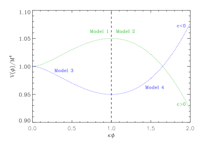
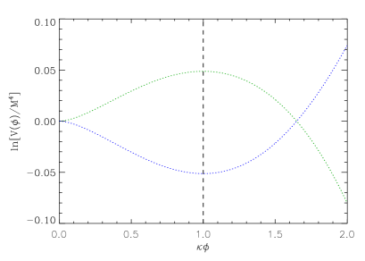
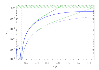
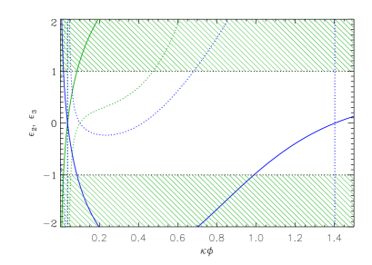
Running mass inflation can be realised in four different ways [80], denoted as RM1 to RM4, according to where the vev of the inflaton field is located along the potential, see figure 15 (top panels). RM1 corresponds to the case where $c>0$ and $\phi<\phi_{0}$. In this case, $\phi$ decreases during inflation. RM2 also corresponds to $c>0$ but with $\phi>\phi_{0}$ and $\phi$ increases during inflation. RM3 refers to the situation where $c<0$ and $\phi<\phi_{0}$ all the time. In this case, $\phi$ increases during inflation. Finally, RM4 has $c<0$ and $\phi>\phi_{0}$ decreases as inflation proceeds. Using the potential (126), one can calculate the three slow-roll parameters $\epsilon_{1}$, $\epsilon_{2}$ and $\epsilon_{3}$. Their explicit expression read

$$\epsilon_{1} = \frac{c^{2}}{2}\kappa^{2}\phi^{2}\ln^{2}\frac{\phi}{\phi_{0}}\left[1-\frac{c}{2}\left(-\frac{1}{2}+\ln\frac{\phi}{\phi_{0}}\right)\kappa^{2}\phi^{2}\right]^{-2}\,,$$ (127)

$$\epsilon_{2} = 2c\left[1+\frac{c}{4}\kappa^{2}\phi^{2}+\left(1-\frac{c}{4}\kappa^{2}\phi^{2}\right)\ln\frac{\phi}{\phi_{0}}+\frac{c}{2}\kappa^{2}\phi^{2}\ln^{2}\frac{\phi}{\phi_{0}}\right]$$ (128)

$$\times \left[1-\frac{c}{2}\left(-\frac{1}{2}+\ln\frac{\phi}{\phi_{0}}\right)\kappa^{2}\phi^{2}\right]^{-2},$$

$$\epsilon_{3} = c\ln\frac{\phi}{\phi_{0}}\left[1+\frac{c}{4}\kappa^{2}\phi^{2}+\left(1-\frac{c}{4}\kappa^{2}\phi^{2}\right)\ln\frac{\phi}{\phi_{0}}+\frac{c}{2}\kappa^{2}\phi^{2}\ln^{2}\frac{\phi}{\phi_{0}}\right]^{-1}$$ (129)

$$\times \left[1+\frac{c}{2}\kappa^{2}\phi^{2}+\frac{c^{2}}{16}\kappa^{4}\phi^{4}+c\left(2\kappa^{2}\phi^{2}+\frac{c}{2}\kappa^{4}\phi^{4}\right)\ln\frac{\phi}{\phi_{0}}\right.$$

$$+ \left.c\left(3\kappa^{2}\phi^{2}-\frac{c}{2}\kappa^{4}\phi^{4}\right)\ln^{2}\frac{\phi}{\phi_{0}}+\frac{c^{2}}{2}\kappa^{4}\phi^{4}\ln^{3}\frac{\phi}{\phi_{0}}\right]$$

$$\times \left[1-\frac{c}{2}\left(-\frac{1}{2}+\ln\frac{\phi}{\phi_{0}}\right)\kappa^{2}\phi^{2}\right]^{-2}.$$

The slow-roll parameters are represented in the bottom panels in figure 15.

Let us now study how inflation stops in these models. A priori, the end of inflation is found from the condition $\epsilon_{1}=1$ and for this reason, it is interesting to look at the behaviour of $\epsilon_{1}$ in more details (see the bottom left panel in figure 15). First of all, one notices that $\epsilon_{1}=0$ for $\phi=\phi_{0}$ (at $0.1/\kappa$ in this plot) which marks the limit between RM1 and RM3 on one side and RM2 and RM4 on the other hand. Secondly, we also remark that the curves corresponding to a model with the same value of $|c|$ are almost identical when $\kappa\phi\ll 1$. This comes from equation (127) where, in this limit, the denominator approaches unity while the numerator depends on $c^{2}$ only. If we approximate the denominator by one, then the maximum of $\epsilon_{1}$ in the range $0<\phi<\phi_{0}$ is located at $\phi\simeq\phi_{0}/e$ for which $\epsilon_{1}\simeq c^{2}\kappa^{2}\phi_{0}^{2}/(2e^{2})\ll 1$, assuming the physical values of the parameters $c$ and $\phi_{0}$ we are interested in. This means that, for RM1 and RM3, one always has $\epsilon_{1}\ll 1$ and inflation cannot stop by violation of the slow-roll conditions. Therefore, one must use another mechanism and, naturally, we will consider that inflation ends by instability at some critical value $\phi_{\mathrm{cri}}$.

In the regime where $\phi>\phi_{0}$, corresponding to RM2 and RM4, the curves representing $\epsilon_{1}$ for different $c$ but the same $|c|$ separate. From (127), one sees that this is due to the influence of the denominator. In the bottom left panel in figure 15, one notices that, for RM4, the situation is very similar to what was discussed before, i.e. inflation cannot stop due to lower than unity $\epsilon_{1}$ values. Hence, one must also use the instability mechanism for this model.

Finally, it remains RM2. For this model, the inequality $\epsilon_{1}<1$ can be violated and inflation could stop normally. In practice, this happens for large values of $\kappa\phi$ and meanwhile the other slow-roll parameters have already reached values greater than one meaning that the slow-roll approximation has already broken down. However, as long as $\epsilon_{1}<1$, inflation is still proceeding. In the following, we will also assume that inflation stops by instability (inverted hybrid mechanism).

In summary, for the four running mass models, we always consider that inflation ends at some value $\phi_{\mathrm{cri}}$ which is therefore viewed as an additional free parameter. Let us notice that, even if $\epsilon_{1}\ll 1$ while inflation is proceeding, one could have $\epsilon_{2}\gtrsim 1$ at some point [80]. In such a case, inflation would not stop but the slow-roll approximation would break down when $\epsilon_{2}=1$. As a result, the running mass inflation models under scrutiny account for a total of four primordial parameters.

We now turn to the calculation of the slow-roll parameters. Our first step is to obtain the classical trajectory, that is to say the number of e-folds in terms of the vev of the inflaton field. In the case of the running-mass model (126), it reads

$$N = \frac{1}{c}\left(\ln\left|\ln\frac{\phi}{\phi_{0}}\right|-\ln\left|\ln\frac{\phi_{\mathrm{in}}}{\phi_{0}}\right|\right)-\frac{1}{4}\left(\kappa^{2}\phi^{2}-\kappa^{2}\phi_{\mathrm{in}}^{2}\right)$$ (130)

$$+ \frac{1}{4}\left(\kappa\phi_{0}\right)^{2}\left[{\rm Ei}\left(2\ln\frac{\phi}{\phi_{0}}\right)-{\rm Ei}\left(2\ln\frac{\phi_{\mathrm{in}}}{\phi_{0}}\right)\right].$$

where the exponential integral function [31, 32] is defined by ${\rm Ei}(x)\equiv-\int_{-x}^{+\infty}{\mathrm{d}}t\rme^{-t}/t$. This expression cannot be inverted explicitly. However, in the limit $\kappa\phi\ll 1$ (which is necessary to theoretically justify the shape of the running mass potential), the above expression can be approximated by

$$N\simeq\frac{1}{c}\left(\ln\left|\ln\frac{\phi}{\phi_{0}}\right|-\ln\left|\ln\frac{\phi_{\mathrm{in}}}{\phi_{0}}\right|\right).$$ (131)

This form allows an explicit expression of the inflaton vev as a function of the number of e-folds, namely

$$\phi\left(N\right)=\phi_{0}\exp\left({\rm e}^{cN}\ln\frac{\phi_{\mathrm{in}}}{\phi_{0}}\right)\,.$$ (132)

From this expression, it is straightforward to calculate $\phi_{*}$. Remembering that inflation is supposed to stop by instability, one arrives at

$$\phi_{*}=\phi_{0}\exp\left({\rm e}^{-cN_{*}}\ln\frac{\phi_{\mathrm{cri}}}{\phi_{0}}\right)\,.$$ (133)

Equipped with this value, it is then sufficient to evaluate the slow-roll parameters for this value of the inflaton vev using the equations (127), (128) and (129).

Figure 16: Top left panel: RM1 model with $c=0.01$, $\kappa\phi_{0}=0.001$ and $10^{-9}<\kappa\phi_{\mathrm{cri}}<10^{-3.1}$. Top right panel: RM2 model with $c=0.01$, $\kappa\phi_{0}=0.001$ and $10^{-2.9}<\kappa\phi_{\mathrm{cri}}<10^{-1}$. Bottom left panel: RM3 model with $c=-0.01$, $\kappa\phi_{0}=0.001$ and $10^{-5}<\kappa\phi_{\mathrm{cri}}<10^{-3.1}$. Bottom right panel: RM4 model with $c=-0.01$, $\kappa\phi_{0}=0.001$ and $10^{-2.9}<\kappa\phi_{\mathrm{cri}}<10^{-1}$. The solid red and blues lines, as well as the blue dotted-dashed contours, have the same meaning as in figure 8.

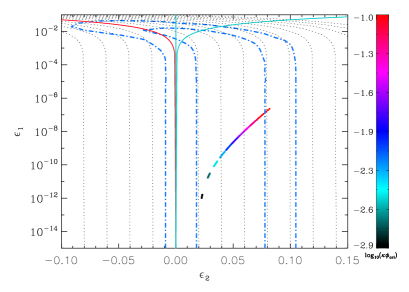
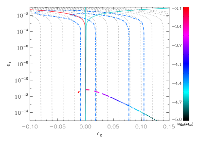
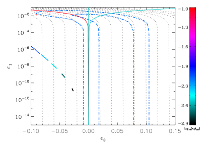
It may be interesting to present some analytical estimates of the slow-roll parameters. Instead of using the rather long equations (127), (128) and (129), one can approximate them by assuming that the denominator is just given by $M^{4}$, as done in [81, 82]. In that case, the two first order slow-roll parameters read

$$\epsilon_{1} \simeq \frac{c^{2}}{2}\left(\kappa\phi_{0}\right)^{2}\exp\left[2{\mathrm{e}}^{-cN_{*}}\ln\left(\frac{\phi_{\mathrm{cri}}}{\phi_{0}}\right)\right]{\mathrm{e}}^{-2cN_{*}}\ln^{2}\left(\frac{\phi_{\rm cri}}{\phi_{0}}\right)\,,$$ (134)

$$\epsilon_{2} \simeq 2c\left\{1+{\rm e}^{-cN_{*}}\ln\left(\frac{\phi_{\mathrm{cri}}}{\phi_{0}}\right)+c\exp\left[2{\mathrm{e}}^{-cN_{*}}\ln\left(\frac{\phi_{\rm cri}}{\phi_{0}}\right)\right]\right.$$ (135)

$$\times \left.{\mathrm{e}}^{-2cN_{*}}\ln^{2}\left(\frac{\phi_{\mathrm{cri}}}{\phi_{0}}\right)\right\}.$$

In fact, it turns out to be convenient to define the following quantity

$$s\equiv c\ln\left(\frac{\phi_{0}}{\phi_{*}}\right),$$ (136)

which can also be written as

$$s=-c\,{\mathrm{e}}^{cN_{*}}\ln\left(\frac{\phi_{\mathrm{cri}}}{\phi_{0}}\right)\,.$$ (137)

For RM1 and RM4, $s>0$ while for RM2 and RM3 one has $s<0$. This quantity can also be used to estimate $\phi_{\mathrm{cri}}$ since $\phi_{\mathrm{cri}}\simeq\phi_{0}\exp[-s\exp(-cN_{*})/c]$. Then, the approximate equations giving the first two slow-roll parameters can be re-written as

$$\epsilon_{1} \simeq \frac{s^{2}}{2}\left(\kappa\phi_{0}\right)^{2}{\rm e}^{-2s/c}\,,\qquad\epsilon_{2}\simeq 2c\left(1-\frac{s}{c}+\frac{s^{2}}{c}{\mathrm{e}}^{-2s/c}\right).$$ (138)

The last equations means that the trajectory in the plane $(\epsilon_{1},\epsilon_{2})$ can be expressed as $\epsilon_{2}\simeq 2(c-s)+4\epsilon_{1}/(\kappa\phi_{0})^{2}$. If we neglect $\epsilon_{1}$ (see below), then one recovers the formula already derived in [80, 81, 82], namely $n_{\scriptscriptstyle{\mathrm{S}}}-1\simeq 2(s-c)$. The same route for the third slow-roll parameter gives

$$\epsilon_{2}\epsilon_{3} \simeq 2c^{2}\left[-\frac{s}{c}+3c\left(\kappa\phi_{0}\right)^{2}{\mathrm{e}}^{-s/c}-3\frac{s^{3}}{c^{2}}\left(\kappa\phi_{0}\right)^{2}{\mathrm{e}}^{-2s/c}\right.$$ (139)

$$+ \left.2\frac{s^{4}}{c^{2}}\left(\kappa\phi_{0}\right)^{4}{\mathrm{e}}^{-4s/c}\right],$$

and if, again, one neglects $\epsilon_{1}$, making use of equations (58) and (62) gives the the scalar running $\alpha_{\scriptscriptstyle{\mathrm{S}}}\simeq 2sc$.

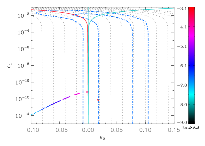
In figure 16, we have represented the slow-roll predictions for the four versions of the running mass model in the plane $(\epsilon_{1},\epsilon_{2})$, together with the $1\sigma$ and $2\sigma$ WMAP3 confidence intervals. The top left panel corresponds to the RM1 model with $c=0.01$, $\kappa\phi_{0}=0.001$ and $10^{-9}<\kappa\phi_{\mathrm{cri}}<10^{-3.1}$. The $\epsilon_{1}$ parameter appears to be extremely small and, hence, the spectral index is approximately $n_{\scriptscriptstyle{\mathrm{S}}}-1\simeq\epsilon_{2}$. According to the value of $\kappa\phi_{\mathrm{cri}}$, the spectral index can either be red for “large” values of $\kappa\phi_{\mathrm{cri}}$, i.e. $\kappa\phi_{\mathrm{cri}}$ relatively close to $\kappa\phi_{0}$, or blue for “small” values of $\kappa\phi_{\mathrm{cri}}$. The relation $n_{\scriptscriptstyle{\mathrm{S}}}-1\simeq 2(s-c)$ also reads

$$n_{\scriptscriptstyle{\mathrm{S}}}-1\simeq-2c\left[{\mathrm{e}}^{cN_{*}}\ln\left(\frac{\phi_{\mathrm{cri}}}{\phi_{0}}\right)+1\right],$$ (140)

and allows us to understand the behaviour of the spectral index.

For the RM1 model, $\phi_{\mathrm{cri}}<\phi_{0}$ and the logarithmic term in the above equation is negative. When $\phi_{\mathrm{cri}}\lesssim\phi_{0}$, this term is small, the constant term dominates in the squared bracket and, since $c>0$, the spectral index is red. When $\phi_{\mathrm{cri}}\ll\phi_{0}$, the logarithm dominates, the squared bracket is negative and the spectral index becomes blue.

The top right panel corresponds to the RM2 model with $c=0.01$, $\kappa\phi_{0}=0.001$ and $10^{-2.9}<\kappa\phi_{\mathrm{cri}}<10^{-1}$: the spectral index is always red. This can be interpreted by means of equation (140). Indeed, we now have $\phi_{\mathrm{cri}}>\phi_{0}$ and hence the squared bracket is always positive ensuring that the spectral index remains lower than unity. Moreover, the larger $\phi_{\mathrm{cri}}$, the redder $n_{\scriptscriptstyle{\mathrm{S}}}$ in agreement with what is observed.

The bottom left panel represents the RM3 model with $c=-0.01$, $\kappa\phi_{0}=0.001$ and $10^{-5}<\kappa\phi_{\mathrm{cri}}<10^{-3.1}$. The spectral index can be red or blue depending on the value of $\kappa\phi_{\mathrm{cri}}$. Since $\phi_{\mathrm{cri}}<\phi_{0}$ the logarithm term is negative. If it dominates ($\phi_{\mathrm{cri}}\ll\phi_{0}$) then the bracket in equation (140) is negative and therefore the spectrum is red since $-c>0$. On the contrary, if the constant term dominates ($\phi_{\mathrm{cri}}\lesssim\phi_{0}$), then the spectrum can be blue.

Finally, the bottom right panel corresponds to the RM4 model with $c=-0.01$, $\kappa\phi_{0}=0.001$ and $10^{-2.9}<\kappa\phi_{\mathrm{cri}}<10^{-1}$. Since $\phi_{\mathrm{cri}}>\phi_{0}$ and $-c>0$, the spectral index is always greater than one. This model can be compatible with the data only for “small” values of $\phi_{\mathrm{cri}}$ as can be seen in figure 16.

The previous observations agree with the existing literature, in particular with reference [80].

4 Testing exactly the inflationary models

In this section, we do not use the slow-roll approximation but integrate numerically both the background evolution and the cosmological perturbations. This approach allows an exact determination of the power spectra of scalar and tensor modes assuming only the linear perturbation theory in General Relativity [83, 84, 85, 86, 17]. For a given model, these power spectra depend on the parameters characterising the potential and introduced in the previous sections. By coupling this mode by mode integration during inflation to a modified version of CAMB , we can use the MCMC techniques implemented in COSMOMC to derive the constraints these parameters have to satisfy given the third year WMAP data. Let us stress that this method allows us to get marginalised posterior distributions directly on the potential parameters, out of any intermediate assumption. This approach is therefore different to the ones used so far and includes by construction a marginalisation on the reheating. As a result, the constraints we obtain include the effects coming from varying the number of efolds at which the cosmological perturbations can be generated [69, 52, 87, 5, 6, 7].

The base cosmological parameters and their priors, as well as the HST data and the top age prior, are already described in section 3.2. Therefore, in the next section, we only discuss the method used to sample the inflationary parameters.

4.1 Method

Let us sketch how the numerical integration is performed for a potential of the form $V(\phi)=M^{4}U(\phi)$.

The first step is to integrate the background evolution and this is done using the number of e-folds $N$ as time variable. The energy scale $M$ is initially set to an arbitrary non-physical value $M=1$ (see below). The initial conditions $\phi_{\mathrm{in}}$ and $\mathrm{d}\phi_{\mathrm{in}}/{\mathrm{d}}N$ are chosen such that there are at least $60$ e-folds of inflation, the end of inflation being defined to be the time at which the exact Hubble flow parameter $\epsilon_{1}=1$. Provided this condition is fulfilled, the initial conditions are in fact irrelevant thanks to the presence of the inflationary attractor [17]. Once the background integration performed, the function $\phi(N)$ is numerically known in the range $N\in[0,N_{\scriptscriptstyle{\mathrm{T}}}]$ (where $N_{\scriptscriptstyle{\mathrm{T}}}>60$ is the total number of e-folds during inflation) as well as all the other background functions, like the Hubble parameter $H(N)$.

In a second step, the equation (29) controlling the evolution of the perturbations is numerically solved. This equation is fully determined only once the time-dependent frequencies $\omega_{{\scriptscriptstyle{\mathrm{S}}},{\scriptscriptstyle{\mathrm{T}}}}(k,N)$, given in (30), are known. This requires the knowledge of $H(N)$ and its derivatives (up to third order), which simply comes from the background integration discussed above. In addition one needs the choice of some comoving wavenumbers $k$ that will be the ones of astrophysical interest today. As a result, it is compulsory to be able to relate a comoving scale $k$ during inflation to a physical scale $k_{\mathrm{phys}}$ defined at the present time. For that purpose, the complete history of the Universe needs to be specified and we now describe in more details how this can be achieved. Let us notice that equation (29), written with $N$ as time variable, takes the form

$$\frac{{\mathrm{d}}^{2}\mu_{{\scriptscriptstyle{\mathrm{S}}},{\scriptscriptstyle{\mathrm{T}}}}}{{\mathrm{d}}N^{2}}+\frac{1}{{\cal H}}\frac{{\mathrm{d}}{\cal H}}{{\mathrm{d}}N}\frac{{\mathrm{d}}\mu_{{\scriptscriptstyle{\mathrm{S}}},{\scriptscriptstyle{\mathrm{T}}}}}{{\mathrm{d}}N}+\left[\left(\frac{k}{{\cal H}}\right)^{2}-V_{\mu}(N)\right]\mu_{{\scriptscriptstyle{\mathrm{S}}},{\scriptscriptstyle{\mathrm{T}}}}=0\,,$$ (141)

where $V_{\mu}(N)$ is the effective potential for the cosmological perturbations. We see that, besides the background evolution, we need to know the quantity $k/{\mathcal{H}}$ during inflation as a function of the time variable $N$. Let us assume that we are given a physical scale today, say $k_{*}/a_{0}$ (in $\mbox{Mpc}^{-1}$ for instance), where $a_{0}$ is the present day scale factor. Then, one has

$$\frac{k_{*}}{\cal H}=\frac{k_{*}}{a_{0}H(N)}\times\frac{a_{0}}{a_{\mathrm{end}}}\times\frac{a_{\mathrm{end}}}{a(N)}\equiv\frac{\Upsilon}{H(N)}{\rm e}^{N_{{}_{\rm T}}-N}\,,$$ (142)

where $a_{\mathrm{end}}$ is the scale factor at the end of inflation and

$$\Upsilon\equiv\frac{k_{*}}{a_{0}}\frac{a_{0}}{a_{\mathrm{end}}}\,,$$ (143)

a constant which depends only on $k_{*}$ and on the history of the Universe through the ratio $a_{0}/a_{\mathrm{end}}$. In order to evaluate this constant we assume that, after inflation, there is a period of reheating as described in section 2.1.2, characterised by the two parameters $w_{\mathrm{reh}}$ and $N_{\mathrm{reh}}$, followed by a radiation dominated era that can be described by $\Omega_{\mathrm{rad}}^{0}$, followed by the matter dominated era. Let us be more precise about the reheating phase. It is interesting to consider the quantity $R_{\mathrm{rad}}$ defined by

$$\ln R_{\mathrm{rad}} \equiv \ln\left(\frac{a_{\mathrm{end}}}{a_{\mathrm{reh}}}\right)-\frac{1}{4}\ln\left(\frac{\rho_{\mathrm{reh}}}{\rho_{\mathrm{end}}}\right)=\frac{1}{4}\left(-1+3w_{\mathrm{reh}}\right)N_{\mathrm{reh}}$$ (144)

$$-\frac{1}{4}\ln\left(\frac{3+3w_{\mathrm{reh}}}{5-3w_{\mathrm{reh}}}\right)\,,$$

where $a_{\mathrm{reh}}$ and $\rho_{\mathrm{reh}}$ are respectively the scale factor and the energy density in radiation at the end of the reheating phase. This last quantity is obtained from equation (20) evaluated at $t_{\mathrm{reh}}\equiv\Gamma^{-1}$, the last term in the squared bracket being neglected. From the previous definition, one notices that $\ln R_{\mathrm{rad}}$ is exactly zero if $w_{\mathrm{reh}}=1/3$. In this case, the reheating phase cannot be distinguished from the radiation dominated era. If $-1/3<w_{\mathrm{reh}}<1/3$ then $\ln R_{\mathrm{rad}}<0$ while if $1/3<w_{\mathrm{reh}}<1$ then $\ln R_{\mathrm{rad}}>0$. For reasons that will be explained below in more details, it turns out to be convenient to define another quantity $R$

$$\ln R\equiv\ln R_{\mathrm{rad}}+\frac{1}{4}\ln\left(\kappa^{4}\rho_{\mathrm{end}}\right).$$ (145)

The quantity $\rho_{\mathrm{end}}$, the energy density stored in the scalar field at the end of inflation ($\epsilon_{1}=1$), is also completely determined once the background evolution has been solved. Therefore, if $\ln R_{\mathrm{rad}}$ is known, one can deduce $\ln R$ and vice-versa. Then, the ratio $a_{0}/a_{\mathrm{end}}$ can be written as [69]

$$\frac{a_{0}}{a_{\mathrm{end}}}=\left(\Omega_{\mathrm{rad}}^{0}\right)^{-1/4}\left(\kappa^{4}\rho_{\mathrm{cri}}^{0}\right)^{-1/4}\frac{\sqrt{\kappa^{4}\rho_{\mathrm{end}}}}{R}\,,$$ (146)

where $\rho_{\mathrm{cri}}^{0}$ is the critical energy density today, i.e.

$$\kappa^{4}\rho_{\mathrm{cri}}^{0}=3\kappa^{2}H_{0}^{2}\,.$$ (147)

Therefore, given $\rho_{\mathrm{cri}}^{0}$, $\Omega_{\rm rad}^{0}$ and $R$, i.e. a model of Universe between the end of inflation and the present time, one can calculate the constant $\Upsilon$ and hence all the terms in equation (141) are explicitly known. In practice, we implement $\ln R$ as the new inflationary parameter associated with the reheating and that is sampled from the MCMC: an uniform prior has been assumed on $\ln R$ in the range $[\ln R_{\min},\ln R_{\max}]$.

Let us discuss how the limits $R_{\min}$ and $R_{\max}$ are chosen. First of all there are limits on $\rho_{\mathrm{end}}$. In order not to spoil the success of the Big Bang Nucleosynthesis (BBN) it is reasonable to require $\rho_{\mathrm{end}}>\rho_{\mathrm{nuc}}$. Roughly speaking, this means $\rho_{\mathrm{end}}>10^{-85}m_{\scriptscriptstyle{\mathrm{Pl}}}^{4}$. On the other hand, one must have $\rho_{\mathrm{end}}<m_{\scriptscriptstyle{\mathrm{Pl}}}^{4}$ in order for the whole theoretical framework to be meaningful. In practice however, we do not need to implement this upper bound because the constraint $H_{\mathrm{inf}}/m_{\scriptscriptstyle{\mathrm{Pl}}}<1.3\times 10^{-5}$ derived in the slow-roll section (and coming from $\epsilon_{1}<0.022$) shows that the only viable perturbations have to verify $\rho_{\mathrm{end}}<10^{-10}m_{\scriptscriptstyle{\mathrm{Pl}}}^{4}$. In other words, we have

$$-187<\ln\left(\kappa^{4}\rho_{\mathrm{end}}\right)<-20\,,$$ (148)

the upper bound being not required a priori but being a consistency check that we should recover for the viable inflationary models. Now, if we use our reheating model, $R_{\mathrm{rad}}$ can be rewritten as

$$\ln R_{\mathrm{rad}}=\frac{1-3w_{\mathrm{reh}}}{12(1+w_{\mathrm{reh}})}\ln\left(\frac{\rho_{\mathrm{reh}}}{\rho_{\mathrm{end}}}\right)-\frac{1}{3\left(1+w_{\mathrm{reh}}\right)}\ln\left(\frac{3+3w_{\mathrm{reh}}}{5-3w_{\mathrm{reh}}}\right)\,,$$ (149)

where $\rho_{\mathrm{nuc}}<\rho_{\mathrm{reh}}<\rho_{\mathrm{end}}$ and $-1/3<w_{\mathrm{reh}}<1$ in order to satisfy the strong and dominant energy conditions. In this range, it is easy to see that the minimum is obtain for $w_{\mathrm{reh}}=-1/3$ and $\rho_{\mathrm{reh}}=\rho_{\mathrm{nuc}}$ whereas the maximum for $w_{\mathrm{reh}}=1$ and $\rho_{\mathrm{reh}}=\rho_{\mathrm{nuc}}$. Finally, if we use the link between $R_{\mathrm{rad}}$ and $R$, one arrives at

$$\frac{1}{4}\ln\left(\kappa^{4}\rho_{\mathrm{nuc}}\right)<\ln R<-\frac{1}{12}\ln\left(\kappa^{4}\rho_{\mathrm{nuc}}\right)+\frac{1}{3}\ln\left(\kappa^{4}\rho_{\mathrm{end}}\right),$$ (150)

up to negligible factors depending on $w_{\mathrm{reh}}$ only. In the above equation, the bounds are our definition of $\ln R_{\min}$ and $\ln R_{\max}$. Notice that these bounds explicitly depends on $\rho_{\mathrm{end}}$ which varies with the inflaton potential parameters. As a result, a “hard prior” has been coded in COSMOMC to reject any sample involving a $\ln R$ value that would not satisfy equation (150). Note that from the knowledge of $\ln R$ and $\rho_{\mathrm{end}}$, one can also derive $\ln R_{\mathrm{rad}}$ and $a_{0}/a_{\mathrm{end}}$.

From a chosen set of these parameters, the numerical integration can be straightforwardly performed to get the amplitude of the scalar and tensor power spectra at the end of inflation for any comoving wavenumber $k$ that can now be related to their corresponding physical scales today.

However, as mentioned at the beginning, this result has been obtained with an arbitrarily chosen potential scale $M=1$. In fact, the MCMC exploration is performed by directly sampling on the scalar power spectra amplitude $P_{*}$ at a given scale $k_{*}$ rather than on $M$ directly. An uniform prior has been chosen on $\ln(10^{10}P_{*})$ in the usual range $[2.7,4]$. However, one has to restore the consistency between the value of $P_{*}$ and $M$ since the former is uniquely determined by the latter. As we show in the following, a simple rescaling of the relevant functions can be used for this purpose. This rescaling has the advantage of being analytical and exact in the framework of the linear perturbation theory.

Let us consider the following rescaling for the scale $M$ or, equivalently, for the potential

$$V(\phi)\rightarrow sV(\phi)\,,$$ (151)

where $s$ is a constant. What are the consequences of this rescaling on the other quantities? From equation (11), one sees that the field $\phi(N)$ and its derivative are unaffected because only the logarithm of the potential appears in this formula. On the other hand, if we write the Friedman equation as

$$H^{2}\left[1-\frac{\kappa^{2}}{3}\left(\frac{{\mathrm{d}}\phi}{{\mathrm{d}}N}\right)^{2}\right]=\frac{\kappa^{2}}{3}V\,,$$ (152)

then one notices that the Hubble parameter transforms as $H\rightarrow s^{1/2}H$ which immediately implies that $\rho_{\mathrm{end}}\rightarrow s\rho_{\mathrm{end}}$. This also means that ${\mathcal{H}}=aH$ changes as ${\mathcal{H}}\rightarrow s^{1/2}{\mathcal{H}}$.

The previous considerations are valid for the background. Let us now see how the perturbed quantities are affected. The effective potential for cosmological perturbations, $V_{\mu}$ in equation (141), is invariant under the rescaling (151). This can be seen for instance on the gravitational waves where $V_{\mu}(N)=a^{\prime\prime}/a=1-{\cal H}^{\prime}/{\cal H}^{2}$. Therefore, requiring

$$k\rightarrow s^{1/2}k\,,$$ (153)

is sufficient to render equation (141) invariant. However, this does not mean that the amplitude itself $\mu(k,\eta)$ is not changed. Indeed, although the equation of motion is invariant, the initial conditions are modified since they read

$$\mu_{\mathrm{in}}\propto(2k)^{-1/2},\qquad\left.\frac{\mathrm{d}\mu}{\mathrm{d}N}\right|_{\mathrm{in}}\propto{\mathcal{H}}^{-1}_{\mathrm{in}}i\left(\frac{k}{2}\right)^{1/2}.$$ (154)

Because we deal with a linear equation, this implies that

$$\mu\left(k,N\right)\rightarrow s^{-1/4}\mu\left(s^{1/2}k,N\right).$$ (155)

Therefore, the scalar power spectrum evaluated at the end of inflation, i.e. at $N=N_{{}_{\rm T}}$, transforms in a very simple way, namely

$$k^{3}\left|\frac{\mu\left(k,N_{{}_{\rm T}}\right)}{a\sqrt{\epsilon_{1}}}\right|^{2}\rightarrow sk^{3}\left|\frac{\mu\left(s^{1/2}k,N_{{}_{\rm T}}\right)}{a\sqrt{\epsilon_{1}}}\right|^{2}.$$ (156)

The last step is to determine the number $s$ required to restore the consistency between our initial arbitrary normalisation $M=1$ and the values of $P_{*}$ singled out during the MCMC exploration. From the previous discussing, the required value of $s$ is simply given by the ratio $P_{*}/P^{{\scriptscriptstyle{(\mathrm{M}=1)}}}_{\diamond}$ where $P^{{\scriptscriptstyle{(\mathrm{M}=1)}}}_{\diamond}$ is the amplitude of the scalar power spectrum stemming from the mode by mode numerical integration with $M=1$ and evaluated at $k_{\diamond}=k_{*}s^{-1/2}$. Then, the final power spectra do not need to be recomputed from scratch but can be directly deduced from the transformation (156), and a similar one for the tensor modes.

In principle, the previous procedure is well-defined but the fact that the wavenumber $k$ must be continuously rescaled makes it quite difficult to implement in practice. In fact, it turns out to be more convenient to use a last trick that we now describe. The quantity $\rho_{\mathrm{reh}}$ can be viewed as an independent model parameter and, therefore, we also have the freedom to consider another model corresponding to a rescaled $\rho_{\mathrm{reh}}$. Let us consider the following transformation

$$\rho_{\mathrm{reh}}\rightarrow s^{2}\rho_{\mathrm{reh}}\,,$$ (157)

where $s$ is precisely the scaling number used in the above discussion on the rescaling of $M$. From these relations, one can immediately check that $\ln R$ (or simply $R$) is invariant whereas $R_{\rm rad}\rightarrow s^{-1/4}R_{\mathrm{rad}}$. From equation (146), this also implies that

$$\frac{a_{0}}{a_{\mathrm{end}}}\rightarrow s^{1/2}\frac{a_{0}}{a_{\mathrm{end}}}\,.$$ (158)

If we now consider the quantity $\Upsilon$ we see that its transformation under the previous rescaling is the same if we change the scale $k$ and leave $\rho_{\mathrm{reh}}$ fixed or fix the scale $k$ and change $\rho_{\mathrm{reh}}$. This is the main reason why it is more convenient to perform a MCMC sampling on the parameter $R$ rather than $R_{\mathrm{rad}}$ since at a given $R$, the rescaling required on $M$ does not induce a rescaling of the wave numbers.

In the following, we have used such an exact numerical integration of the cosmological perturbations to constrain the models previously discussed in section 3. This leads to new insights that we now describe and interpret.

4.2 Large field models

Figure 17: Marginalised posterior probability distributions (solid lines) and mean likelihood (dotted lines) for our $\Lambda$CDM base cosmological parameters together with the cosmological constant and the Hubble parameter obtained from the exact integration of large field models power spectra.

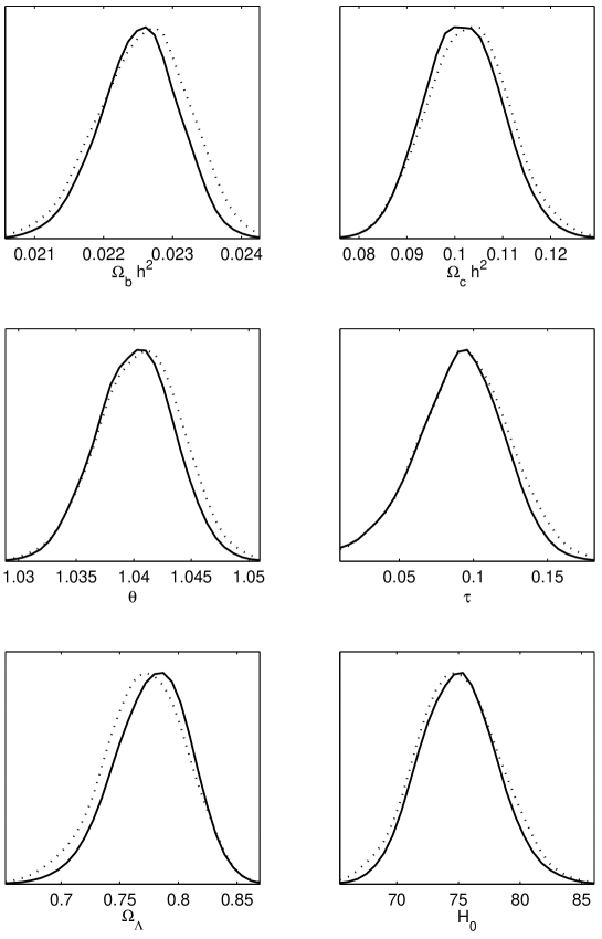
In this section, we describe the results obtained for large field models. The total number of inflationary parameters is now three: the power of the potential $p$, the potential scale $M$, which is uniquely determined from $P_{*}$, and the reheating parameter $R$. This accounts for an overall number of parameters of seven given the four base cosmological parameters. The best fit model has $\chi^{2}\simeq 11252.3$. In figure 17, we have represented the (one-dimensional) marginalised posterior probability distributions and mean likelihoods for the base cosmological parameters. As one may compare with the ones derived in the slow-roll models (see figure 2), their determination is robust and their values remain standard. This is just the consequence that, for large field models, there exists values of the primordial parameters leading to a power spectrum which allows a good fit of the data.

Figure 18: Probability distributions for the inflationary parameters characterising the large field models and the subsequent reheating period. The dotted black lines represent the mean likelihood, the solid black lines the marginalised posteriors associated with a flat prior on the index $p$, and the blue dashed lines are the marginalised posteriors coming from a flat prior on $\log p$.

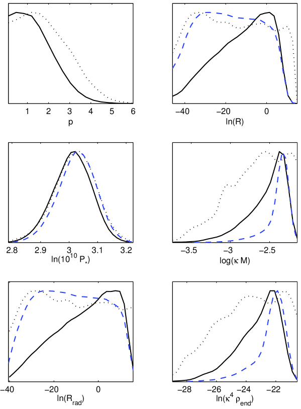
Figure 18 shows the one-dimensional posterior probabilities for the primordial parameters characterising the large field models. The corresponding two-dimensional plots are presented in figure 19. Let us recall that the quantities $p$, $\ln R$ and $P_{*}$ are directly sampled by the MCMC whereas $M$, $\ln R_{\mathrm{rad}}$, $\rho_{\mathrm{end}}$ and $a_{0}/a_{\mathrm{end}}$ are derived parameters. The curves represent the mean likelihood (dotted black line) and the marginalised probability (solid black line) obtained under a flat prior choice on $p$ in $[0.1,10]$, as well as an uniform prior on $\log p$ in $[-1,1]$ (dashed line).

One sees that models with a potential power $p\gtrsim 4$ are now strongly incompatible with the data. For values of $p$ slightly greater than, say, $3-4$, this is due a too high level of gravitational waves since the corresponding value of the spectral index $n_{\scriptscriptstyle{\mathrm{S}}}$ is still compatible with the data. For values of $p$ much larger than $3-4$, the power spectra are too red tilted and their associated $n_{\scriptscriptstyle{\mathrm{S}}}$ becomes unacceptable. At two-sigma level, one gets the upper marginalised bound

$$p<3.1\,.$$ (159)

The limiting case $p=1/10$ of our prior choice, i.e. an almost Harrison-Zeldovitch scale-invariant power spectrum, is still a non-excluded model [56, 57]. Although the maxima of the likelihood and of the marginalised probability are located around $p\simeq 1.5$ and $p\simeq 0.5$ (respectively), the model $p=1/10$ lies in the one-sigma confidence interval. This can also be seen in figure 19. The fact that values of $p<2$ are favoured can be recovered in figure 8 where the corresponding slow-roll approximation predicts a line segment below the frontier $\epsilon_{2}=2\epsilon_{1}$ (corresponding to $p=2$) in the $(\epsilon_{1},\epsilon_{2})$ plane, i.e. deeper into the $1\sigma$ confidence interval we have obtained in section 3.2.

Figure 19: Correlations between various pairs of inflationary parameters characterising the large field models and the subsequent reheating period. The coloured shaded regions represent the mean likelihoods while the solid contours trace the one and two-sigma confidence intervals of the two-dimensional marginalised posteriors.

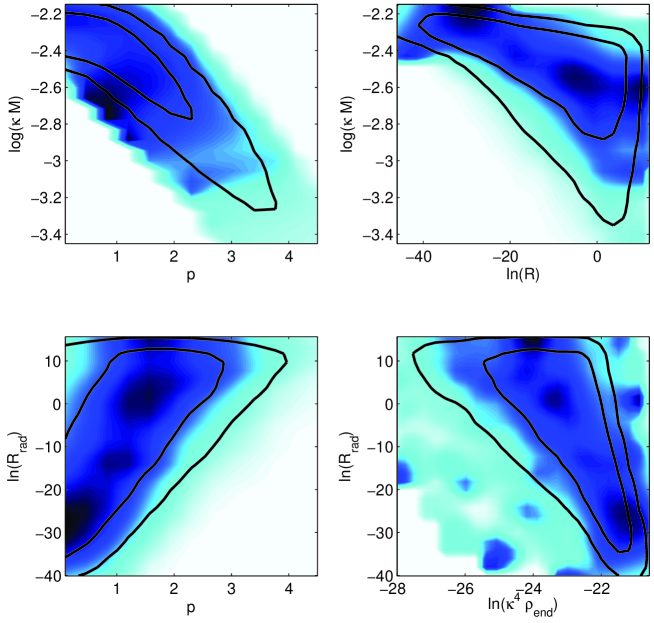
Let us now interpret the distribution obtained for the potential scale $M$. The black solid line represents its marginalised probability when a flat prior on $p$ is assumed while the blue dashed line is obtained with a flat prior on $\log p$. The fact that the two curves are significantly different signs that this parameter is poorly constrained by the data. On the other hand, the general trend is clearly the same. The value of the peak can be understood from equation (81). In fact, the degeneracies between $\log(\kappa M)$ and the index $p$ observed in figure 19 can be reproduced almost exactly using this equation from which one obtains

$$\log\left(\kappa M\right) \simeq -1.57+\frac{1}{4}\log p-\frac{1}{4}\log\left(p+4N_{*}\right)$$ (160)

$$+ \frac{p}{8}\left[1.7-\log\left(p+4N_{*}\right)-\log p\right],$$

where $N_{*}\simeq 50$.

The distribution of $\rho_{\mathrm{end}}$ can be understood in the same manner. Let us repeat that a theoretically motivated upper bound for this quantity is only $\rho_{\mathrm{end}}<m_{\scriptscriptstyle{\mathrm{Pl}}}^{4}$. We observe a sharp drop of the marginalised probability for values of $\ln(\kappa^{4}\rho_{\mathrm{end}})$ greater than $-20$. As expected and already mentioned, this is nothing but literally the constraint on the energy scale of inflation: in the slow-roll picture, $H/m_{\scriptscriptstyle{\mathrm{Pl}}}<1.3\times 10^{-5}$. With regards to the peak located at $\ln(\kappa^{4}\rho_{\mathrm{end}})\simeq-22$, it can be understood if one notices that $\rho_{\mathrm{end}}\simeq M^{4}(\phi_{\mathrm{end}}/m_{\scriptscriptstyle{\mathrm{Pl}}})^{p}$ and uses (71) with the most probable $p\simeq 1$. At two-sigma level, one gets

$$\ln\left(\kappa^{4}\rho_{\mathrm{end}}\right)<-21.3\,.$$ (161)

Let us turn to $\ln R$ and/or $\ln R_{\mathrm{rad}}$. As can be seen on the one-dimensional or two-dimensional plots, these two quantities are not constrained by the WMAP3 data. In particular, we see the strong influence of the choice of the $p$ prior. With a flat prior on $p$ (solid black line), $\ln R$ peaks around zero while with a flat prior on $\ln p$ (dashed blue line) the distribution is almost flat and cut at the edges of its prior. Let us also remind that the prior on $\ln R$ is not of top-hat shape but given by equation (150) which involves $\rho_{\mathrm{end}}$. The data are simply not accurate enough to constraint the reheating phase. Notice also that the long tails in the $M$ and $\rho_{\mathrm{end}}$ distributions are the result of their correlation with $\ln R$ through $N_{*}$ as can be seen in (160).

Figure 20: One and two-sigma confidence intervals of the three-dimensional marginalised probability distribution in the space $[(\ln\kappa^{4}\rho_{\mathrm{end}}),p,\ln R]$. The three surfaces represent the locations of constant reheating temperature $g_{*}^{1/4}T_{\mathrm{reh}}$, the values of which are indicated in the figure. They intersect along a line for $p=4$ corresponding to a reheating period with an ultra-relativistic equation of state.

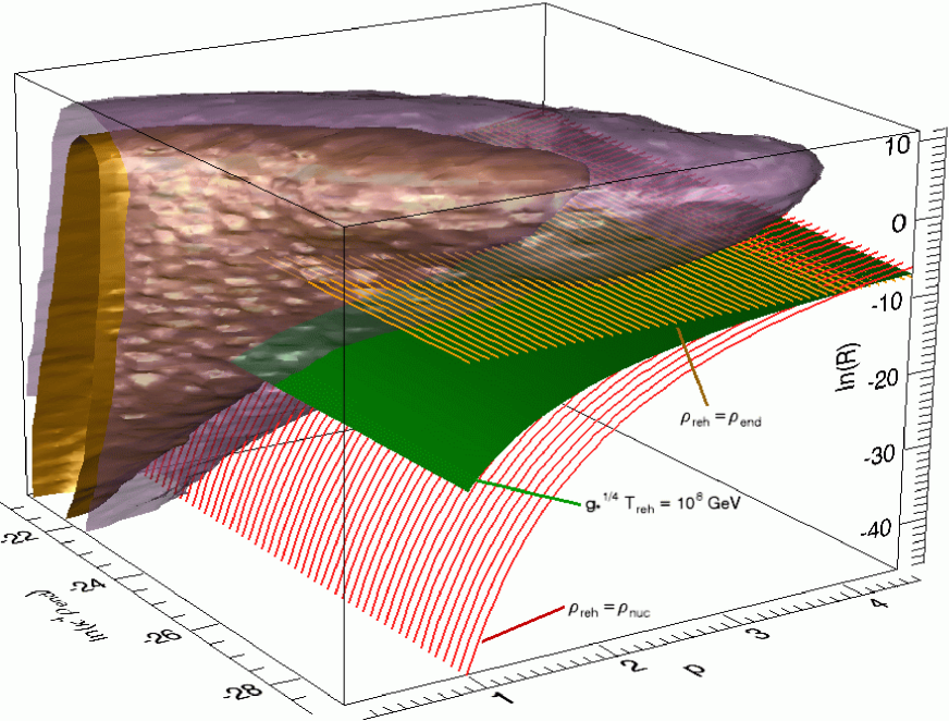
Our modelling of the reheating phase by means of $\ln R$ only can be slightly improved in the special case of the large field models. Indeed, the approach presented in section 2.1.2 turns out to be rigourous for those models with the equation of state parameter $w_{\mathrm{reh}}=P/\rho$ given by the potential power dependency $p$ through (14). If we express the reheating temperature (23) in terms of the outputs of our computations, one obtains

$$g_{*}^{1/4}T_{\mathrm{reh}} \simeq \frac{30^{1/4}}{\sqrt{\pi}}\rho_{\mathrm{end}}^{1/4}\left(\frac{3p}{p+8}\right)^{1/4}$$ (162)

$$\times \exp\left\{-\frac{3p}{p-4}\left[\ln R-\frac{1}{4}\ln\left(\kappa^{4}\rho_{\mathrm{end}}\right)+\frac{1}{4}\ln\left(\frac{3p}{p+8}\right)\right]\right\}.$$

In the space $[\ln R,\ln(\kappa^{4}\rho_{\mathrm{end}}),p]$, a given value of the reheating temperature defines a surface. In fact, the above equation can be worked out explicitly and reads

$$\ln R = \frac{p-4}{3p}\left[\ln\left(\frac{30^{1/4}}{\sqrt{\pi}}\right)-\frac{p+2}{2\left(p-4\right)}\ln\left(\frac{3p}{p+8}\right)-\ln\left(g_{*}^{1/4}\kappa T_{\mathrm{reh}}\right)\right]$$ (163)

$$+ \frac{p-1}{3p}\ln\left(\kappa^{4}\rho_{\mathrm{end}}\right).$$

The corresponding surfaces are represented in figure 20 for three values of the reheating temperature, or equivalently, for three values of $\rho_{\mathrm{reh}}$ indicated in the figure. The $1\sigma$ and $2\sigma$ confidence intervals of the three-dimensional marginalised probability have also been plotted. For convenience, we have also represented in figure 21 a few non-marginalised two-dimensional sections associated with several values of $p$. As can be seen in the three-dimensional figure, the greater $p$, the more squeezed are the lines of constant $\rho_{\mathrm{reh}}$.

Figure 21: Two-dimensional cuts of figure 20 along the planes of constant $p$. The various lines correspond to $(1/4)\ln(\kappa^{4}\rho_{\mathrm{reh}})$ equal to $-45$, $-35$, $-25$, $-15$ and $-(1/4)\ln(\kappa^{4}\rho_{\mathrm{end}})$ (bottom to top). For the case $p=4$, all the lines are merged because, in this case, $w_{\mathrm{reh}}=1/3$ and the reheating cannot be distinguished from the subsequent radiation dominated era.

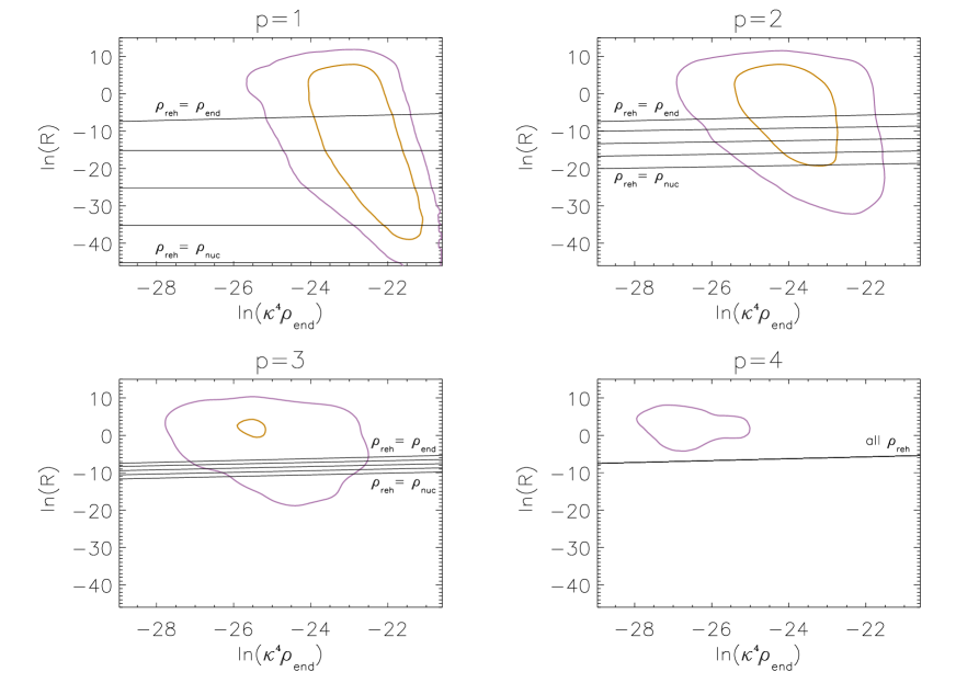
At that point, several comments are in order. Firstly, one notices that the value $p=4$ plays a particular role. In this case, equation (163) becomes $\ln R=(1/4)\ln(\kappa^{4}\rho_{\rm end})$ and $\ln R$ does no longer depend on $T_{\mathrm{reh}}$: this is why all the surfaces intersect along the corresponding line as can be seen in figure 20. This is also why there is only one line in figure 21 for the panel $p=4$. Secondly, in this last figure, one also remarks that the lines are not horizontal. According to (163), the slope is $(p-1)/(3p)$ (except for $\rho_{\mathrm{reh}}=\rho_{\mathrm{end}}$) and for $p=4$ one recovers the factor $1/4$. Thirdly, the fact that the case $p=4$ plays a special role is physically justified. The equation of state during reheating reduces to a state parameter $w_{\mathrm{reh}}=1/3$ and, as a matter of fact, the reheating phase cannot be distinguished from the subsequent radiation dominated phase. Fourthly, and as mentioned before, the slope of the lines is different if $\rho_{\mathrm{reh}}=\rho_{\mathrm{end}}$. This is because, in this case, we have an extra contribution coming from the term $\ln\left(g_{*}^{1/4}\kappa T_{\mathrm{reh}}\right)=\ln\left(g_{*}^{1/4}\kappa^{4}\rho_{\mathrm{end}}\right)/4$. This is especially visible in the top left panel of figure 21 where all the lines but the one with $\rho_{\mathrm{reh}}=\rho_{\mathrm{end}}$ are horizontal.

Let us now discuss the properties of such a reheating phase. We see in the two top panels in figure 21 that for $p=1$ and $p=2$, there are no constraint on the reheating temperature since all the lines intersect the $1\sigma$ confidence interval. For $p=1$, the central value is $\ln R\simeq-15$ and corresponds to $w_{\mathrm{reh}}=-1/3$, $g_{*}^{1/4}\kappa T_{\mathrm{reh}}\simeq 3\times 10^{-8}$ and $N_{\mathrm{reh}}\simeq 20$. For $p=1$, $\rho_{\mathrm{reh}}$ is unconstrained in the allowed range between $\rho_{\mathrm{nuc}}$ and $\rho_{\mathrm{end}}$. For $p=2$ the central value corresponds to $\rho_{\mathrm{reh}}=\rho_{\mathrm{end}}$ and, therefore, to $N_{\mathrm{reh}}\simeq 0$, while $\rho_{\mathrm{reh}}=\rho_{\mathrm{nuc}}$ is on the lower edge of the one-sigma confidence interval. Although no constraints can be put on $T_{\mathrm{reh}}$, these plots show that large field inflationary models are compatible with the data in the sense that the accelerated phase and the reheating period, which share the same field potential, can indeed coexist without leading to contradictions when confronted to the CMB observations. The cases $p=3$ and $p=4$ are slightly different since the lines of constant reheating temperature are outside the $1\sigma$ contour for $p=3$ and outside the $2\sigma$ for $p=4$. However, these models were already strongly disfavoured because of their “high” value of $p$.

4.3 Small field models

In this subsection, we study the exact numerical integration of small field models. The number of inflationary parameters is now four leading to an overall number of eight model parameters [see equation (84)]. The best fit model corresponds to $\chi^{2}\simeq 11252.2$, a value very similar to the one obtained in the large field case albeit involving the additional parameter $\mu$.

Figure 22: Mean likelihoods (dotted black lines), marginalised posterior probability distributions from a flat prior on $\kappa\mu$ in $[0.1,10]$ (thick solid black lines) and marginalised posterior probability distributions from a flat prior on $\kappa\mu$ in $[0.1,100]$ (thin solid red lines) for the $\Lambda$CDM cosmological base parameters. The cosmological constant and the Hubble parameter posteriors are also represented. They have been obtained from a direct numerical integration of the small field models power spectra.

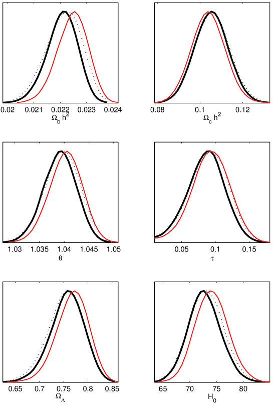
In figure 22, we have plotted the posteriors obtained for the base cosmological parameters. As previously, the dotted black curves are the mean likelihoods, the thick solid black curves represent the marginalised probabilities obtained under a flat prior on the parameter $\mu/m_{\scriptscriptstyle{\mathrm{Pl}}}$ in the range $[0.1,10]$ and, finally, the thin solid red lines refer to the marginalised probability stemming from a flat prior on $\mu/m_{\scriptscriptstyle{\mathrm{Pl}}}$ but now in the range $[0.1,100]$. The most probable values of these parameters are compatible with what was found in the slow-roll models and the exact integration of the large field models. It is nevertheless interesting to notice that the determination of these distributions is not completely insensitive to the choice on the prior. This is particularly the case for the base parameters $\Omega_{\mathrm{b}}h^{2}$ and $\tau$, which is not really surprising since both of them have significant correlations with the spectral index $n_{\scriptscriptstyle{\mathrm{S}}}$.

Figure 23: Marginalised posterior probability distributions associated with a flat prior on $\kappa\mu$ in $[0.1,10]$ (thick solid black lines) and a flat prior on $\kappa\mu$ in $[0.1,100]$ (thin solid red lines) for the primordial parameters characterising small field models and the subsequent reheating phase. The blue dashed line represents the marginalised probabilities with a flat prior on $\log(\kappa\mu)$ in $[-1,1]$ and is drawn only when it is significantly different from the others. The dotted vertical line in the top right panel indicates the relevant range of values for the $\kappa\mu\in[0.1,10]$ prior.

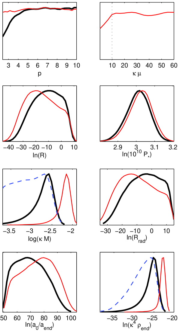
In figure 23, we have represented the posterior distributions obtained for the inflationary parameters. The conventions are the same as in figure 22. The blue dashed line is the marginalised probability with a flat prior on $\log(\mu/m_{\scriptscriptstyle{\mathrm{Pl}}})$ and is represented only when it leads to different results. On the top left panel, one sees that the parameter $p$ is not constrained since the corresponding distribution is basically flat. Let us notice that a flat prior has been chosen for $p$ in the range $[2.4,10]$, the case $p\rightarrow 2$ being very difficult to handle numerically due to computational accuracy limitation. This comes from the exponential behaviour of the $\epsilon_{1}$ parameter as we discussed in section 3.4. In fact the case $p\simeq 2$ is interesting because one notices in figure 23 that the value of the marginalised probability depends on the prior in this regime. When the flat prior on $\mu/m_{\scriptscriptstyle{\mathrm{Pl}}}$ lies in $[0.1,10]$, then the values $p\simeq 2$ are slightly disfavoured but this tendency completely disappears when the prior is extended to $[0.1,100]$. This effect can be physically interpreted by means of the slow-roll approximation presented in section 3.4. In the limit $\mu/m_{\scriptscriptstyle{\mathrm{Pl}}}\ll 1$, the first slow-roll parameter is exponentially suppressed while the second one is given by equation (102), i.e.

$$\epsilon_{2}\simeq\frac{1}{2\pi}\left(\frac{m_{\scriptscriptstyle{\mathrm{Pl}}}}{\mu}\right)^{2}.$$ (164)

In this limit, there is no means to comply with the observational constraints because $\epsilon_{2}$ becomes large which is strongly disfavoured by the data. However, as shown before, the above formula is incorrect if $\mu/m_{\scriptscriptstyle{\mathrm{Pl}}}$ is not small. When the slow-roll parameters are correctly evaluated, we have already pointed in section 3.4 that a compatible value of $\epsilon_{2}$ can be obtained provided a large enough value of $\mu/m_{\scriptscriptstyle{\mathrm{Pl}}}$ is chosen. Therefore, if the prior is too narrow, then such a large value of $\mu/m_{\scriptscriptstyle{\mathrm{Pl}}}$ cannot be reached and the case $p\simeq 2$ is disfavoured. On the other hand, if the $\mu/m_{\scriptscriptstyle{\mathrm{Pl}}}$ prior allows for large enough value, then the tilt of the power spectra can be made perfectly compatible with the data by singling out high $\mu/m_{\scriptscriptstyle{\mathrm{Pl}}}$ values. The case $p\simeq 2$ becomes perfectly compatible and, hence, the posterior distribution on $p$ flattens. Therefore, from a data analysis point of view, we conclude that the model with $p\simeq 2$ is not excluded at all. From a theoretical point of view, the situation is less clear since one could argue that the small field models require $\mu<m_{\scriptscriptstyle{\mathrm{Pl}}}$. Note that, for $p=2$, it is necessary to have $\mu/m_{\scriptscriptstyle{\mathrm{Pl}}}>0.25$ in order for the energy scale $M$ to be above the TeV (but $\mu/m_{\scriptscriptstyle{\mathrm{Pl}}}>0.03$ only for $p=2.1$). Finally, let us stress that we always have $\phi/\mu\ll 1$ and this is mandatory because the small field potential (84) should be viewed as the first leading terms of a Taylor expansion. However, this does not require $\mu/m_{\scriptscriptstyle{\mathrm{Pl}}}\ll 1$. This condition appears when one requires the vev of the inflaton field to be explicitly smaller than the Planck mass: a theoretical prior choice but of some interest since we have just shown that it modifies the $p$ posterior distribution close to $p=2$. The question of knowing whether very large inflaton vev in comparison with the Planck mass makes sense is controversial [88, 16].

The top right panel in figure 23 represents the posterior associated with the parameter $\mu/m_{\scriptscriptstyle{\mathrm{Pl}}}$. As can be seen, this parameter is basically unconstrained. The vertical dotted line is the upper limit of the posterior derived under the flat prior in the range $[0.1,10]$. In this case the respective posteriors obtained from both the prior choices match. We notice that, if one focuses on the range $[0.1,10]$ only, then there is a tendency for a “large” $\kappa\mu$, i.e. close to the upper bound $\kappa\mu\simeq 10$. As explained before, in the slow-roll language, very small values of $\kappa\mu$ are indeed disfavoured since they would lead too large values of the parameter $\epsilon_{2}$. In the full range $[0.1,100]$ the $\kappa\mu$ posterior is essentially flat and there is no significant constraint on the values of $\kappa\mu$.

Figure 24: One and two-sigma confidence contours of the two-dimensional marginalised posterior probability distributions (point density) in the plane $[\log(\kappa M),p]$ (left panel) and $[\ln(\kappa^{4}\rho_{\mathrm{end}}),\ln R_{\mathrm{rad}}]$ (right panel). The correlations with $\kappa\mu$ are indicated by the color bar.

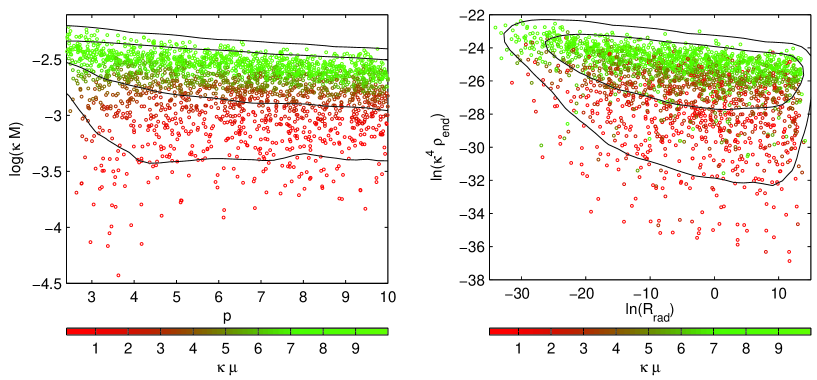
Let us now turn to the energy scale $M$ and the energy density $\rho_{\mathrm{end}}$ at the end of inflation. A first remark is that these parameters are poorly constrained and their corresponding posterior distributions are strongly dependent on the prior choice. Let us try to interpret these curves in more details making use our slow-roll understanding. If $\mu/m_{\scriptscriptstyle{\mathrm{Pl}}}\ll 1$, then, in the slow-roll approximation, the potential scale $M$ reads

$$\left(\frac{M}{m_{\scriptscriptstyle{\mathrm{Pl}}}}\right)^{4}\simeq\frac{45p^{2}}{32\pi}\frac{Q_{\mathrm{rms-PS}}^{2}}{T^{2}}\left[N_{*}\frac{p(p-2)}{8\pi}\right]^{-2(p-1)/(p-2)}\left(\frac{\mu}{m_{\scriptscriptstyle{\mathrm{Pl}}}}\right)^{2p/(p-2)}\,.$$ (165)

As already discussed in section 3.4, this energy scale can be very small. For $\mu/m_{\scriptscriptstyle{\mathrm{Pl}}}>1$, following the discussion after equation (99), one may use an approximation of equation (107) by using the limit $\phi_{*}\rightarrow 1$. One gets $\epsilon_{1}\simeq{\mathcal{O}}(1)$ which gives a very rough order of magnitude estimate (see figure 10). Finally

$$\left(\frac{M}{m_{\scriptscriptstyle{\mathrm{Pl}}}}\right)^{4}\simeq{\cal O}\left(\frac{Q_{\mathrm{rms-PS}}^{2}}{T^{2}}\right)\,,$$ (166)

that is to say $\log(\kappa M)\simeq-1.9$. This is in good agreement with what is observed in figure 23. If we use the prior $\kappa\mu$ in $[0.1,100]$ (thin red solid curve) then we allows for larger value of $\kappa\mu$ than with the prior $\kappa\mu$ in $[0.1,10]$ (thick solid black curve) and, consequently, the marginalised probability is shifted towards the large energy scales by volume effects in the parameter space. If, on the contrary, we use an uniform prior on $\log(\mu/m_{\scriptscriptstyle{\mathrm{Pl}}})$ (dashed blue line), then we favour the small values of $\mu/m_{\scriptscriptstyle{\mathrm{Pl}}}$ and the marginalised probability opens up in the direction of small $M/m_{\scriptscriptstyle{\mathrm{Pl}}}$, in accordance with the previous considerations. These ones are also confirmed by inspecting the left panel of figure 24. For a fixed value of $p$, the larger $\kappa\mu$ is, the larger $\log(\kappa M)$ becomes. Moreover, when $\kappa\mu>1$, $\log(\kappa M)$ has a very weak dependence on $p$ as one may guess from (166). Finally, let us stress that the same interpretation also applies to $\rho_{\mathrm{end}}$. In addition we recover the same cutoff at $\ln(\kappa^{4}\rho_{\mathrm{end}})\simeq-20$ as for large field models, which is once again simply the manifestation of the constraint on the level of gravitational waves, i.e. in the slow-roll language the result of $\epsilon_{1}<0.022$.

Figure 25: One and two-sigma confidence intervals (solid contours) of the two-dimensional marginalised posteriors (point density) in the plane $[\ln R,\ln(\kappa^{4}\rho_{\mathrm{end}})]$. The colour code is the same as in figure 24. The reheating predictions are represented in the particular cases where the state parameter $w_{\mathrm{reh}}=-1/3$ (top left panel), $w_{\mathrm{reh}}=0$ (top right panel), $w_{\mathrm{reh}}=1/3$ (bottom left panel) and $w_{\mathrm{reh}}=1$ (bottom right panel). The various solid lines correspond to different values of the reheating temperature $(1/4)\ln(\kappa^{4}\rho_{\mathrm{reh}})$ ranging from $-45$, $-35$, $-25$, $-15$ to $-(1/4)\ln(\kappa^{4}\rho_{\mathrm{end}})$.

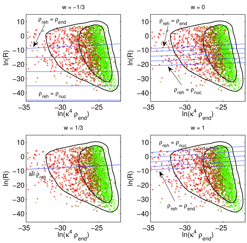
Finally, let us discuss the quantities related to the reheating phase, in particular $\ln R$. To start with, it is important to remark that contrary to the large field models, the quantities characterising the reheating phase cannot be related to the free parameters of the small field potential. In particular, the formula (14) is specific to monomial potentials and can no longer be applied to the present case. Now, from figure 23, we see that the quantity $\ln R$ has a lower bound slightly above the lower prior bound and seems to be constrained. On the contrary, the upper limit only comes from the upper bound of the prior. Let us recall that the lower limit of the prior comes from the requirement $\rho_{\mathrm{reh}}>\rho_{\mathrm{nuc}}$ which approximately means $\ln R>-46$. Here, we obtain the marginalised lower bound

$$\ln R>-34\,,$$ (167)

at two-sigma level of confidence (and $\ln R>-22$ at one-sigma). These values are obtained under the prior $\kappa\mu$ in $[0.1,100]$ which weakens the lower bound of $\ln R$ (see figure 23). The corresponding bounds for the derived parameter $R_{\mathrm{rad}}$ reads $\ln R_{\mathrm{rad}}>-31$ at $2\sigma$. Note that these constraints are recovered on the shape of the $\ln(a_{0}/a_{\mathrm{end}})$ posterior at large values. It is important to notice that these limits are modified when the prior is changed, reducing the upper bound on the $\kappa\mu$ prior would induce tighter constraints on $\ln R$. The small field models are the only class of models for which we find some non trivial, albeit weak, constraints on the reheating parameter.

Let us now try to understand the physical origin of this bound in more details. At first glance it may be surprising to get a constraint on a parameter which is not directly involved in the generation of the primordial cosmological perturbations. In fact, as we show below, this is a side-effect coming from the constraint existing on the scalar power spectrum tilt, that is to say the on the spectral index $n_{\scriptscriptstyle{\mathrm{S}}}-1$, or $\epsilon_{2}$ in the small field slow-roll approximation.

In the case of small field models, the first slow-roll parameter is extremely small. Using equation (146), one gets

$$\ln R\simeq-58+\ln\left[\frac{k}{a_{0}}\left(\mbox{Mpc}^{-1}\right)\right]+N_{k}-\frac{1}{2}\ln\frac{V_{k}}{V_{\mathrm{end}}}\,,$$ (168)

where $k/a_{0}$ is a given physical scale, $N_{k}$ the number of e-folds between the time at which the scale $k$ leaves the Hubble radius during inflation and the end of inflation, and $V_{k}$ denotes the value of the inflaton potential at Hubble exit. This equation means that $\ln R$ is directly related to the time of Hubble exit. For different values of $\ln R$, the modes of cosmological interest today probe different ranges of field value along the inflationary potential. On the other hand, not all the field values are compatible with the data, simply because in a region where the potential is too steep (or even too flat), the spectral index may take unacceptable values when compared to the observations.

One can quantitatively test the previous discussing. In practice, we choose $k/a_{0}=0.05\,\mbox{Mpc}^{-1}$, and one may approximate $V_{k}$ by $M^{4}$. Under these assumptions, the effect described before only comes from the values taken by $N_{k}$. The slow-roll value of $\phi_{\mathrm{end}}$ is known from $\epsilon_{1}(\phi_{\mathrm{end}})=1$ whereas the value of $\phi_{k}$ is obtained by solving the equation $\epsilon_{2}(\phi_{k})=\epsilon_{2}|_{\mathrm{obs}}$. Recall that the function $\epsilon_{2}(\phi)$ is explicitly given in (85) and $\epsilon_{2}|_{\mathrm{obs}}$ is supposed to be a fiducial value of the second slow-roll parameter compatible with the data. Using (93) and (94) for $\phi_{\mathrm{end}}$ and $\phi_{k}$ uniquely determines $N_{k}$ and thus $\ln R$ by means of (168). Since only a limited range of $\epsilon_{2}|_{\mathrm{obs}}$ values is compatible with the data, one indeed expect some constraints on the reheating parameter $\ln R$. For instance, all $\ln R$ values associated with $\epsilon_{2}|_{\mathrm{obs}}=0.07$ should be on the edge of the $\ln R$ marginalised posterior.

$\kappa\mu=1$
$\epsilon_{2}$	0.03	0.05	0.07
$N_{k}$	100	60	42
$\ln R$	38	-2	-19

$\kappa\mu=15$
$\epsilon_{2}$	0.03	0.05	0.07
$N_{k}$	66	34	22
$\ln R$	3	-28	-40

$\kappa\mu=50$
$\epsilon_{2}$	0.03	0.05	0.07
$N_{k}$	40	23	16
$\ln R$	-22	-39	-46

Table 1: Theoretical predicted slow-roll values of $\ln R$ for small field models with $p=4$ as a function of $\epsilon_{2}$ and for the mode $k/a_{0}=0.05\,\mathrm{Mpc^{-1}}$. Some of these values are not compatible with the data (see text).

In table 1, we have derived the expected values of $\ln R$ with respect to $\epsilon_{2}|_{\mathrm{obs}}$ in the pure slow-roll approximation for $p=4$ and for different values of $\kappa\mu$. For $\kappa\mu=15$, the value $\epsilon_{2}=0.07$ is on the edge of the confidence interval derived in section 3.2 and corresponds to $\ln R\simeq-40$: this is compatible with the drop of the $\ln R$ posterior distribution around the same value seen in figure 23. It is interesting to note that for smaller values of $\kappa\mu$, the relevant $N_{k}$ and $\ln R$ are pushed toward higher values (see table 1). This confirms that, if one has the theoretical prejudice that $\mu/m_{\scriptscriptstyle{\mathrm{Pl}}}<1$, then the bound on $\ln R$ is much tighter. Finally, to conclude this discussion, one can estimate how much the change of the $\kappa\mu$ prior propagates to the other derived parameters. From equation (146)

$$\Delta\left(\ln\frac{a_{0}}{a_{\mathrm{end}}}\right)=-\Delta\left(\ln R\right)+\frac{1}{2}\Delta\left[\ln\left(\kappa^{4}\rho_{\rm end}\right)\right],$$ (169)

and from table 1 and figure 23, we see that when one changes the prior from $\kappa\mu$ in $[0.1,10]$ to $\kappa\mu$ in $[0.1,100]$, one has $\Delta\left(\ln R\right)\simeq-10$ and $\Delta\left[\ln\left(\kappa^{4}\rho_{\mathrm{end}}\right)\right]\simeq+4$. Therefore, one gets $\Delta\left[\ln(a_{0}/a_{\mathrm{end}})\right]\simeq+12$ which is also the variation observed in the bottom left panel in figure 23.

Figure 26: Marginalised posterior probability distribution for the reheating energy scale $\ln(\kappa\rho_{\mathrm{reh}}^{1/4})$ assuming a constant state parameter $w_{\mathrm{reh}}$. For the extreme case $w_{\mathrm{reh}}=\simeq-1/3$, the small field models prefer a reheating temperature $T_{\mathrm{reh}}>2\,\mbox{TeV}$ at $95\%$ confidence level.

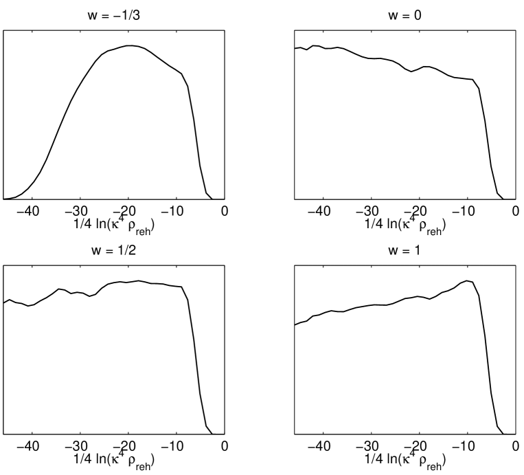
Let us now try to propagate the weak constraint on $\ln R$ to the phase of reheating itself. The reheating temperature can be evaluated as in (162) except that, as already mentioned, there is no longer a link between the state parameter $w_{\mathrm{reh}}$ and $p$. However, for a constant $w_{\mathrm{reh}}$, one still has

$$\ln\left(g_{*}^{1/4}\kappa T_{\mathrm{reh}}\right) = \frac{3+3w_{\mathrm{reh}}}{1-3w_{\mathrm{reh}}}\ln R-\frac{1+3w_{\mathrm{reh}}}{2-6w_{\mathrm{reh}}}\ln(\kappa^{4}\rho_{\mathrm{end}})$$ (170)

$$+ \frac{1}{1-3w_{\mathrm{reh}}}\ln\left(\frac{3+3\omega_{\mathrm{reh}}}{5-3w_{\mathrm{reh}}}\right)+\ln\frac{\displaystyle 30^{1/4}}{\displaystyle\sqrt{\pi}}.$$

For a fixed value of $T_{\mathrm{reh}}$ (and of $w_{\mathrm{reh}}$), equation (170) represents a line in the plane $[\ln R,\ln(\kappa^{4}\rho_{\mathrm{end}})]$. These lines are plotted in figure 25 for four values of $w_{\mathrm{reh}}$ and for the reheating temperature $(1/4)\ln(\kappa^{4}\rho_{\mathrm{reh}})$ equal to $-45$, $-35$, $-25$, $-15$, and $-(1/4)\ln(\kappa^{4}\rho_{\mathrm{end}})$. As can be seen, the bound $\ln R>-34$ does not tighten significantly the allowed $T_{\mathrm{reh}}$ values. The only lower limit that can be extracted concerns the rather extreme reheating limit $w_{\mathrm{reh}}\simeq-1/3$ for which the lines corresponding to $g_{*}^{1/4}T_{\mathrm{reh}}\lesssim 1\,\mbox{MeV}$ lie outside the two-sigma level contour over $\ln R$ and $\rho_{\mathrm{end}}$. The marginalised posteriors on $T_{\mathrm{reh}}$ can be derived by importance sampling [11] from the previous analysis and are plotted in figure 26 for four values of the parameter $w_{\mathrm{reh}}$. Notice that we have avoided the pure radiation-like case $w_{\mathrm{reh}}=1/3$ which is problematic in the inversion formula (170), as previously discussed. In the extreme case $w_{\mathrm{reh}}\simeq-1/3$, the reheating temperature satisfies

$$g_{*}^{1/4}T_{\mathrm{reh}}>2\,\mbox{TeV},$$ (171)

at $95\%$ of confidence. Of course, such a bound close to the TeV scale is already disfavored by BBN and may therefore seem irrelevant. However, we would like to point out that, in the present context, it was obtained from the CMB data only and to our knowledge, this is the first time that this can be done.

Let us conclude by noticing that, with better data (for instance coming from the Planck satellite [89]), it is likely to obtain much better constraint on the reheating temperature in the framework of small field models. As shown above, this is the result of the influence of $\ln R$ on the observed value of the the spectral index. Therefore, much tighter constraints on $n_{\scriptscriptstyle{\mathrm{S}}}$ would probably lead to a narrower range of allowed reheating temperatures.

4.4 Hybrid Models

Figure 27: Marginalised posterior probability distributions (solid black lines) and mean likelihoods (dotted lines) for the $\Lambda$CDM base cosmological parameters obtained for the hybrid models. The cosmological constant and the Hubble parameter derived posteriors are also shown.

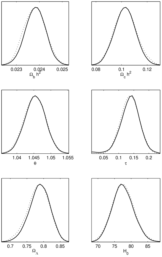
Let us now turn to the exact numerical integration of hybrid models. This class of models involves nine parameters in total, the four base cosmological parameters plus five inflationary parameters. The best fit model has a $\chi^{2}\simeq 11257.2$, a value which is larger than the one obtained for large and small field models, the difference being $\Delta\chi^{2}\simeq+5$ in spite of one extra parameter with respect to small field models and two with respect to large field models [see equation (109)]. It is therefore fair to say that this class of models does not fit the data as well as the two previous ones.

In Fig. 27, we have represented the posterior distributions for the base cosmological parameters. The most striking features of these plots are the values of the baryon number density $\Omega_{\mathrm{b}}h^{2}\simeq 0.024$, and of the optical depth, $\tau\simeq 0.14$. They should be compared to what was obtained before, say for large or small fields model where $\Omega_{\mathrm{b}}h^{2}\simeq 0.0225$ and $\tau\simeq 0.1$. In particular, such a large value of $\Omega_{\mathrm{b}}$ exacerbates the tension between the results obtained with the CMB and the BBN. Indeed, one has [90] $0.020<\Omega_{\mathrm{b}}h^{2}<0.024$ from the deuterium measurements and $0.007<\Omega_{\mathrm{b}}h^{2}<0.014$ from ${}^{7}\mbox{Li}$. Even if one considers only the Deuterium measurements, then the previous result pushes $\Omega_{\mathrm{b}}h^{2}$ towards the upper limit of the BBN allowed range.

As discussed in section 3.5 in the slow-roll context, the hybrid models are associated with a blue tilted scalar power spectrum, i.e. typically $n_{\scriptscriptstyle{\mathrm{S}}}>1$. Although not totally excluded by the WMAP data, this situation is nevertheless disfavoured. Since the parameter $n_{\scriptscriptstyle{\mathrm{S}}}$ is degenerated with the two parameters $\Omega_{\mathrm{b}}h^{2}$ and $\tau$, the more likely way to accommodate such primordial power spectra with the observed CMB anisotropies is to compensate the $n_{\scriptscriptstyle{\mathrm{S}}}>1$ values of the spectral index by modifying these two quantities. In particular, in order to compensate an excess of power at small scales (blue spectrum), one has to increase $\Omega_{\mathrm{b}}h^{2}$ and $\tau$ as observed.

Figure 28: Marginalised posterior probability distributions (solid black lines) and mean likelihoods (dotted curves) of the hybrid model inflationary parameters drawn from a flat prior on $\log\phi_{\mathrm{cri}}$ in the range $[-2,0]$. The blue dashed lines represents the marginalised posteriors obtained from an uniform prior on $\phi_{\mathrm{cri}}$ whenever they do not match with the former ones.

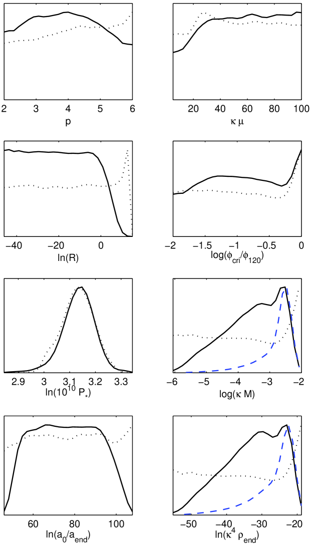
In figure 28, we have plotted the posteriors obtained for the inflationary parameters. As already discussed, the hybrid models involve an extra parameter, namely the value of the inflaton field at which the instability occurs and inflation stops. Also, we have to pay attention to probe only the vacuum dominated regime which is, by definition, what we mean by hybrid inflation. Otherwise, the situation would be very similar to the large field models studied before.

From the slow-roll analysis of section 3.5, when $\mu/m_{\scriptscriptstyle{\mathrm{Pl}}}<p/(8\sqrt{\pi})$, the field $\phi$ has to satisfy $\phi<\phi_{\epsilon}^{-}$ (see also figure 13). However, for a chosen value of $\phi_{\mathrm{cri}}$ too close to $\phi_{\epsilon}^{-}$, it is not guaranteed to obtains a total number of e-folds larger than the required $60$. In the following, we define $\phi_{120}$ to be the maximum value of $\phi_{\mathrm{cri}}$ leading to at least $120$ e-folds of inflation ($\phi$ is decreasing as hybrid inflation proceeds). In other words, $\phi_{\mathrm{cri}}$ should be smaller than $\phi_{120}$.

If $\mu/m_{\scriptscriptstyle{\mathrm{Pl}}}$ is large enough, then $\phi_{\epsilon}^{-}$ does no longer exist. In this case, $\phi_{120}$ is defined from the value of $\phi$ corresponding to the inflexion point of the potential, i.e. to $\epsilon_{2}=0$ in the slow-roll framework, which is also the field value maximising $\epsilon_{1}$. This is a convenient way to identify the vacuum dominated regime for several reasons. Firstly, $\epsilon_{2}=0$ corresponds to $\phi/\mu=1$. Therefore, the regime $\epsilon_{2}<0$ means that $\phi/\mu<1$ and, hence, the term $M^{4}$ dominates in the hybrid potential. Secondly, $\epsilon_{2}<0$ means that the kinetic energy is decreasing absolutely, and relatively to the total energy which, again, is exactly what we expect in a vacuum dominated regime. In the following, $\phi_{\mathrm{cri}}$ will be always measured in units of $\phi_{120}$.

Figure 29: Two-dimensional marginalised probability (point density) in the plane $[\log(\kappa M),p]$ for various values of $\phi_{\mathrm{cri}}$ measured in units of $\phi_{120}$ and indicated by the colour bar. The one-sigma and two-sigma confidence interval are represented by the solid contours.

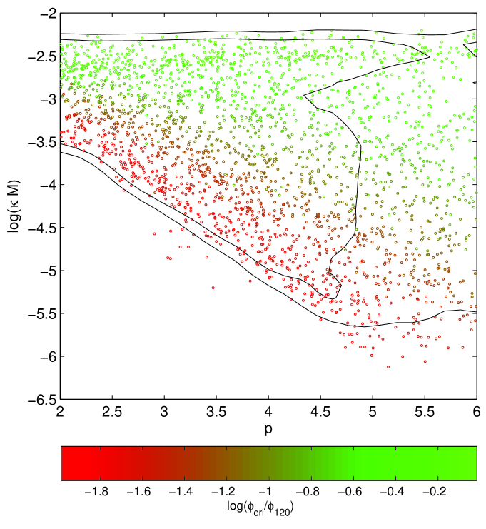
As seen in figure 28, the values of the hybrid inflationary parameters are not really constrained. The posterior distributions for $p$ or for the $\kappa\mu$ are basically flat although small values of $\kappa\mu$ are slightly disfavoured. In the same manner, the critical value $\phi_{\mathrm{cri}}$ is not constrained but values close to $\phi_{\mathrm{cri}}\simeq\phi_{120}$ seem to be slightly favoured. With regards to the energy scale $M$ and the energy density at the end of inflation, $\rho_{\mathrm{end}}$, we observe the usual cutoff for the large values of these quantities, as it was the case for large and small field models. This is still due to the constraint on the amount of gravitational waves and in terms of slow-roll, on $\epsilon_{1}$. These quantities are poorly determined as they strongly depend on the choice of the prior on $\log\phi_{\mathrm{cri}}$. In these plots, the solid black lines represent the marginalised posterior probabilities obtained with a flat prior on $\log(\phi_{\mathrm{cri}}/\phi_{120})$, whereas the dashed blue lines correspond to a flat prior on $\phi_{\mathrm{cri}}$. The order of magnitude of the results can be very simply estimated. For instance, for the scale $M$, since we are in the vacuum dominated regime, the term $(\phi/\mu)^{p}$ can be neglected and $V\simeq M^{4}$. Then, the WMAP normalisation leads to the same equation as for small field models, namely (166), which implies $M/m_{\scriptscriptstyle{\mathrm{Pl}}}\simeq 10^{-4}-10^{-2}$, in agreement with figure 28. Concerning the reheating parameter, there is no constraint at all. The distribution of $\ln R$ is flat and is only cut by the prior. This is of course the same for the posterior distribution of the derived parameter $\ln(a_{0}/a_{\mathrm{end}})$. Therefore, for the hybrid models, nothing can be said on the reheating with the WMAP3 data.

Finally, figure 29 represents the two-dimensional marginalised probability in the plane $[\log(\kappa M),p]$ for various values of $\phi_{\mathrm{cri}}$ measured in units of $\phi_{120}$. We see that the allowed range for $M$ is tighter for smaller values of $p$ and that models with large values of $\phi_{\mathrm{cri}}/\phi_{120}$ tend to have a scale $M$ larger than models with smaller $\phi_{\mathrm{cri}}/\phi_{120}$. Such an effect is expected since the potential scale $M$, in the vacuum dominated regime, is roughly given by

$$\left(\frac{M}{m_{\scriptscriptstyle{\mathrm{Pl}}}}\right)^{4}\simeq\frac{45\epsilon_{1}}{2}\frac{Q_{\mathrm{rms-PS}}^{2}}{T^{2}}\,.$$ (172)

Now, if we decrease $\phi_{\mathrm{cri}}$ then we decrease $\phi_{*}$ and hence the observed value of $\epsilon_{1}$ according to figure 13 (bottom left panel). As a result, decreasing $\phi_{\mathrm{cri}}$ implies decreasing the energy scale $M$, as observed in figure 29.

4.5 Running mass models

Figure 30: Marginalised posteriors (solid curves) and mean likelihoods (dotted) for the cosmological parameters in the running mass inflation model.

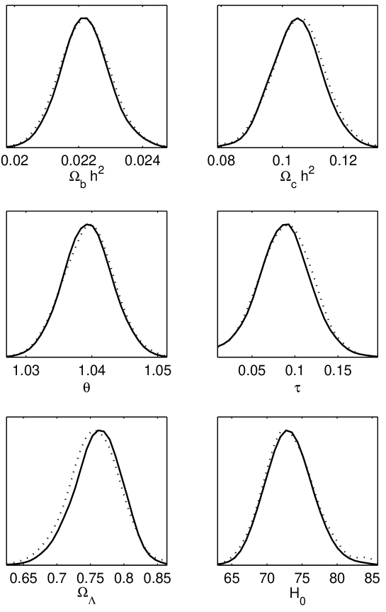
Finally, we now turn to the numerical integration of the running mass models for which the best fit parameters lead to $\chi^{2}\simeq 11252.3$. As discussed in section 3.6, these models are characterised by three additional parameters, $c$, $\phi_{0}$ and $\phi_{\mathrm{cri}}$ in comparison with the large field models. The total number of inflationary parameters is therefore five, as for the hybrid models, accounting for an overall number of nine parameters. Recall however that $\phi_{\mathrm{cri}}$ comes from the choice to stop inflation by instability and according to the different versions of this inflationary scenario, this is not always necessary.

Our numerical integration of these models appears to be limited in the parameter space due to finite accuracy issues. As pointed in section 3.6, the slow-roll approximation gives a field evolution $\phi(N)$ involving a double exponential behaviour with respect to the number of e-folds [see equation (132)]. As a result, integrating the equations of motion along $60$ e-folds may require a computing accuracy much smaller than the quadruple precision computing bound $10^{-32}$. In order to satisfy this computing requirement, we have considered a rather limited range for the MCMC running mass parameters: an uniform prior has been chosen for $\log(\kappa\phi_{0})$ in $[-3,0]$, for $c/2$ in $[-0.01,0.1]$ and for $\log(\kappa\phi_{\mathrm{cri}})$ in $[-1.8,0]$.

Figure 31: Marginalised posteriors (solid curves) and mean likelihoods (dotted) for the running mass inflationary parameters. Apart from the power spectrum amplitude $P_{*}$ and its derived parameters, these posteriors are poorly constrained by the data and mainly result from the prior choice (see text).

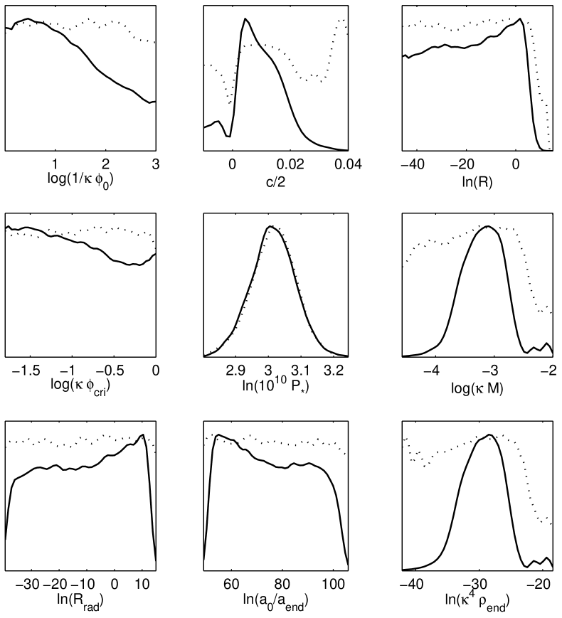
It may be convenient to compare this approach to the one used in the literature [82]. In that reference, when concerns with the leading order only, the slow-roll equations $n_{\scriptscriptstyle{\mathrm{S}}}-1\simeq 2(s-c)$ and $\alpha_{\scriptscriptstyle{\mathrm{S}}}\simeq 2sc$ are assumed. Motivated by theoretical priors, an uniform sampling on $s$ and $c$ in $[-0.2,0.2]$ is performed and used to compare the model predictions with the data, presumably by assuming a power-law power spectrum whose tilt and running are uniquely determined from the $s$ and $c$ values. An advantage of this method is that one can consider a wide range of values for the parameters $c$ and $s$. Our method differs from the fact that no assumption is made on the shape of the primordial power spectrum. Therefore, the exact numerical integration requires a sampling on the fundamental model parameters $c$, $\phi_{0}$, $\phi_{\mathrm{cri}}$. The price to pay, as mentioned before, is that the resulting domains probed by the derived parameters $s$ and $c$ are reduced to maintain the required computational accuracy.

The one-dimensional marginalised posteriors for the base cosmological parameters are plotted in figure 30 while the inflationary parameters are represented in figure 31. As for the other inflationary models which reasonably fit well the data, the cosmological parameters are centred to their fiducial values. Concerning the primordial parameters, we recover the standard bounds on the energy scale of inflation and the power spectrum amplitude, while the reheating parameters are not constrained. On the other hand, the running mass parameters exhibit distorted distributions and large values of $\phi_{0}$ seem to be favoured. A priori, the posterior on $c/2$ could be associated with some confidence intervals. However, as we show in the following, the patterns observed in figure 31 for the running mass parameters are mainly dominated by the prior choices and the multiple degeneracies that arise between the model parameters and their observable effects. This means that these parameters cannot be robustly constrained in a prior independent way with the current data, at least in our prior range.

Figure 32: Two-dimensional marginalised probability (dot density) in the plane $[\log(1/\phi_{0}),c/2]$ for various values of $\phi_{\mathrm{cri}}$ (colour bar). The one and two-sigma confidence intervals are the solid contours.

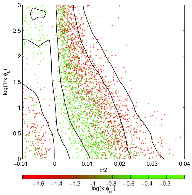
The degeneracies between the parameters are clearly drawn in the two-dimensional probability distribution (point density) plotted in figure 32. The correlations between $c/2$, $\log(\phi_{\mathrm{cri}})$ and $\log(\phi_{0})$ appear as the preferred “islands” and “directions” explored by the MCMC. The topology of these correlations can be understood from the slow-roll approximation detailed in section 3.6. Indeed, since $\epsilon_{1}$ is generically small for this class of models, equation (138) implies $1-n_{\scriptscriptstyle{\mathrm{S}}}\simeq\epsilon_{2}$. Since the spectral index $n_{\scriptscriptstyle{\mathrm{S}}}$ is constrained by the data, one can recover the range of model parameters that lead to such an observed value of $n_{\scriptscriptstyle{\mathrm{S}}}$, or $\epsilon_{2}$ in the present case.

From the expression of $s$ derived in (137), a given value of $\epsilon_{2}$ defines a surface in the three-dimensional volume $[\log(\kappa\phi_{\mathrm{cri}}),c/2,\log(1/\kappa\phi_{0})]$ given by

$$\log(\kappa\phi_{\mathrm{cri}})=\mathrm{e}^{-cN_{*}}\left[1-\frac{\epsilon_{2}}{4}\left(\frac{c}{2}\right)^{-1}-\log\left(\frac{1}{\kappa\phi_{0}}\right)\right]\,,$$ (173)

for a given $N_{*}$. This equation explicitly gives the degeneracies between the running mass parameters leading to the same $\epsilon_{2}$ values. However, it is only an approximate solution of the slow-roll equations valid as long as $\kappa\phi\ll 1$ and some precautions should be in order when dealing with the RM4 and RM2 models. In fact, one may alternatively invert (130) numerically for a given $N_{*}$ and use the equation (128) to recover the surfaces of constant $\epsilon_{2}$. These surfaces are represented in figure 33 for three values of $\epsilon_{2}$ corresponding to the mean value ($\epsilon_{2}=0.034$) and to the two-sigma confidence bounds ($\epsilon_{2}=-0.029$ and $\epsilon_{2}=0.074$) obtained for the second order slow-roll expansion and under the Jeffreys’ prior on $\epsilon_{1}$. If we compare figure 32 with figure 33, we recover that the MCMC spread out along the surfaces associated with $\epsilon_{2}\simeq 0.034$.

Figure 33: Isosurfaces of constant $\epsilon_{2}$ in the three-dimensional parameter space of the running mass inflation model. The blue surface is associated with $\epsilon_{2}=-0.029$ and the dark red one with $\epsilon_{2}=0.074$. These two values correspond to the two-sigma confidence intervals at next-to-leading order in slow-roll expansion and for the Jeffreys’ prior on $\epsilon_{1}$. The yellow surface corresponds to $\epsilon_{2}=0.034$. The black mesh corresponds to $\phi=\phi_{0}$ and marks the border between RM1, RM3 on one hand and RM2, RM4 on the other hand. Finally, the region $c>0$ corresponds to RM1 and RM2 while $c<0$ contains RM3 and RM4. The value $N_{*}=40$ has been used.

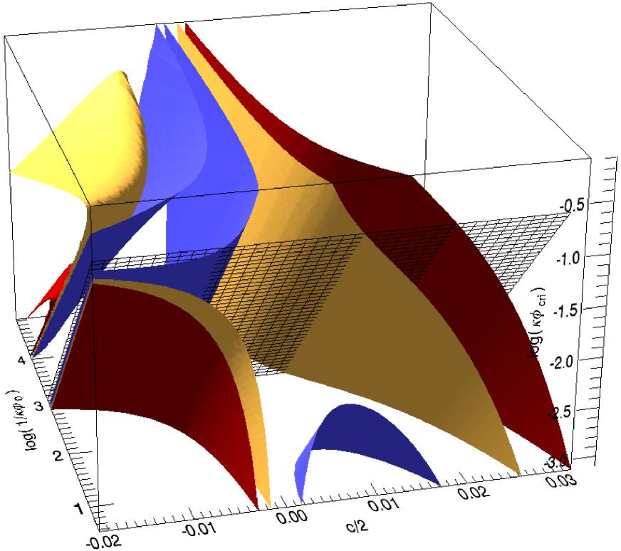
Firstly, let us notice that the folded yellow surface in the region $-\log(\kappa\phi_{0})\simeq 4$, $c<0$ corresponds to models with small values of $\kappa\phi_{\mathrm{cri}}$ and $\kappa\phi_{0}$ but (and this cannot be seen in the figure) with large values of $\kappa\phi_{\mathrm{in}}$ (this is the RM4 model). These models are compatible with the data but they may suffer a theoretical inconsistency since they are associated with vev larger than the Planck mass as inflation proceeds. Note that these parts of the yellow surface cannot be found by using (173) since its domain of validity breaks down in that particular case.

Figure 33 demonstrates that the constraints appearing on the one and two-dimensional marginalised probabilities on the running mass parameters are mainly due to a preferential volume selection in the parameter space by the prior choice. Indeed, if one would extend the range of $\log(\kappa\phi_{\mathrm{cri}})$ below $-3$, then the dark red surface would penetrate the region of higher $c$ values and would render these $c$ values compatible with the data. The conclusion is similar for the blue inverted half-pipe around the value $c=0$. Extending the prior of $\kappa\phi_{\mathrm{cri}}$ and $\kappa\phi_{0}$ would render the region around $c=0$ compatible with the data. However, the strong variations of $\kappa\phi_{\mathrm{cri}}$ and $\kappa\phi_{0}$ required to get a reasonable value of $\epsilon_{2}$ for an arbitrarily chosen $c$ suggest that some amount of fine-tuning is required between these parameters.

Nevertheless, for the running mass models, the main conclusion is that the dependence on the priors prevents us to establish reliable constraints on the free parameters. To avoid this difficulty, it would be necessary to integrate numerically the spectrum for very small values of $\kappa\phi_{\mathrm{cri}}$ and $\kappa\phi_{0}$ but, as noticed at the beginning of the section, this is a non-trivial technical issue and some theoretical lower bound should also be set. On the other hand, one can say that these models remain compatible with WMAP3 data.

5 Are the power spectra really featureless?

5.1 Basic equations

Recently, the possibility that the power spectra could contain non-expected features has been widely discussed. This question arose because of the presence of the so-called cosmic variance outliers in the first year WMAP data. Since these litigious points have disappeared (at least some of them) in the new data, it seems at first sight that this is no longer an interesting issue. This conclusion is also consistent with the analysis of the WMAP team [2] which quotes a $\chi^{2}$ drop of $\Delta\chi^{2}\simeq-4.5$ or $\Delta\chi^{2}\simeq-9.5$ according to the type of features considered. Notice that, although $\Delta\chi^{2}\simeq-4.5$ seems indeed not of much interest, $\Delta\chi^{2}\simeq-9.5$ deserves at least some attention. In this article, we would like to consider this question further and derive the marginalised bound the parameters associated with these features satisfy. A tool that has been used in order to address this issue is to confront the trans-Planckian power spectra to the CMB data. The trans-Planckian problem originates from the fact that, due to the exponential expansion during inflation, the scales of astrophysical interest today were below the Planck length at the beginning of inflation [91, 92, 93, 94, 95, 96, 97, 98, 99, 100, 101, 102, 103, 104, 105, 106, 107, 108, 109, 110, 111, 112, 113, 114, 115, 116, 117]. In this regime, the framework utilised to derive the inflationary predictions (namely quantum field theory in curved space-time) breaks down. This is similar to what happens in the context of black hole physics and the derivation of the Hawking radiation [118, 119, 120]. If we denote $M_{\mathrm{c}}$ the physical scale at which new physical effects are supposed to become relevant, one finds that superimposed oscillations appear in the power spectra the amplitude of which is controlled by the $H$ to $M_{\mathrm{c}}$ ratio, the only two scales available in the theory. These superimposed oscillations are then tested against the data and used as a tool to detect non-trivial features in the primordial power spectrum [126, 127, 128, 129, 130, 131, 132, 133, 134, 135].

It was shown in Ref. [107, 129, 131, 130] that a crucial point is the fact that the amplitude and the frequency of the oscillations are independent quantities. Since this question was sometimes not fairly appreciated in the recent literature, we would like to briefly review where this comes from. In particular, we argue that considering dependent amplitude and frequency is theoretically not justified in the framework of the so-called “minimal approach”. Moreover, postulating that the amplitude is inversely proportional to the frequency is phenomenologically restrictive since this has the consequence that the region of interest in the parameter space is missed.

In the minimal approach, only the initial conditions for the primordial perturbations are modified while their equation of motion is left unchanged (this would no longer be the case if, for instance, we had modelled the new physical effects by a modified dispersion relation). The initial conditions are not the standard ones because they are fixed when the wavelength of a given Fourier mode becomes equal to a new fundamental characteristic scale $\ell_{\mathrm{c}}$. The time $\eta_{k}$ of mode “appearance” associated with a comoving wavenumber $k$ stems from the condition

$$\lambda(\eta_{k})=\frac{2\pi}{k}a(\eta_{k})=\ell_{\mathrm{c}}\equiv\frac{2\pi}{M_{\mathrm{c}}}\,,$$ (174)

which implies that $\eta_{k}$ is a function of $k$. Therefore, this is different from the standard inflationary calculations where the initial time is taken to be $\eta_{k}=-\infty$ for any Fourier mode $k$ and where, in a certain sense, the initial time does not depend on $k$. This additional $k$-dependence is at the origin of the appearance of the superimposed oscillations. Another crucial question is in which state the Fourier mode is placed at the time $\eta_{k}$. At this point, one would like to be as general as possible and we take

$$\mu_{{\scriptscriptstyle{\mathrm{S}}},{\scriptscriptstyle{\mathrm{T}}}}(\eta_{k}) = \mp\frac{c_{k}+d_{k}}{\sqrt{2\omega_{{\scriptscriptstyle{\mathrm{S}}},{\scriptscriptstyle{\mathrm{T}}}}(\eta_{k})}}\frac{4\sqrt{\pi}}{m_{\scriptscriptstyle{\mathrm{Pl}}}}\,,$$ (175)

$$\mu_{{\scriptscriptstyle{\mathrm{S}}},{\scriptscriptstyle{\mathrm{T}}}}^{\prime}(\eta_{k}) = \pm i\sqrt{\frac{\omega_{{\scriptscriptstyle{\mathrm{S}}},{\scriptscriptstyle{\mathrm{T}}}}(\eta_{k})}{2}}\frac{4\sqrt{\pi}(c_{k}-d_{k})}{m_{\scriptscriptstyle{\mathrm{Pl}}}}\,.$$ (176)

The coefficients $c_{k}$ and $d_{k}$ are a priori two arbitrary complex numbers satisfying the condition $|c_{k}|^{2}-|d_{k}|^{2}=1$. Without restricting the physical content of the problem, and given the fact that, in the limit $M_{\mathrm{c}}\rightarrow+\infty$, one must recover the standard limit, i.e. the Bunch-Davies vacuum, one typically expects that

$$c_{k} = 1+y_{k}\sigma_{0}+\dots\,,\qquad d_{k}=x_{k}\sigma_{0}+\dots\,,$$ (177)

where $\sigma_{0}\equiv H/M_{\mathrm{c}}$. Any other particular choice would be a strong assumption to be justified. The only simplification that one may consider is to assume that $x_{k}\simeq x$ and $y_{k}\sim y$, that is to say that these two coefficients are not strongly scale dependent in the range of scales under consideration. In the following, the parameters $x$ and $y$ are considered as free parameters that are not fixed by any existing well-established theories except that, of course, they should satisfy $|c_{k}|^{2}-|d_{k}|^{2}=1$. This implies that the amplitude and the frequencies of the superimposed oscillations are independent quantities as announced. Finally, the form of the power spectra stemming from the previous considerations read, for the scalar modes [108, 129]

$$k^{3}P_{\zeta} = \frac{H^{2}}{\pi\epsilon_{1}m_{\scriptscriptstyle{\mathrm{Pl}}}^{2}}\left\{1-2(C+1)\epsilon_{1}-C\epsilon_{2}-\left(2\epsilon_{1}+\epsilon_{2}\right)\ln\frac{k}{k_{*}}\right.$$ (178)

$$- \left.2|x|\sigma_{0}\left[1-2(C+1)\epsilon_{1}-C\epsilon_{2}-\left(2\epsilon_{1}+\epsilon_{2}\right)\ln\frac{k}{k_{*}}\right]\right.$$

$$\times \left.\cos\left[\frac{2}{\sigma_{0}}\left(1+\epsilon_{1}+\epsilon_{1}\ln\frac{k}{a_{0}M_{\mathrm{c}}}\right)+\varphi\right]\right.$$

$$- \left.|x|\sigma_{0}\pi\left(2\epsilon_{1}+\epsilon_{2}\right)\sin\left[\frac{2}{\sigma_{0}}\left(1+\epsilon_{1}+\epsilon_{1}\ln\frac{k}{a_{0}M_{\mathrm{c}}}\right)+\varphi\right]\right\},$$

and for the gravitational waves

$$k^{3}P_{h} = \frac{16H^{2}}{\pi m_{\scriptscriptstyle{\mathrm{Pl}}}^{2}}\left\{1-2(C+1)\epsilon_{1}-2\epsilon_{1}\ln\frac{k}{k_{*}}\right.$$ (179)

$$- \left.2|x|\sigma_{0}\left[1-2(C+1)\epsilon_{1}-2\epsilon_{1}\ln\frac{k}{k_{*}}\right]\right.$$

$$\times \left.\cos\left[\frac{2}{\sigma_{0}}\left(1+\epsilon_{1}+\epsilon_{1}\ln\frac{k}{a_{0}M_{\mathrm{c}}}\right)+\varphi\right]\right.$$

$$- \left.2|x|\sigma_{0}\pi\epsilon_{1}\sin\left[\frac{2}{\sigma_{0}}\left(1+\epsilon_{1}+\epsilon_{1}\ln\frac{k}{a_{0}M_{\mathrm{c}}}\right)+\varphi\right]\right\},$$

where $\varphi$ is the argument of the complex number $x$, i.e. $x\equiv|x|{\rm e}^{i\varphi}$. We see that the new power spectra depend, at most, on three new independent parameters, namely the amplitude, the frequency and the phase of the superimposed oscillations. In particular, their wavelength can be expressed as

$$\frac{\Delta k}{k}=\frac{\sigma_{0}\pi}{\epsilon_{1}}\,.$$ (180)

The derivation of the trans-Planckian corrections in the power spectra (178) and (179) assumes that the back-reaction effects are not too important. For consistency, the energy density of the perturbations must be smaller or equal than that of the inflationary background. This leads to the condition $|x|\leq\sqrt{3\pi}m_{\scriptscriptstyle{\mathrm{Pl}}}/M_{\mathrm{c}}$, an estimate which is in agreement with the one derived in [107]. In order to put numbers on the above constraint, we can use equations (66) and (67) together with $M_{\mathrm{c}}=H/\sigma_{0}$ to arrive at

$$|x|\sigma_{0}\leq 10^{4}\times\frac{\sigma_{0}^{2}}{\sqrt{\epsilon_{1}}}\,,$$ (181)

where, in order to derive an order of magnitude estimate, the unimportant factors of order one have been neglected. It is important to emphasise that the above constraint is only a sufficient condition, but by no means, unless proven otherwise, a necessary condition for the validity of the power spectra calculations [110].

5.2 WMAP constraints on the oscillatory parameters

In order to test the viability of superimposed oscillations in the primordial power spectra, we perform an exploration of the primordial parameter space by using MCMC methods implemented in COSMOMC , given the third year WMAP data. Our analysis proceeds in two steps. In a first part, the trans-Planckian power spectra in (178) and (179) are used to seed the CMB anisotropies in the framework of the first order slow-roll expansion (see section 3.2.1). In a second part, we reiterate the analysis by using a power law primordial power spectrum supporting a wider class of superimposed oscillations, namely oscillating with a $k/k_{*}$ power-law dependence. As detailed in [129, 130, 131], we use a modified version of CAMB to compute the CMB anisotropies whose required accuracy and computational time renders impossible an exploration of the full parameter space. Along the lines drawn in those references, only the primordial parameter space is probed while the base cosmological parameters remain fixed to their best fit values obtained from an MCMC analysis without superimposed oscillations.

5.2.1 Trans-Planckian power spectra

Figure 34: Marginalised posterior probability distributions (solid right stairs) and mean likelihood (shaded bars) for the trans-Planckian primordial parameters. Note that these posteriors are derived under a fix set of cosmological parameters.

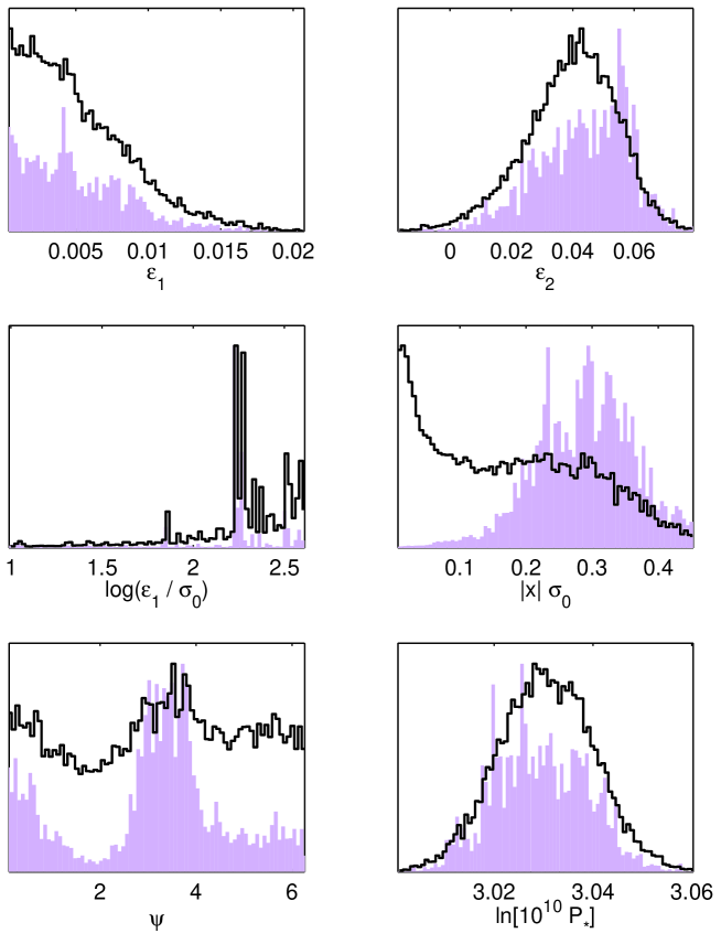
As described in the previous section, in addition to the first order Hubble-flow parameters $\epsilon_{1}$ and $\epsilon_{2}$, the scalar power spectrum amplitude at the pivot scale $P_{*}$, considering the trans-Planckian power spectra (178) and (179) accounts for three more primordial parameters. We have chosen uniform priors on the overall oscillatory phase $\psi$ in $[0,2\pi]$, defined as

$$\psi\equiv\frac{2}{\sigma_{0}}\left(1+\epsilon_{1}\right)+\varphi,$$ (182)

as well as on the parameter $|x|\sigma_{0}$ in $[0,0.45]$. Moreover, in order to sample directly from the oscillation frequency, an uniform prior has been chosen on the parameter $\log(\epsilon_{1}/\sigma_{0})$ in $[1,2.6]$. The other primordial parameters are sampled according to the uniform prior choice on $\epsilon_{1}$ described in section 3.2.1.

The converged posteriors for the primordial parameters have been plotted in figure 34. As previously mentioned, they have been obtained for a set of fixed cosmological parameters $\Omega_{\mathrm{b}}h^{2}=0.021$, $\Omega_{\mathrm{dm}}h^{2}=0.0159$, $\theta=1.0393$ and $\tau=0.0942$ (implying $H_{0}\simeq 72\,\textrm{km/s/Mpc}$) and the MCMC exploration has been stopped after approximately $200000$ elements for which the generalised Gelman and Rubin $R$–statistics implemented in COSMOMC  [11, 136] is less than $10\%$. The constraints obtained on the standard primordial parameters $\epsilon_{1}$, $\epsilon_{2}$ and $P_{*}$ are stronger than those derived in section 3.2.1, as expected since the cosmological parameters have been fixed to their best fit values.

The overall constraint on trans-Planckian superimposed oscillations is given by the $|x|\sigma_{0}$ marginalised posterior. The vanishing value of this quantity corresponds to the standard first order slow-roll primordial power spectra without oscillation and is still the favoured model given the third year WMAP data. However, as it was the case with the first year data [131], the mean likelihood is peaked over non-vanishing values of $|x|\sigma_{0}$ showing that superimposed oscillations provide a better fit to the data. As detailed in [131], the marginalised posterior remains peaked around vanishing values due to volume effects in the parameter space: the best fit region occupies a rather limited volume that does not take over the accessible volume associated with the non-oscillatory models in spite of their lower likelihoods. Nevertheless, the statistical weight coming from the highest likelihood values broadens out the posterior distribution on $|x|\sigma_{0}$ and at two-sigma level one has

$$|x|\sigma_{0}<0.38\,.$$ (183)

This number has to be compared with the limit derived in [131], namely $|x|\sigma_{0}<0.11$. The best fit volume confinement in the parameter space may be understood on the marginalised posterior associated with the frequency parameter $\log(\epsilon_{1}/\sigma_{0})$. As can be seen in figure 34, both the mean likelihood and marginalised probability exhibits narrow peaks on particular frequencies only thereby leading to a discrete set of best fit sub-manifolds in the parameter space. From the WMAP team likelihood code [1, 2, 3, 4], the best fit associated with the highest resonance peak leads to an overall $\chi^{2}=11239.9$, which is a fit improvement of $\Delta\chi^{2}\simeq-12$ with respect to the first order vanilla slow-roll model, for three additional parameters (see figure 35). Note that this value is larger that the one reported by the WMAP team [2], possibly due to the localisation of the highest likelihood resonance in a rather high frequency region $\log(\epsilon_{1}/\sigma_{0})\simeq 170$.

Figure 35: In the left panel, smoothed one and two-sigma contours (solid line) of the two-dimensional marginalised posterior probability distributions (coloured dots) in the plane $[\log(\epsilon_{1}/\sigma_{0}),|x|\sigma_{0}]$. The highest probable frequencies clearly appear as the vertical coloured dot alignments. The right panel represents the cumulative residual $\chi^{2}$ between the trans-Planckian best fit model and the vanilla first order slow-roll model.

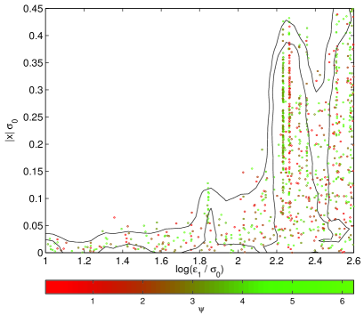
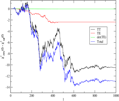
Eventually, compared to the first year WMAP data, we still find no evidence for superimposed oscillations in the WMAP third year data. However, considering trans-Planckian-like superimposed oscillations still significantly improves the fit to the data, and more importantly the overall statistical weight associated with these best fit regions has increased.

Let us now study what the above results imply for trans-Planckian physics. As already mentioned, the best fit is obtained for $\log(\epsilon_{1}/\sigma_{0})\simeq 2.23$, $\epsilon_{1}\simeq 2.1\times 10^{-3}$ and $|x|\sigma_{0}\simeq 0.268$. This implies $\sigma_{0}\simeq 1.2\times 10^{-5}$. Moreover, if one uses the value of $\epsilon_{1}$ for the best fit (this does not mean, of course, that we have detected a non-vanishing $\epsilon_{1}$ since this would imply a detection of primordial gravitational waves), then one can estimate $M_{\mathrm{c}}$ which reads $M_{\mathrm{c}}\simeq 0.3m_{\scriptscriptstyle{\mathrm{Pl}}}$. Some serious problems show up when one tries to see whether the best fit suffers from a back-reaction problem. Using equation (181), one finds that this is not the case provided $|x|\sigma_{0}\leq 3.3\times 10^{-5}$. This limit is thus largely violated by the best fit. At this point, several remarks are in order. Firstly, strictly speaking, this results clearly invalidates the perturbative framework used in order the derived the power spectra with the superimposed oscillations. Secondly, as discussed in [110, 117], the back-reaction is not necessarily a problem as its effect might just “renormalise” the vacuum energy during inflation. In other words, it may not necessarily prevent inflation to proceed. Thirdly, the presence of superimposed oscillations is not necessarily linked to trans-Planckian effects. In that case, the limit given by equation (181) simply does not apply. But, then, it becomes more difficult to physically motivate the logarithmic shape of the oscillations which turns out to be favoured by the data (see below).

To conclude this section we would like to describe a few intriguing features, although not statistically significant, that appears in the previous analysis. As shown in [137], it is worth stressing that multiple resonances in the likelihood are precisely expected in presence of an oscillatory signal due to “frequency beating” between the data and the model tested. These degeneracies produce a multi-valued function in the recovery of a primordial oscillation frequency, but also open a window on the a priori unobservable high frequency signals through their lower frequency resonances. Compared to the first year data, we find the appearance of new favoured frequencies that can be seen as the peaks in the $\log(\epsilon_{1}/\sigma_{0})$ posterior of figure 34, or through the dot alignments in figure 35. Another intriguing feature concerns the marginalised posterior and the mean likelihood of the phase parameter $\psi$. As can be seen in figure 34, values around $\psi\simeq 0$ and $\psi\simeq 3$ are slightly favoured by the data (once again, not in a statistically significant way). As shown in [129], in presence of high frequency oscillations, $\psi=\pi$ modulo $\pi$ are the phase values expected to maximise the oscillation amplitude in the multipole moments. As already mentioned, even in presence of an oscillatory signal in the data, one cannot conclude that it comes from a primordial origin and it may be the result of some foreground contamination. However, one would have to explain how such a pattern in the inter-multipole correlations arises.

5.2.2 Power law power spectrum

In this section, we reiterate the previous analysis by using a phenomenological primordial power spectrum. Only the scalar modes have been considered with a power spectrum of the form [128]

$$k^{3}P_{\zeta}=P_{*}\left(\frac{k}{k_{*}}\right)^{n_{\scriptscriptstyle{\mathrm{S}}}-1}\left(1-A_{\omega}\cos\left\{\frac{\omega}{p}\left[\left(\frac{k}{k_{*}}\right)^{p}-1\right]+\psi\right\}\right).$$ (184)

In the limit $p\rightarrow 0$, one recovers logarithmic-like dependence in the oscillation frequency. The interest of this kind of power spectrum resides in the comparison of models having superimposed oscillations with a different frequency dependence in the wave number $k$. In other words, one can test whether the logarithmic oscillations are special or if any oscillatory signal can significantly improve the best fit. For the sake of simplicity, we have not considered a running spectral index and, as in the previous section, only the primordial parameter space has been explored once the cosmological parameters have been fixed to their best fit value obtained from the fiducial power law scalar power spectrum: $\Omega_{\mathrm{b}}h^{2}=0.0223$, $\Omega_{\mathrm{dm}}=0.1064$, $\theta=1.040$ and $\tau=0.0885$. An uniform prior has been chosen for $\log(p)$ in the range $[-5,0.48]$ (the upper bound corresponds to $p\simeq 3$) as well as for $\log(\omega)$ in $[1,2.5]$. The phase $\psi$ is sampled from a flat prior in $[0,\pi]$ and $n_{\scriptscriptstyle{\mathrm{S}}}$ from the range $[0.5,1.5]$, also with an uniform prior.

Figure 36: Marginalised posterior probability distributions (solid right stairs) and mean likelihood (shaded bars) for the oscillatory power law parameters. Note that this posteriors are derived under a fix set of cosmological parameters.

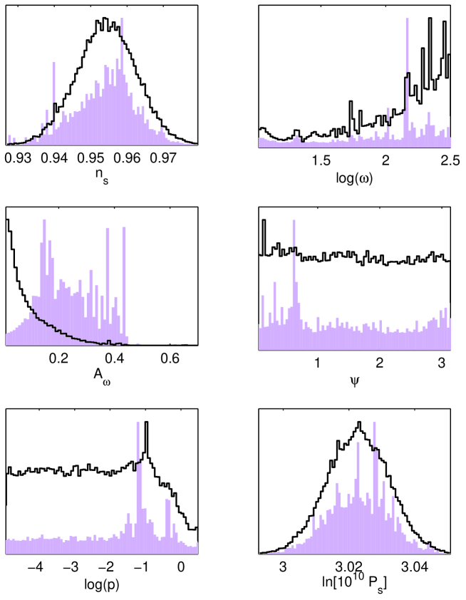
The posterior marginalised distributions given the third year WMAP data are plotted in figure 36. One still observes some particular frequencies improving the fit to the data while their weight on the marginalised probability remains negligible (see the $A_{\omega}$ posterior). The associated best fit value corresponds to $\chi^{2}=11242.7$, hence a $\Delta\chi^{2}\simeq-10$ with respect to a fiducial power law model, with however four additional parameters. This result is in agreement with the one found by the WMAP team [2]. However, it is important to stress that as soon as one consider non-logarithmic oscillations, the effect coming from modifying the pivot scale $k_{*}$ can not longer being viewed as a phase redefinition. In the present approach, we have not considered this effect and $k_{*}$ has been kept to its standard value $0.05\,\mathrm{Mpc}^{-1}$. In this respect, the posterior on $\log(p)$ leads to a two-sigma level upper bound

$$p<0.68\,,$$ (185)

in favour of small $p$ value, i.e. logarithmic-like superimposed oscillations.

6 Discussion and Conclusion

In this last section, we would like to briefly recap the results obtained in this article. In a first step, we have studied the compatibility of inflation with the WMAP3 CMB data using the slow-roll approximation. We have found that, at leading order, the first slow-roll parameter satisfies at $95\%$ of confidence

$$\epsilon_{1}<0.022\,.$$ (186)

These constraints implies an upper bound on the contribution of primordial gravitational waves, namely $r_{10}<0.21$ at $2\sigma$. This also leads to an upper bound on the energy scale of inflation $H/m_{\scriptscriptstyle{\mathrm{Pl}}}<1.3\times 10^{-5}$.

The WMAP3 data also constraint the second slow-roll parameter (at the $2\sigma$ level)

$$-0.02<\epsilon_{2}<0.09\,,\qquad-0.07<\epsilon_{2}<0.07\,,$$ (187)

the first result being derived with a Jeffrey’s prior on $\epsilon_{1}$ while the second is obtained with a uniform prior on $\epsilon_{1}$. We see that positive $\epsilon_{2}$, hence red spectral index, are slightly favoured although a scale-invariant power spectrum remains compatible with the data. At the second order in the slow-roll parameter a tendency for $\epsilon_{3}>0$ is observed but this is not statistically significant. Together with $\epsilon_{2}>0$, this would imply a negative scalar running.

Our second step has been to exactly integrate, using numerical methods, the inflationary power spectra for four fiducial models. The four models considered were the large field, small field, hybrid and running mass scenarios. For large field models $V(\phi)\propto\phi^{p}$, we have found the $2\sigma$ upper limit

$$p<3.1\,.$$ (188)

With regards to the subsequent reheating period, constraints on the reheating temperature can be found but only for the models that have an index $p$ such that they are already excluded. These constraints are therefore not of so much interest and are maybe just another indication that these models are now incompatible with the CMB data.

For small field models, the situation is slightly more complicated. A priori no constraint on $p$ and/or $\mu$ can be found given the WMAP3 data. But this statement is not completely prior independent. Indeed, if one assumes that $\mu/m_{\scriptscriptstyle{\mathrm{Pl}}}<100$, then the marginalised probability over $\mu$ is flat. But if one considers that $\mu/m_{\scriptscriptstyle{\mathrm{Pl}}}<10$, then the case $p=2$ is disfavoured. The situation is even more complicated because, if small values of $\mu/m_{\scriptscriptstyle{\mathrm{Pl}}}$ may appear to be appealing from a theoretical point of view, the scale $\mu$ should not be too small in order for the inflation energy scale $M$ to be larger than, say, the MeV. Another interesting issue related to the small field models is the reheating phase. These models are the only ones for which it is possible to say something on the reheat temperature given the WMAP3 data. The bounds are relatively weak since we find after marginalisation

$$T_{\mathrm{reh}}>2\,\mbox{TeV}\,,$$ (189)

at $95\%$ of confidence. Moreover, they are valid only for quite an extreme equation of state during reheating, namely $w_{\mathrm{reh}}\simeq-1/3$.

We have also studied the hybrid and running mass models. For those models, it is even more difficult to say something. Basically, hybrid models are disfavoured ($\Delta\chi^{2}=+5$) because of their blue spectrum while no prior independent constraint can be put on the running mass models because of the strong degeneracy among the parameters. But this class of models remain compatible with the CMB data.

The last section of the paper was devoted to the possible presence of superimposed oscillations in the power spectra. The marginalised probability is still centred on $|x|\sigma_{0}=0$, i.e. still compatible with no oscillations. At the $2\sigma$ level, one has obtained

$$|x|\sigma_{0}<0.38\,.$$ (190)

However, the likelihood is peaked at a non-vanishing value of $|x|\sigma_{0}$ corresponding to $\Delta\chi^{2}=-12$ for $3$ extra parameters. This apparent discrepancy is explained by the fact that the best fit occupies a small volume in the parameters space. One can nevertheless made the following two remarks. First, the overall statistical weight of the superimposed oscillations has increased in comparison with WMAP1 data and despite the disappearance of some of the cosmic variance outliers. One could have expected exactly the opposite. Secondly, we have also tested another functional shape for the superimposed oscillations and have shown that it does not improve the fit in the same manner, $\Delta\chi^{2}=-10$ for $4$ extra parameters. This suggests that the precise shape of the superimposed oscillations is relevant and that logarithmic oscillations are favoured. Notice, however, that the best fit solution, if interpreted in the trans-Planckian framework, suffers from a severe backreaction problem.

Let us conclude this article by a few words about the future. The flow of high accuracy data has not yet dried up and the forthcoming CMB experiments, as Planck [89], will provide us with even more accurate data which will help us to improve our constraints on the various inflationary scenarios. Using the slow-roll language, an exciting prospect would be to close the contour of the $\epsilon_{1}$ parameter. This would imply a detection of primordial gravitational waves and would open the possibility to test the consistency check $r_{10}\sim-5n_{\scriptscriptstyle{\mathrm{T}}}$, a smoking gun for slow-roll inflation. But even if this cannot be done in a close future, the example of small field models has taught us that this could also improve our knowledge of the reheating period. Indeed, we have seen that the constraint on $\ln R$ was directly linked to the constraint on the shape of the primordial power spectra. Shrinking the error bars on the tilt could therefore help us to put relevant limits on $T_{\mathrm{reh}}$, at least for the small field models but, maybe, also for the other class of inflationary scenarios. On the exact integration side, the method we have presented could be applied to more complicated models of inflation, especially to those transiently violating the slow-roll conditions or to the ones involving several interacting fields. Assuming only linear perturbation theory, such an approach directly leads to marginalised constraints on the fundamental parameters, as the ones involved in the inflaton potential and reheating. A natural extension would be the determination of the Bayesian evidence associated with each of the model tested [138, 56]. This would allow a statistical meaningful measure to prefer one inflationary model over the others.

References