An introduction to inflation and cosmological perturbation theory

Abstract

This article provides an introductory review of inflation and cosmological perturbation theory. I begin by motivating the need for an epoch of inflation during the early stages of the radiation dominated era, and describe how inflation is typically achieved using scalar fields. Then, after an overview of linear cosmological perturbation theory, I derive the equations governing the perturbations, and outline the generation of the scalar and the tensor perturbations during inflation. I illustrate that slow roll inflation naturally leads to an almost scale invariant spectrum of perturbations, a prediction that seems to be in remarkable agreement with the measurements of the anisotropies of the cosmic microwave background. I describe the constraints from the recent observations on some of the more popular models of inflation. I conclude with a brief discussion on the status and certain prospects of the inflationary paradigm.

I Introduction

I.1 A major drawback of the hot big bang model

The prevailing theory about the origin and the evolution of our universe is the so-called hot big bang model. The model is based on two crucial observations: the discovery of the expansion of the universe as characterized by the Hubble’s law, and the existence of an exceedingly isotropic and a perfectly thermal Cosmic Microwave Background (CMB) radiation. Since the energy density of radiation falls faster with the expansion than that of matter, these two observations immediately point to the fact that the universe has expanded from a hot and dense early phase, when radiation, rather than matter, was dominant. The transition to the more recent matter dominated epoch occurs when the radiation density falls sufficiently low that the photons cease to interact with matter. The CMB is nothing but the relic radiation which is reaching us today from this epoch of decoupling. While fairly isotropic, the CMB possesses small anisotropies (of about one part in $10^{5}$), and the observed pattern of the fluctuations in the CMB provides a direct snapshot of the universe at this epoch. The hot big bang model has been rather successful in predicting, say, the primordial abundances of the light elements in terms of a single parameter, viz. the baryon-to-photon ratio, and the value required to fit these observations matches the value that has been arrived at independently from the structure of the anisotropies in the CMB. Despite the success of the hot big bang model in explaining the results from different observations, the model has a serious drawback. Under the model, the CMB photons arriving at us today from sufficiently widely separated directions in the sky could not have interacted at the time of decoupling. Nevertheless, one finds that the temperature of the CMB photons reaching us from any two diametrically opposite directions hardly differ. (For a detailed description of the various successes and the few shortcomings of the hot big bang model, and the original references for the different points mentioned above, I would refer the reader to the following texts kolb-1990 ; linde-1990 ; liddle-1999 ; paddy-2002 ; dodelson-2003 ; mukhanov-2005 ; weinberg-2008 ; durrer-2008 .)

I.2 The scope and success of inflation

Inflation—which refers to a period of accelerated expansion during the early stages of the radiation dominated epoch—provides a satisfactory resolution to above-mentioned shortcoming of the hot big bang model. In fact, in addition to offering an elegant explanation for the extent of homogeneity and isotropy of the background universe, inflation also provides an attractive causal mechanism to generate the inhomogeneities superimposed upon it. The inflationary epoch amplifies the tiny quantum fluctuations present at the beginning of the epoch and converts them into classical perturbations which leave their imprints as anisotropies in the CMB. These anisotropies in turn act as seeds for the formation of the large scale structures that we observe at the present time as galaxies and clusters of galaxies. With the anisotropies in the CMB being measured to greater and greater precision, we have an unprecedented scope to test the predictions of inflation. As I shall discuss, the simplest models of inflation driven by a single, slowly rolling scalar field, generically predict a nearly scale invariant spectrum of primordial perturbations, which seems to be in excellent agreement with the recent observations of the CMB. (For a discussion on these different aspects of the inflationary paradigm, in addition to the texts kolb-1990 ; linde-1990 ; liddle-1999 ; paddy-2002 ; dodelson-2003 ; mukhanov-2005 ; weinberg-2008 ; durrer-2008 , see the following reviews kodama-1984 ; brandenberger-1985 ; mukhanov-1992 ; durrer-1994 ; lidsey-1997 ; lyth-1999 ; riotto-2002 ; kinney-2003 ; durrer-2004 ; martin-2004 ; giovannini-2005 ; bassett-2006 ; giovannini-2007 ; straumann-2006 ; kinney-2009 .)

I.3 The organization of this review

This article presents an introductory survey of inflation and linear cosmological perturbation theory, and it is organized as follows. In the next section, I shall describe the main shortcoming of the hot big bang model, viz. the horizon problem. In Sec. III, I shall outline how inflation helps to overcome the horizon problem, and illustrate how inflation can be driven with scalar fields. I shall also introduce the concept of slow roll inflation, and discuss the solutions to the background equations for a certain class of inflationary models in the slow roll approximation. In Sec. IV, I shall present an overview of linear perturbation theory. I shall explain the classification of the perturbations into scalars, vectors and tensors, and derive the equations governing these perturbations. I shall also discuss the behavior of the scalar perturbations in a particular limit. In Sec. V, after describing the generation of perturbations during inflation, I shall calculate the scalar and the tensor spectra that arise in power law as well as slow roll inflation. In Sec. VI, I shall discuss how such spectra compare with the recent observations, and point out the constraints on some of the more popular models of inflation. Finally, in Sec. VII, I shall conclude with a brief discussion on the status and some prospects of the inflationary paradigm.

I.4 Conventions and notations

Before I get down to brass tacks, let me list the various conventions and notations that I shall adopt. Unless I mention otherwise, I shall work in $(3+1)$-dimensions, and I shall adopt the metric signature of $(+,-,-,-)$. While Greek indices shall denote all the spacetime coordinates, the Latin indices shall refer to the spatial coordinates. I shall set $\hbar=c=1$, but shall display $G$ explicitly, and define the Planck mass to be $M_{{}_{\rm P}}=\left(8\,\pi\,G\right)^{-1/2}$. I shall express the various quantities in terms of either the cosmic time $t$ or the conformal time $\eta$, as is convenient. An overdot and an overprime shall denote differentiation with respect to the cosmic and the conformal time coordinates of the Friedmann metric that describes the expanding universe. It is useful to note here that, for any given function, say, $f$, ${\dot{f}}=(f^{\prime}/a)$ and ${\ddot{f}}=\left[\left(f^{\prime\prime}/a^{2}\right)-\left(f^{\prime}\,a^{\prime}/a^{3}\right)\right]$, where $a$ is the scale factor associated with the Friedmann metric. Lastly, since observations indicate that the universe has a rather small curvature, as it is usually done in the context of inflation, I shall work with the spatially flat Friedmann model.

I.5 A few words on the references

The different texts kolb-1990 ; linde-1990 ; liddle-1999 ; paddy-2002 ; dodelson-2003 ; mukhanov-2005 ; weinberg-2008 ; durrer-2008 and the variety of reviews kodama-1984 ; brandenberger-1985 ; mukhanov-1992 ; durrer-1994 ; lidsey-1997 ; lyth-1999 ; riotto-2002 ; kinney-2003 ; durrer-2004 ; martin-2004 ; giovannini-2005 ; bassett-2006 ; straumann-2006 ; giovannini-2007 ; kinney-2009 that I have already mentioned discuss the motivations for the inflationary scenario, the different models of inflation, the formulation of cosmological perturbation theory, and also how the various models compare with the recent observations. In what follows, I shall typically refer to one or more of these texts or reviews. I have also tried to refer to the original papers. However, I should stress that these references are often representative and not necessarily exhaustive.

II The horizon problem

Let me begin by describing the horizon problem in the hot big bang model. Consider a spatially flat, smooth, Friedmann universe described by line element

$${\rm d}s^{2}={\rm d}t^{2}-a^{2}(t)\;{\rm d}{\bf x}^{2}=a^{2}(\eta)\,\left({\rm d}\eta^{2}-{\rm d}{\bf x}^{2}\right),$$ (1)

where $t$ is the cosmic time, $a(t)$ is the scale factor, and $\eta=\int\,[{\rm d}t/a(t)]$ denotes the conformal time coordinate. In such a background, the horizon, viz. the size of a causally connected region, is defined as the physical radial distance travelled by a light ray from the big bang singularity at $t=0$ up to a given time $t$. The horizon can be expressed in terms of the scale factor $a(t)$ as follows mukhanov-2005 ; weinberg-2008 :

$$h(t)=a(t)\int\limits_{0}^{t}\frac{{\rm d}{\tilde{t}}}{a\left({\tilde{t}}\right)}.$$ (2)

Let me now compare the linear dimension of the forward and the backward light cones at the time of decoupling in the hot big bang model.

If one assumes that the universe was dominated by non-relativistic matter from the time of decoupling $t_{\rm dec}$ until today $t_{0}$, then the physical size of the region on the last scattering surface from which we receive the CMB is given by

$$\ell_{{}_{\rm B}}\left(t_{0},t_{\rm dec}\right)=a_{\rm dec}\,\int\limits_{t_{\rm dec}}^{t_{0}}\frac{{\rm d}{\tilde{t}}}{a\left({\tilde{t}}\right)}\simeq 3\,\left(t_{\rm dec}^{2}\,t_{0}\right)^{1/3},$$ (3)

where $a_{\rm dec}$ denotes the value of the scale factor at decoupling, and I have used the fact that $t_{0}\gg t_{\rm dec}$ in arriving at the final expression. On the other hand, if I assume that the universe was radiation dominated from the big bang until the epoch of decoupling, then the linear dimension of the horizon at decoupling turns out to be

$$\ell_{{}_{\rm F}}\left(t_{\rm dec},0\right)=a_{\rm dec}\,\int\limits_{0}^{t_{\rm dec}}\,\frac{{\rm d}{\tilde{t}}}{a\left({\tilde{t}}\right)}=\left(2\,t_{\rm dec}\right).$$ (4)

The ratio, say, $R$, of the linear dimensions of the backward and the forward light cones at decoupling then reduces to bassett-2006

$$R\equiv\left(\frac{\ell_{{}_{\rm B}}}{\ell_{{}_{\rm F}}}\right)=\left(\frac{3}{2}\right)\,\left(\frac{t_{0}}{t_{\rm dec}}\right)^{1/3}\simeq 70,$$ (5)

and the last equality follows from the observational fact that $t_{0}\simeq 10^{10}\;{\rm years}$, while $t_{\rm dec}\simeq 10^{5}\;{\rm years}$. In other words, the linear dimension of the backward light cone is about $70$ times larger than the forward light cone at decoupling. Despite this, the CMB turns out to be extraordinarily isotropic. This is the horizon problem.

There is another way of stating the horizon problem. Note that the physical wavelengths associated with the perturbations, say, $\lambda_{{}_{\rm P}}$, always grow as the scale factor, i.e. $\lambda_{{}_{\rm P}}\propto a$. In contrast, in a power law expansion of the form $a(t)\propto t^{q}$, the Hubble radius, viz. $d_{{}_{\rm H}}=H^{-1}=({\dot{a}}/a)^{-1}$, goes as $a^{1/q}$, so that we have $(\lambda_{{}_{\rm P}}/d_{{}_{\rm H}})\propto a^{[(q-1)/q]}$. This implies that, when $q<1$—a condition which applies to both the radiation and the matter dominated epochs—the physical wavelength grows faster than the corresponding Hubble radius as we go back in time kolb-1990 . In other words, the primordial perturbations need to be correlated on scales much larger than the Hubble radius at sufficiently early times in order to result in the anisotropies that we observe in the CMB. Consequently, within the hot big bang model, any mechanism that is invoked to generate the primordial fluctuations has to be intrinsically acausal.

III The inflationary scenario

Actually, apart from the horizon problem, there also exist a few other puzzles to which the hot big bang model is unable to provide a satisfactory solution. These other issues include, the extent to which the universe happens to be spatially flat today (to about one part in $10^{2}$), and the unacceptable density of relics that would have been formed when high energy symmetries were broken in the early universe, to name just two. Amongst all these issues, the horizon problem is arguably the most significant. Moreover, it so happens that, the inflationary solution to the horizon problem also aids in surmounting the other difficulties as well starobinsky-1979-1980 ; kazanas-1980 ; sato-1981 ; guth-1981 ; linde-1982 ; albrecht-1982 . For these reasons, I shall restrict my attention to the horizon problem. In the following sub-sections, after illustrating how inflation helps in overcoming the horizon problem, I shall outline how inflation is typically achieved with scalar fields.

III.1 Bringing the modes inside the Hubble radius

As I discussed above, length scales of cosmological interest today (say, $1\,\lesssim\lambda_{0}\lesssim 10^{4}\;{\rm Mpc}$), enter the Hubble radius either during the radiation or the matter dominated epochs, and are outside the Hubble radius at earlier times. If a causal mechanism is to be responsible for the origin of the inhomogeneities, then, clearly, these length scales should be inside the Hubble scales (i.e. $\lambda_{{}_{\rm P}}<d_{{}_{\rm H}}$) in the very early stages of the universe. This will be possible provided we have an epoch in the early universe during which $\lambda_{{}_{\rm P}}$ decreases faster than the Hubble radius as we go back in time, i.e. if we have dodelson-2003 ; kinney-2009

$$-\frac{{\rm d}}{{\rm d}t}\left(\frac{\lambda_{{}_{\rm P}}}{d_{{}_{\rm H}}}\right)<0,$$ (6)

which then leads to the condition that

$${\ddot{a}}>0.$$ (7)

In other words, the universe needs to undergo a phase of accelerated (inflationary) expansion during the early stages of the radiation dominated epoch if a physical mechanism is to account for the generation of the primordial fluctuations.

In order to illustrate these points, in Fig. 1, I have plotted ${\rm log}\;({\rm length})$, where ‘length’ denotes either the physical wavelength of a mode or the Hubble radius, against ${\rm log}\;a$, during inflation and the radiation dominated epochs kolb-1990 .

Figure 1: Evolution of the physical wavelength $\lambda_{\rm p}$ (in green) and the Hubble radius $d_{{}_{\rm H}}$ (in blue) has been plotted as a function of the scale factor $a$ on a logarithmic plot during the inflationary and the radiation dominated epochs. As discussed in the text, in such a plot, the slope of the Hubble length is much less than unity during inflation, a feature which allows to bring around the modes inside the Hubble radius at a suitably early time.

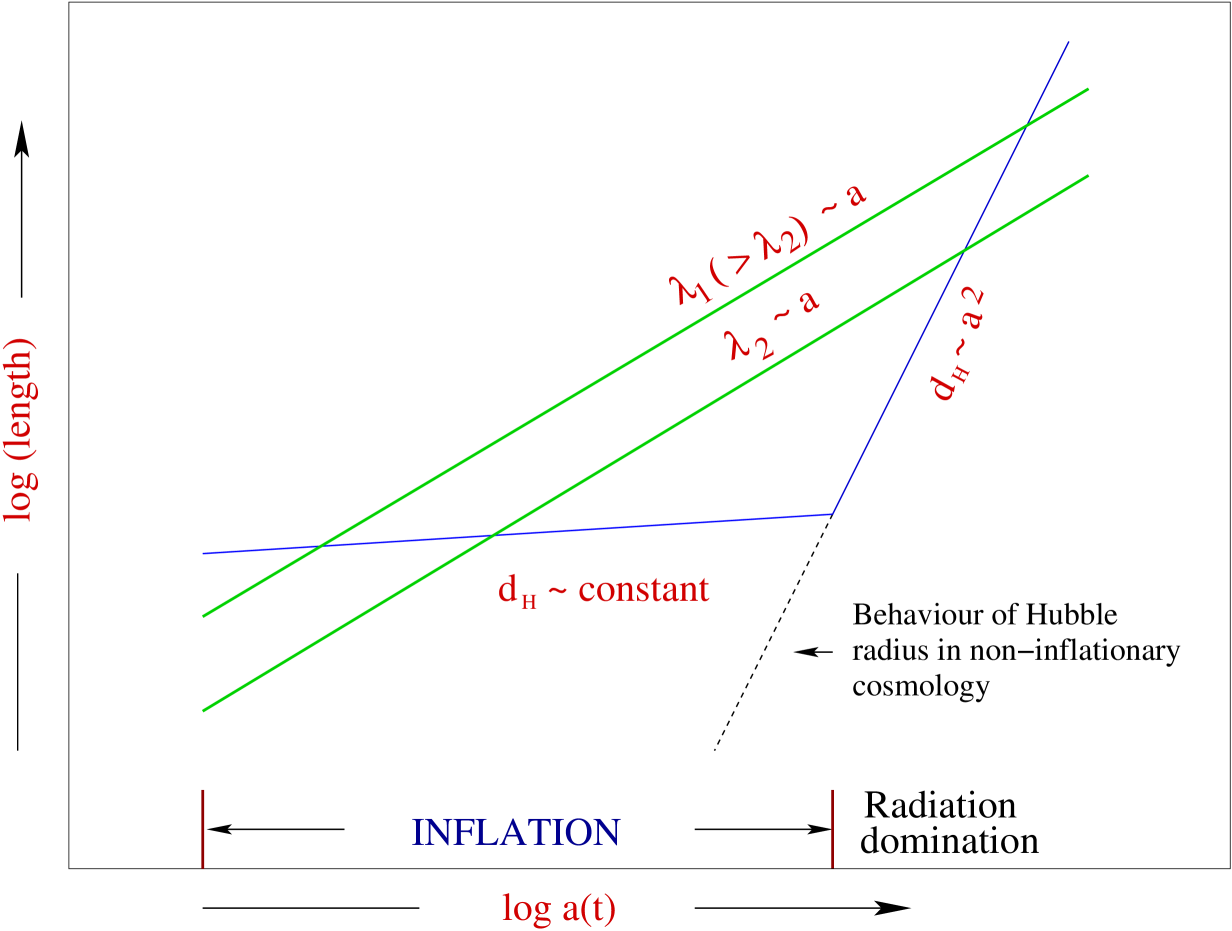
For convenience, I have chosen to describe inflation by the power law expansion $a\propto t^{q}$, with $q>1$. In such a situation, while $\lambda_{{}_{\rm P}}\propto a$ during all the epochs, the Hubble length $d_{{}_{\rm H}}$ behaves as $a^{1/q}$ and $a^{2}$ during inflation and the radiation dominated epochs. Evidently, all these quantities will be described by straight lines in the above plot. Whereas the straight lines describing the evolution of the physical wavelengths will have a unit slope, those describing the Hubble radius during the inflationary and the radiation dominated epochs will have a slope of much less than unity (say, for $q\gg 1$) and two, respectively. It is then clear from the figure that, as we go back in time, modes that leave the Hubble radius during the later epochs will not be inside the Hubble radius during the early stages of the universe unless we have a period of inflation.

III.2 How much inflation do we need?

Let us now try and understand as to how much inflation we shall require in order to ensure that the forward lightcone from the big bang to the epoch of decoupling is at least as large as the backward light cone from today to the epoch of decoupling, thereby resolving the horizon problem. For simplicity, let me assume that the universe undergoes exponential inflation, say, from time $t_{\rm i}$ to $t_{\rm f}$, during the early stages of the radiation dominated epoch. Let ${\sf H}$ be the constant Hubble scale during exponential inflation, and $A$ denote the extent by which the scale factor increases during the inflationary epoch. For $A\gg 1$, the dominant contribution to the size of the horizon at decoupling arises due to the rapid expansion during inflation, and it can be evaluated to be

$$\ell_{{}_{\rm I}}\left(t_{\rm dec},0\right)=a_{\rm dec}\,\int\limits_{0}^{t_{\rm dec}}\,\frac{{\rm d}{\tilde{t}}}{a\left({\tilde{t}}\right)}\simeq\left(\frac{a_{\rm dec}}{\sf H}\right)\,\left(\frac{t_{\rm dec}}{t_{\rm f}}\right)^{1/2}\,A,$$ (8)

where I have set $t_{\rm i}\simeq{\sf H}^{-1}$. In such a case, the ratio of the forward and the backward lightcones at the epoch of decoupling is given by paddy-2002

$$R_{{}_{\rm I}}\equiv\left(\frac{\ell_{{}_{\rm I}}}{\ell_{{}_{\rm B}}}\right)\simeq\left(\frac{A}{10^{26}}\right)$$ (9)

and, in arriving at the final number, I have chosen ${\sf H}\simeq 10^{13}\;{\rm GeV}$. Clearly, $R_{{}_{\rm I}}\simeq 1$, if $A\simeq 10^{26}$. Given the scale factor, the amount of expansion that has occurred from an initial time $t_{\rm i}$ to a time $t$ is usually expressed in terms of the number of $e$-folds defined as follows:

$$N=\int\limits_{t_{\rm i}}^{t}{\rm d}t\;H={\rm ln}\;\left(\frac{a(t)}{a_{\rm i}}\right).$$ (10)

Since ${\rm ln}\;A={\rm ln}\;(a_{\rm f}/a_{\rm i})\simeq 60$, it is often said that one requires about $60$ $e$-folds of inflation to overcome the horizon problem.

III.3 Driving inflation with scalar fields

If $\rho$ and $p$ denote the energy density and pressure of the smooth component of the matter field that is driving the expansion, then the Einstein’s equations corresponding to the line element (1) result in the following two Friedmann equations for the scale factor $a(t)$:

$$H^{2} = \left(\frac{8\,\pi\,G}{3}\right)\,{\rho},$$ (11a)

$$\left(\frac{\ddot{a}}{a}\right) = -\left(\frac{4\,\pi\,G}{3}\right)\,\left({\rho}+3\,p\right),$$ (11b)

where, as I had mentioned, $H=\left({\dot{a}}/a\right)$ is the Hubble parameter. It is clear from the second Friedmann equation that, for ${\ddot{a}}$ to be positive, we require that $\left({\rho}+3\,p\right)<0$. Neither ordinary matter (corresponding to $p=0$) nor radiation [which corresponds to $p=(\rho/3)$] satisfy this condition. In such a situation, we need to identify another form of matter to drive inflation.

Scalar fields, which are often encountered in various models of high energy physics, can easily help us achieve the necessary condition, thereby leading to inflation. Consider a canonical scalar field, say, $\phi$, described by the potential $V(\phi)$. Such a scalar field is governed by the action

$$S[\phi]=\int\!{\rm d}^{4}x\;\sqrt{-g}\,\left[\left(\frac{1}{2}\right)\,\left({\partial}_{\mu}\phi\;{\partial}^{\mu}\phi\right)-V(\phi)\right],$$ (12)

with the associated stress-energy tensor being given by

$$T^{\mu}_{\nu}={\partial}^{\mu}\phi\;{\partial}_{\nu}\phi-\delta^{\mu}_{\nu}\,\left[\left(\frac{1}{2}\right)\;\left({\partial}_{\lambda}\phi\;{\partial}^{\lambda}\phi\right)-V(\phi)\right].$$ (13)

The symmetries of the Friedmann background—viz. homogeneity and isotropy—imply that the scalar field will depend only on time and, hence, the resulting stress-energy tensor will be diagonal. Therefore, the energy density $\rho$ and the pressure $p$ associated with the scalar field simplify to

$$T^{0}_{0} = \rho=\left[\left(\frac{{\dot{\phi}}^{2}}{2}\right)+V(\phi)\right],$$ (14a)

$$T^{i}_{j} = -p\;\delta^{i}_{j}=-\left[\left(\frac{{\dot{\phi}}^{2}}{2}\right)-V(\phi)\right]\,\delta^{i}_{j}.$$ (14b)

Moreover, from the action (12), one can arrive at the following equation of motion for the scalar field $\phi$ in the Friedmann universe:

$${\ddot{\phi}}+3\,H\,{\dot{\phi}}+V_{\phi}=0,$$ (15)

where $V_{\phi}=({\rm d}V/{\rm d}\phi)$. From the above expressions for $\rho$ and $p$, one finds that the condition for inflation, viz. $(\rho+3\,p)<0$, reduces to

$${\dot{\phi}}^{2}<V(\phi).$$ (16)

In other words, inflation can be achieved if the potential energy of the scalar field dominates its kinetic energy.

Given a $V(\phi)$ that is motivated by a high energy model, the first Friedmann equation (11a) and the equation (15) that governs the evolution of the scalar field have to be consistently solved for the scale factor and the scalar field, with suitable initial conditions. But, using the expressions (14) for the energy density and the pressure associated with the scalar field, the Friedmann equations (11) can be rewritten as

$$H^{2} = \left(\frac{1}{3\,M_{{}_{\rm P}}^{2}}\right)\;\left[\left(\frac{{\dot{\phi}}^{2}}{2}\right)+V(\phi)\right],$$ (17a)

$${\dot{H}} = -\left(\frac{1}{2\,M_{{}_{\rm P}}^{2}}\right)\,{\dot{\phi}}^{2},$$ (17b)

where, for convenience, I have set $(8\,\pi\,G)=M_{{}_{\rm P}}^{-2}$, as I had defined earlier. These two equations can then be combined to express the scalar field and the potential parametrically in terms of the cosmic time $t$ as follows paddy-2002 :

$$\phi(t) = \sqrt{2}\;M_{{}_{\rm P}}\,\int\!{\rm d}t\;\sqrt{\left(-{\dot{H}}\right)},$$ (18a)

$$V(t) = M_{{}_{\rm P}}^{2}\;\;\left(3\,H^{2}+{\dot{H}}\right).$$ (18b)

If we know the scale factor $a(t)$, these two equations allow us to ‘reverse engineer’ the potential from which such a scale factor can arise! Using this procedure, I shall now ‘reconstruct’ the potentials of two commonly considered models of inflation.

Consider the power law expansion

$$a(t)=a_{1}\,t^{q}$$ (19)

with $q>1$ corresponding to inflation, and $a_{1}$ being an arbitrary constant. On substituting this scale factor in equation (18a) and, upon integration, one can immediately show that the scalar field evolves as

$$\left(\frac{\phi(t)}{M_{{}_{\rm P}}}\right)=\sqrt{(2\,q)}\;\;{\rm ln}\,\left[\sqrt{\left(\frac{V_{0}}{(3\,q-1)\,q}\right)}\,\left(\frac{t}{M_{{}_{\rm P}}}\right)\right],$$ (20)

where $V_{0}$ is a constant of integration. The potential that leads to such a behavior can then be obtained using equation (18b), and the above expressions for $a(t)$ and $\phi(t)$. It is found to be lucchin-1985

$$V(\phi)=V_{0}\,\exp\,-\left[\sqrt{\frac{2}{q}}\,\left(\frac{\phi}{M_{{}_{\rm P}}}\right)\right].$$ (21)

In a similar fashion, it is straightforward to establish that the potential

$$V(\phi)=\left(3\,\alpha^{2}\,\beta^{2}\,\Gamma^{\kappa}\,M_{{}_{\rm P}}^{2}\right)\!\left[1-\left(\frac{\kappa^{2}}{6}\right)\!\left(\frac{M_{{}_{\rm P}}}{\phi}\right)^{2}\right]\!\left(\frac{\phi}{M_{{}_{\rm P}}}\right)^{-\kappa}\!\!,$$ (22)

where $\Gamma=\sqrt{(2\,\alpha\,\kappa)}$ and $\kappa=[4\,(1-\beta)/\beta]$, leads to the following behavior for $a(t)$:

$$a(t)=a_{1}\,\exp\,\left(\alpha\,t^{\beta}\right)$$ (23)

with $\alpha>0$ and $0<\beta<1$, and $a_{1}$ is again some arbitrary constant. Since this scale factor grows faster than power law inflation, but slower than exponential expansion, it is referred to as intermediate inflation barrow-1990 ; muslimov-1990 .

III.4 Slow roll inflation

The condition (16) that the potential energy of the inflaton dominates the kinetic energy is necessary for inflation to take place. However, inflation is guaranteed, if the field rolls slowly down the potential such that

$${\dot{\phi}}^{2}\ll V(\phi).$$ (24)

Moreover, it can be ensured that the field is slowly rolling for a sufficiently long time (to achieve the required $60$ or so $e$-folds of inflation), provided

$${\ddot{\phi}}\ll\left(3\,H\,{\dot{\phi}}\right).$$ (25)

These two conditions lead to the slow roll approximation steinhardt-1984 ; salopek-1990 ; liddle-1992 , which, as we shall see, allows one to construct analytical solutions, both for the background and the perturbations. The approximation is usually described in terms of what are referred to as the slow roll parameters. Two types of slow roll parameters—the potential slow roll parameters and the Hubble slow roll parameters—are often considered in the literature. I shall describe these two sets of parameters below, and discuss the solutions for the inflaton and the scale factor for a particular class of potentials in the slow roll approximation.

III.4.1 The potential slow roll parameters

When provided with a potential $V(\phi)$, the potential slow roll approximation corresponds to requiring the following two dimensionless parameters steinhardt-1984 ; salopek-1990 ; liddle-1992 :

$$\epsilon_{{}_{\rm V}}=\left(\!\frac{M_{{}_{\rm P}}^{2}}{2}\!\right)\,\left(\frac{V_{\phi}}{V}\right)^{2}\quad{\rm and}\quad\eta_{{}_{\rm V}}=M_{{}_{\rm P}}^{2}\,\left(\frac{V_{\phi\phi}}{V}\right),$$ (26)

where $V_{\phi\phi}\equiv\left({\rm d}^{2}V/{\rm d}\phi^{2}\right)$, to be small when compared to unity. The two quantities $\epsilon_{{}_{\rm V}}$ and $\eta_{{}_{\rm V}}$ are referred to as the Potential Slow Roll (PSR) parameters. It is straightforward to show that neglecting the kinetic energy term $({\dot{\phi}}^{2}/2)$ in the Friedmann equation (17a) and the acceleration term ${\ddot{\phi}}$ in the equation of motion (15) for the scalar field are equivalent to the smallness of these parameters. However, it should be emphasized that the converse is not true. The smallness of the PSR parameters is only a necessary condition, and it is not sufficient to ensure that these terms can indeed be ignored. The reason being that the PSR parameters only restrict the form of the potential, and not the dynamics of the solutions. Even if $\epsilon_{{}_{\rm V}}$ and $\eta_{{}_{\rm V}}$ are small, there is no assurance that inflation will take place since the value of $\dot{\phi}$ can be as large as possible. Therefore, in addition to the two PSR parameters being small, the slow roll approximation actually requires the additional condition that the scalar field is moving slowly along the attractor solution determined by the equation: $(3\,H\,{\dot{\phi}})=-V_{\phi}$ (for a detailed discussion on this point, see Ref. liddle-1994 ).

In spite of this shortcoming, the PSR parameters often prove to be very handy. For instance, given a potential, they immediately allow us to determine the domains and the parameters of the potential that can lead to inflation. I shall now discuss two examples to illustrate the utility of these parameters. Consider potentials of the form linde-1983

$$V(\phi)=\left(V_{0}\,\phi^{n}\right),$$ (27)

where $V_{0}$ is a constant and $n>0$. Let us restrict ourselves to the region $\phi>0$ wherein $V(\phi)$ is positive for all $n$. It is straightforward to show that the slow roll conditions [viz. $(\epsilon_{{}_{\rm V}},\eta_{{}_{\rm V}})\ll 1$] are satisfied when $\phi$ is much greater than $M_{{}_{\rm P}}$. Since inflation occurs for such large values of the field, these potentials are often classified as ‘large field’ models bassett-2006 . Now, consider the following potential which describes the pseudo-Nambu-Goldstone Boson

$$V(\phi)=\Lambda\,\left[1+{\rm cos}\,\left(\phi/f\right)\right],$$ (28)

where $\Lambda$ and $f$ are constants that characterize the depth and the width of the potential. This potential ‘naturally’ leads to inflation for values of the field that are small when compared to the Planck scale freese-1990 . Hence, such models are usually referred to as ‘small field’ models.

III.4.2 The Hubble slow roll parameters

The Hubble Slow Roll (HSR) parameters turn out to be a better choice to describe the slow roll approximation than the PSR parameters since they do not require any additional conditions to be satisfied for the approximation to be valid. The HSR parameters are called so, since they are defined in terms of the Hubble parameter $H$, which is treated as a function of the scalar field $\phi$ salopek-1990 . In such a case, we can write Eq. (17) as

$${\dot{\phi}}=-\left(2\,M_{{}_{\rm P}}^{2}\right)\,H_{\phi},$$ (29)

where $H_{\phi}\equiv({\rm d}H/{\rm d}\phi)$. This expression can then be used to rewrite the first Friedmann equation (17a) as follows:

$$H_{\phi}^{2}-\left(\frac{3\,H^{2}}{2\,M_{{}_{\rm P}}^{2}}\right)=-\left(\frac{V}{2\,M_{{}_{\rm P}}^{4}}\right),$$ (30)

a relation that is referred to as the Hamilton-Jacobi formulation of inflation salopek-1990 .

Taking $H(\phi)$ to be the primary quantity, the dimensionless HSR parameters $\epsilon_{{}_{\rm H}}$ and $\delta_{{}_{\rm H}}$ are defined as follows liddle-1994 :

$$\epsilon_{{}_{\rm H}}=\left(2\,M_{{}_{\rm P}}^{2}\right)\,\left(\frac{H_{\phi}}{H}\right)^{2}\quad{\rm and}\quad\eta_{{}_{\rm H}}=\left(2\,M_{{}_{\rm P}}^{2}\right)\,\left(\frac{H_{\phi\phi}}{H}\right),$$ (31)

where $H_{\phi\phi}\equiv\left({{\rm d}}^{2}H/{\rm d}\phi^{2}\right)$. On using Eqs. (15), (29) and (30), these two parameters can be written as

$$\epsilon_{{}_{\rm H}} = \left(\frac{3\,{\dot{\phi}}^{2}}{2\,\rho}\right)=-\left(\frac{\dot{H}}{H^{2}}\right),$$ (32a)

$$\delta_{{}_{\rm H}} = -\left(\frac{\ddot{\phi}}{H{\dot{\phi}}}\right)=\epsilon_{{}_{\rm H}}-\left(\frac{\dot{\epsilon}_{{}_{\rm H}}}{2\,H\,\epsilon_{{}_{\rm H}}}\right),$$ (32b)

where $\rho$ is the energy density associated with the scalar field. The following points are clear from these expressions. Firstly, $\epsilon_{{}_{\rm H}}\ll 1$ is precisely the condition required for neglecting the kinetic energy term in the total energy of the scalar field. Secondly, the limit $\delta_{{}_{\rm H}}\ll 1$ corresponds to the situation wherein the acceleration term of the scalar field can be ignored in Eq. (15) when compared to the term involving the velocity. Finally, the inflationary condition ${\ddot{a}}>0$ exactly corresponds to $\epsilon_{{}_{\rm H}}<1$.

It should again be emphasized that, since the smallness of the HSR parameters ensure that ${\dot{\phi}}$ is small, the HSR approximation implies the PSR approximation. But, the converse does not hold without assuming the constraint that the inflaton is already on the attractor liddle-1994 .

III.4.3 Solutions in the slow roll approximation

Note that the equation of motion of the scalar field (15) and the first Friedmann equation (17a) can be written in terms of the two HSR parameters as

$$H^{2}\,\left[1-\left(\frac{\epsilon_{{}_{\rm H}}}{3}\right)\right] = \left(\frac{V}{3\,M_{{}_{\rm P}}^{2}}\right),$$ (33a)

$$\left(3\,H\,{\dot{\phi}}\right)\;\left[1-\left(\frac{\delta_{{}_{\rm H}}}{3}\right)\right] = -V_{\phi}.$$ (33b)

The slow roll approximation corresponds to the situation wherein the HSR parameters $\epsilon_{{}_{\rm H}}$ and $\delta_{{}_{\rm H}}$ satisfy the following conditions:

$$\epsilon_{{}_{\rm H}}\ll 1,\quad\delta_{{}_{\rm H}}\ll 1,\quad{\rm and}\quad\mathcal{O}\left[\epsilon_{{}_{\rm H}}^{2},\delta_{{}_{\rm H}}^{2},\left(\epsilon_{{}_{\rm H}}\delta_{{}_{\rm H}}\right)\right]\ll\epsilon_{{}_{\rm H}}.$$ (34)

At the leading order in the slow roll approximation, the equations (33) above reduce to

$$H^{2}\simeq\left(\frac{V}{3\,M_{{}_{\rm P}}^{2}}\right)\quad{\rm and}\quad\left(3\,H\,{\dot{\phi}}\right)\simeq-V_{\phi}.$$ (35)

Being first order differential equations, given a potential, these equations can be easily integrated to obtain the solutions to the scale factor and the scalar field in the slow roll limit. Let me now discuss the solutions in this limit to the large field models (27) that I had considered earlier.

For the potential (27), when $n\neq 4$, in the slow roll limit, the solution to the scalar field is given by durrer-2008 ; martin-2004

$$\phi^{[(4-n)/2]}(t)\simeq\phi^{[(4-n)/2]}_{\rm i}+\sqrt{\frac{V_{0}}{3}}\left[\frac{n\,(n-4)}{2}\right]M_{{}_{\rm P}}\,(t-t_{\rm i}),$$ (36)

whereas, when $n=4$, one finds that

$$\phi(t)\simeq\phi_{\rm i}\;\exp-\left[\sqrt{\left(V_{0}/3\right)}\;\left(4\,M_{{}_{\rm P}}\right)\,(t-t_{\rm i})\right]$$ (37)

and, in both these solutions, $\phi_{\rm i}$ is a constant that denotes the value of the scalar field at some initial time $t_{\rm i}$. For all $n$, the scale factor can be expressed in terms of these solutions for the scalar field as follows:

$$a(t)\simeq a_{\rm i}\;\exp-\left[\left(\frac{1}{2\,n\,M_{{}_{\rm P}}^{2}}\right)\,\left(\phi^{2}(t)-\phi^{2}_{\rm i}\right)\right]$$ (38)

with $a_{\rm i}$ being the value of the scalar factor at $t_{\rm i}$. It is also useful to note that, in the slow roll limit, the two equations (35) allow us to express the number of $e$-folds from $t_{\rm i}$ to $t$ during inflation as

$$N={\rm ln}\,\left(\frac{a}{a_{\rm i}}\right)=\int\limits_{t_{\rm i}}^{t}{\rm d}t\,H\simeq-\left(\frac{1}{M_{{}_{\rm P}}^{2}}\right)\,\int\limits_{\phi_{\rm i}}^{\phi}{\rm d}\phi\,\left(\frac{V}{V_{\phi}}\right),$$ (39)

where the upper limit $\phi$ is the value of the scalar field at the time $t$. In terms of $e$-folds, for the large field models, the scalar field and the Hubble parameter are given by

$$\!\!\!\!\!\!\!\!\!\!\!\!\!\!\!\!\phi^{2}(N) \simeq \left[\phi_{\rm i}^{2}-\left(2\,M_{{}_{\rm P}}^{2}\,n\right)\;N\right],\qquad\qquad$$ (40a)

$$\!\!\!\!\!\!\!\!\!\!\!\!\!\!\!\!H^{2}(N) \simeq \left(\!\frac{V_{0}\,M_{{}_{\rm P}}^{(n-2)}}{3}\!\right)\left[\left(\!\frac{\phi_{\rm i}}{M_{{}_{\rm P}}}\!\right)^{2}-\left(2\,n\,N\right)\right]^{(n/2)}\!\!\!\!\!\!\!\!\!.$$ (40b)

IV Essential linear, cosmological perturbation theory

Though the inflationary scenario was originally proposed to resolve the different puzzles related to the smooth background, it was soon realized that it also offers a simple mechanism to generate the primordial perturbations. Before I turn to demonstrating how inflation produces these inhomogeneities, I shall provide an overview of essential cosmological perturbation theory. (As I had mentioned, I will restrict myself to linear perturbations.) In what follows, after a discussion on the classification of the perturbations into scalars, vectors and tensors, I shall derive the equations governing these perturbations. Since the scalar perturbations are primarily responsible for the anisotropies in the CMB and the formation of structures, I shall also briefly highlight the evolution of these perturbations at super-Hubble scales during the radiation and the matter dominated epochs.

IV.1 Classification of the perturbations

CMB observations indicate that the anisotropies at the epoch of decoupling are rather small (one part in $10^{5}$, as I had mentioned). If so, the amplitude of the deviations from homogeneity will be even smaller at earlier epochs. This suggests that the generation and the evolution of the perturbations (until structures begin to form late in the matter dominated epoch), can be studied using linear perturbation theory.

In a Friedmann background, the metric perturbations can be decomposed according to their behavior under local rotation of the spatial coordinates on hypersurfaces of constant time. This property leads to the classification of the perturbations as scalars, vectors and tensors bardeen-1980 ; stewart-1990 . Scalar perturbations remain invariant under rotations (and, hence, can be said to have zero spin). As we shall see, these are the principal perturbations that are responsible for the anisotropies and the inhomogeneities in the universe. Vector and tensor perturbations—as their names indicate—transform as vectors and tensors do under rotations (and, as a result, have spins of unity and two, respectively). The vector perturbations are generated by rotational velocity fields and, therefore, are also referred to as the vorticity modes. Finally, the tensor perturbations describe gravitational waves, and it is important to note that they can exist even in the absence of sources grishchuk-1974 ; starobinsky-1979 .

IV.1.1 The number of independent scalar, vector and tensor degrees of freedom

Let us now carry out the exercise of counting the number of degrees of freedom associated with these different types of perturbations riotto-2002 . To highlight the counting procedure, in this sub-section, I shall, in fact, work in arbitrary spacetime dimensions. In $(D+1)$-dimensions, the metric tensor, being symmetric, has $[(D+1)\,(D+2)/2]$ degrees of freedom. However, not all of these degrees are independent since there exist $(D+1)$ degrees of freedom associated with the coordinate transformations. If we eliminate these degrees, we are left with a total of $[D\,(D+1)/2]$ independent degrees of freedom describing the metric perturbations. These degrees of freedom contain the scalar, the vector, and the tensor perturbations.

Let $\delta g_{\mu\nu}$ denote the metric perturbations in the Friedmann universe. The perturbed metric can be split as follows:

$$\delta g_{\mu\nu}=\left(\delta g_{00},\delta g_{0i},\delta g_{ij}\right).$$ (41)

Since it contains no running index, evidently, the perturbation $\delta g_{00}={\cal A}$, say, is a scalar. As is well known, one can always decompose a vector into a gradient of a scalar and a vector that is divergence free. Hence, we can write $\delta g_{0i}$ as

$$\delta g_{0i}=\left({\nabla}_{i}\,{\cal B}+{\cal S}_{i}\right),$$ (42)

where ${\cal B}$ is a scalar, while ${\cal S}_{i}$ is a vector that is divergence free, i.e. $\left({\nabla}_{i}\,{\cal S}^{i}\right)=0$. A similar decomposition can be carried for the quantity $\delta g_{ij}$ by essentially repeating the above analysis on each of the two indices. Therefore, the quantity $\delta g_{ij}$ can be decomposed as

$$\delta g_{ij}\!\! = \!\!\psi\;\delta_{ij}+\left({\nabla}_{i}\,{\cal F}_{j}+{\nabla}_{j}\,{\cal F}_{i}\right)$$ (43)

$$\qquad\,+\left[\left(\frac{1}{2}\right)\left({\nabla}_{i}\,{\nabla}_{j}+{\nabla}_{j}\,{\nabla}_{i}\right)-\left(\frac{1}{3}\right)\delta_{ij}\,{\nabla}^{2}\right]{\cal E}$$

$$\qquad\;+\,{\cal H}_{ij},$$

where $\psi$ and ${\cal E}$ are scalar functions, ${\cal F}_{i}$—like ${\cal S}_{i}$ above—is a divergence free vector, and ${\cal H}_{ij}$ is a symmetric, traceless and transverse tensor that satisfies the conditions ${\cal H}^{i}_{i}=0$ and $\left(\nabla_{i}\,{\cal H}^{ij}\right)=0$. Let me again count the degrees of freedom of the perturbed metric tensor through the various functions I have introduced. To describe $\delta g_{\mu\nu}$, we require the scalars ${\cal A}$, ${\cal B}$, $\psi$ and ${\cal E}$, amounting to four degrees of freedom. We also need the two divergence free spatial vectors ${\cal S}_{i}$ and ${\cal F}_{i}$ that add up to $[2\,(D-1)]$ degrees. Moreover, after we impose the traceless and transverse conditions, the tensor ${\cal H}_{ij}$ has

$$\left[\frac{D\,(D+1)}{2}\right]-(D+1)=\left[\frac{(D+1)\,(D-2)}{2}\right]$$ (44)

degrees of freedom. Upon adding all these scalar, vector and tensor degrees, I obtain

$$4+2\,(D-1)+\left[\frac{(D+1)\,(D-2)}{2}\right]\!=\!\left[\frac{(D+1)\,(D+2)}{2}\right]$$ (45)

which, as I discussed above, are the total number of degrees of freedom associated with the perturbed metric in $(D+1)$-dimensions.

In the same fashion, let me decompose the degrees of freedom associated with the coordinate transformations. In a Friedmann background, the $(D+1)$ coordinate transformations that relate different coordinate systems that describe the perturbed metric can be expressed in terms of scalars, say, $\delta t$ and $\delta x$, as follows:

$$t\to\left(t+\delta t\right)\quad{\rm and}\quad x^{i}\to\left[x^{i}+{\nabla}^{i}\,(\delta x)\right].$$ (46)

Similarly, one can construct coordinate transformations in terms of a divergence free vector, say, $\delta x^{i}$, as

$$t\to t\quad{\rm and}\quad x^{i}\to\left(x^{i}+\delta x^{i}\right).$$ (47)

(It should be emphasized that these coordinate transformations are of a particular form, and are not completely arbitrary. The form of these transformations is dictated by the fact that the difference between the coordinates are determined by the amplitude of the perturbations. In other words, it is a gauge transformation. I shall somewhat elaborate on this point below.) There is no further coordinate degrees of freedom associated with the tensor perturbations. The two scalar quantities $\delta t$ and $\delta x$, and the divergence free vector $\delta x^{i}$, constitute the $[2+(D-1)]=(D+1)$ degrees of freedom associated with the coordinate transformations.

Let me now subtract the coordinate degrees of freedom from the total degrees to arrive at the independent number of scalar, vector and tensor degrees of freedom. Four scalar functions, viz. $({\cal A},{\cal B},\psi,{\cal E})$, were required to describe the perturbed metric tensor $\delta g_{\mu\nu}$. But, there also exist two scalar degrees of freedom associated with one’s choice of coordinates, i.e. $\delta t$ and $\delta x$. Hence, the actual number of independent scalar degrees of freedom is $(4-2)=2$. And, it is useful to notice that this is true in arbitrary spacetime dimensions. I had needed two divergence free vector functions, ${\cal S}_{i}$ and ${\cal F}_{i}$, amounting to a total of $[2\,(D-1)]$ degrees of freedom, to describe the perturbed metric tensor. If we subtract the $(D-1)$ vector degrees of freedom corresponding to the coordinate transformations that can be achieved through $\delta x^{i}$ from this number, one is left with $[2\,(D-1)]-(D-1)=(D-1)$ true vector degrees of freedom. As I have already pointed out, the tensor perturbations contain $[(D+1)\,(D-2)/2]$ independent degrees of freedom. Upon adding these, I obtain that

$$2+(D-1)+\left[\frac{(D+1)\,(D-2)}{2}\right]=\left[\frac{D\,(D+1)}{2}\right]$$ (48)

which is the total number of independent degrees of freedom describing the perturbed metric tensor.

Note that, in the $(3+1)$-dimensional case of our interest, there exists two each of the scalar, the vector and the tensor degrees of freedom.

IV.1.2 The decomposition theorem

I have focused above on decomposing the perturbed metric tensor into the different types of perturbations. Let me now discuss the equivalent classification of the source of the metric perturbations, viz. the stress-energy tensor. Since the stress-energy tensor is a symmetric two tensor just as the metric tensor is, the perturbed stress-energy tensor can also be classified as the scalar, the vector and the tensor components. For instance, while the perturbed inflaton and perfect fluids—such as radiation and matter—are scalar sources, velocity fields with vorticity are, evidently, vector sources. Anisotropic stresses, when the possible scalar and vector contributions have been eliminated, constitute a tensor source.

Given the perturbed metric tensor $\delta g_{\mu\nu}$, the corresponding Einstein tensor, say, $\delta G_{\mu\nu}$, can immediately be calculated at the same order in the perturbations. The Einstein equations that relate the perturbed Einstein tensor to the perturbed stress-energy tensor, say, $\delta T_{\mu\nu}$, will then lead to the equations governing the perturbations. According to the decomposition theorem weinberg-2008 ; kodama-1984 , which I shall use without proof, at the linear order in the perturbations, the scalar, the vector and the tensor perturbations decouple and, hence, they can be analyzed separately. In other words, each type of metric perturbation is affected by only the same type of source. Therefore, the three types of perturbations can be studied independently of each other.

IV.1.3 Gauges

The Friedmann line element (1) describes the expanding universe in the frame of a comoving observer. The comoving observer is special since, it is with respect to such an observer that the universe appears homogeneous and isotropic. However, there is no such uniquely preferred frame of reference in the presence of perturbations. A variety of coordinate choices are possible, with the only requirement being that the metric and the coordinates reduce to the standard Friedmann line element in the limit when the perturbations vanish. As a result, the difference between the various coordinates have the same amplitude as the perturbations themselves. A particular choice of coordinates is called a gauge. If one changes the coordinate system, one would obtain another metric, i.e. a different gauge. The transformation from one gauge to another [such as Eqs. (46) and (47)] is referred to as a gauge transformation. There exists two approaches to studying the evolution of the perturbations. Either one constructs gauge invariant quantities, or chooses a particular gauge and work in the specific gauge throughout. Being simpler and more wieldy, I shall adopt the latter approach.

IV.2 Scalar perturbations

I shall now turn to deriving the equations of motion governing the three different types of perturbations. Let me first consider the case of the scalar perturbations.

IV.2.1 The longitudinal gauge and the perturbed Einstein tensor

As I mentioned above, I shall work in a particular gauge to describe the various perturbations. A convenient gauge to describe the scalar perturbations is the longitudinal gauge. If we take into account the scalar perturbations to the background metric (1), then, in this gauge, the Friedmann line element is given by

$${\rm d}s^{2}=\left(1+2\,\Phi\right)\,{\rm d}t^{2}-a^{2}(t)\;\left(1-2\,\Psi\right)\,{\rm d}{\bf x}^{2},$$ (49)

where $\Phi$ and $\Psi$ are the two independent functions that describe the perturbations. (Note that this choice of gauge corresponds to ${\cal A}\propto\Phi$, $\psi\propto\Psi$ and ${\cal B}={\cal E}=0$.) At the linear order in the perturbations, the components of the perturbed Einstein tensor, viz. $\delta G^{\mu}_{\nu}$, corresponding to the line element (49) above can be evaluated to be bassett-2006

$$\delta G_{0}^{0} = -6\,H\,\left({\dot{\Psi}}+H\,\Phi\right)+\left(\frac{2}{a^{2}}\right)\,{\nabla}^{2}\Psi,$$ (50a)

$$\delta G^{0}_{i} = 2\;{\nabla}_{i}\left({\dot{\Psi}}+H\,\Phi\right),$$ (50b)

$$\delta G^{i}_{j} = -2\;\biggl{[}{\ddot{\Psi}}+H\,\left(3\,{\dot{\Psi}}+{\dot{\Phi}}\right)$$ (50c)

$$\qquad\quad+\left(2\,{\dot{H}}+3\,H^{2}\right)\,\Phi+\left(\frac{1}{a^{2}}\right)\,{\nabla}^{2}{\cal D}\biggr{]}\;\delta^{i}_{j}$$

$$\qquad\quad+\left(\frac{1}{a^{2}}\right)\,{\nabla}^{i}\,{\nabla}_{j}{\cal D}.$$

where ${\cal D}=\left(\Phi-\Psi\right)$.

IV.2.2 Equations of motion

The only sources of perturbations that I shall consider in this review will be scalar fields and perfect fluids. As I shall illustrate in the next section, scalar fields do not possess any anisotropic stress at the linear order in the perturbations. I shall assume that the perfect fluids that I consider do not contain any anisotropic stresses either. Under these conditions, the perturbed stress-energy tensor associated with such sources can be expressed as follows:

$$\delta T^{0}_{0}=\delta\rho,\quad\delta T^{0}_{i}=\left({\nabla}_{i}\,\delta\sigma\right)\quad{\rm and}\quad\delta T^{i}_{j}=-\delta p\;\delta^{i}_{j},$$ (51)

where the quantities $\delta\rho$, $\delta\sigma$, and $\delta p$ are the scalar quantities that denote the perturbations in the energy density, the momentum flux, and the pressure, respectively. The first order Einstein’s equations, viz. $\delta G^{\mu}_{\nu}=\left(8\,\pi\,G\right)\,\delta T^{\mu}_{\nu}$, then lead to the required set of equations governing the perturbations. It is clear from the form of $\delta G^{i}_{j}$ above that, in the absence of anisotropic stresses, the corresponding Einstein equation leads to: $\Phi=\Psi$. In such a case, the remaining three Einstein equations simplify to bassett-2006

$$\!\!\!\!\!\!\!\!\!\!\!\!-3\,H\,\left({\dot{\Phi}}+H\,\Phi\right)+\left(\!\frac{1}{a^{2}}\!\right){\nabla}^{2}\Phi\!\! = \!\!\left(4\,\pi\,G\right)\,\delta\rho,$$ (52a)

$$\!\!\!\!\!\!\!\!\!\!\!\!{\nabla}_{i}\left({\dot{\Phi}}+H\,\Phi\right)\!\! = \!\!\left(4\,\pi\,G\right)\,\left({\nabla}_{i}\,\delta\sigma\right),\;\;$$ (52b)

$$\!\!\!\!\!\!\!\!\!\!\!\!{\ddot{\Phi}}+4\,H\,{\dot{\Phi}}+\left(2\,{\dot{H}}+3\,H^{2}\right)\,\Phi\!\! = \!\!\left(4\,\pi\,G\right)\,\delta p.$$ (52c)

The first and the third of these Einstein equations can be combined to lead to the following differential equation for the Bardeen potential $\Phi$ mukhanov-1992 ; bardeen-1980 :

$$\!\!\!\!\!\!\!\!\!\!\!\!\!\!\!\!\Phi^{\prime\prime}+3\,{\mathcal{H}}\,\left(1+c_{{}_{\rm A}}^{2}\right)\,\Phi^{\prime}-c_{{}_{\rm A}}^{2}\,\nabla^{2}\Phi$$

$$\!\!\!\!\!\!\!\!\,+\left[2\,{\mathcal{H}}^{\prime}+\left(1+3\,c_{{}_{\rm A}}^{2}\right)\,{\mathcal{H}}^{2}\right]\,\Phi=\left(4\,\pi\,G\,a^{2}\right)\,\delta p^{{}_{\rm NA}},\;\;$$ (53)

where ${\cal H}=(a^{\prime}/a)$ is the conformal Hubble parameter. In arriving at the above equation, I have changed over to the conformal time coordinate, and have made use of the standard relation gordon-2001

$$\delta p=\left(c_{{}_{\rm A}}^{2}\,\delta\rho+\delta p^{{}_{\rm NA}}\right),$$ (54)

where $c_{{}_{\rm A}}^{2}\equiv\left(p^{\prime}/\rho^{\prime}\right)$ denotes the adiabatic speed of the perturbations, and $\delta p^{{}_{\rm NA}}$ represents the non-adiabatic pressure perturbation.

IV.2.3 A conserved quantity at super-Hubble scales

Consider the following quantity combination of the Bardeen potential $\Phi$ and its time derivative durrer-2008 ; mukhanov-1992 ; lukash-1980 ; lyth-1985 :

$${\cal R}=\Phi+\left(\frac{2\,\rho}{3\,{\cal H}}\right)\,\left(\frac{\Phi^{\prime}+{\cal H}\,\Phi}{\rho+p}\right),$$ (55)

a quantity that is referred to as the curvature perturbation. Upon substituting this expression in Eq. (53) that describes the evolution of the potential $\Phi$, and making use of the background equations (11), one obtains that, in Fourier space,

$${\cal R}_{k}^{\prime}=\left(\frac{{\cal H}}{{\cal H}^{2}-{\cal H}^{\prime}}\right)\;\left[\left(4\,\pi\,G\,a^{2}\right)\,\delta p^{{}_{\rm NA}}_{k}-c_{{}_{\rm A}}^{2}\;k^{2}\,\Phi_{k}\right].$$ (56)

(Henceforth, the sub-scripts $k$ shall refer to the wavenumber of the Fourier modes of the perturbations.) Note that, at super-Hubble scales, wherein the physical wavelengths of the perturbations are much larger than the Hubble radius [i.e. when $(k/a\,H)=(k/{\cal H})\ll 1$], the term $\left(c_{{}_{\rm A}}^{2}\,k^{2}\,\Phi_{k}\right)$ can be neglected. If one further assumes that no non-adiabatic pressure perturbations are present (i.e. $\delta p^{{}_{\rm NA}}=0$), say, as in the case of ideal fluids, then the above equation implies that ${\cal R}_{k}^{\prime}\simeq 0$ at super-Hubble scales. In other words, when the perturbations are adiabatic, the curvature perturbation ${\cal R}_{k}$ in conserved when the modes are well outside the Hubble radius.

IV.2.4 Evolution of the Bardeen potential at super-Hubble scales

Let us now make use of the conservation of curvature perturbation to understand how the Bardeen potential evolves at super-Hubble scales during the radiation and matter dominated eras. If I now define mukhanov-2005 ; mukhanov-1992 ; martin-2004

$$\Phi=\left({\cal H}/a^{2}\,\theta\right)\,{\cal U},$$ (57)

where

$$\theta=\left[\frac{{\cal H}^{2}}{\left({\cal H}^{2}-{\cal H}^{\prime}\right)\,a^{2}}\right]^{1/2},$$ (58)

then, I find that, in Fourier space, the equation (53) that governs the Bardeen potential reduces to

$${\cal U}_{k}^{\prime\prime}+\left[c_{{}_{\rm A}}^{2}\,k^{2}-\left(\frac{\theta^{\prime\prime}}{\theta}\right)\right]\,{\cal U}_{k}=\left(\frac{4\,\pi\,G\,a^{4}\,\theta}{\cal H}\right)\,\delta p^{{}_{\rm NA}}_{k}.$$ (59)

In the absence of non-adiabatic pressure perturbations (i.e. when $\delta p^{{}_{\rm NA}}=0$), the above differential equation for ${\cal U}_{k}$ simplifies to

$${\cal U}_{k}^{\prime\prime}+\left[c_{{}_{\rm A}}^{2}\,k^{2}-\left(\frac{\theta^{\prime\prime}}{\theta}\right)\right]\,{\cal U}_{k}=0.$$ (60)

And, in the super-Hubble limit, say, as $k\to 0$, the general solution to this differential equation can be written as mukhanov-2005 ; martin-2004

$${\cal U}_{k}(\eta)\simeq C_{{}_{\rm G}}(k)\;\theta(\eta)\int\limits^{\eta}\frac{{\rm d}{{\tilde{\eta}}}}{\theta^{2}({\tilde{\eta}})}+C_{{}_{\rm D}}(k)\;\theta(\eta),$$ (61)

where the coefficients $C_{{}_{\rm G}}$ and $C_{{}_{\rm D}}$ are $k$-dependent constants that are determined by the initial conditions imposed at early times. The corresponding Bardeen potential $\Phi_{k}$ is then given by

$$\Phi_{k}(\eta)\simeq C_{{}_{\rm G}}(k)\;\left(\frac{\cal H}{a^{2}(\eta)}\right)\,\int\limits^{\eta}\frac{{\rm d}{{\tilde{\eta}}}}{\theta^{2}({\tilde{\eta}})}+C_{{}_{\rm D}}(k)\;\left(\frac{\cal H}{a^{2}(\eta)}\right).$$ (62)

Consider the power law expansion (19) that we had discussed earlier. Such an expansion can be expressed in terms of the conformal time coordinate as follows:

$$a(\eta)=\left(-{\bar{\cal H}}\,\eta\right)^{(\gamma+1)},$$ (63)

where $\gamma$ and ${\bar{\cal H}}$ are constants given by

$$\gamma=-\left(\frac{2\,q-1}{q-1}\right)\quad{\rm and}\quad{\bar{\cal H}}=\left[(q-1)\,a_{1}^{1/q}\right].$$ (64)

In addition to power law inflation (which corresponds to $q>1$), the above scale factor describes the radiation and the matter dominates epochs (corresponding to $q=(1/2)$ and $(2/3)$, respectively) as well. During inflation, $\gamma\leq-2$, with $\gamma=-2$ corresponding to exponential inflation (i.e. $q\to\infty$). While $\gamma=0$ in the case of the radiation dominated epoch, $\gamma=1$ during matter domination. Moreover, note that, the quantity ${\bar{\cal H}}$ is positive and $-\infty<\eta<0$ during inflation, whereas, during radiation and matter domination, ${\bar{\cal H}}$ is negative and $0<\eta<\infty$. It is helpful to notice that, in all these instances, $\eta\to 0$ corresponds to the super-Hubble limit.

In the background (63), the quantity $\theta$ that is defined in Eq. (58) is found to be

$$\theta(\eta)=\left(\frac{\gamma+1}{\gamma+2}\right)^{1/2}\,\left(\frac{1}{a(\eta)}\right),$$ (65)

so that, at super-Hubble scales, one has [cf. Eq. (62)]

$$\Phi_{k}(\eta) \simeq C_{{}_{\rm G}}(k)\,\left[\frac{3\,(w+1)}{3\,w+5}\right]$$ (66)

$$\qquad\quad+\;C_{{}_{\rm D}}(k)\,\left[\frac{2/(3\,w+1)}{{\bar{\cal H}}^{[2\,(\gamma+1)]}\;\eta^{(2\,\gamma+3)}}\right],\qquad$$

where $w$ is the following equation of state parameter:

$$w\equiv(p/\rho)=\left[(1-\gamma)/3\,(1+\gamma)\right]$$ (67)

that is a constant in power law expansion. The first term in the above expression for $\Phi_{k}$ denotes the growing mode (which is actually a constant), while the second term represents the decaying mode. (Hence, the choice of sub-scripts ${\rm G}$ and ${\rm D}$ to the coefficient $C$.) Demanding finiteness at very early times implies that the decaying mode has to be neglected, so that, at super-Hubble scales, I have martin-2004

$$\Phi_{k}(\eta)\simeq C_{{}_{\rm G}}(k)\,\left[\frac{3\,(w+1)}{3\,w+5}\right].$$ (68)

This quantity vanishes when $w=-1$, which corresponds to exponential expansion driven by the cosmological constant. Therefore, it is often said that the cosmological constant does not induce any metric perturbations.

Since $\Phi_{k}$ is a constant at super-Hubble scales, in this limit, the curvature perturbation ${\cal R}_{k}$ [cf. Eq. (55)] is given by

$${\cal R}_{k}\simeq\left[\frac{3\,w+5}{3\,(w+1)}\right]\,\Phi_{k}\simeq C_{{}_{\rm G}}(k),$$ (69)

where I have made use of the expression (68) for $\Phi_{k}$. As ${\cal R}_{k}$ is conserved and $\Phi_{k}$ is a constant at super-Hubble scales in power law expansion, when the modes enter the Hubble radius during the radiation or the matter dominated epochs, the Bardeen potentials at entry are given by riotto-2002

$$\Phi_{k}^{{}_{\rm R}} \simeq \left[\frac{3\,(w_{{}_{\rm R}}+1)}{3\,w_{{}_{\rm R}}+5}\right]\,{\cal R}_{k}=\left(\frac{2}{3}\right)\,C_{{}_{\rm G}}(k),$$ (70a)

$$\Phi_{k}^{{}_{\rm M}} \simeq \left[\frac{3\,(w_{{}_{\rm M}}+1)}{3\,w_{{\rm M}}+5}\right]\,{\cal R}_{k}=\left(\frac{3}{5}\right)\,C_{{}_{\rm G}}(k),\qquad$$ (70b)

where I have made use of the fact that $w_{{}_{\rm R}}=(1/3)$ and $w_{{}_{\rm M}}=0$. These expressions also imply that, at super-Hubble scales, $\Phi_{k}$ changes by a factor of $(9/10)$ during the transition from the radiation to the matter dominated epoch dodelson-2003 ; riotto-2002 .

It is essentially the spectrum of the Bardeen potential when the modes enter the Hubble radius during the radiation and the matter dominated epochs that determines the pattern of the anisotropies in the CMB and the structure of the universe at the largest scales that we observe today dodelson-2003 ; weinberg-2008 ; durrer-2008 . The quantity $C_{{}_{\rm G}}(k)$ that determines such a spectrum has to be arrived at by solving the equation (59) exactly with suitable initial conditions imposed in the early universe. In the inflationary scenario, physically well motivated, quantum, initial conditions are imposed on the modes when they are deep inside the Hubble radius. As I shall illustrate in the following section, under these conditions, it is the background dynamics during the inflationary regime that influences the functional form of $C_{{}_{\rm G}}(k)$.

IV.3 Vector perturbations

As I had done in the case of the scalar perturbations, I shall work in a particular gauge to describe the vector perturbations as well. I shall choose a gauge wherein the Friedmann metric, when the vector perturbations have been included, is described by the line element mukhanov-2005 ; weinberg-2008 ; durrer-2008

$${\rm d}s^{2}={\rm d}t^{2}-a^{2}(t)\,\left[\delta_{ij}+\left({\nabla}_{i}\,F_{j}+{\nabla}_{j}\,F_{i}\right)\right]\,{\rm d}x^{i}\,{\rm d}x^{j}.$$ (71)

(This corresponds to setting ${\cal S}_{i}$ to zero and choosing ${\cal F}_{i}\propto F_{i}$.) In such a gauge, upon using the condition that $F_{i}$ is a divergence free vector, the different components of the perturbed Einstein tensor are found to be

$$\!\!\delta G^{0}_{0}\! = \!0,\quad\delta G^{0}_{i}=\left(\frac{1}{2}\right)\,\left({\nabla}^{2}\,{\dot{F}}_{i}\right),$$ (72a)

$$\!\!\delta G^{i}_{j}\! = \!-\left(\frac{1}{2}\right)\biggl{[}3\,H\,\left({\nabla}_{i}\,{\dot{F}}_{j}+{\nabla}_{j}\,{\dot{F}}_{i}\right)$$ (72b)

$$\qquad\qquad\qquad\qquad\quad+\left({\nabla}_{i}\,{\ddot{F}}_{j}+{\nabla}_{j}\,{\ddot{F}}_{i}\right)\biggr{]}.\qquad\;$$

In the absence of any vector sources, according to the first order Einstein’s equations, the non-zero components $\delta G^{0}_{i}$ and $\delta G^{i}_{j}$ have to be equated to zero. These then immediately imply that the metric perturbation $F_{i}$ vanishes identically. In other words, no vector perturbations are generated in the absence of sources with vorticity mukhanov-2005 ; bassett-2006 .

IV.4 Tensor perturbations

Let us now turn to the case of the tensor perturbations. Upon the inclusion of these perturbations, the Friedmann metric can be described by the line element dodelson-2003 ; mukhanov-2005 ; weinberg-2008 ; durrer-2008

$${\rm d}s^{2}={\rm d}t^{2}-a^{2}(t)\,\left(\delta_{ij}+h_{ij}\right)\,{\rm d}x^{i}\,{\rm d}x^{j},$$ (73)

where $h_{ij}$ is a symmetric, transverse and traceless tensor. (Note that $h_{ij}\propto{\cal H}_{ij}$.) As I had discussed, the transverse and traceless conditions reduce the number of independent degrees of freedom of $h_{ij}$ to two. These two degrees correspond to the two types of polarization associated with the gravitational waves. It can be shown that, on imposing the transverse and the traceless conditions, the components of the perturbed Einstein tensor corresponding to the above line element simplify to mukhanov-2005

$$\!\!\delta G^{0}_{0} = \delta G^{0}_{i}=0,$$ (74a)

$$\!\!\delta G^{i}_{j}\! = \!-\left(\frac{1}{2}\right)\,\left({\ddot{h}}_{ij}+3\,H\,{\dot{h}}_{ij}-\left(\frac{1}{a^{2}}\right)\,{\nabla}^{2}h_{ij}\right).\qquad$$ (74b)

In the absence of anisotropic stresses, one then arrives at the following differential equation describing the amplitude $h$ of the gravitational waves dodelson-2003 ; mukhanov-2005 ; weinberg-2008 ; durrer-2008 :

$$h^{\prime\prime}+2\,{\cal H}\,h^{\prime}-{\nabla}^{2}\,h=0,$$ (75)

where, for later use, I have expressed the equation in terms of the conformal time coordinate.

V Generation of perturbations during inflation

As I have repeatedly pointed out, the striking feature of inflation is the fact that it provides a natural mechanism to generate the perturbations mukhanov-1981 ; hawking-1982 ; starobinsky-1982 ; guth-1982 . It is the quantum fluctuations associated with the inflaton that act as the primordial seeds for the inhomogeneities. I had earlier alluded to the fact that it is the spectrum of the Bardeen potential that determines the pattern of the anisotropies in the CMB and the formation of structures. Since the curvature perturbation is proportional to the Bardeen potential at super-Hubble scales [cf. Eq. (69)], the primary quantity of interest is the spectrum of curvature perturbations generated during inflation. The inflaton being a scalar source, does not degenerate any vector perturbations weinberg-2008 ; durrer-2008 . However, as I have discussed, gravitational waves are generated even in the absence of sources grishchuk-1974 ; starobinsky-1979 ; rubakov-1982 . The primordial gravitational waves are also important because they too leave their own distinct imprints on the CMB liddle-1999 ; dodelson-2003 ; durrer-2008 . In this section, I shall first obtain the equation of motion governing the curvature perturbation when the universe is dominated by the inflaton. I shall then quantize the curvature and the tensor perturbations, impose vacuum initial conditions, and evaluate the scalar and the tensor spectra in super-Hubble limit for the cases of power law and slow roll inflation.

V.1 Equation of motion for the curvature perturbation

As before, let $\phi$ denote the homogeneous scalar field. Also, let $\delta\phi$ denote the perturbation in the field. It is then straightforward to show that, in the metric (49), the components of the perturbed stress-energy tensor [cf. Eqs. (13) and (51)] associated with the scalar field can be expressed as

$$\delta T^{0}_{0} = \left({\dot{\phi}}\;\dot{\delta\phi}-{\dot{\phi}}^{2}\;\Phi+V_{\phi}\,\delta\phi\right)=\delta\rho$$ (76a)

$$\delta T^{0}_{i} = {\nabla}_{i}\,\left({\dot{\phi}}\;\delta\phi\right)={\nabla}_{i}\left(\delta\sigma\right),$$ (76b)

$$\delta T^{i}_{j} = -\left({\dot{\phi}}\;\dot{\delta\phi}-{\dot{\phi}}^{2}\;\Phi-V_{\phi}\,\delta\phi\right)\;\delta^{i}_{j}=-\delta p\;\delta^{i}_{j}.\qquad\quad$$ (76c)

Evidently, the scalar field does not possess any anisotropic stress. As a result, $\Phi=\Psi$ during inflation. On substituting the above expressions for $\delta\rho$, $\delta\sigma$, and $\delta p$ in the first order Einstein equations (52) governing the scalar perturbations, one can arrive at following equation for the Bardeen potential:

$$\!\!\!\!\!\!\!\!\!\!\!\!\!\!\!\!\Phi^{\prime\prime}+3\,{\mathcal{H}}\,\left(1+c_{{}_{\rm A}}^{2}\right)\,\Phi^{\prime}-c_{{}_{\rm A}}^{2}\,\nabla^{2}\Phi$$

$$\!\!\!\!\!\!\!\!\,+\left[2\,{\mathcal{H}}^{\prime}+\left(1+3\,c_{{}_{\rm A}}^{2}\right)\,{\mathcal{H}}^{2}\right]\,\Phi=\left(1-c_{{}_{\rm A}}^{2}\right)\,\nabla^{2}\Phi.\;\;$$ (77)

Upon comparing this equation for $\Phi$ with the general equation (53), it is evident that the non-adiabatic pressure perturbation associated with the inflaton is given by

$$\delta p^{{}_{\rm NA}}=\left(\frac{1-c_{{}_{\rm A}}^{2}}{4\,\pi\,G\,a^{2}}\right)\,\nabla^{2}\Phi.$$ (78)

In such a case, the equation (56) that describes the evolution of the curvature perturbation simplifies to

$${\cal R}_{k}^{\prime}=-\left(\frac{\cal H}{{\cal H}^{2}-{\cal H}^{\prime}}\right)\,\left(k^{2}\;\Phi_{k}\right).$$ (79)

On differentiating this equation again with respect to time and, on using the background equations (17), the definition (55) and the Bardeen equation (77), one obtains the following equation of motion governing the Fourier modes of the curvature perturbation induced by the scalar field durrer-2008 ; bassett-2006 :

$${\cal R}_{k}^{\prime\prime}+2\,\left(\frac{z^{\prime}}{z}\right)\,{\cal R}_{k}^{\prime}+k^{2}\,{\cal R}_{k}=0,$$ (80)

where the quantity $z$ is given by

$$z=\left(a\,{\dot{\phi}}/H\right)=\left(a\,\phi^{\prime}/{\cal H}\right).$$ (81)

It is useful to introduce the Mukhanov-Sasaki variable $v$ that is defined as mukhanov-1985 ; sasaki-1986

$$v=({\cal R}\,z).$$ (82)

The Fourier modes of this variable, say, $v_{k}$, satisfy the differential equation

$$v_{k}^{\prime\prime}+\left[k^{2}-\left(\frac{z^{\prime\prime}}{z}\right)\right]v_{k}=0.$$ (83)

V.2 Quantization of the perturbations and the definition of the power spectra

On quantization, the homogeneity of the Friedmann background allows us to express the curvature perturbation ${\cal R}$ in terms of the Fourier modes ${\cal R}_{k}$ [satisfying Eq. (80)] as follows martin-2004 :

$${\hat{\cal R}}\left(\eta,{\bf x}\right)\!=\!\!\int\!\frac{{\rm d}^{3}{\bf k}}{(2\,\pi)^{3/2}}\left[{\hat{a}}_{\bf k}\,{\cal R}_{k}(\eta)\,e^{i\,{\bf k}\cdot{\bf x}}+{\hat{a}}_{\bf k}^{{\dagger}}\,{\cal R}_{k}^{*}(\eta)\,e^{-i\,{\bf k}\cdot{\bf x}}\right],$$ (84)

where the creation and the annihilation operators ${\hat{a}}_{\bf k}$ and ${\hat{a}}_{\bf k}^{{\dagger}}$ obey the standard commutation relations. At the linear order in the perturbation theory that I am working in, the power spectrum as well as the statistical properties of the scalar perturbations are entirely characterized by the two point function of the quantum field ${\hat{\cal R}}$. (This is why the perturbations generated by inflation are often termed as Gaussian. However, basically, this happens to be true since we are restricting ourselves to the linear order in perturbation theory. I shall briefly comment on possible deviations from Gaussianity in the final section.) The power spectrum of the scalar perturbations, say, ${\cal P}_{{}_{\rm S}}(k)$, is given by the relation

$$\!\!\!\!\!\!\!\!\!\!\int\limits_{0}^{\infty}\frac{dk}{k}\,{\cal P}_{{}_{\rm S}}(k)\equiv\int\frac{{\rm d}^{3}({\bf x}-{\bf x}^{\prime})}{(2\,\pi)^{3}}\;\langle 0|{\hat{\cal R}}(\eta,{\bf x})\;{\hat{\cal R}}(\eta,{\bf x^{\prime}})|0\rangle$$

$$\qquad\qquad\qquad\qquad\quad\;\;\;\times\,\exp-i\,\left[{\bf k}\cdot({\bf x}-{\bf x}^{\prime})\right],\qquad$$ (85)

where $|0\rangle$ is the vacuum state defined as $\hat{a}_{\bf k}|0\rangle=0$ $\forall\;{\bf k}$. Using the decomposition (84), the scalar perturbation spectrum can then be obtained to be bassett-2006

$${\cal P}_{{}_{\rm S}}(k)=\left(\frac{k^{3}}{2\,\pi^{2}}\right)\,|{\cal R}_{k}|^{2}=\left(\frac{k^{3}}{2\,\pi^{2}}\right)\,\left(\frac{|v_{k}|}{z}\right)^{2}.$$ (86)

The expression on the right hand side is to be evaluated at super-Hubble scales [i.e. when $(k/a\,H)=(k/{\cal H})\ll 1$] when the curvature perturbation approaches a constant value.

The tensor perturbations can be quantized in a similar fashion as the curvature perturbation, and the corresponding spectrum can also be defined in the same way. If we write $h=(u/a)$, then, in Fourier space, the equation (75) describing the tensor perturbations reduces to

$$u_{k}^{\prime\prime}+\left[k^{2}-\left(\frac{a^{\prime\prime}}{a}\right)\right]\,u_{k}=0.$$ (87)

And, it is helpful to note that this equation is essentially the same as the Mukhanov-Sasaki equation (83) with the quantity $z$ replaced by the scale factor $a$. The tensor perturbation spectrum, say, ${\cal P}_{{}_{\rm T}}(k)$, can then be expressed in terms of the modes $h_{k}$ and $u_{k}$ as follows:

$${\cal P}_{{}_{\rm T}}(k)=2\,\left(\frac{k^{3}}{2\,\pi^{2}}\right)\,|h_{k}|^{2}=2\,\left(\frac{k^{3}}{2\,\pi^{2}}\right)\,\left(\frac{|u_{k}|}{a}\right)^{2}$$ (88)

with the expressions on the right hand sides to be evaluated in the super-Hubble limit, as in the scalar case. The additional factor of two in the above tensor spectrum has been included to take into account the two states of polarization of the gravitational waves.

The scalar and the tensor spectral indices are defined as bassett-2006

$$n_{{}_{\rm S}}=1+\left(\frac{{\rm d}\,{\rm ln}\,{\cal P}_{{}_{\rm S}}}{{\rm d}\,{\rm ln}\,k}\right)\quad{\rm and}\quad n_{{}_{\rm T}}=\left(\frac{{\rm d}\,{\rm ln}\,{\cal P}_{{}_{\rm T}}}{{\rm d}\,{\rm ln}\,k}\right).$$ (89)

Notice the difference in the definition of these two quantities. Conventionally, a scale invariant scalar spectrum corresponds to $n_{{}_{\rm S}}=1$, while such a tensor spectrum is described by $n_{{}_{\rm T}}=0$. Finally, the tensor-to-scalar ratio $r$ is defined as follows bassett-2006 :

$$r(k)\equiv\left(\frac{{\cal P}_{{}_{\rm T}}(k)}{{\cal P}_{{}_{\rm S}}(k)}\right).$$ (90)

As I shall discuss below, the scalar spectral index $n_{{}_{\rm S}}$ and the tensor-to-scalar ratio $r$ happen to be important inflationary parameters that can be constrained by the observations.

V.3 The Bunch-Davies initial conditions

As I have mentioned, during inflation, the initial conditions on the perturbations are imposed when the modes are well inside the Hubble scale [i.e. when $(k/a\,H)=(k/{\cal H})\gg 1$]. It is clear from Eqs. (83) and (87) that, in such a sub-Hubble limit, the scalar and tensor modes $v_{k}$ and $u_{k}$ do not feel the curvature of the spacetime and, hence, the solutions to these modes behave in the following Minkowskian form: $e^{\pm(i\,k\,\eta)}$. The assumption that the scalar and tensor perturbations are in the vacuum state then requires that $v_{k}$ and $u_{k}$ are positive frequency modes at sub-Hubble scales, i.e. they have the asymptotic form liddle-1999 ; mukhanov-2005

$$\lim_{\left(k/{\cal H}\right)\to\infty}\left(v_{k}(\eta),u_{k}(\eta)\right)\to\left(\frac{1}{\sqrt{2k}}\right)\,{\rm e}^{-ik\eta}.$$ (91)

It should be pointed out that the vacuum state associated with the modes that exhibit such a behavior is often referred to in the literature as the Bunch-Davies vacuum bunch-1978 .

V.4 The scalar and the tensor power spectra in power law and slow roll inflation

In this section, my main goal will be to arrive at the scalar and the tensor perturbation spectra in slow roll inflation. However, deriving the perturbation spectra in the case of power law inflation proves to be highly instructive in understanding the computation of the slow roll spectra. Therefore, before I derive the spectra in slow roll inflation, I shall discuss the power law case.

V.4.1 The perturbation spectra in power law inflation

In power law inflation, from the expressions (19) and (20), it is clear that

$$z=\left(\frac{a\,{\dot{\phi}}}{H}\right)=\sqrt{(2/q)}\;M_{{}_{\rm P}}\,a.$$ (92)

Upon using the scale factor (63), the solution to the Mukhanov-Sasaki equation (83) that satisfies the initial condition (91) is found to be abbott-1984 ; lyth-1992 ; martin-1998 ; sriram-2005

$$v_{k}(\eta)=\left(\frac{-\pi\,\eta}{4}\right)^{1/2}\,{\rm e}^{i\,\left[\nu+(1/2)\right]\,(\pi/2)}\;\;H^{(1)}_{\nu}\left(-k\eta\right),$$ (93)

where $\nu=-\left[\gamma+(1/2)\right]$, and $H_{\nu}^{(1)}$ is the Hankel function of the first kind and of order $\nu$. Since, in such a power law case,

$$\left(\frac{z^{\prime\prime}}{z}\right)=\left(\frac{a^{\prime\prime}}{a}\right),$$ (94)

evidently, the tensor mode $u_{k}$ will be described by the same solution as the one for $v_{k}$ above. As a result, barring an overall constant factor, the scalar and the tensor spectra will be of the same form.

Upon using the series expansion of the Hankel function in the solution (93) and the expression (63), it can readily shown that the curvature perturbation ${\cal R}_{k}$ and the tensor amplitude $h_{k}$ approach a constant value in the super-Hubble limit [i.e. as $\left(-k\,\eta\right)\to 0$], as expected. The scalar and the tensor power spectra evaluated at super-Hubble scales can be written as abbott-1984 ; lyth-1992 ; martin-1998 ; sriram-2005

$${\cal P}_{{}_{\rm S(T)}}(k)={\sf A}_{{}_{\rm S(T)}}\;{\bar{\cal H}}^{2}\;\left(\frac{k}{{\bar{\cal H}}}\right)^{2\,(\gamma+2)}.$$ (95)

The quantities ${\sf A}_{{}_{\rm S}}$ and ${\sf A}_{{}_{\rm T}}$ are given by

$${\sf A}_{{}_{\rm S}} = \left[\frac{\gamma+1}{16\,\pi^{3}\,(\gamma+2)\,M_{{}_{\rm P}}^{2}}\right]\,\left(\frac{|\Gamma(\nu)|^{2}}{2^{(2\,\gamma+1)}}\right),$$ (96a)

$${\sf A}_{{}_{\rm T}} = \left(\frac{1}{\pi^{3}\,M_{{}_{\rm P}}^{2}}\right)\,\left(\frac{|\Gamma(\nu)|^{2}}{2^{(2\,\gamma+1)}}\right).$$ (96b)

where $\Gamma(\nu)$ is the Gamma function and, as seems to be the convention dodelson-2003 ; bassett-2006 , I have included by hand, a factor of $(4/M_{{}_{\rm P}}^{2})$ in ${\sf A}_{{}_{\rm T}}$. Clearly, the spectral indices are constants, and are given by

$$\left(n_{{}_{\rm S}}-1\right)=n_{{}_{\rm T}}=\left[2\,(\gamma+2)\right]=-\left(\frac{2}{q-1}\right),$$ (97)

where I have made use of the relation (64). The resulting tensor-to-scalar ratio is also a constant, and is found to be

$$r=\left[\frac{16\,(\gamma+2)}{\gamma+1}\right]=\left(\frac{16}{q}\right).$$ (98)

These results point to the fact that the scalar and tensor spectra turn more and more scale invariant as the scale factor approaches exponential inflation (i.e. as $q\to\infty$).

V.4.2 The power spectra in slow roll inflation

Let us now evaluate the scalar and tensor spectra in slow roll inflation. Using equation (17b) and the expression (32a) for the first Hubble slow roll parameter $\epsilon_{{}_{\rm H}}$, the quantity $z$ defined in equation (81) can be written as

$$z=\sqrt{2}\;M_{{}_{\rm P}}\,\left(a\,\sqrt{\epsilon_{{}_{\rm H}}}\right).$$ (99)

Also, note that the equations (32) defining the two Hubble slow roll parameters $\epsilon_{{}_{\rm H}}$ and $\delta_{{}_{\rm H}}$ can be expressed in terms of the conformal time coordinate as follows:

$$\epsilon_{{}_{\rm H}}=1-\left(\frac{{\cal H}^{\prime}}{{\cal H}^{2}}\right)\quad{\rm and}\quad\delta_{{}_{\rm H}}=\epsilon_{{}_{\rm H}}-\left(\frac{\epsilon_{{}_{\rm H}}^{\prime}}{2\,{\cal H}\,\epsilon_{{}_{\rm H}}}\right).$$ (100)

Using these expressions for $z$ and the HSR parameters, the term $(z^{\prime\prime}/z)$ that appears in the Mukhanov-Sasaki equation (83) can be written as lidsey-1997 ; stewart-1993 ; hwang-1996

$$\left(\!\frac{z^{\prime\prime}}{z}\!\right)={\cal H}^{2}\left[2-\epsilon_{{}_{\rm H}}+\left(\epsilon_{{}_{\rm H}}-\delta_{{}_{\rm H}}\right)\,\left(3-\delta_{{}_{\rm H}}\right)+\left(\!\frac{\epsilon_{{}_{\rm H}}^{\prime}-\delta_{{}_{\rm H}}^{\prime}}{\cal H}\!\right)\right].$$ (101)

From the definition of $\epsilon_{{}_{\rm H}}$ above, it can also be established that

$$\left(\frac{a^{\prime\prime}}{a}\right)={\cal H}^{2}\,\left(2-\epsilon_{{}_{\rm H}}\right).$$ (102)

Let us now rewrite the expression (100) above for $\epsilon_{{}_{\rm H}}$ as follows:

$$\eta=-\int\left(\frac{1}{1-\epsilon_{{}_{\rm H}}}\right)\,{\rm d}\left(\frac{1}{\cal H}\right).$$ (103)

On integrating this expression by parts, and using the above definition of $\delta_{{}_{\rm H}}$, one obtains that

$$\eta=-\left[\frac{1}{(1-\epsilon_{{}_{\rm H}})\,{\cal H}}\right]\,-\int\left[\frac{2\,\epsilon_{{}_{\rm H}}\,\left(\epsilon_{{}_{\rm H}}-\delta_{{}_{\rm H}}\right)}{(1-\epsilon_{{}_{\rm H}})^{3}}\right]\,{\rm d}\left(\frac{1}{\cal H}\right).$$ (104)

At the leading order in the slow roll approximation [cf. Eq. (34)], the second term can be ignored and, at the same order, one can assume $\epsilon_{{}_{\rm H}}$ to be a constant. Therefore, we have

$${\cal H}\simeq-\left[\frac{1}{\left(1-\epsilon_{{}_{\rm H}}\right)\,\eta}\right].$$ (105)

If we now use this expression for ${\cal H}$ in the expressions (101) and (102), then, at the leading order in the slow roll approximation, one gets that

$$\left(\frac{z^{\prime\prime}}{z}\right) \simeq \left(\frac{2+6\,\epsilon_{{}_{\rm H}}-3\,\delta_{{}_{\rm H}}}{\eta^{2}}\right),$$ (106a)

$$\left(\frac{a^{\prime\prime}}{a}\right) \simeq \left(\frac{2+3\,\epsilon_{{}_{\rm H}}}{\eta^{2}}\right),$$ (106b)

with the slow roll parameters treated as constants. It is then clear from Eqs. (83) and (87) that the solutions to the variables $v_{k}$ and $u_{k}$ will again be given in terms of Hankel functions as in the power law case (93), with the quantity $\nu$ now given by

$$\nu_{{}_{\rm S}}\simeq\left[\left(\frac{3}{2}\right)+2\,\epsilon_{{}_{\rm H}}-\delta_{{}_{\rm H}}\right]\quad{\rm and}\quad\nu_{{}_{\rm T}}\simeq\left[\left(\frac{3}{2}\right)+\epsilon_{{}_{\rm H}}\right],$$ (107)

where the subscripts $S$ and $T$ refer to the scalar and tensor cases.

It now remains to evaluate the two spectra in the super-Hubble limit. In this limit [i.e. as $(-k\,\eta)\to 0$], upon expanding the Hankel function as a series about the origin, the scalar and the tensor spectra can be expressed as bassett-2006 ; stewart-1993

$$\!\!\!\!\!\!\!\!\!\!\!\!\!\!\!\!{\cal P}_{{}_{\rm S}}(k)\!\! = \!\!\left(\!\frac{1}{32\,\pi^{2}\,M_{{}_{\rm P}}^{2}\;\epsilon_{{}_{\rm H}}}\!\right)\left[\frac{|\Gamma(\nu_{{}_{\rm S}})|}{\Gamma(3/2)}\right]^{2}\left(\!\frac{k}{a}\!\right)^{2}\!\left(\!\frac{-k\,\eta}{2}\!\right)^{(1-2\,\nu_{{}_{\rm S}})}$$ (108a)

$$= \!\!\left(\frac{H^{2}}{2\,\pi\,{\dot{\phi}}}\right)^{2}\,\left[\frac{|\Gamma(\nu_{{}_{\rm S}})|}{\Gamma(3/2)}\right]^{2}$$

$$\qquad\qquad\times\;\,2^{(2\,\nu_{{}_{\rm S}}-3)}\,\left(1-\epsilon_{{}_{\rm H}}\right)^{(2\,\nu_{{}_{\rm S}}-1)},$$

$${\cal P}_{{}_{\rm T}}(k)\!\! = \!\!\left(\frac{1}{2\,\pi^{2}\,M_{{}_{\rm P}}^{2}}\right)\,\left[\frac{|\Gamma(\nu_{{}_{\rm T}})|}{\Gamma(3/2)}\right]^{2}\left(\frac{k}{a}\right)^{2}\,\left(\frac{-k\,\eta}{2}\right)^{(1-2\,\nu_{{}_{\rm T}})}$$ (108b)

$$= \!\!\left(\frac{2\,H^{2}}{\pi^{2}\,M_{{}_{\rm P}}^{2}}\right)\,\left[\frac{|\Gamma(\nu_{{}_{\rm T}})|}{\Gamma(3/2)}\right]^{2}$$

$$\qquad\qquad\times\;\,2^{(2\,\nu_{{}_{\rm T}}-3)}\,\left(1-\epsilon_{{}_{\rm H}}\right)^{(2\,\nu_{{}_{\rm T}}-1)},$$

where $H$ is the Hubble parameter, and the second equalities express the asymptotic values in terms of the values of the quantities at Hubble exit [i.e. at $(-k\,\eta)=(1-\epsilon_{{}_{\rm H}})^{-1}$]. (Also, I have multiplied the tensor spectrum by the factor of $(4/M_{{}_{\rm P}}^{2})$, as I had mentioned earlier.) At the leading order in the slow roll approximation, the amplitudes of the scalar and the tensor spectra can easily be read off from the above expressions. They are given by bassett-2006

$${\cal P}_{{}_{\rm S}}(k) \simeq \left(\frac{H^{2}}{2\,\pi\,{\dot{\phi}}}\right)_{k=(a\,H)}^{2},$$ (109a)

$${\cal P}_{{}_{\rm T}}(k) \simeq \left(\frac{8}{M_{{}_{\rm P}}^{2}}\right)\,\left(\frac{H}{2\,\pi}\right)_{k=(a\,H)}^{2},$$ (109b)

with the sub-scripts on the right hand side indicating that the quantities have to be evaluated when the modes cross the Hubble radius. Given a quantity, say, $y$, we can write bassett-2006

$$\left(\frac{{\rm d}y}{{\rm d}\,{\rm ln}\,k}\right)_{k=(a\,H)} = \left(\frac{{\rm d}y}{{\rm d}t}\right)\,\left(\frac{{\rm d}t}{{\rm d}\,{\rm ln}\,a}\right)\,\left(\frac{{\rm d}\,{\rm ln}\,a}{{\rm d}\,{\rm ln}\,k}\right)_{k=(a\,H)}$$ (110)

$$= \left(\frac{\dot{y}}{H}\right)_{k=(a\,H)},$$

where, in arriving at final expression, the following condition has been used:

$$\left(\frac{{\rm d}\,{\rm ln}\,a}{{\rm d}\,{\rm ln}\,k}\right)_{k=(a\,H)}\simeq 1,$$ (111)

as $H$ does not vary much during slow roll inflation. Using the expressions (109) for the power spectra, the definitions (89) of the spectral indices, and the relation (89), one can easily show that

$$n_{{}_{\rm S}}\simeq\left(1-4\,\epsilon_{{}_{\rm H}}+2\,\delta_{{}_{\rm H}}\right)\quad{\rm and}\quad n_{{}_{\rm T}}\simeq-\left(2\,\epsilon_{{}_{\rm H}}\right).$$ (112)

These expressions unambiguously point to the fact the scalar and the tensor spectra that arise in slow roll inflation will be nearly scale invariant. The tensor-to-scalar ratio in the slow roll limit is found to be

$$r\simeq\left(16\,\epsilon_{{}_{\rm H}}\right)=-\left(8\,n_{{}_{\rm T}}\right)$$ (113)

with the last equality often referred to as the consistency relation lidsey-1997 .

VI Comparison with the recent CMB observations

In this section, I shall briefly discuss as to how a power law primordial spectrum compares with the recent observations of the anisotropies in the CMB. I shall also indicate how the observations constrain some of the models of inflation.

The nearly scale invariant scalar power spectrum and the rather small tensor-to-scalar ratio that arise in slow roll inflation seems to be in good agreement with the observations of the anisotropies in the CMB. In Fig. 2, the angular power spectrum of the CMB temperature anisotropies corresponding to the concordant cosmological model—viz. a spatially flat, $\Lambda$CDM model, and a nearly scale invariant primordial spectrum—has been plotted as a function of the multipoles. The figure also contains the data from the most recent observations of the CMB by the WMAP mission hinshaw-2009 .

Figure 2: The angular power spectrum of the CMB temperature anisotropies from the WMAP $5$-year data (the black dots with error bars) and for the best fit concordant model, i.e. a spatially flat, $\Lambda$CDM model, with a power law primordial spectrum (the solid red curve). The blue band denotes the statistical uncertainty, known as the cosmic variance dodelson-2003 ; weinberg-2008 ; durrer-2008 . The concordant model seems to fit the data rather well. (This figure is from Ref. hinshaw-2009 .)

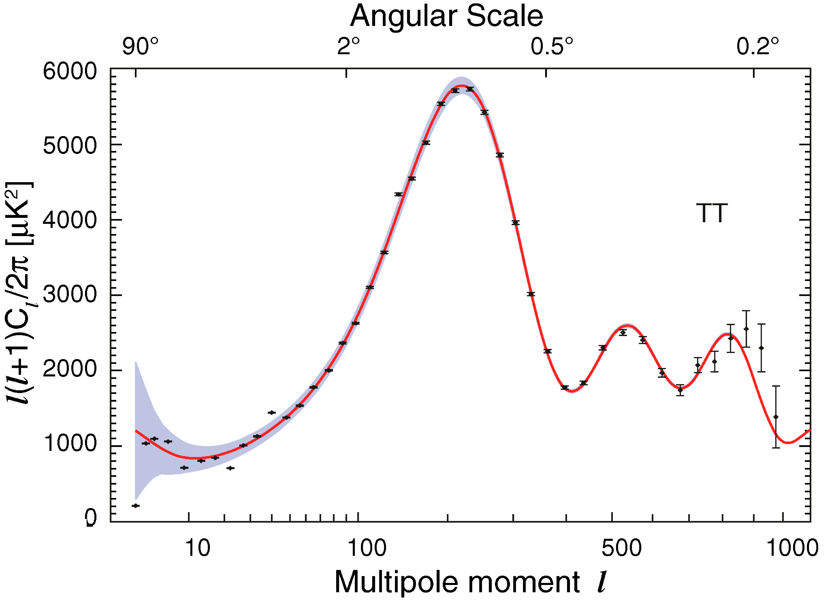
Visually, it is clear that the concordant model provides a reasonable fit to the data. Detailed analysis of the data indicates that $n_{{}_{\rm S}}\simeq 0.96$, when the tensor contribution is completely ignored. Whereas, it is found that $n_{{}_{\rm S}}\simeq 0.98$ when tensors are taken into account. The data also constrains the tensor-to-scalar ratio to $r<0.43$ at $95\%$ Confidence Level (CL) komatsu-2009a .

The slow roll approximation also enables specific inflationary models to be compared easily with the observations. In order to do so, firstly, note that, in the slow roll limit, upon using the corresponding background equations (35), the scalar and tensor spectral amplitudes (109) can be expressed in terms of the potential $V(\phi)$ and its derivative as follows bassett-2006 :

$${\cal P}_{{}_{\rm S}}(k) \simeq \left(\frac{1}{12\,\pi^{2}\,M_{{}_{\rm P}}^{6}}\right)\,\left(\frac{V^{3}}{V_{\phi}^{2}}\right)_{k=(a\,H)},$$ (114a)

$${\cal P}_{{}_{\rm T}}(k) \simeq \left(\frac{2}{3\,\pi^{2}}\right)\,\left(\frac{V}{M_{{}_{\rm P}}^{4}}\right)_{k=(a\,H)}.$$ (114b)

Secondly, during slow roll, the relations between the HSR and the PSR parameters can be obtained to be

$$\epsilon_{{}_{\rm H}}\simeq\epsilon_{{}_{\rm V}}\quad{\rm and}\quad\delta_{{}_{\rm H}}\simeq\left(\eta_{{}_{\rm V}}-\epsilon_{{}_{\rm V}}\right),$$ (115)

and, as a result, for instance, $\epsilon_{{}_{\rm V}}\simeq 1$ indicates the end of inflation. Let us now use these expressions to arrive at observational constraints on the parameters of a couple of inflationary models.

Observations indicate that the amplitude of the scalar perturbation associated with a mode that crossed the Hubble radius about $60$ $e$-folds before the end of inflation is about $\left(2\times 10^{-9}\right)$, a constraint that is referred to as the COBE normalization bunn-1996 . Given a potential, the expressions (112)–(115) allow us to construct the scalar amplitude and spectral index as well as the tensor-to-scalar ratio in terms of the inflaton. Let me now focus on the large field models (27) that I had discussed earlier. In these models, inflation ends (i.e. $\epsilon_{{}_{\rm V}}\simeq 1$), when $\phi_{\rm end}\simeq[(n/\sqrt{2})\,M_{{}_{\rm P}}]$. The value of the field at $N$ $e$-folds before the end inflation can be obtained using the solution (40a), and is given by $\phi_{{}_{N}}\simeq(\sqrt{[(4\,N+n)\,n/2]}\;M_{{}_{\rm P}})$. Using these expressions, it is straightforward to show that, for $V_{0}=(m^{2}/2)$ and $n=2$, the COBE normalization condition leads to the constraint that $m\simeq(10^{-5}\,M_{{}_{\rm P}}$). Similarly, for $V_{0}=(\lambda/4)$ and $n=4$, the condition leads to $\lambda\simeq 10^{-13}$.

The CMB observations also lead to useful constraints on the models in the $n_{{}_{\rm S}}$-$r$ plane. The various quantities that we have obtained above allow us to express the scalar spectral index and the tensor-to-scalar ratio in terms of the number of $e$-folds $N$ counted from the end inflation. For the large field models, the solution (40a) enables us to arrive at the following expressions in the slow roll limit bassett-2006

$$n_{{}_{\rm S}}\simeq 1-\left[\frac{2\,(n+2)}{4\,N+n}\right]\quad{\rm and}\quad r\simeq\left(\frac{16\,n}{4\,N+n}\right).$$ (116)

I have already shown that, for the case of power law inflation (19) described by the potential (21), $n_{{}_{\rm S}}$ and $r$ are constants given by Eqs. (97) and (98), respectively. These results for the power law case were exact. In the slow roll limit (i.e. when $q\gg 1$), they reduce to komatsu-2009a

$$n_{{}_{\rm S}}\simeq 1-\left(\frac{2}{q}\right)\quad{\rm and}\quad r=\left(\frac{16}{q}\right).$$ (117)

These relations indicate that these models will be described by straight lines in the $n_{{}_{\rm S}}$-$r$ plane. In Fig. 3, the joint constraints on the $n_{{}_{\rm S}}$-$r$ plane from the recent WMAP data (and a couple of other datasets) have been displayed komatsu-2009a .

Figure 3: Joint constraints on the $n_{{}_{\rm S}}$-$r$ plane from the WMAP $5$ year data, and a couple of other data sets. The contours indicate the $68\%$ and $95\%$ CLs derived from the data. The top panel clearly points to the fact that the data excludes the $n=4$ large field model at more than $95\%$ CL for $N<60$ (the solid line). In contrast, the $n=2$ model (the dashed line) performs better, and falls at the boundary of the $68\%$ region for $N=60$. (I should again stress that the number of $e$-folds have been counted backwards from the end of inflation.) The bottom panel indicates the behavior of power law inflation in the slow roll limit (i.e. when $q\ll 1$). It is evident that, while models with $q<60$ are outside of the $95\%$ region, models with $q\simeq 120$ lie close to the boundary of the $68\%$ region. (Note that $p$ in the bottom panel is what I have called as $q$. This figure is from Ref. komatsu-2009a , and I would refer the reader to this reference for any further details.)

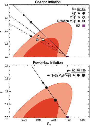
The behavior of a few inflationary models have been included in the figure as well. It is evident from the figure that, amongst the large field models, the $n=2$ case performs better than the $n=4$ case. Also, in the case of the power law inflation, it is found that $q<60$ is excluded at more than $95\%$ CL.

VII Status and prospects of inflation

I shall finally close by briefly commenting on the status and some prospects of the inflationary paradigm.

VII.1 Profusion of inflationary models

As a broad concept, inflation can certainly be considered as a success. However, a specific model of inflation that can be satisfactorily embedded in a high energy theory still eludes us. A plethora of inflationary models exist, quite a few of which are phenomenological in nature. Despite the enormous amount of effort, including attempts at considering models that are not described by the canonical action, it will be fair to say that we do not yet have a satisfactory model. The principal hurdle facing the idea of inflation is to construct a model that is well motivated from the high energy perspective, and also fits the observational data well.

VII.2 Features in the primordial spectrum

In this review, I had restricted myself to discussions on slow roll inflation, which leads to a featureless and nearly scale invariant primordial spectrum that seems to agree well with the recent observations of the CMB anisotropies. Though the agreement is rather good, there also exist a few points at the lower multipoles of the observed CMB angular power spectrum which lie outside the cosmic variance associated with the concordant model. Given these observations, a handful of model independent approaches have been constructed to recover the primordial power spectrum. At the smaller scales, all these approaches arrive at a spectrum that is nearly scale invariant. However, many of the approaches seem to unambiguously point to a sharp drop in power (along with a few distinct features) at the scales corresponding to the Hubble scale today. If future observations support the presence of such features in the primordial spectrum, then it poses an interesting challenge to build inflationary models that lead to the required spectrum. Conversely, the necessities of features will considerably restrict the class of allowed models of inflation. (For various efforts in this direction, see the references listed in Refs. pi ; tsr-pi .)

VII.3 Deviations from Gaussianity

I had earlier mentioned that the scalar perturbations generated during inflation are Gaussian in nature. I had also clarified that this was primarily due to the fact that we had confined ourselves to linear perturbation theory. Deviations from Gaussianity can arise when takes into account the perturbations at the higher orders bartolo-2004a ; bartolo-2004b . However, the extent of the non-Gaussianity depends on a variety of reasons (for a recent discussion on the issue and further references, see Ref. komatsu-2009b ). Interestingly, recent re-analysis of the WMAP $5$-year data seem to indicate sufficiently large non-Gaussianities (see, for instance, Ref. smith-2009 ). If future observations confirm such a large level of non-Gaussianity, then, it can result in a substantial tightening in the constraints on the inflationary models. For example, canonical scalar field models that lead to a nearly scale invariant primordial spectrum contain only a small amount of non-Gaussianity and, hence, may cease to be viable maldacena-2003 . However, it is known that primordial spectra with features can lead to reasonably large non-Gaussianities chen-2007a ; chen-2007b . Therefore, if non-Gaussianity indeed turns out to be large, then, either one may have to reconcile with the fact that the primordial spectrum contains features, or one possibly have to seriously consider models described by non-canonical actions, some of which are known to result in large Gaussianities (see, for instance, Refs. langlois-2008a ; langlois-2008b ).

Hopefully, one or both of these aspects will help us arrive at a satisfactory model of inflation.