Inflationary Cosmological Perturbations of Quantum-Mechanical Origin

This review article aims at presenting the theory of inflation. We first describe the background spacetime behavior during the slow-roll phase and analyze how inflation ends and the Universe reheats. Then, we present the theory of cosmological perturbations with special emphasis on their behavior during inflation. In particular, we discuss the quantum-mechanical nature of the fluctuations and show how the uncertainty principle fixes the amplitude of the perturbations. In a next step, we calculate the inflationary power spectra in the slow-roll approximation and compare these theoretical predictions to the recent high accuracy measurements of the Cosmic Microwave Background radiation (CMBR) anisotropy. We show how these data already constrain the underlying inflationary high energy physics. Finally, we conclude with some speculations about the trans-Planckian problem, arguing that this issue could allow us to open a window on physical phenomena which have never been probed so far.

1 Introduction

Inflation is the most promising theory of the early Universe. It was invented by A. Guth guth at the beginning of the $80$’s in order to solve the puzzles of the hot Big Bang theory. A very interesting aspect of the inflationary theory is that it allows us to build a bridge between cosmology and high energy physics. This is particularly valuable in view of the fact that it is difficult to probe physics beyond the standard model of particular physics.

However, the details of the underlying particle physics model are encoded into the fine structure of the cosmological observables. This is why, after the invention of the inflationary scenario and during quite a long time, it was in fact only possible to check the consistency of the inflationary predictions. The situation has now changed drastically with the recent releases of very high accuracy cosmological data. One can now take advantage of the full predictive power of inflation with the hope to learn about physics in a regime which has never been reached before.

The goal of this review article is to give a general presentation of the inflationary scenario. In particular, we will emphasize how the origin of the inhomogeneities present in our Universe is explained in the framework of inflation. We will see that it is based on an elegant interplay between general relativity and quantum theory. Then, we will present the corresponding predictions made by inflation and will study how the currently available data can already put some constraints on the underlying particle physics models.

This article is organized as follows. In the next section, we describe the evolution of the inflationary background, the slow-roll phase and the reheating. Then, we present the theory of cosmological perturbations of quantum-mechanical origin and compare its predictions to the available data. Finally, we conclude this article with some speculations concerning the trans-Planckian problem of inflation, demonstrating that future astrophysical observations will maybe open a new window on high energy physics.

2 The Inflationary Universe

2.1 Basic Equations

The cosmological principle implies that the Universe is, on large scales, homogeneous and isotropic. As a consequence, the metric tensor which describes the geometry of the Universe is of the Friedman-Lemaître-Robertson-Walker (FLRW) form, namely

$${\rm d}s^{2}=-c^{2}{\rm d}t^{2}+a^{2}(t)\gamma_{ij}^{(3)}{\rm d}x^{i}{\rm d}x^{j}=a^{2}(\eta)\left[-{\rm d}\eta^{2}+\gamma_{ij}^{(3)}{\rm d}x^{i}{\rm d}x^{j}\right]\,,$$ (1)

where $\gamma_{ij}^{(3)}$ is the metric of the three-dimensional spacelike sections. The three-dimensional sections have a constant scalar curvature. The variable $t$ is the cosmic time while $\eta$ is the conformal time. They are linked by the relation $c{\rm d}t=a{\rm d}\eta$. In this article, we will work with dimensionless coordinates $x^{i}$ and, as a consequence, the scale factor $a(\eta)$ will have the dimension of a length.

The matter is assumed to be a collection of $N$ perfect fluids and therefore its stress-energy tensor is given by the following expression

$$T_{\mu\nu}=\sum_{i=1}^{N}T_{\mu\nu}^{(i)}=(\rho_{{}_{\rm T}}+p_{{}_{\rm T}})u_{\mu}u_{\nu}+p_{{}_{\rm T}}g_{\mu\nu}\,,$$ (2)

where $\rho_{{}_{\rm T}}$ is the (total) energy density and $p_{{}_{\rm T}}$ the (total) pressure. These two quantities are linked by the equation of state, $p_{{}_{\rm T}}=\omega\left(\rho_{{}_{\rm T}}\right)$ [in general, there is an equation of state per fluid considered, i.e. $p_{i}=\omega_{i}(\rho_{i})$]. The vector $u_{\mu}$ is the four velocity and satisfy the relation $u_{\mu}u^{\mu}=-1$. This means that one has $u^{\mu}=(1/a,0)$ and $u_{\mu}=(-a,0)$. The fact that the stress-energy tensor is conserved, $\nabla^{\alpha}T_{\alpha\mu}=0$, amounts to

$$\rho_{{}_{\rm T}}^{\prime}+3\frac{a^{\prime}}{a}(\rho_{{}_{\rm T}}+p_{{}_{\rm T}})=0\,.$$ (3)

This expression is obtained from the $\mu=0$ component. The component $\mu=i$ does not lead to an interesting equation for the background. If one assumes that each fluid is separately conserved then the above equation is valid for each species.

We will assume that gravity is correctly described by the theory of General Relativity even in the very early Universe. This means that the equations which link the geometrical part to the matter part are nothing but the Einstein equations

$$R_{\mu\nu}-\frac{1}{2}Rg_{\mu\nu}=\kappa T_{\mu\nu}\,,$$ (4)

where $\kappa\equiv 8\pi G/c^{4}=8\pi/m_{{}_{\rm Pl}}^{2}$. These equations, in the case of a FLRW Universe, are differential equations determining the time evolution of the scale factor and read

$$\frac{3}{a^{2}}\biggl{[}\biggl{(}\frac{a^{\prime}}{a}\biggr{)}^{2}+k\biggr{]}=\kappa\sum_{i=1}^{N}\rho_{i},\quad-\frac{1}{a^{2}}\biggr{[}2\frac{a^{\prime\prime}}{a}-\biggl{(}\frac{a^{\prime}}{a}\biggr{)}^{2}+k\biggr{]}=\kappa\sum_{i=1}^{N}p_{i}\,,$$ (5)

where a prime denotes a derivative with respect to conformal time. In the following, we will use the definition ${\cal H}\equiv a^{\prime}/a$. The parameter $k=0,\pm 1$ represents the curvature of the spacelike sections. If, in addition, the equation of state of the perfect fluids are provided, then we have a closed system of differential equations and, therefore, the evolution of the corresponding model of the Universe is completely specified.

2.2 The Inflationary Hypothesis

By definition, inflation is a phase of accelerated expansion, i.e. the scale factor satisfies inflation

$$\frac{{\rm d}^{2}a}{{\rm d}t^{2}}>0\,.$$ (6)

It is interesting to postulate that such a phase took place in the very early Universe because, in this case, one can explain many different seemingly paradoxical facts like, for instance, the horizon problem or the flatness problem. Because of the latter, from now on, we will put $k=0$ in the Einstein equations. More precisely, one can show the inflationary scenario is satisfactory if the number of e-folds, i.e. the logarithm of the scale factor at the end of inflation to the scale factor at the beginning of inflation is greater than $60$ inflation ,

$$N_{{}_{\rm T}}>60\,.$$ (7)

More detailed arguments about the advantages of inflation can be found in Ref. procbrazil but, at this point, it is important to notice the following three facts. Firstly, inflation is convincing because, by means of a single concept or hypothesis, one can solve many different problems. In this sense, inflation is an economical assumption. Secondly, as we will show below, inflation is falsifiable since it makes definite predictions that we will describe. Therefore, there is the hope either to confirm or to exclude this hypothesis and, in any case, there is the certainty to learn something about the early Universe. Thirdly, inflation is defined by the condition (6) but this does not prejudge the physical nature of the matter responsible for the acceleration of the Universe. The only thing one can say is obtained by expressing the acceleration of the scale factor in cosmic time. Using the Einstein equations, one gets

$$\frac{\ddot{a}}{a}=-\frac{\kappa}{6}(\rho+3p)\,,$$ (8)

where a dot denotes a derivative with respect to the cosmic time. Therefore, the fluid responsible for inflation must be such that

$$p<-\frac{\rho}{3}\,,$$ (9)

i.e. must have a negative pressure. As a consequence, this fluid cannot be a standard fluid, like a gas for instance, but must be somehow “exotic”. However, this does not come as a surprise since inflation is supposed to take place at very high energies. At those energies, the natural description of matter is (quantum) field theory. As we are now going to demonstrate, it is quite interesting to remark that the most simple example of a field theory can do the job very well and “produce” the negative pressure which is necessary to inflation. We now discuss this point in more details.

2.3 Implementing the Inflationary Hypothesis

The most simple implementation of the inflationary scenario is to assume that matter is described by a scalar field $\varphi(\eta)$ guth ; inflation . This case is nothing but a particular example of a perfect fluid. The corresponding action reads

$$S=-\int{\rm d}^{4}x\sqrt{-g}\biggl{[}\frac{1}{2}g^{\mu\nu}\partial_{\mu}\varphi\partial_{\nu}\varphi+V(\varphi)\biggr{]}\,.$$ (10)

Then, the stress-energy tensor, which is defined by

$$T_{\mu\nu}=-\frac{2}{\sqrt{-g}}\frac{\delta S}{\delta g^{\mu\nu}}\,,$$ (11)

can be written as

$$T_{\mu\nu}=\partial_{\mu}\varphi\partial_{\nu}\varphi-g_{\mu\nu}\biggl{[}\frac{1}{2}g^{\alpha\beta}\partial_{\alpha}\varphi\partial_{\beta}\varphi+V(\varphi)\biggr{]}\,.$$ (12)

From this expression, it is clear that the scalar field is indeed a perfect fluid. The energy density and the pressure are defined by $T^{0}{}_{0}=-\rho$, $T^{i}{}_{j}=p\delta^{i}{}_{j}$ and we obtain

$$\rho=\frac{1}{2}\frac{(\varphi^{\prime})^{2}}{a^{2}}+V(\varphi),\quad p=\frac{1}{2}\frac{(\varphi^{\prime})^{2}}{a^{2}}-V(\varphi)\,.$$ (13)

The conservation equation can be obtained either by re-deriving it from the very beginning or just by inserting the previous expressions of the energy density and pressure into Eq. (3). Assuming $\varphi^{\prime}\neq 0$, this reproduces the Klein-Gordon equation written in a FLRW background, namely

$$\varphi^{\prime\prime}+2\frac{a^{\prime}}{a}\varphi^{\prime}+a^{2}\frac{{\rm d}V(\varphi)}{{\rm d}\varphi}=0\,.$$ (14)

The other equation of conservation expresses the fact that the scalar field is homogeneous and, therefore, does not bring any new information. Finally, a comment is in order about the equation of state. In general, there is no simple link between $\rho$ and $p$ except when the kinetic energy dominates the potential energy, where $\omega\equiv p/\rho\simeq 1$, i.e. the case of stiff matter or, on the contrary, when the potential energy dominates the kinetic energy for which one obtains $\omega\simeq-1$. This last case is of course very interesting since this leads to an inflationary solution. We have thus identified the condition under which inflation can occur: the potential energy must dominate the kinetic energy, i.e.

$$V(\varphi)\gg\frac{1}{2}\frac{(\varphi^{\prime})^{2}}{a^{2}}\,.$$ (15)

We now turn to a systematic study of this regime.

2.4 Slow-roll Inflation

Since the kinetic energy to potential energy ratio and the scalar field acceleration to the scalar field velocity ratio are small, this suggests to view these quantities as parameters in which a systematic expansion is performed. The slow roll regime is controlled by the three (at leading order) slow-roll parameters defined by:

$$\epsilon \equiv 3\frac{\dot{\varphi}^{2}}{2}\left(\frac{\dot{\varphi}^{2}}{2}+V\right)^{-1}=-\frac{\dot{H}}{H^{2}}=1-\frac{{\cal H}^{\prime}}{{\cal H}^{2}}\,,$$ (16)

$$\delta \equiv -\frac{\ddot{\varphi}}{H\dot{\varphi}}=-\frac{\dot{\epsilon}}{2H\epsilon}+\epsilon\ ,\quad\xi\equiv\frac{\dot{\epsilon}-\dot{\delta}}{H}\ .$$ (17)

The slow-roll conditions are satisfied if $\epsilon$ and $\delta$ are much smaller than one and if $\xi={\cal O}(\epsilon^{2},\delta^{2},\epsilon\delta)$. It is also convenient to re-express the slow-roll parameters in terms of the inflaton potential. Using the equations of motion in the slow-roll approximation, one can show that

$$\epsilon\simeq\frac{m_{{}_{\rm Pl}}^{2}}{16\pi}\biggl{(}\frac{V^{\prime}}{V}\biggr{)}^{2},\quad\delta\simeq-\frac{m_{{}_{\rm Pl}}^{2}}{16\pi}\biggl{(}\frac{V^{\prime}}{V}\biggr{)}^{2}+\frac{m_{{}_{\rm Pl}}^{2}}{8\pi}\frac{V^{\prime\prime}}{V}\,,$$ (18)

where, here, a prime denotes a derivative with respect to the scalar field.

The equations of motion, that is to say the Friedman equation and the Klein-Gordon equation can be re-written exactly as

$$H^{2}=\frac{\kappa V}{3-\epsilon}\,,\quad\frac{{\rm d}\varphi}{{\rm d}t}=-\frac{1}{(3-\delta)H}\frac{{\rm d}V}{{\rm d}\varphi}\,,$$ (19)

from which one deduces that, if the slow-roll conditions are satisfied

$$H^{2}\simeq\frac{\kappa}{3}V(\varphi)+{\cal O}\left(\epsilon\right)\,,\quad\frac{{\rm d}\varphi}{{\rm d}t}\simeq-\frac{1}{3H}\frac{{\rm d}V}{{\rm d}\varphi}+{\cal O}\left(\delta\right)\,.$$ (20)

These equations are of course easier to analyze and solve than the original ones.

Let us now analyze a concrete example. We choose the following class of potentials

$$V(\varphi)=\frac{3\lambda_{n}}{8\pi}m_{{}_{\rm Pl}}^{4}\left(\frac{\varphi}{m_{{}_{\rm Pl}}}\right)^{n}\,,$$ (21)

where $n$ is a free parameter and $\lambda_{n}$ the coupling constant. The factors that show up into the definition of the potential have been chosen for future convenience. Let us first try to see under which conditions the slow-roll approximation is valid. We adopt the criterion $\epsilon<1$ (it is in fact $\epsilon\ll 1$ and , strictly speaking, $\epsilon<1$ only corresponds to the condition necessary in order to have an accelerated expansion). This amounts to

$$\varphi>\varphi_{\rm end}=\frac{n}{4\sqrt{\pi}}m_{{}_{\rm Pl}}\,.$$ (22)

Of course, this constraint applies in particular to the initial value of the field. We already conclude, that for this class of models, the values of the field must be at least a few Planck mass. Let us be more precise and evaluate the total number of e-folds during slow-roll inflation. It is given by the formula

$$N_{{}_{\rm T}}=\ln\biggl{(}\frac{a_{\rm end}}{a_{\rm ini}}\biggr{)}\simeq-\kappa\int_{\varphi_{\rm ini}}^{\varphi_{\rm end}}{\rm d}\varphi V(\varphi)\biggl{(}\frac{{\rm d}V}{{\rm d}\varphi}\biggr{)}^{-1}\,,$$ (23)

from which one gets

$$N_{{}_{\rm T}}=\frac{4\pi}{n}\left(\frac{\varphi_{\rm ini}}{m_{{}_{\rm Pl}}}\right)^{2}-\frac{n}{4}\,.$$ (24)

Let $N_{\rm min}$ the minimum number of e-folds required in order to solve the problems of the hot big-bang model (we have seen before that $N_{\rm min}\simeq 60$) then one has

$$\varphi_{\rm ini}>m_{{}_{\rm Pl}}\sqrt{\frac{n}{4\pi}\left(N_{\rm min}+\frac{n}{4}\right)}\,.$$ (25)

For $n=2$, this gives $\varphi_{\rm ini}\simeq 3.1m_{{}_{\rm Pl}}$ and for $n=4$, one obtains $\varphi_{\rm ini}\simeq 4.4m_{{}_{\rm Pl}}$. However, it is often argued that “natural” initial conditions (see the last article in Refs. inflation ) are such that $V(\varphi_{\rm ini})=m_{{}_{\rm Pl}}^{4}$ which amounts to

$$\varphi_{\rm ini}=m_{{}_{\rm Pl}}\left(\frac{8\pi}{3}\right)^{1/n}\lambda_{n}^{-1/n}\gg m_{{}_{\rm Pl}}\,,$$ (26)

because, as we will discuss later one, the COsmic Background Explorer (COBE) normalization implies that the coupling constant is small. In this case, the number of e-folds is a large number, much larger that the minimum required. Of course, the fact that the value of the scalar field must be larger or of the order of the Planck mass has led to many discussions about the model building problem. In this review, we do not address this question. Details about this issue can be found in Refs. LR ; Linde .

Let us now solve the equations of motions in the slow-roll approximation. For the scalar field straightforward calculations lead to ($n\neq 4$)

$$\varphi(t)=\varphi_{\rm ini}\left[1-\frac{n(4-n)}{2}\frac{\sqrt{\lambda_{n}}}{8\pi}\left(\frac{m_{{}_{\rm Pl}}}{\varphi_{\rm ini}}\right)^{(4-n)/2}m_{{}_{\rm Pl}}(t-t_{\rm ini})\right]^{2/(4-n)}\,.$$ (27)

The last expression can also be expressed in terms of $t_{\rm end}$, the time at which slow-roll inflation stops. One obtains

$$\varphi(t)=\varphi_{\rm ini}\left\{1-\frac{t-t_{\rm ini}}{t_{\rm end}-t_{\rm ini}}\left[1-\left(\frac{\varphi_{\rm end}}{\varphi_{\rm ini}}\right)^{(4-n)/2}\right]\right\}^{2/(4-n)}\,.$$ (28)

The advantage of the above equation is to show that for $t<t_{\rm end}$ the argument between braces always remains positive and hence the whole expression well-defined. A negative argument would simply signal the break-down of the slow-roll approximation and, in this case, the above formula cannot be used.

Let us now turn to the scale factor. Integrating the first of Eqs. (20) leads to

$$a(t)=a_{\rm ini}\exp\left\{-\frac{4\pi}{nm_{{}_{\rm Pl}}^{2}}\left[\varphi_{0}^{2}(t)-\varphi_{\rm ini}^{2}\right]\right\}\,.$$ (29)

From this expression, one can also calculate the evolution of the scalar field in terms of the number of e-folds $N$ which is the natural time variable during inflation. One gets

$$\varphi(N)=m_{{}_{\rm Pl}}\sqrt{\left(\frac{\varphi_{\rm ini}}{m_{{}_{\rm Pl}}}\right)^{2}-\frac{n}{4\pi}N}\,,$$ (30)

from which one obtains the formula giving the evolution of the Hubble parameter during inflation

$$H(N)=m_{{}_{\rm Pl}}\sqrt{\lambda_{n}}\left[\left(\frac{\varphi_{\rm ini}}{m_{{}_{\rm Pl}}}\right)^{2}-\frac{n}{4\pi}N\right]^{n/4}\,.$$ (31)

This equation is valid until $N=N_{{}_{\rm T}}$ and, in this regime, the above formula is always well-defined. Indeed, Eq. (31) becomes meaningless at $N_{\rm max}=4\pi(\varphi_{\rm ini}/m_{{}_{\rm Pl}})^{2}/n$ but $N_{\rm max}>N_{{}_{\rm T}}$. The above equation has interesting consequences for our understanding of inflation. It shows that the Hubble parameter can evolve and change significantly during the slow-roll phase. Later on, we will see that a quantity which plays an important role is the value of the Hubble parameter when the scales of astrophysical interest today crossed out the horizon during inflation. This happens $60$ e-folds before the end of inflation. This scale is constrained by the observations on the Cosmic Microwave Background Radiation (CMBR) anisotropies to be $H/m_{{}_{\rm Pl}}<10^{-5}$. However, this does not mean that the Hubble parameter has not been larger before, especially if the total number of total e-folds is large, as it is the case for the initial conditions discussed in Eq. (26). For instance, if we have a massive potential, $n=2$, and $\varphi_{\rm ini}=100\,m_{{}_{\rm Pl}}$ then inflation starts with an initial Hubble parameter of $H_{\rm ini}\simeq 10^{-3}m_{{}_{\rm Pl}}$ but ends at $H_{\rm end}=m_{{}_{\rm Pl}}\sqrt{\lambda_{n}}\left[n/\left(4\sqrt{\pi}\right)\right]^{n/2}\simeq 0.28\times 10^{-5}m_{{}_{\rm Pl}}$ after $N\simeq 62000$ e-folds, where we have used $\lambda_{2}\simeq 10^{-10}$ (corresponding to a mass $m\simeq 10^{-5}m_{{}_{\rm Pl}}$). Therefore, in summary, it will be important to keep in mind that the observations give indications about the scale of inflation when the relevant scales crossed out the horizon during inflation but cannot, a priori, put constrains on the Hubble parameter in the earliest phases of evolution.

Figure 1: Evolution of the various scales discussed in the text during inflation and the subsequent radiation and matter dominated epochs. In particular, it is apparent that the CMBR measurements only probe the inflationary model when the modes of astrophysical interest today crossed out the horizon during inflation. The small window shows a typical inflationary potential, see Eq. (21).

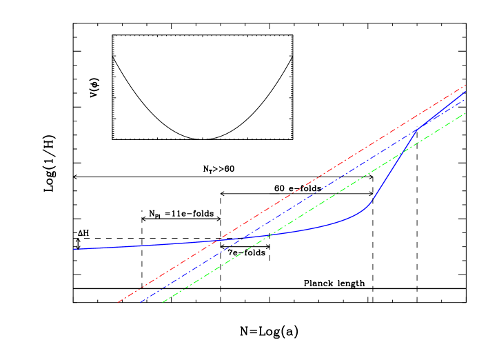
This situation is summarized in Fig. 1.

When the field reaches the value $\varphi_{\rm end}$, slow-roll inflation stops and the system enters a new regime that we now briefly describe.

2.5 Reheating

When the scalar field reaches the point where the slow-roll parameter $\epsilon\simeq 1$, for which $\varphi=\varphi_{\rm end}$, inflation stops and the field starts oscillating around its minimum turner ; preheating . In this regime, the system is governed by two time scales: the Hubble time $H^{-1}$ and the period of the oscillations around the minimum $(V^{\prime\prime})^{-1}$ (here, a prime means derivative with respect to the field). The important point is that these two scales are very different. The frequency of the oscillations is much larger than the Hubble rate, $\omega_{\rm osci}\simeq V^{\prime\prime}\gg H$. The scalar field obeys the Klein-Gordon equation which can be put under the following form

$$\frac{{\rm d}\rho}{{\rm d}t}=-3H\dot{\varphi}^{2}=-6H(\rho-V)\,,$$ (32)

where the relation $\dot{\varphi}^{2}=2(\rho-V)$ has been used. This equation can be time averaged and one gets

$$\biggl{\langle}\frac{{\rm d}\rho}{{\rm d}t}\biggr{\rangle}=-\bigl{\langle}6H(\rho-V)\bigr{\rangle}\simeq-6H\bigl{\langle}\rho-V\bigr{\rangle}\,,$$ (33)

where we have used the fact that the Hubble rate does not change during one period of the oscillations. The right hand side of the equation above can be evaluated as

$$\bigl{\langle}\rho-V\bigr{\rangle}\equiv\frac{1}{T}\int_{0}^{T}(\rho-V){\rm d}t=\left[\int_{-\varphi_{\rm m}}^{\varphi_{\rm m}}\sqrt{\rho-V(\varphi)}{\rm d}\varphi\right]\left[\int_{-\varphi_{\rm m}}^{\varphi_{\rm m}}\frac{{\rm d}\varphi}{\sqrt{\rho-V(\varphi)}}\right]^{-1}\,,$$ (34)

where $\varphi_{\rm m}$ is the value of the scalar field at the maximum of its oscillations. In order to obtain the previous relation, one has also utilized that ${\rm d}t={\rm d}\varphi/\sqrt{2(\rho-V)}$. Then, one uses that over one period, $\rho\simeq V(\varphi_{\rm m})\equiv V_{\rm m}$ is a constant and one obtains

$$\bigl{\langle}\rho-V\bigr{\rangle}\simeq\gamma\rho\,,$$ (35)

where the number $\gamma$ is defined by

$$\gamma\equiv\left[\int_{-\varphi_{\rm m}}^{\varphi_{\rm m}}\sqrt{1-\frac{V(\varphi)}{V_{\rm m}}}{\rm d}\varphi\right]\left\{\int_{-\varphi_{\rm m}}^{\varphi_{\rm m}}\left[1-\frac{V(\varphi)}{V_{\rm m}}\right]^{-1/2}{\rm d}\varphi\right\}^{-1}=\frac{n}{n+2}\,,$$ (36)

the last result being valid for potentials of the form $V(\varphi)\propto\varphi^{n}$. Let us now turn to the left hand side of Eq. (33). The term $\langle{\rm d}\rho/{\rm d}t\rangle$ can be written as $\Delta\rho/T$. It can be expressed as a finite difference expression and one can rewrite it as $\dot{\rho}$. This is valid for time intervals much larger than the period of the oscillations. Therefore, the equation governing the evolution of the energy density of the field (33) can be rewritten as

$$\dot{\rho}=-\frac{6n}{n+2}H\rho\Rightarrow\rho\propto a^{-6n/(n+2)}\,.$$ (37)

Then, the scale factor is given by $a(t)\propto t^{(n+2)/(3n)}$. For the massive case, $n=2$, the energy density evolves as in a matter-dominated epoch. This can be easily understood since, in this case, the Klein-Gordon equation is exactly the equation of an harmonic oscillator. In this situation, it is known that $\langle\dot{\varphi}^{2}/2\rangle=\langle V(\varphi)\rangle$ which implies that the pressure vanishes.

So far, we have not taken into account the effect of particles creation. Phenomenologically, it can be described by adding a term $\Gamma\dot{\varphi}$ in the Klein-Gordon equation which now reads

$$\ddot{\varphi}+3H\dot{\varphi}+\Gamma\dot{\varphi}+\frac{{\rm d}V(\varphi)}{{\rm d}\varphi}=0\quad\Rightarrow\frac{{\rm d}\rho}{{\rm d}t}=-\frac{2n}{n+2}(3H+\Gamma)\rho.$$ (38)

If we assume that the particles produced are very light in comparison with the mass of the inflaton, these particles will be very relativistic. This means that the equation of conservation of radiation should also be modified according to

$$\frac{{\rm d}\rho_{\rm r}}{{\rm d}t}=-4H\rho_{\rm r}+\Gamma\rho\,,$$ (39)

so that the total energy is still conserved. Eq. (38) can be easily integrated and the solution reads

$$\rho(t)=\rho_{\rm osci}\biggl{(}\frac{a}{a_{\rm osci}}\biggr{)}^{-6n/(n+2)}\exp\biggl{[}-\frac{2n}{n+2}\Gamma(t-t_{\rm osci})\biggr{]}\,$$ (40)

where $t=t_{\rm osci}$ is the time at which the oscillations start (i.e. the time at which the slow-roll period ends) and $\rho_{\rm osci}$ is the value of the scalar field energy density at that time. The effect of the term $\Gamma\dot{\varphi}$ is to multiply the result (37) by a decreasing exponential factor. Equipped with this solution, we can solve Eq. (39) and determine the evolution of $\rho_{\rm r}$. If the scalar field energy density dominates the radiation, as it is the case at the beginning of the reheating period, the solution reads (using the fact that the scale factor is known in this regime, see above)

$$\rho_{\rm r}(t) = \Gamma t_{\rm osci}\rho_{\rm osci}\biggl{(}\frac{a}{a_{\rm osci}}\biggr{)}^{-4}\biggl{(}\frac{n+2}{2n\Gamma t_{\rm osci}}\biggr{)}^{(n+8)/(3n)}\exp\biggl{(}\frac{2n}{n+2}\Gamma t_{\rm osci}\biggr{)}$$ (41)

$$\times\biggl{[}\gamma\biggl{(}\frac{n+8}{3n},\frac{2n}{n+2}\Gamma t\biggr{)}-\gamma\biggl{(}\frac{n+8}{3n},\frac{2n}{n+2}\Gamma t_{\rm osci}\biggr{)}\biggr{]}\,,$$

where the function $\gamma(\alpha,x)$ is the incomplete gamma function defined by $\gamma(\alpha,x)\equiv\int_{0}^{x}{\rm e}^{-t}t^{\alpha-1}{\rm d}t$. In the above formula, we have assumed that, at the end of the slow-roll epoch $t=t_{\rm osci}$, $\rho_{\rm r}\simeq 0$. For small values of the argument $x$, the incomplete gamma function reduces to $\simeq x^{\alpha}/\alpha$. We define $t_{{}_{\rm RH}}\equiv\Gamma^{-1}$ and then we have $x=2n\Gamma t/(n+2)=2n/(n+2)(t/t_{{}_{\rm RH}})$ and for times $t>t_{\rm osci}\ll\Gamma^{-1}$, the argument of the incomplete gamma function is small. In this limit, one obtains

$$\rho_{\rm r}(t)\simeq\Gamma\rho_{\rm osci}t_{\rm osci}^{2}\frac{3n}{(n+8)t}\biggl{[}1-\biggl{(}\frac{t}{t_{\rm osci}}\biggr{)}^{-(n+8)/(3n)}\biggr{]}\,.$$ (42)

We see that $\rho_{\rm r}$ starts to increase, reaches a maximum and then decreases. When $t$ approaches $t_{{}_{\rm RH}}$, the previous approximation breaks down since the argument of the incomplete gamma function is no longer small. However, for order of magnitude estimates, we can try to push this approximation. At $t\simeq t_{{}_{\rm RH}}$, we have $\rho_{\rm r}\simeq\Gamma\rho_{\rm osci}t_{\rm osci}^{2}3n/[(n+8)t_{{}_{\rm RH}}]$ since the second term in the square bracket in Eq. (42) is negligible. After thermalization, the energy density of radiation takes the form $\rho_{\rm r}=g_{*}\pi^{2}T^{4}/30$. Using the fact that $\rho_{\rm osci}\simeq H_{\rm inf}^{2}m_{{}_{\rm Pl}}^{2}$ (nothing but the Friedman equation) and that $t_{\rm osci}\simeq H_{\rm inf}^{-1}$, one can deduce the reheating temperature

$$T_{{}_{\rm RH}}\simeq\frac{30^{1/4}}{\sqrt{\pi}}g_{*}^{-1/4}\biggl{(}\frac{3n}{n+8}\biggr{)}^{1/4}(\Gamma m_{{}_{\rm Pl}})^{1/2}\,.$$ (43)

Then, from this temperature, the universe evolves in a standard radiation dominated era. The remarkable feature of the previous equation is that it does not depend on the scale of inflation $H_{{}_{\rm inf}}$ but only on the decay rate $\Gamma$ of the inflaton. This means that whatever the scale of inflation is, the radiation dominated era always starts at the same energy (at fixed decay rate) and that the duration of the period of coherent oscillations can change quite a lot. The number of e-foldings during this epoch can be evaluated as [since during this epoch, the scale factor scales as $\propto t^{(n+2)/(3n)}$]

$$N\simeq\frac{n+2}{3n}\ln\biggl{(}\frac{H_{\rm inf}}{\Gamma}\biggr{)}\,.$$ (44)

The previous considerations are valid if the life time of the inflaton is bigger than the age of the universe at the end of inflation. Otherwise, there is no period of coherent oscillations. In this case, the vacuum energy $H_{\rm inf}^{2}m_{{}_{\rm Pl}}^{2}$ is directly converted into radiation and the reheating temperature is

$$T_{{}_{\rm RH}}\simeq\frac{30^{1/4}}{\sqrt{\pi}}g_{*}^{-1/4}(H_{\rm inf}m_{{}_{\rm Pl}})^{1/2}\,.$$ (45)

Finally, let us recall that the calculations above assume that the physical quantities are time averaged and therefore that the time scales considered are larger than the period of the oscillations.

Figure 2: Evolution of the scalar field during slow-roll inflation and the reheating phase (where the field oscillates) obtained by numerical integration of the equations of motion. The potential is of the type of Eq. (21) with $n=2$ and $\lambda_{2}=(8\pi/6)\times 10^{-10}$. The initial conditions are such that $\varphi_{\rm ini}\simeq 3m_{{}_{\rm Pl}}$ leading to $N_{{}_{\rm T}}\simeq 60$ as confirmed by the plot.

In Fig. 2, where the evolution of the field versus the number of e-folds is displayed, we have integrated the equations of motion numerically. This plot confirms our analytical estimates: inflation consists of a phase of slow-roll followed by a phase of oscillations. This concludes our study of the inflationary background.

3 Cosmological Perturbations

3.1 General Framework

It is an observational fact that the universe is not isotropic and homogeneous. Therefore, if one wants to have an accurate description, it is clearly mandatory to go beyond the FLRW model. On the other hand, it is also an experimental fact that, in the early Universe, the deviations from the isotropy and from the homogeneity were small (e.g. from the COBE measurement, $\delta T/T\simeq 10^{-5}$). This suggests a perturbative treatment. Therefore, the following metric tensor MFB gives a refined description of our Universe

$$\gamma_{\mu\nu}(\eta,\vec{x})=[g_{\mu\nu}(\eta)+\epsilon h_{\mu\nu}(\eta,\vec{x})+\epsilon^{2}\ell_{\mu\nu}(\eta,\vec{x})+\cdots]{\rm d}x^{\mu}{\rm d}x^{\nu}\,,$$ (46)

where $g_{\mu\nu}(\eta)$ is the standard FLRW metric introduced previously and represents the “background” (the parameter $\epsilon$ in the above equation should not be confused with the first slow-roll parameter; they have nothing to do with each other). The perturbed metric depends on $\vec{x}$ and this is the signature of the fact that we now go beyond the cosmological principle. In order to be consistent, the same expansion must be performed for the quantities describing matter. For example, if there is a background scalar field $\varphi(\eta)$, a refined description of the scalar field can be expressed as

$$\varphi(\eta,\vec{x})=\varphi(\eta)+\epsilon\delta\varphi(\eta,\vec{x})+\epsilon^{2}\delta^{(2)}\varphi(\eta,\vec{x})+\cdots\,.$$ (47)

The main goal of the theory of cosmological perturbations is to determine the evolution of the perturbed quantities $h_{\mu\nu}$ and $\delta\varphi$ and, then, to use them in order to calculate observable quantities. To find the behavior of the perturbed quantities, one needs some equations of motion. Naturally, these equations are taken to be the perturbed Einstein equations written order by order (we assume that gravity is described by General Relativity). Therefore, we expand the Einstein tensor and the stress-energy tensor according to

$$G_{\mu\nu}=G_{\mu\nu}^{(0)}+\epsilon G_{\mu\nu}^{(1)}+\epsilon^{2}G_{\mu\nu}^{(2)}+\cdots,\quad T_{\mu\nu}=T_{\mu\nu}^{(0)}+\epsilon T_{\mu\nu}^{(1)}+\epsilon^{2}T_{\mu\nu}^{(2)}+\cdots\,,$$ (48)

and then identify the terms of same order to obtain

$$G_{\mu\nu}^{(0)}=\kappa T_{\mu\nu}^{(0)},\quad G_{\mu\nu}^{(1)}=\kappa T_{\mu\nu}^{(1)},\quad G_{\mu\nu}^{(2)}=\kappa T_{\mu\nu}^{(2)},\cdots\,.$$ (49)

In the present context, we will restrict ourselves to the linear order in the parameter $\epsilon$.

Let us now try to describe the perturbed metric tensor in more details. For any symmetric two-rank tensor, there is a theorem stewart which states that $h_{\mu\nu}(\eta,\vec{x})$ can be decomposed as $h_{\mu\nu}(\eta,\vec{x})=h_{\mu\nu}^{\rm(S)}+h_{\mu\nu}^{\rm(V)}+h_{\mu\nu}^{\rm(T)}$, where $h_{\mu\nu}^{\rm(S)}$ is constructed only from scalar functions, $h_{\mu\nu}^{\rm(V)}$ is constructed only from three-dimensional vectors with vanishing divergences and $h_{\mu\nu}^{\rm(T)}$ is obtained only from transverse and traceless three-dimensional tensors. These three types of perturbations are the scalar, rotational and tensorial fluctuations respectively. Explicitly, the theorem implies that the unperturbed metric plus the perturbed metric can be expressed as MFB

$${\rm d}s^{2} = a^{2}(\eta)\{-(1+2\phi){\rm d}\eta^{2}+2(\partial_{i}B-S_{i}){\rm d}x^{i}{\rm d}\eta+[(1-2\psi)\delta_{ij}+2\partial_{i}\partial_{j}E$$ (50)

$$+\partial_{j}F_{i}+\partial_{i}F_{j}+h_{ij}^{\rm(T)}]{\rm d}x^{i}{\rm d}x^{j}\}\ ,$$

with $S_{i}$ and $F_{i}$ being transverse vectors, i.e. $\partial^{i}S_{i}=\partial^{i}F_{i}=0$ and $h_{ij}^{\rm(T)}$ being a transverse and traceless tensor, i.e. $\delta^{ij}h_{ij}=0$, $\partial^{j}h_{ij}=0$. We see that the scalar part of the metric depends on four unknown functions: $\phi$, $B$, $\psi$ and $E$. The vector part depends on two vectors with vanishing divergence, i.e. $S_{i}$ and $F_{i}$ and, finally, the tensor part depends on one transverse and traceless tensor, namely $h_{ij}^{\rm(T)}$. At linear order, each type of perturbations decouple and, as a consequence, can be treated separately.

In the specific case of inflation, one can show that vector perturbations cannot be produced MFB . Hence, in the following, we will consider that only scalar and tensor perturbations are present.

At this point, one should discuss a well-known problem of the theory of cosmological perturbations: the gauge issue. A complete study of this question can be found in Refs. MFB ; Bardeen ; MS1 but, roughly speaking, it consists in the following. There exist solutions to the perturbed Einstein equations which are coordinates dependent, i.e. which can be removed by performing an infinitesimal change of coordinates. These solutions are fictitious and should not be considered as physical. The following analogy may help to understand the problem RK . Let us consider the four-dimensional FLRW manifold denoted $V_{4}$ in what follows. It can be embedded into a higher dimensional manifold, more precisely into the five-dimensional Minkowski spacetime $E^{5}_{1,4}$ whose metric is $\eta_{AB}$ where the indexes $A$ and $B$ runs from $0$ to $4$. A point in $E^{5}_{1,4}$ is located by its coordinates $z^{A}$. An embedding is a map from $V_{4}$ to $E^{5}_{1,4}$: $z^{A}=z^{A}(x^{\mu})$. For a spatially flat FLRW spacetime endowed with Cartesian coordinates, the embedding explicitly reads:

$$z^{0}(\eta,x,y,z) = \frac{1}{2}a(\eta)(x^{2}+y^{2}+z^{2}+1)+\frac{1}{2}\int^{\eta}\frac{a^{2}(\tau)}{a^{\prime}(\tau)}{\rm d}\tau\,,$$ (51)

$$z^{1}(\eta,x,y,z) = \frac{1}{2}a(\eta)(x^{2}+y^{2}+z^{2}-1)+\frac{1}{2}\int^{\eta}\frac{a^{2}(\tau)}{a^{\prime}(\tau)}{\rm d}\tau\,,$$ (52)

$$z^{2}(\eta,x,y,z) = ax,\quad z^{3}(\eta,x,y,z)=ay,\quad\quad z^{4}(\eta,x,y,z)=az\,.$$ (53)

Therefore, the FLRW manifold can be viewed as a surface into the higher dimensional spacetime $E^{5}_{1,4}$. The metric of this surface can be calculated by means of the well-known formula

$$g_{\mu\nu}(\eta,\vec{x})=\eta_{AB}\partial_{\mu}z^{A}\partial_{\nu}z^{B}\,,$$ (54)

and we can indeed check that this reproduces the metric of a spatially flat FLRW universe. Let us now try to “deform” this manifold since this is what we have in mind when we consider small perturbations around the background. In the present context, a deformation consists of the following. If we consider a point $M$ in the manifold $V_{4}$ located by its coordinates $z^{A}(x^{\mu})$ in $E^{5}_{1,4}$, deforming the manifold means slightly displacing the point $M$ in $E^{5}_{1,4}$. This means that the coordinates of this point are no longer $z^{A}$ but $z^{A}+\epsilon v^{A}(x^{\mu})$ where $\epsilon$ is a small parameter. The vector $v^{A}(x^{\mu})$ characterizes the deformation. As a consequence, the new metric of $V_{4}$ calculated by means of Eq. (54) reads

$$g_{\mu\nu}=\gamma_{\mu\nu}+2\epsilon\eta_{AB}\partial_{\mu}z^{A}\partial_{\nu}v^{B}\,.$$ (55)

However, all the vectors $v^{A}(x^{\mu})$ do not represent a genuine deformation. Indeed, if the following relation is satisfied

$$z^{A}(x^{\mu})+\epsilon v^{A}(x^{\mu})=z^{A}(x^{\mu}+\epsilon\xi^{\mu})\,,$$ (56)

then, clearly, the displacement is within $V_{4}$ and does not correspond to a deformation. This is merely a change of coordinates that should not be considered as a physical deformation of $V_{4}$. This gauge problem consists of identifying the spurious modes and in removing them from the theory. To conclude this digression, it should be emphasized that the link between the previous approach and the theory of cosmological perturbations has never been worked out in details. Therefore, an important warning is that it may well turn out that the analogy used above cannot be applied completely to the theory studied here.

Having realized that there are non physical modes, the problem is now to find a method to get rid of them. Following Bardeen’s seminal paper, an efficient way is to work with combinations of the metric tensor components which are invariant under a general change of coordinates (a “gauge” transformation) and, hence, which cannot contain a spurious mode. For scalar perturbations, the two following combinations Bardeen

$$\Phi(\eta,\vec{x})\equiv\phi+\frac{1}{a}\biggl{[}a(B-E^{\prime})\biggr{]}^{\prime},\quad\Psi(\eta,\vec{x})\equiv\psi-\frac{a^{\prime}}{a}(B-E^{\prime})\,,$$ (57)

are gauge invariant. They are called the Bardeen potentials. In what follows, we will see that, in the simple case where matter is described by a scalar field, one has in fact $\Phi=\Psi$. This means that we have reduced the study of the scalar perturbations to the study of a single quantity: the Bardeen potential $\Phi(\eta,\vec{x})$.

The case of gravitational waves remains to be treated. In fact, it is easy to realize that the gravitational waves are gauge-invariant by definition because one cannot construct an infinitesimal change of coordinates with a tensor. Therefore, one can safely work with the tensor $h_{ij}^{\rm(T)}(\eta,\vec{x})$ introduced before.

We have identified the gauge invariant variables that describe the gravitational sector. Our next move is to do the same but for the matter sector. This can be done in general Bardeen ; MS1 but, since we have inflation in mind, we just consider the case of a scalar field. Then, one can show that

$$\delta\varphi^{\rm(gi)}(\eta,\vec{x})\equiv\delta\varphi+\varphi^{\prime}\left(B-E^{\prime}\right)\,,$$ (58)

is the gauge-invariant perturbed scalar field.

Finally, we need a last ingredient. Since the spacelike sections are flat and since we study the linear theory, it is very convenient to work in the Fourier space. Indeed, because of the above properties, each Fourier mode evolve independently (the mode coupling appearing at quadratic order only) and it is sufficient to follow their time evolution. Therefore, we Fourier transform the Bardeen potential and the gravitational waves according to

$$\Phi(\eta,\vec{x}) = \frac{1}{(2\pi)^{3/2}}\int{\rm d}\vec{k}\Phi(\eta,\vec{k}){\rm e}^{i\vec{k}\cdot\vec{x}}\,,$$ (59)

$$h_{ij}^{\rm(T)}(\eta,\vec{x}) = \frac{1}{(2\pi)^{3/2}}\int{\rm d}\vec{k}\sum_{s=+,\times}p_{ij}^{s}(\vec{k})h_{{}_{\rm T}}^{s}(\eta,\vec{k}){\rm e}^{i\vec{k}\cdot\vec{x}}\,.$$ (60)

In the last equation, $p_{ij}(\vec{k})$ is the transverse and traceless polarization tensor satisfying the following properties: $p_{ij}^{s}(\vec{k})p^{ij}{}^{s^{\prime}}(\vec{k})=2\delta^{ss^{\prime}}$. The symbols “$+$” and “$\times$ ” denote the two possible states of polarization of the gravitational waves. Of course, we also Fourier transform the perturbed scalar field and work with $\delta\varphi^{\rm(gi)}(\eta,\vec{k})$.

Having identified what the relevant degrees of freedom are, we now turn to the question of establishing their equation of motion.

3.2 Equations of Motion

Since the Einstein equations are obviously gauge-invariant “by definition”, it is clear that it is possible to express them in terms of gauge invariant quantities only. We start with density perturbations. Lengthy but straightforward calculations lead to (for a fixed Fourier mode $k$)

$$-3{\cal H}({\cal H}\Phi+\Psi^{\prime})-k^{2}\Psi=\frac{\kappa}{2}\left\{-(\varphi^{\prime})^{2}\Phi+\varphi^{\prime}\left[\delta\varphi^{\rm(gi)}\right]^{\prime}+a^{2}\frac{{\rm d}V}{{\rm d}\varphi}\delta\varphi^{\rm(gi)}\right\}\,,$$ (61)

$${\cal H}\Phi+\Psi^{\prime}=\frac{\kappa}{2}\varphi^{\prime}\delta\varphi^{\rm(gi)}\,,\quad\Phi-\Psi=0\,,$$ (62)

$$(2{\cal H}^{\prime}+{\cal H}^{2})\Phi+{\cal H}\Phi^{\prime}+\Psi^{\prime\prime}+2{\cal H}\Psi^{\prime}-\frac{1}{3}k^{2}(\Phi-\Psi)=\frac{\kappa}{2}\biggl{\{}-(\varphi^{\prime})^{2}\Phi$$

$$+\varphi^{\prime}\left[\delta\varphi^{\rm(gi)}\right]^{\prime}-a^{2}\frac{{\rm d}V}{{\rm d}\varphi}\delta\varphi^{\rm(gi)}\biggr{\}}\,.$$ (63)

As announced, the two Bardeen potentials $\Phi$ and $\Psi$ are equal. This is true as long as there is no anisotropic stress. Despite the apparent complexity of this system of equations, straightforward manipulations show that everything can be reduced to the study of a single equation which reads

$$\Phi^{\prime\prime}+2\biggl{(}{\cal H}-\frac{\varphi^{\prime\prime}}{\varphi^{\prime}}\biggr{)}\Phi^{\prime}+\biggl{[}k^{2}+2\biggl{(}{\cal H}^{\prime}-{\cal H}\frac{\varphi^{\prime\prime}}{\varphi^{\prime}}\biggr{)}\biggr{]}\Phi=0\,.$$ (64)

This equation is valid provided $\varphi^{\prime}\neq 0$. In this case, for which the scalar field plays the role of a cosmological constant, we have no density perturbations at all, $\Phi=0$. This does not mean that the perturbed scalar field cannot fluctuate in de Sitter spacetime (as a matter of fact, it does) but that, in this case, these fluctuations do not couple to the fluctuations of the metric. Eq. (64) can be transformed in order to permit a more transparent physical interpretation. If we consider the variables $u$ and $\theta$ defined by

$$u\equiv\frac{4}{3}{a^{2}\theta\over{\cal H}}\Phi\ ,\qquad\theta\equiv\frac{1}{a}\left(\rho\over\rho+p\right)^{1/2}=\sqrt{3}{{\cal H}\over a\varphi^{\prime}}=\sqrt{\frac{3}{2}}\frac{1}{a\sqrt{\gamma}}\,,$$ (65)

then Eq. (64) can be expressed as:

$$u^{\prime\prime}+\biggl{(}k^{2}-\frac{\theta^{\prime\prime}}{\theta}\biggr{)}u=0\,.$$ (66)

The above equation can be viewed either as the equation of a parametric oscillator, with a time-dependent frequency given by $\omega^{2}(\vec{k},\eta)\equiv k^{2}-\theta^{\prime\prime}/\theta$, or as a Schrödinger equation with the potential $\theta^{\prime\prime}/\theta$. This effective potential contains derivatives of the scale factor up to the fourth order. The typical behavior of the solutions can be easily found. For modes $k^{2}\gg\theta^{\prime\prime}/\theta$, the variable $u$ oscillate, $u\propto{\rm e}^{ik\eta}$, while for modes $k^{2}\ll\theta^{\prime\prime}/\theta$ the solution of Eq. (66) may be expanded in powers of $k^{2}$. At leading order we obtain

$$u(\eta,\vec{k})=A_{1}(k)\theta(\eta)\int^{\eta}{{\rm d}\tau\over\theta^{2}(\tau)}+A_{2}(k)\theta(\eta)\,.$$ (67)

Since $\theta\to\infty$ for $a\to 0$ in general, $A_{1}$ is the arbitrary constant in front of the regular (growing) mode and $A_{2}$ a constant associated with the singular (decaying) mode. We will see in the following that the variable $u$ is in fact not the most interesting for density perturbations. Quantum-mechanical considerations, among others, will lead us to work with another variable. From the above solution for $u(\eta,\vec{k})$, we easily deduce the Bardeen potential in the superhorizon regime. One obtains

$$\Phi(\eta,\vec{k})\simeq-A_{1}(k){{\cal H}\over 2a^{2}}\int^{\eta}a^{2}\gamma(\tau){\rm d}\tau+\frac{A_{2}(k)}{2k^{2}}\frac{{\cal H}}{a^{2}}\,.$$ (68)

For example, for a power-law behavior of the scale factor, i.e. $a\propto|\eta|^{1+\beta}$ with $\beta\leq-2$ in order to have inflation, the ‘growing’ mode turns out to be constant in time, namely

$$\Phi(\eta,\vec{k})\simeq\frac{3}{2}{1+\omega\over 5+3\omega}A_{1}(k)\,.$$ (69)

For the de Sitter case, $\omega=-1$ and we recover the fact that there no density perturbations at all.

The equation of motion (64) has a first integral for modes that are much larger than the Hubble scale, i.e. $k/a\ll H$. Following Ref. MFB we define

$$\zeta\equiv\frac{2}{3}{{\cal H}^{-1}\Phi^{\prime}+\Phi\over 1+\omega}+\Phi\ ,$$ (70)

which was introduced by Lyth L originally. Essentially, the quantity $\zeta$ is the perturbation of the intrinsic curvature in the comoving gauge L and is written $-{\cal R}$ in that reference. The equation of motion for the Bardeen potential can be re-written as an expression for the first derivative of the quantity $\zeta$. One obtains MS1

$${1\over{\cal H}}\frac{{\rm d}\zeta}{{\rm d}\eta}\propto\left(k\over{\cal H}\right)^{2}\Phi\,.$$ (71)

Of course, to derive this equation we have not assumed that the equation of state parameter is a constant. Thus, $\zeta$ is constant in time for superhorizon modes $k/{\cal H}\ll 1$ since then $\dot{\zeta}=0$.

The importance of the quantity $\zeta$ is due to the fact that this is a pure geometrical quantity. Concretely, this means that the conservation law established above in the case of a scalar field is in fact valid for any type of matter (at least, provided that the so-called entropy perturbations do not play an important role). Therefore, $\zeta$ can be used as a “tracer” of density perturbations regardless of the type of matter responsible for those fluctuations. In particular, it can be used to propagate the spectrum from the end of inflation (where the Universe is dominated by a scalar field) to the radiation dominated era (where the Universe is dominated by a relativistic fluid) without knowing the details of the reheating process. Let us now study how the calculation works in details. On superhorizon scales, the Bardeen potential is almost constant. If we neglect its time derivation then the equation of motion for $\Phi$ and the definition of $\zeta$ lead to

$$\Phi\simeq\frac{3(1+\omega_{{}_{\rm inf}})}{5+3\omega_{{}_{\rm inf}}}\zeta\simeq\frac{\kappa\varphi^{\prime}}{2{\cal H}}\delta\varphi^{\rm(gi)}\,.$$ (72)

Using the equation of motion of the background, the above formula can be put under the following form

$$\zeta_{{}_{\rm inf}}(\eta,\vec{k})=\frac{5+3\omega_{{}_{\rm inf}}}{2}{\cal H}\left[\frac{\delta\varphi^{\rm(gi)}(\eta,\vec{k})}{\varphi^{\prime}}\right]\,.$$ (73)

Now, let us assume that we want to know the Bardeen potential in an era dominated by a fluid with a given equation of state $\omega$ (concretely, we have in mind $\omega=1/3$ or $\omega=0$ for the radiation or matter dominated epochs, respectively). Writing the constancy of $\zeta$, i.e. $\zeta_{{}_{\rm inf}}=\zeta_{\omega}$, one arrives at

$$\Phi_{\omega}(\eta,\vec{k})\simeq 3{\cal H}\left(\frac{1+\omega}{5+3\omega}\right)\left[\frac{\delta\varphi^{\rm(gi)}(\eta,\vec{k})}{\varphi^{\prime}}\right]\,,$$ (74)

where we have used $\omega_{{}_{\rm inf}}\simeq-1$. This equation is very important since it links the primordial fluctuations of the scalar field to the fluctuations of the gravitational potential during the subsequent phases of evolution of the Universe.

Let us now turn to gravitational waves. In order to obtain the equation of motion, we must compute the perturbed Ricci or Einstein tensors for the metric given in Eq. (50). One finds that $\delta R^{0}{}_{0}=\delta R^{0}{}_{i}=0$. This result is consistent with the fact that the gravitational waves are transverse and traceless since only the trace and/or the derivative of the metric tensor can appear in these components. On the other hand, the component $\delta R^{i}{}_{j}$, $i\neq j$ is non vanishing and the leads to

$$\delta R^{i}{}_{j} = \frac{1}{2a^{2}}\left[h^{\rm(T)}{}^{i}{}_{j}\right]^{\prime\prime}+\frac{a^{\prime}}{a^{3}}\left[h^{\rm(T)}{}^{i}{}_{j}\right]^{\prime}-\frac{1}{2a^{2}}\partial_{k}\partial^{k}h^{\rm(T)}{}^{i}{}_{j}=\kappa\delta T^{i}{}_{j}\,,$$ (75)

where $\delta T^{i}{}_{j}$ represents the anisotropic pressure part of the perturbed stress-energy tensor. For a perfect fluid (e.g. for a scalar field), it vanishes. However, it is important to keep in mind that, a priori, the gravitational waves are not “independent” from the matter fluctuations and, hence, that they should be considered on the same footing as density perturbations. This is conceptually important because this means that it would be incorrect to argue that both types of perturbations should be treated differently, in particular with respect to the quantization of the cosmological perturbations.

Then, for the rescaled Fourier amplitude defined by $\mu_{{}_{\rm T}}^{s}(\eta,\vec{k})\equiv a(\eta)h^{s}(\eta,\vec{k})$, the equation $\delta R^{i}{}_{j}=0$ can be re-written as Gri

$$\left(\mu_{{}_{\rm T}}^{s}\right)^{\prime\prime}+\biggl{(}k^{2}-\frac{a^{\prime\prime}}{a}\biggr{)}\mu_{{}_{\rm T}}^{s}=0\,.$$ (76)

This equation can be viewed either as the equation of a parametric oscillator, i.e. an oscillator with a time-dependent frequency, $\omega^{2}(\eta,\vec{k})\equiv k^{2}-a^{\prime\prime}/a$ or as a “time-independent” Schrödinger equation with a potential $U_{{}_{\rm T}}(\eta)=a^{\prime\prime}/a$. Therefore, we obtain the same type of equation as for density perturbations. However, it is also interesting to notice that the effective potential for tensor perturbations involves the scale factor and its derivatives up to second order only. This difference is especially important during the reheating phase.

As it was the case for density perturbations, it is clear that the solution to the equation of motion possesses two regimes. If the wave number $k$ is such that $k^{2}\gg U_{{}_{\rm T}}$, then the mode function oscillates, i.e. $\mu_{{}_{\rm T}}\propto{\rm e}^{ik\eta}$. The interaction with the barrier (if any) corresponds to the time $k\eta_{\rm t}\simeq 1$ since, in the inflationary phase, one has $U_{{}_{\rm T}}\simeq 1/\eta^{2}$ (for a power-law scale factor; this is also the case for slow-roll inflation, see below). This time is also, roughly speaking, the time of Hubble radius exit. Indeed, the wavelength is given by $\lambda=2\pi a(\eta)/k$ and the Hubble scale is $H^{-1}=a/{\cal H}$. The condition $\lambda=H^{-1}$ gives $k\eta_{\rm t}\simeq 1$ since ${\cal H}\simeq 1/\eta$. The second regime is when the wave is below the potential, $k^{2}\ll U_{{}_{\rm T}}$. An approximate solution is

$$\mu_{{}_{\rm T}}^{s}(\eta,\vec{k})\simeq B_{1}^{s}(k)a(\eta)+B_{2}^{s}(k)a(\eta)\int^{\eta}\frac{{\rm d}\tau}{a^{2}(\tau)}\,,$$ (77)

where $B_{1}^{s}(k)$ and $B_{2}^{s}(k)$ are two constants which are a priori free. The first term in Eq. (77) is the growing mode whereas the second term is the decaying mode. This can be seen, for example, if we consider scale factors of the form $a(\eta)=\ell_{0}|\eta|^{1+\beta}$. In this case, $\mu_{{}_{\rm T}}^{s}\simeq B_{1}^{s}(k)|\eta|^{1+\beta}+B_{2}^{s}(k)|\eta|^{-\beta}$ and for $\beta\simeq-2$, the first term goes to infinity while the conformal time goes to zero at the end of inflation. Therefore, this is indeed the growing mode. In terms of the amplitude $h^{s}(\eta,\vec{k})$ itself, one sees that the growing mode corresponds in fact to a constant and hence is conserved on large scales. Somehow, $h^{s}(\eta,\vec{k})$ plays for gravitational waves the same role as $\zeta$ for density perturbations.

Let us end this section with a comparison between density perturbations and gravitational waves. Using the results obtained before, the tensor to scalar amplitudes ratio today is given by

$$\frac{h_{\omega}}{\Phi_{\omega}}\sim(1+\omega_{{}_{\rm inf}})\frac{h_{{}_{\rm inf}}}{\Phi_{{}_{\rm inf}}}\,.$$ (78)

Therefore, if we assume that $h_{{}_{\rm inf}}\simeq\Phi_{{}_{\rm inf}}$, which is the case if the perturbations are of quantum-mechanical origin, then we have $h_{\omega}/\Phi_{\omega}\ll 1$, i.e. scalar fluctuations dominates over tensor fluctuations, because during inflation $\omega_{{}_{\rm inf}}\simeq-1$.

The previous considerations also illustrate the limitations of the classical approach. Without a theory of the initial conditions, i.e. without a prescription to choose the $k$-dependent constants $A_{1,2}(k)$ for density perturbations and $B_{1,2}(k)$ for gravitational waves, we cannot really go further. This will be one of the main advantage of the quantum-mechanical version of the previous theory: a natural choice for $A_{1,2}(k)$ and $B_{1,2}(k)$.

3.3 The Sachs-Wolfe Effect

The production and the amplification of small inhomogeneities in the early Universe described above has several observational consequences. In this review, we focus on one of them: the presence of small angular anisotropies in the temperature of the Cosmic Microwave Background Radiation (CMBR), at the level of $\delta T/T\simeq 10^{-5}$, detected for the first time by the COBE satellite in $1992$ cobe . These anisotropies are of utmost importance for the theory of inflation because they allow us to check the predictions of this scenario and/or to constrain the physics of the early Universe. We now turn to a rapid discussion of this effect, a complete presentation being available in Ref. pdb .

The Sachs-Wolfe effect sw links the angular variations of the temperature on the celestial sphere to the presence of cosmological fluctuations in the early Universe. We have to calculate the change in the energy of the photons propagating from the last scattering surface to Earth. This energy is given by $E=-\gamma_{\mu\nu}u^{\mu}k^{\nu}$, where $k^{\mu}$ is the wave vector of the photon and $u^{\mu}$ the velocity of the observer. Let us first investigate this relation for the background.

Fundamental observers are observers who move with the cosmological flow. A trajectory is given by the set $x^{\mu}=x^{\mu}(s)$, where $s$ is a affine parameter along the line. The velocity along this curve is given by $u^{\mu}\equiv{\rm d}x^{\mu}/{\rm d}s$ and satisfies $u^{\mu}u_{\mu}=-1$. For a fundamental observer, one has $u^{i}=0$ by definition and the normalization of the four velocity implies that $u^{\mu}=(1/a,0)$ and $u_{\mu}=(-a,0)$. Let us now study the propagation of a photon. If $k^{\mu}\equiv{\rm d}x^{\mu}/{\rm d}\lambda$ is the wave vector of a photon, then the path followed by this photon is such that

$$\frac{{\rm d}k^{\mu}}{{\rm d}\lambda}+\Gamma^{\mu}_{\nu\rho}k^{\nu}k^{\rho}=0\,.$$ (79)

The solution of this equation is the trajectory of the photon: $x^{\mu}=x^{\mu}(\lambda)$. In addition, we have the constrain $k^{\mu}k_{\mu}=0$, expressing the fact that the photon follows a null geodesic. At zeroth order, this constraint gives $\delta_{ij}k^{i}k^{j}=\left(k^{0}\right)^{2}$. In the non perturbed universe, Eq. (79) possesses the solutions $k^{0}=C^{0}/a^{2}$, where $C^{0}$ is a constant and $k^{i}=-C^{0}e^{i}/a^{2}$, where $e^{i}$ is a three vector such that ${\rm d}e^{i}/{\rm d}\lambda=0$. Taking the ratio of the wave vector components, we deduce that ${\rm d}x^{i}/{\rm d}\eta=-e^{i}$. Finally, integrating this relation, we find the equation of the trajectory in the unperturbed Universe

$$x^{i}=-e^{i}(\eta-\eta_{{}_{\rm D}})+x^{i}_{{}_{\rm D}}\,,$$ (80)

where $(\eta_{{}_{\rm D}},x^{i}_{{}_{\rm D}})$ are the coordinates at detection of the photon. It does not come as a surprise that the photons propagate along a straight line. On the other hand, the energy is given by

$$E(\eta)=\frac{C^{0}}{a(\eta)}\,,$$ (81)

and, in fact, we just recover the well-known time evolution of the temperature (which, as expected, does not depend on space for the unperturbed Universe).

Let us now turn to the Sachs-Wolfe effect itself. Essentially, this consists in computing the energy of the photons at first order. In a perturbed Universe, the most general observer possesses a velocity given by $u^{\mu}+\delta u^{\mu}$, where $u^{\mu}$ denotes the velocity of a fundamental observer calculated above and where we assume that the components of $\delta u^{\mu}$ are small with respect to this fundamental velocity. The fact that the total velocity is normalized to $-1$ implies that $\delta u^{0}=-\phi/a$. We also write $\delta u^{i}$ as $\delta u^{i}\equiv v^{i}/a$, from which we deduce that $\delta u_{i}=av_{i}+a\partial_{i}B$. The trajectory of the photons can also be expanded as $x^{\mu}+\delta x^{\mu}$, where $x^{\mu}$ is the path of the photon in an unperturbed Universe determined before and $\delta x^{\mu}$ are the small corrections around the background trajectory due to the presence of the fluctuations. In the same manner as we did for the four-velocity, we can expand the wave vector of the photon according to $k^{\mu}+\delta k^{\mu}$, where $\delta k^{\mu}\equiv{\rm d}\left(\delta x^{\mu}\right)/{\rm d}\lambda$. At first order, the variation of energy can be expressed as

$$\delta E=-h_{\mu\nu}u^{\mu}k^{\nu}-g_{\mu\nu}\delta u^{\mu}k^{\nu}-g_{\mu\nu}u^{\mu}\delta k^{\nu}\,,$$ (82)

which can be re-written as $\delta E=C^{0}\phi/a+C^{0}e^{i}(\partial_{i}B+v_{i})/a+a\delta k^{0}$. In this equation, the only unknown quantity is $\delta k^{0}$ and we now establish its expression. Integrating the perturbed version of Eq. (79), one finds that

$$\delta k^{0} = -\frac{C^{0}}{a^{2}(\eta)}\int_{\eta_{{}_{\rm E}}}^{\eta}{\rm d}\tau\biggl{\{}\phi^{\prime}-2e^{i}\partial_{i}\phi-e^{i}e^{j}\partial_{i}\partial_{j}B+\frac{1}{2}\biggl{[}-2\psi\delta_{ij}+2\partial_{i}\partial_{j}E$$ (83)

$$+h_{ij}^{\rm(T)}\biggr{]}^{\prime}\,e^{i}e^{j}\biggr{\}}\,,$$

where $\eta_{{}_{\rm E}}$ is the conformal time at emission. Let us stress again that the integration is performed along the unperturbed path of the photon. Putting everything together, we finally obtain

$$\frac{E_{{}_{\rm D}}}{E_{{}_{\rm E}}} = \frac{a_{{}_{\rm E}}}{a_{{}_{\rm D}}}\biggl{\{}1+\left[\phi+e^{i}\left(\partial_{i}B+v_{i}\right)\right]_{{}_{\rm E}}^{{}_{\rm D}}-\int_{\eta_{{}_{\rm E}}}^{\eta_{{}_{\rm D}}}{\rm d}\tau\biggl{[}\phi^{\prime}-2e^{i}\partial_{i}\phi-e^{i}e^{j}\partial_{i}\partial_{j}B$$ (84)

$$+\frac{1}{2}\left(-2\psi\delta_{ij}+2\partial_{i}\partial_{j}E+h_{ij}^{\rm(T)}\right)^{\prime}e^{i}e^{j}\biggr{]}\biggr{\}}\,.$$

The above expression depends on the coordinates of emission and detection of the photons. To go further, it is necessary to specify the conditions of emission, that is to say the characteristics of the last scattering surface. At zeroth order, the surface of last scattering has coordinates $\eta_{{}_{\rm E}}=\eta_{\rm lss}$, $x^{i}_{{}_{\rm E}}=-e^{i}(\eta_{\rm lss}-\eta_{{}_{\rm D}})+x^{i}_{{}_{\rm D}}$ where $\eta_{\rm lss}$ is fixed and corresponds to the redshift $z_{\rm lss}\simeq 1100$. The only dependence is now the vector $e^{i}$ and this corresponds to different directions on the celestial sphere. However, in presence of perturbations, emission occurs at different times and at different positions. In other words, the time of emission is given by $\eta_{{}_{\rm E}}=\eta_{\rm lss}+\delta\eta(\eta_{\rm lss},x^{i}_{{}_{\rm E}})$. The quantity $\delta\eta(\eta_{\rm lss},x^{i}_{{}_{\rm E}})$ depends on our definition of the surface of emission. Let us assume that this surface is such that the density of photons, $\rho_{\gamma}$, is constant. Writing this condition at first order gives $\delta\rho_{\gamma}(\eta_{\rm lss},x^{i}_{{}_{\rm E}})+\rho_{\gamma}^{\prime}(\eta_{\rm lss})\delta\eta(\eta_{\rm lss},x^{i}_{{}_{\rm E}})=0$. Using the conservation equation which implies that $\rho_{\gamma}^{\prime}=-4{\cal H}\rho_{\gamma}$, we arrive at

$$\delta\eta(\eta_{\rm lss},x^{i}_{{}_{\rm E}})=\frac{1}{4{\cal H}(\eta_{\rm lss})}\frac{\delta\rho_{\gamma}(\eta_{\rm lss},x^{i}_{{}_{\rm E}})}{\rho_{\gamma}(\eta_{\rm lss})}\,.$$ (85)

Therefore, the term $a(\eta_{{}_{\rm E}})$ in Eq. (84) should be written as

$$a(\eta_{{}_{\rm E}})=a(\eta_{\rm lss})+{\cal H}(\eta_{\rm lss})\delta\eta(\eta_{\rm lss},x^{i}_{{}_{\rm E}})=a(\eta_{\rm lss})+\frac{1}{4}\delta_{\gamma}(\eta_{\rm lss},x^{i}_{{}_{\rm E}})\,,$$ (86)

where $\delta_{\gamma}\equiv\delta\rho_{\gamma}/\rho_{\gamma}$ is the density contrast. In the same manner, if we say that detection takes place on a surface such that the baryons energy density is constant, the factor $a^{-1}(\eta_{{}_{\rm R}})$ should be written as $a^{-1}(\eta_{{}_{\rm D}})=a^{-1}(\eta_{0})[1-(1/3)\delta_{\rm b}(\eta_{0},x^{i}_{{}_{\rm D}})]$ (the factor $1/3$ comes from the equation of conservation but now written for a fluid whose equation of state vanishes). Finally, Eq. (84) takes the form

$$\frac{E_{{}_{\rm D}}}{E_{{}_{\rm E}}} = \frac{a(\eta_{\rm lss})}{a(\eta_{0})}\biggl{\{}1+\frac{1}{4}\delta_{\gamma}(\eta_{\rm lss},x^{i}_{{}_{\rm E}})-\frac{1}{3}\delta_{\rm b}(\eta_{0},x^{i}_{{}_{\rm D}})+\left[\phi+e^{i}(\partial_{i}B+v_{i})\right]_{{}_{\rm E}}^{{}_{\rm D}}$$ (87)

$$-\int_{\eta_{\rm lss}}^{\eta_{0}}{\rm d}\tau\biggl{[}\phi^{\prime}-2e^{i}\partial_{i}\phi-e^{i}e^{j}\partial_{i}\partial_{j}B+\biggl{(}-\psi\delta_{ij}+\partial_{i}\partial_{j}E$$

$$+\frac{1}{2}h_{ij}^{\rm(T)}\biggr{)}^{\prime}e^{i}e^{j}\biggr{]}\biggr{\}}\,.$$

Having established this important relation, we must now show that this expression is gauge-invariant. For this purpose, it is sufficient to express the ratio of the energies at emission and detection only in terms of gauge-invariant quantities. We have already described the gauge-invariant variables for the gravity sector. For the variables describing matter, we only need the gauge-invariant density contrast $\delta_{\rm g}\equiv\delta+\rho^{\prime}/\rho(B-E^{\prime})$. Finally, one has to decompose the three-velocity as $v_{i}=\partial_{i}v$ and the gauge-invariant velocity can be expressed as $v^{\rm(gi)}\equiv v+E^{\prime}$. Let us also notice that the spatial derivatives can be expressed in terms of time derivatives. Indeed, along a trajectory, one has ${\rm d}f/{\rm d}\eta=\partial_{\eta}f-e^{i}\partial_{i}f$ from which we find $e^{i}\partial_{i}f=\partial_{\eta}f-{\rm d}f/{\rm d}\eta$. Then, straightforward calculations show that

$$\frac{E_{{}_{\rm D}}}{E_{{}_{\rm E}}}=\frac{a(\eta_{\rm lss})}{a(\eta_{0})}\biggl{\{}1+\frac{1}{4}(\delta_{\gamma})_{\rm g}(\eta_{\rm lss},x^{i}_{{}_{\rm E}})-\frac{1}{3}(\delta_{\rm b})_{\rm g}(\eta_{0},x^{i}_{{}_{\rm D}})+\Phi(\eta_{\rm lss},x^{i}_{{}_{\rm E}})-\Phi(\eta_{0},x^{i}_{{}_{\rm D}})$$

$$+e^{i}\partial_{i}v^{\rm(gi)}(\eta_{0},x^{i}_{{}_{\rm D}})-e^{i}\partial_{i}v^{\rm(gi)}(\eta_{\rm lss},x^{i}_{{}_{\rm E}})+\int_{\eta_{\rm lss}}^{\eta_{0}}{\rm d}\tau\biggl{[}\Phi^{\prime}+\Psi^{\prime}-\frac{1}{2}h_{ij}^{\rm(T)}{}^{\prime}e^{i}e^{j}\biggr{]}\biggr{\}}\,.$$ (88)

We have thus proved the gauge invariance of the ratio $E_{{}_{\rm D}}/E_{{}_{\rm E}}$ panek .

The Sachs-Wolfe effect is frequency independent. This means that the shape of the black body is preserved at the perturbed level and this is why a perturbed temperature is still a meaningful concept. If we define $\delta T/T\equiv[\delta T_{{}_{\rm D}}-T_{{}_{\rm D}}]/T_{{}_{\rm D}}$ with $T_{{}_{\rm D}}=T_{{}_{\rm E}}a(\eta_{\rm lss})/a(\eta_{0})$, we arrive at the final form of the Sachs-Wolfe effect, namely

$$\frac{\delta T}{T}=\biggl{(}\frac{\delta T}{T}\biggr{)}^{\rm(D)}+\biggl{(}\frac{\delta T}{T}\biggr{)}^{\rm(S)}+\biggl{(}\frac{\delta T}{T}\biggr{)}^{\rm(T)}\,,$$ (89)

with,

$$\biggl{(}\frac{\delta T}{T}\biggr{)}^{\rm(D)} = e^{i}\partial_{i}v^{\rm(gi)}(\eta_{0},x^{i}_{{}_{\rm D}})$$

$$\biggl{(}\frac{\delta T}{T}\biggr{)}^{\rm(S)} = \frac{1}{4}(\delta_{\gamma})_{\rm g}(\eta_{\rm lss},x^{i}_{{}_{\rm E}})+\Phi(\eta_{\rm lss},x^{i}_{{}_{\rm E}})-e^{i}\partial_{i}v^{\rm(gi)}(\eta_{\rm lss},x^{i}_{{}_{\rm E}})$$

$$+\int_{\eta_{\rm lss}}^{\eta_{0}}{\rm d}\tau\left(\Phi^{\prime}+\Psi^{\prime}\right)\,,$$

$$\biggl{(}\frac{\delta T}{T}\biggr{)}^{\rm(T)} = -\frac{1}{2}\int_{\eta_{\rm lss}}^{\eta_{0}}{\rm d}\tau\,\frac{\partial}{\partial\eta}h_{ij}^{\rm(T)}e^{i}e^{j}\,.$$ (90)

Several comments are in order here. Firstly, we have discarded the terms $\Phi(\eta_{0},x^{i}_{{}_{\rm D}})$ and $\delta_{\rm b}^{\rm(gi)}(\eta_{0},x^{i}_{{}_{\rm D}})/3$ since they do not depend on the vector $e^{i}$. Secondly, the first term $[\delta T/T]^{\rm(D)}$ has its $e^{i}$ dependence fixed. This is just the dipole term due to our motion with respect to the frame of the CMBR. Thirdly, the other terms are genuine fluctuations of primordial origin. As already mentioned, they have been discovered in $1992$ by the COBE satellite.

Finally, let us conclude this section by establishing the expression of the Sachs-Wolfe effect due to density perturbations on large scales. On these scales, the Doppler term is negligible. The integrated Sachs-Wolfe effect is also negligible because, on superhorizon scales, the Bardeen potential is approximatively constant, hence its derivative vanishes (see before). Therefore, only the first two terms remain. One can show that they combine such that

$$\biggl{(}\frac{\delta T}{T}\biggr{)}^{\rm(S)}\simeq\frac{1}{3}\Phi(\eta_{\rm lss},x^{i}_{{}_{\rm E}})\,.$$ (91)

This equation permits to compute the angular power spectrum in the COBE regime, i.e. for large angular scales.

4 Quantization of Cosmological Perturbations

We start this section with a discussion of the quantization of a free scalar field. This constitutes the prototype of methods used in the sequel for the cosmological perturbations.

4.1 Quantization of a Free Scalar Field

We consider the question of quantizing a (massless) scalar field in curved space-time. The starting point is the following action

$$S=-\frac{1}{c}\int{\rm d}^{4}x\sqrt{-g}g^{\mu\nu}\frac{1}{2}\partial_{\mu}\Phi\partial_{\nu}\Phi\,,$$ (92)

which, in a FLRW Universe, reads

$$S=\frac{1}{2c}\int{\rm d}^{4}xa^{2}(\eta)\left(\phi^{\prime 2}-\delta^{ij}\partial_{i}\Phi\partial_{j}\Phi\right)\,.$$ (93)

It follows immediately that the conjugate momentum to the scalar field can be expressed as

$$\Pi(\eta,\vec{x})=\frac{a^{2}}{c}\Phi^{\prime}(\eta,\vec{x})\,.$$ (94)

It is convenient to Fourier expand the field $\Phi(\eta,\vec{x})$ over the basis of plane waves (therefore, here, we use explicitly the fact that the spacelike hypersurfaces are flat). This gives

$$\Phi(\eta,\vec{x})=\frac{1}{a(\eta)}\frac{1}{(2\pi)^{3/2}}\int{\rm d}\vec{k}\mu_{\vec{k}}(\eta){\rm e}^{i\vec{k}\cdot\vec{x}}\,.$$ (95)

We have chosen to define the Fourier component with a factor $1/a(\eta)$ for future convenience. Since the scalar field is real, this last relation allows us to write $\mu_{\vec{k}}^{*}=\mu_{-\vec{k}}$. The next step consists in inserting the expression of $\Phi(\eta,\vec{x})$ into the action. This gives

$$S = \frac{1}{2c}\int{\rm d}\eta\int_{R^{3+}}{\rm d}^{3}\vec{k}\biggl{[}\mu_{\vec{k}}^{\prime}{}^{*}\mu_{\vec{k}}^{\prime}+\mu_{\vec{k}}^{\prime}\mu_{\vec{k}}^{\prime}{}^{*}-2\frac{a^{\prime}}{a}\left(\mu_{\vec{k}}^{\prime}\mu_{\vec{k}}^{*}+\mu_{\vec{k}}^{\prime}{}^{*}\mu_{\vec{k}}\right)$$ (96)

$$+\biggl{(}\frac{a^{\prime}{}^{2}}{a^{2}}-k^{2}\biggr{)}\left(\mu_{\vec{k}}\mu_{\vec{k}}^{*}+\mu_{\vec{k}}^{*}\mu_{\vec{k}}\right)\biggr{]}\,.$$

Notice that the integral over the wavenumbers is calculated in half of the space in order to sum over independent variables only. Equipped with the Lagrangian in the momentum space (that, in the following, we denote by $\bar{\cal L}$), we can now go to the Hamiltonian formalism. The conjugate momentum to $\mu_{\vec{k}}$ is defined by the formula

$$p_{\vec{k}}\equiv\frac{\delta\bar{{\cal L}}}{\delta\mu_{\vec{k}}^{\prime}{}^{*}}=\frac{1}{c}\left(\mu_{\vec{k}}^{\prime}-\frac{a^{\prime}}{a}\mu_{\vec{k}}\right)\,.$$ (97)

One can check that the definitions of the conjugate momenta in the real and Fourier spaces are consistent in the sense that they are linked by the (expected) expression

$$\Pi(\eta,\vec{x})=\frac{a(\eta)}{(2\pi)^{3/2}}\int{\rm d}{\vec{k}}p_{\vec{k}}{\rm e}^{i{\vec{k}}\cdot{\vec{x}}}\,.$$ (98)

We see that the definition of the conjugate momentum $p_{\vec{k}}$ as the derivative of the Lagrangian in the Fourier space with respect to $\mu_{\vec{k}}^{\prime}{}^{*}$ and not to $\mu_{\vec{k}}^{\prime}$ is consistent with the expression of the momentum in the real space. Otherwise the momentum $\Pi(\eta,\vec{x})$ in real space would have been expressed in terms of $p_{\vec{k}}^{*}$ instead of $p_{\vec{k}}$.

One can also check that the Lagrangian leads to the correct equation of motion. Since we have $\delta\bar{\cal L}/\delta\mu_{\vec{k}}^{*}=1/(2c)[-2{\cal H}\mu_{\vec{k}}^{\prime}{}+2({\cal H}^{2}-k^{2})\mu_{\vec{k}}^{\prime}{}]$, the Euler-Lagrange equation ${\rm d}[\delta\bar{\cal L}/\delta\mu_{\vec{k}}^{\prime}{}^{*}]/{\rm d}\eta-\delta\bar{\cal L}/\delta\mu_{\vec{k}}^{*}=0$ reproduces the correct equation of motion for the variable $\mu_{\vec{k}}$, namely

$$\frac{{\rm d}^{2}\mu_{\vec{k}}}{{\rm d}\eta^{2}}+\left(k^{2}-\frac{a^{\prime\prime}}{a}\right)\mu_{\vec{k}}=0\,,$$ (99)

which is indeed the well-known result.

We are now in a position where we can go to the Hamiltonian formalism. The Hamiltonian density, $\bar{\cal H}$, is defined by

$$\bar{\cal H}\equiv p_{\vec{k}}\mu_{\vec{k}}^{\prime}{}^{*}+p_{\vec{k}}^{*}\mu_{\vec{k}}^{\prime}-\bar{\cal L}\,,$$ (100)

and we obtain

$$\bar{\cal H}=c\left(p_{\vec{k}}p_{\vec{k}}^{*}+\frac{k^{2}}{c^{2}}\mu_{\vec{k}}\mu_{\vec{k}}^{*}\right)+\frac{a^{\prime}}{a}\left(p_{\vec{k}}\mu_{\vec{k}}^{*}+p_{\vec{k}}^{*}\mu_{\vec{k}}\right)\,.$$ (101)

One can check that the Hamilton equations

$$\frac{{\rm d}\mu_{\vec{k}}^{*}}{{\rm d}\eta}=\frac{\partial\bar{\cal H}}{\partial p_{\vec{k}}}=cp_{\vec{k}}^{*}+\frac{a^{\prime}}{a}\mu_{\vec{k}}^{*}\,,\quad\frac{{\rm d}p_{\vec{k}}^{*}}{{\rm d}\eta}=-\frac{\partial\bar{\cal H}}{\partial\mu_{\vec{k}}}=-\frac{a^{\prime}}{a}p_{\vec{k}}^{*}-\frac{k^{2}}{c}\mu_{\vec{k}}^{*}\,,$$ (102)

lead to the correct equation of motion given by Eq. (99).

As a preparation to canonical quantization, we now introduce the normal variable $\alpha_{\vec{k}}$ cohen defined by

$$\alpha_{\vec{k}}(\eta)\equiv N(k)\mu_{\vec{k}}+ic\frac{M(k)}{k}p_{\vec{k}}\,,$$ (103)

where, for the moment, the functions $N(k)$ and $M(k)$ are free but will be specified later on. In terms of the normal variables, the scalar field and its conjugate momentum can be expressed as

$$\Phi(\eta,\vec{k}) = \frac{1}{a(\eta)}\frac{1}{(2\pi)^{3/2}}\int\frac{{\rm d}{\vec{k}}}{2N(k)}\,\left[\alpha_{\vec{k}}(\eta){\rm e}^{i{\vec{k}}\cdot{\vec{x}}}+\alpha_{\vec{k}}^{*}(\eta){\rm e}^{-i{\vec{k}}\cdot{\vec{x}}}\right]\,,$$ (104)

$$\Pi(\eta,\vec{x}) = \frac{a(\eta)}{(2\pi)^{3/2}}\int{\rm d}{\vec{k}}\frac{k}{2icM(k)}\left[\alpha_{\vec{k}}(\eta){\rm e}^{i{\vec{k}}\cdot{\vec{x}}}-\alpha_{\vec{k}}^{*}(\eta){\rm e}^{-i{\vec{k}}\cdot{\vec{x}}}\right]\,.$$ (105)

We are now ready to quantize the system. So far, we were dealing with a relativistic field theory and only the constant $c$ appeared in the equations. Now, the constant $\hbar$, which fixes the amplitude of the fluctuations shows up. Concretely, the quantization is carried out by requiring that $\Phi(\eta,\vec{x})$ and $\Pi(\eta,\vec{x})$ become quantum operators satisfying the usual commutation relation, namely

$$[\hat{\Phi}(\eta,\vec{x}),\hat{\Pi}(\eta,\vec{y})]=i\hbar\delta^{3}(\vec{x}-\vec{y})\,.$$ (106)

The normal variable $\alpha_{\vec{k}}(\eta)$ is promoted to an operator $c_{\vec{k}}(\eta)$. We choose the commutation relation to be $[c_{\vec{k}}(\eta),c_{\vec{p}}^{\dagger}(\eta)]=C\delta({\vec{k}}-{\vec{p}})$. In the last expression, $C$ is a free dimensionless constant. Notice that the commutation relation is time-independent. Then, the expressions of $N(k)$ and $M(k)$ are fully determined. Let us see in more details how the calculation proceeds. The commutator is given by

$$[\hat{\Phi}(\eta,\vec{x}),\hat{\Pi}(\eta,\vec{y})] = \frac{iC}{4c(2\pi)^{3}}\int{\rm d}^{3}{\vec{k}}\frac{k}{N(k)M(k)}\left[{\rm e}^{i\vec{k}(\vec{x}-\vec{y})}+{\rm e}^{-i\vec{k}(\vec{x}-\vec{y})}\right]\,.$$ (107)

We see that, in order to produce a Dirac function $\delta^{3}(\vec{x}-\vec{y})$ which is necessary in order to reproduce the relation given by Eq. (106) by integration of the exponentials, the term $k/(NM)$ must be $k$-independent. The link between the functions $N(k)$ and $M(k)$ is therefore determined. Let us call $D$ the term $k/(NM)$. Then the result reads

$$[\hat{\Phi}(\eta,\vec{x}),\hat{\Pi}(\eta,\vec{y})]=\frac{iC}{4c}\times 2D\delta^{3}(\vec{x}-\vec{y})\,.$$ (108)

As a consequence we have $CD=2\hbar c$. As expected, the normalization is given by a combination of $\hbar$ and $c$. In the following, we will adopt the convenient choice $C=1$.

Everything has been fixed but the function $N(k)$. This function is chosen by means of the following considerations. The energy of a scalar field is given by the formula

$$\hat{E} = \int{\rm d}^{3}{\vec{x}}\sqrt{-{}^{(3)}g}\hat{\rho}=\int{\rm d}^{3}{\vec{x}}\sqrt{-{}^{(3)}g}\frac{1}{2a^{2}}\left(\hat{\Phi}^{\prime}{}^{2}+\delta^{ij}\partial_{i}\hat{\Phi}\partial_{j}\hat{\Phi}\right)$$ (109)

$$= \int{\rm d}^{3}{\vec{x}}\sqrt{-{}^{(3)}g}\frac{1}{2a^{2}}\left[\left(\frac{c}{a^{2}}\hat{\Pi}\right)^{2}+\delta^{ij}\partial_{i}\hat{\Phi}\partial_{j}\hat{\Phi}\right]\,,$$ (110)

where we have used the expression of the conjugate momentum. In this expression, the determinant of the metric is the determinant of the spatial part of the metric (including the factor $a$). We can now insert the expression of the operators $\hat{\Phi}$ and $\hat{\Pi}$ in the above equation giving $\hat{E}$. One finds

$$\hat{E} = \frac{1}{2a}\int{\rm d}^{3}{\vec{k}}\frac{1}{4}\biggl{[}\frac{k^{2}}{M^{2}(k)}\left(-c_{\vec{k}}c_{-{\vec{k}}}+c_{\vec{k}}c_{{\vec{k}}}^{\dagger}+c_{\vec{k}}^{\dagger}c_{{\vec{k}}}-c_{\vec{k}}^{\dagger}c_{-{\vec{k}}}^{\dagger}\right)$$ (111)

$$+\frac{k^{2}}{N^{2}(k)}\left(c_{\vec{k}}c_{-{\vec{k}}}+c_{\vec{k}}c_{{\vec{k}}}^{\dagger}+c_{\vec{k}}^{\dagger}c_{{\vec{k}}}+c_{\vec{k}}^{\dagger}c_{-{\vec{k}}}^{\dagger}\right)\biggr{]}\,.$$

Our criterion is to put “half of a quanta in each mode”. Technically, this means that we would like the energy to take the following suggestive form

$$\hat{E}=\int{\rm d}^{3}{\vec{k}}\frac{\hbar\omega(\eta)}{2}\left(c_{\vec{k}}c_{{\vec{k}}}^{\dagger}+c_{{\vec{k}}}^{\dagger}c_{\vec{k}}\right)\,,$$ (112)

where $\omega(\eta)=kc/a(\eta)$ is the physical frequency. We see that the only way to cancel the unnecessary terms in Eq. (111) is to have $N(k)=M(k)$. Together with the relation established previously, $D=2\hbar c$, this gives $N^{2}(k)=k/(2\hbar c)$. As a consequence, The scalar field operator now reads

$$\hat{\Phi}(\eta,\vec{x})=\frac{\sqrt{\hbar c}}{a(\eta)}\frac{1}{(2\pi)^{3/2}}\int\frac{{\rm d}{\vec{k}}}{\sqrt{2k}}\left[c_{\vec{k}}(\eta){\rm e}^{i{\vec{k}}\cdot{\vec{x}}}+c_{\vec{k}}^{\dagger}(\eta){\rm e}^{-i{\vec{k}}\cdot{\vec{x}}}\right]\,.$$ (113)

Everything is now fixed. The expression of the scalar field operator contains no unspecified factor. Even the amplitude is fixed and is given by the factor $\sqrt{\hbar c}$.

We can now calculate the Hamiltonian operator. Using Eq. (101) one obtains

$$\hat{{\bf H}}=\frac{1}{2}\int_{R^{3}}{\rm d}^{3}\vec{k}\left[\hbar k\left(c_{\vec{k}}c_{\vec{k}}{}^{\dagger}+c_{-{\vec{k}}}{}^{\dagger}c_{-{\vec{k}}}\right)-i\hbar\frac{a^{\prime}}{a}\left(c_{\vec{k}}c_{-{\vec{k}}}+c_{-{\vec{k}}}{}^{\dagger}c_{{\vec{k}}}{}^{\dagger}\right)\right]\,,$$ (114)

where it is important to notice that the integral is calculated in $R^{3}$ and not in $R^{3+}$. Let us analyze this Hamiltonian. The first term is the standard one and represents a collection of harmonic oscillators. The most interesting part is the second term. This term is responsible for the quantum creation of particles in curved spacetime. It can be viewed as an interacting term between the scalar field and the classical background. The coupling function $ia^{\prime}/a$ is proportional to the derivative of the scale factor and therefore vanishes in flat spacetime. From the structure of the interacting term, i.e. in particular the product of two creation operators for the mode ${\vec{k}}$ and $-{\vec{k}}$, we can also see that we have creation of pairs of quanta with opposite momenta during the cosmological expansion.

We can now calculate the time evolution of the quantum operators (we are here in the Heisenberg picture). Everything is known if we can determine what the temporal behavior of the creation and annihilation behavior is. The temporal behavior is given by the Heisenberg equations which read

$$\frac{{\rm d}c_{{\vec{k}}}}{{\rm d}\eta}=-\frac{i}{\hbar}[c_{{\vec{k}}},\hat{{\bf H}}]\,,\quad\frac{{\rm d}c_{{\vec{k}}}{}^{\dagger}}{{\rm d}\eta}=-\frac{i}{\hbar}[c_{{\vec{k}}}{}^{\dagger},\hat{{\bf H}}]\,.$$ (115)

Inserting the expression of the Hamiltonian derived above, we arrive at the equations

$$\frac{{\rm d}c_{{\vec{k}}}}{{\rm d}\eta}=kc^{s}_{{\vec{k}}}+i\frac{a^{\prime}}{a}c_{-{\vec{k}}}{}^{\dagger}\,,\quad\frac{{\rm d}c_{{\vec{k}}}{}^{\dagger}}{{\rm d}\eta}=-kc^{s}_{{\vec{k}}}{}^{\dagger}-i\frac{a^{\prime}}{a}c^{s}_{-{\vec{k}}}\,.$$ (116)

This system of equations can be solved by means of a Bogoliubov transformation and the solution can be written as

$$c_{\vec{k}}(\eta) = u_{k}(\eta)c_{\vec{k}}(\eta_{\rm ini})+v_{k}(\eta)c_{-{\vec{k}}}{}^{\dagger}(\eta_{\rm ini})\,,$$ (117)

$$c_{\vec{k}}{}^{\dagger}(\eta) = u_{k}^{*}(\eta)c_{\vec{k}}{}^{\dagger}(\eta_{\rm ini})+v_{k}^{*}(\eta)c_{-{\vec{k}}}{}(\eta_{\rm ini})\,,$$ (118)

where $\eta_{\rm ini}$ is a given initial time and where the functions $u_{k}(\eta)$ and $v_{k}(\eta)$ satisfy the equations

$$i\frac{{\rm d}u_{k}(\eta)}{{\rm d}\eta}=ku_{k}(\eta)+i\frac{a^{\prime}}{a}v_{k}^{*}(\eta)\,,\quad i\frac{{\rm d}v_{k}(\eta)}{{\rm d}\eta}=kv_{k}(\eta)+i\frac{a^{\prime}}{a}u_{k}(\eta)\,.$$ (119)

In addition, these two functions must satisfy $|u_{k}|^{2}-|v_{k}|^{2}=1$ such that the commutation relation between the creation and annihilation operators is preserved in time. A very important property is the initial values of the two functions are fixed and, from the Bogoliubov transformation, read

$$u_{k}(\eta_{\rm ini})=1\,,\quad v_{k}(\eta_{\rm ini})=0\,.$$ (120)

At this point, the next move is to establish the link between the formalism exposed above and the classical picture. For this purpose, it is interesting to establish the equation of motion obeyed by the function $u_{k}+v_{k}^{*}$. Straightforward manipulations from Eqs. (119) lead to

$$\left(u_{k}+v_{k}^{*}\right)^{\prime\prime}+\biggl{(}k^{2}-\frac{a^{\prime\prime}}{a}\biggr{)}\left(u_{k}+v_{k}^{*}\right)=0\,.$$ (121)

Therefore, the function $u_{k}+v_{k}^{*}$ obeys the same equation as the variable $\mu_{\vec{k}}$. This is to be expected since, using the Bogoliubov transformation, the scalar field operator can be re-written as

$$\hat{\Phi}(\eta,{\bf x}) = \frac{\sqrt{\hbar c}}{a(\eta)}\frac{1}{(2\pi)^{3/2}}\int\frac{{\rm d}{\vec{k}}}{\sqrt{2k}}\biggl{[}\left(u_{k}+v_{k}^{*}\right)(\eta)c_{\vec{k}}(\eta_{\rm ini}){\rm e}^{i{\vec{k}}\cdot{\vec{x}}}$$ (122)

$$+\left(u_{k}^{*}+v_{k}\right)(\eta)c_{\vec{k}}^{{\dagger}}(\eta_{\rm ini}){\rm e}^{-i{\vec{k}}\cdot{\vec{x}}}\biggr{]}\,.$$

If we are given a scale factor, we can now calculate completely the time evolution of the perturbations by means of the formalism presented above. Let us stress again that the quantization procedure has completely fixed the overall amplitude of the field. Indeed, the field is normalized to $\sqrt{\hbar c}$ while the “mode function” $u_{k}+v_{k}^{*}$ has initially an amplitude of one.

Let us now calculate the two-point correlation function in the vacuum state. One gets

$$\left\langle 0\left|\hat{\Phi}(\eta,\vec{x})\hat{\Phi}(\eta,\vec{x}+\vec{r})\right|0\right\rangle=\frac{\hbar c}{4\pi^{2}}\int_{0}^{+\infty}\frac{{\rm d}k}{k}\frac{\sin kr}{kr}k^{2}\left|\frac{u_{k}+v_{k}^{*}}{a(\eta)}\right|^{2}\,.$$ (123)

If we assume that the scale factor is given by a power-law of the conformal time, $a(\eta)=\ell_{0}(-\eta)^{1+\beta}$, where $\beta\leq-2$ is a free a parameter and $\ell_{0}$ a constant with the dimension of a length, then the solution of Eq. (121) with the initial conditions given by Eqs. (120) reads

$$\left(u_{k}+v_{k}^{*}\right)(\eta)=\sqrt{\frac{\pi}{2}}{\rm e}^{i(k\eta_{\rm ini}-\pi\beta/2)}\sqrt{-k\eta}H^{(1)}_{-\beta-1/2}\left(-k\eta\right)\,,$$ (124)

where $H^{(1)}$ is a Hankel function of first kind. From, this solution, it is easy to calculate the spectrum on large angular scales ($k\eta\to 0$)

$$\frac{\hbar c}{4\pi^{2}}k^{2}\left|\frac{u_{k}+v_{k}^{*}}{a(\eta)}\right|^{2}=\frac{\hbar c}{4\pi^{2}}\frac{f(\beta)}{\ell_{0}^{2}}k^{4+2\beta}\,,$$ (125)

where $f(\beta)\equiv\pi^{-1}\left[2^{-1-\beta}\Gamma\left(-\beta-1/2\right)\right]^{2}$. In particular, if $\beta=-2$, this case corresponding to de Sitter spacetime for which the Hubble constant is strictly constant, one has $\ell_{0}=c/H_{{}_{\rm inf}}$ and the spectrum reads

$$\frac{\hbar}{c}\left(\frac{H_{{}_{\rm inf}}}{2\pi}\right)^{2}\,$$ (126)

i.e. is scale-invariant (which means that it does not depend on the wavenumber). Of course, if $\beta\neq-2$ then the spectrum is scale dependent.

The above result leads us to a first attempt to quantize cosmological perturbations KT . Using Eq. (73) and taking into account the fact that $\omega_{{}_{\rm inf}}\simeq-1$ and ${\cal H}/\varphi^{\prime}\simeq\kappa/(2\epsilon)$ (recall that $\epsilon$ is the first slow-roll parameter) , one obtains for the spectrum of the “tracer” $\zeta_{k}$

$$P_{\zeta}\equiv k^{3}\zeta_{k}^{2}\simeq\frac{\kappa}{2\epsilon}k^{3}\left[\delta\varphi_{k}^{\rm(gi)}\right]^{2}\,.$$ (127)

The question is now how should we calculate $\left[\delta\varphi_{k}^{\rm(gi)}\right]^{2}$? Historically, the idea was to consider that the matter fluctuations (i.e. fluctuations in the scalar field) are quantized while the fluctuations in the gravitational field remain classical. Based on this guess, one can used the trick which consists in replacing

$$\left[\delta\varphi^{\rm(gi)}\right]^{2}\rightarrow\left\langle 0\left|\left[\delta\hat{\varphi}^{\rm(gi)}\right]^{2}\right|0\right\rangle\,$$ (128)

or, in the Fourier space, $\left[\delta\varphi_{k}^{\rm(gi)}\right]^{2}\rightarrow\hbar H_{{}_{\rm inf}}^{2}/(4\pi^{2}c)$. This gives for the spectrum of density perturbations

$$P_{\zeta}\equiv k^{3}\zeta_{k}^{2}\simeq\frac{\hbar G}{c^{5}}\frac{H_{{}_{\rm inf}}^{2}}{\pi\epsilon}\,.$$ (129)

As expected the three fundamental constants, $G$, $c$ and $\hbar$ participate to the final expression. We have kept them in order to be able to trace back their origin. The combination which appears here is the Planck time squared as it has to be since $\zeta_{k}$ is a dimensionless quantity. In natural units, the above spectrum is just $H_{{}_{\rm inf}}^{2}/(\pi\epsilon m_{{}_{\rm Pl}}^{2})$. Several remarks are in order at this point. Firstly, as we will see, this trick provides us with the exact result. Secondly, it seems is that there is no way to rigorously justify the replacement (128). The reason is that matter, i.e. $\delta T_{\mu\nu}$, is treated quantum-mechanically, while geometry, i.e. $\delta G_{\mu\nu}$, is still considered to be classical, despite the fact that both are linked by the perturbed Einstein equations, $\delta G_{\mu\nu}=\kappa\delta T_{\mu\nu}$. One could think that a semi-classical equation

$$\delta G_{\mu\nu}=\kappa\left\langle 0\left|\delta\hat{T}_{\mu\nu}\right|0\right\rangle\,,$$ (130)

could do the job but in fact one easily realizes that this cannot be the case because $\delta T_{\mu\nu}$ being linear in $\delta\varphi$ (it is of course quadratic in the scalar fields, but at linear order we have terms like $\varphi^{\prime}\delta\varphi^{\prime}$), we have in fact $\left\langle 0\left|\delta\hat{T}_{\mu\nu}\right|0\right\rangle=0$ due to $\left\langle 0\left|\delta\hat{\varphi}\right|0\right\rangle=0$. Therefore, Eq. (130) is in fact inconsistent in the present context. Thirdly, it would be dangerous to base the physical interpretation of Eq. (129) on the above method arguing that it gives the correct result. Here, we emphasize that a convincing physical interpretation should be based on a consistent framework. We can try the following analogy. The correct equation for the energy levels of an Hydrogen atom, $E_{n}\propto 1/n^{2}$, has been obtained for the first time by means of the so-called Bohr’s model. This model was developed before a consistent framework for Quantum Mechanics become available. But, it is clear that, today, nobody would try to use Bohr’s framework to interpret the formula for $E_{n}$. We are of the opinion that the situation for the cosmological perturbations is similar. Fourthly, the correct way to proceed is to treat the fluctuations in the geometry and in the scalar field on an equal footing. This amounts to “quantize” both sides of the Einstein equations and to write MFB

$$\delta\hat{G}_{\mu\nu}=\kappa\delta\hat{T}_{\mu\nu}\,.$$ (131)

The consequence is of course of utmost importance: the metric operator $h_{\mu\nu}$ should now be considered as a quantum operator, $h_{\mu\nu}\rightarrow\hat{h}_{\mu\nu}$. In other words, we have now to deal with the quantum-mechanical nature of the gravitational field, i.e. with quantum gravity (at the linearized level). We now turn to this question.

4.2 Quantization of Density Perturbations

The total action of the system is given by

$$S=-\frac{c^{3}}{16\pi G}\int{\rm d}^{4}x\sqrt{-g}R-\frac{1}{c}\int{\rm d}^{4}x\sqrt{-g}\biggl{[}\frac{1}{2}g^{\mu\nu}\partial_{\mu}\varphi\partial_{\nu}\varphi+V(\varphi)\biggr{]}\,.$$ (132)

If we perturb this action up to second order in the metric perturbations and in the scalar field fluctuations (this is necessary if we want the variation of this action to reproduce the first order equations of motion) one finds, despite a very long and tedious calculation, that the result is delightfully simple, namely MFB

$${}^{(2)}\delta S={1\over 2c}\int{\rm d}^{4}x\biggl{[}(v^{\prime})^{2}-\delta^{ij}\partial_{i}v\partial_{j}v+{{z_{{}_{\rm S}}^{\prime\prime}}\over z_{{}_{\rm S}}}v^{2}\biggr{]}\,,$$ (133)

with

$$v(\eta,\vec{x})\equiv a\left[\delta\varphi^{\rm(gi)}+{{\varphi^{\prime}}\over{\cal H}}\Phi\right]\,.$$ (134)

This is nothing but the action for a scalar field with a time-dependent mass. The constant $G$ does not appear explicitly in the above action because it has been absorbed via the background Einstein equations. It is interesting to notice that the natural variable is not $\Phi$ neither $\zeta$ but $v$. It is not a surprise that the system is characterized by a single quantity since gravitational fluctuations are described by $\Phi$ and matter fluctuations by $\delta\varphi^{\rm(gi)}$ but are linked by the perturbed Einstein equations. Therefore, only one degree of freedom is left. The link between $v$ and the “tracer” $\zeta$ is given by

$$\zeta=\sqrt{\frac{\kappa}{2}}\frac{v}{a\sqrt{\epsilon}}\,.$$ (135)

Finally, the quantity $z_{{}_{\rm S}}$ is given by $z_{{}_{\rm S}}=\sqrt{\kappa/2}a\varphi^{\prime}/{\cal H}=a\sqrt{\epsilon}$ because, from the background Einstein equations, one has $\kappa(\varphi^{\prime})^{2}=2{\cal H}^{2}\epsilon$.

At this point, the procedure of quantization follows exactly the one presented in the last subsection. The quantity $v(\eta,\vec{x})$ becomes a quantum operator $\hat{v}(\eta,\vec{x})=a\left[\hat{\delta\varphi^{\rm(gi)}}+\left(\varphi^{\prime}/{\cal H}\right)\hat{\Phi}\right]$, the expression of which can be written as

$$\hat{v}(\eta,\vec{x}) = \frac{\sqrt{\hbar c}}{(2\pi)^{3/2}}\int\frac{{\rm d}^{3}{\vec{k}}}{\sqrt{2k}}\biggl{[}(u_{k}+v_{k}^{*})(\eta)c_{\vec{k}}(\eta_{\rm ini}){\rm e}^{i{\vec{k}}\cdot{\vec{x}}}$$ (136)

$$+(u_{k}^{*}+v_{k})(\eta)c_{\vec{k}}^{\dagger}(\eta_{\rm ini}){\rm e}^{-i{\vec{k}}\cdot{\vec{x}}}\biggr{]}\,.$$

As announced, the fluctuations of the metric tensor are now quantized: technically, the Bardeen potential $\Phi(\eta,\vec{k})$ is now a quantum operator $\hat{\Phi}(\eta,\vec{x})$ which explicitly appears into the expression of $\hat{v}(\eta,\vec{x})$. Notice also that the uncertainty principle has completely fixed the overall amplitude of the quantum perturbations since the initial conditions are fixed by $u_{k}(\eta_{\rm ini})=1$ and $v_{k}(\eta_{\rm ini})=0$. The equation of motion reads

$$\left(u_{k}+v_{k}^{*}\right)^{\prime\prime}+\left(k^{2}-\frac{z_{{}_{\rm S}}^{\prime\prime}}{z_{{}_{\rm S}}}\right)\left(u_{k}+v_{k}^{*}\right)=0\,.$$ (137)

The physical meaning of the initial conditions are as follows: initially, we choose the state which is empty of “particles” from the point of view of a local comoving observer at the initial time $\eta_{\rm ini}$. This state $|0\rangle$ is defined by $c_{\vec{k}}|0\rangle=0$. Since, due to the time dependence of the background, there is a nontrivial mixing between positive and negative frequencies, this state is in general not the vacuum at later times

We are now in a position to calculate the power spectrum of the quantum operator $\hat{\zeta}$. One gets

$$\left\langle 0\left|\hat{\zeta}(\eta,{\vec{x}})\hat{\zeta}(\eta,{\vec{x}}+{\vec{r}})\right|0\right\rangle = \frac{\hbar c\kappa}{8\pi^{2}z_{{}_{\rm S}}^{2}}\int_{0}^{+\infty}\frac{{\rm d}k}{k}\frac{\sin kr}{kr}k^{2}|u_{k}+v_{k}^{*}|^{2}\,,$$ (138)

from which we easily deduce the expression of the power spectrum

$$k^{3}P_{\zeta}=\frac{\hbar c\kappa}{8\pi^{2}}k^{2}\biggl{|}\frac{u_{k}+v_{k}^{*}}{z_{{}_{\rm S}}(\eta)}\biggr{|}^{2}\,.$$ (139)

In order to compare this result with Eq. (129), we can evaluate the spectrum for power-law inflation where an exact solution of the equation of motion is available. Indeed, for $a(\eta)=\ell_{0}(-\eta)^{1+\beta}$, the function $\epsilon$ is a constant, hence one has $z_{{}_{\rm S}}^{\prime\prime}/z_{{}_{\rm S}}=a^{\prime\prime}/a$. This means that the Hankel function of Eq. (124) is also solution of Eq. (137). Then, straightforward calculations show that

$$k^{3}P_{\zeta}=\frac{1}{\pi\epsilon}\frac{\hbar G}{c^{3}\ell_{0}^{2}}f\left(\beta\right)k^{2\beta+4}\,.$$ (140)

If $\beta$ is close to $-2$ then $\ell_{0}\simeq c/H_{{}_{\rm inf}}$ and one recovers exactly the result of Eq. (129). As expected, the Planck length “naturally” appears in the above result.

4.3 Quantization of Gravitational Waves

The quantization of gravitational waves proceeds exactly along the same lines as before. Therefore, in this subsection, we only review briefly the main results. The starting point is the Einstein-Hilbert action that we expand to the second order. One gets (in natural units) MFB

$${}^{(2)}\delta S=\frac{m_{{}_{\rm Pl}}^{2}}{64\pi}\int\left[(h^{i}{}_{j})^{\prime}(h^{j}{}_{i})^{\prime}-\partial_{k}(h^{i}{}_{j})\partial^{k}(h^{j}{}_{i})\right]a^{2}(\eta){\rm d}^{4}x\,.$$ (141)

In fact, the action can be re-written as

$${}^{(2)}\delta S_{2}=-\frac{m_{{}_{\rm Pl}}^{2}}{16\pi}\sum_{s=+,\times}\int{\rm d}^{4}x\frac{1}{2}g^{\mu\nu}\partial_{\mu}h^{s}\partial_{\nu}h^{s}\,,$$ (142)

where the quantity $h^{s}(\eta,\vec{x})$ is defined by

$$h^{s}(\eta,\vec{x})\equiv\frac{1}{a(\eta)}\frac{1}{(2\pi)^{3/2}}\sum_{s=+,\times}^{2}\int{\rm d}{\vec{k}}\mu_{{}_{\rm T}}^{s}(\eta,\vec{k}){\rm e}^{i{\vec{k}}\cdot{\vec{x}}}\,.$$ (143)

Therefore, the action of gravitational waves is equivalent to the action of two decoupled scalar fields (corresponding to the two states of polarization). One can then follow the method presented before. The quantum perturbed metric operator can be written as

$$\hat{h}_{ij}(\eta,{\vec{x}}) = \frac{4\sqrt{\pi}}{m_{{}_{\rm Pl}}a(\eta)}\frac{1}{(2\pi)^{3/2}}\sum_{s=+,\times}\int\frac{{\rm d}{\vec{k}}}{\sqrt{2k}}p_{ij}^{s}({\vec{k}})\biggl{[}(u_{k}^{s}+v_{k}^{s*})(\eta)c_{\vec{k}}^{s}(\eta_{\rm ini}){\rm e}^{i{\vec{k}}\cdot{\vec{x}}}$$ (144)

$$+(u_{k}^{s*}+v_{k}^{s})(\eta)c_{\vec{k}}^{s{\dagger}}(\eta_{\rm ini}){\rm e}^{-i{\vec{k}}\cdot{\vec{x}}}\biggr{]}\,,$$

where the function $(u_{n}^{s}+v_{n}^{s}{}^{*})(\eta)$ obeys Eq. (76). Finally, the two-point correlation function of the perturbed metric operator can be expressed as

$$\left\langle 0\left|\hat{h}_{ij}(\eta,{\vec{x}})\hat{h}^{ij}(\eta,{\vec{x}}+{\vec{r}})\right|0\right\rangle$$

$$=\frac{16}{\pi m_{{}_{\rm Pl}}^{2}a^{2}(\eta)}\int_{0}^{+\infty}\frac{{\rm d}k}{k}\frac{\sin kr}{kr}k^{2}|u_{k}^{s}+v_{k}^{s}{}^{*}|^{2}\,,$$ (145)

from which we deduce that the power spectrum of the gravitational waves is given by

$$k^{3}P_{h}(k,\eta)=\frac{16}{\pi m_{{}_{\rm Pl}}^{2}}k^{2}\biggl{|}\frac{u_{k}^{s}+v_{k}^{s}{}^{*}}{a(\eta)}\biggr{|}^{2}\,.$$ (146)

If we had decided to keep the standard units, the factor $1/m_{{}_{\rm Pl}}^{2}$ in the above result would have obviously read $\hbar G/c^{3}$, i.e. the Planck length squared.

4.4 The Power Spectra in the Slow-roll Approximation

We have established the expression of the scalar and tensor power spectra and calculated these quantities for power-law inflation. However, as discussed at the beginning of this review article, the most interesting physical situation occurs when the slow-roll approximation is valid. As discussed previously, the only thing we need to do in order to compute the spectrum is to solve the equation of a parametric oscillator,

$$\mu^{\prime\prime}+\left[k^{2}-U\left(\eta\right)\right]\mu=\mu^{\prime\prime}+\left[k^{2}-\frac{z^{\prime\prime}}{z}\left(\eta\right)\right]\mu=0\,,$$ (147)

where $\mu$ is $u_{k}+v_{k}^{*}$ either for scalar or tensor perturbations and the effective potential $z_{{}_{\rm S}}^{\prime\prime}/z_{{}_{\rm S}}$ or $a^{\prime\prime}/a$, i.e. $z=z_{{}_{\rm S}}$ or $z=a(\eta)$. As already mentioned, on subhorizon or superhorizon scales, this equation can be solved regardless of the detailed form of the scale factor. The solutions are $\exp\left(-ik\eta\right)$ and $z(\eta)+z(\eta)\int^{\eta}{\rm d}\tau z^{-2}(\tau)$ respectively. However, in order to obtain a reliable solution, one also needs to know the form of the solution in the regime $k^{2}\simeq U(\eta)$, that is to say when the corresponding scales crossed out the horizon during inflation.

Let $N_{*}\left(\lambda\right)$ be the number of e-folds before the end of inflation at which the scale $\lambda$ exits the horizon. We have

$$N_{*}(\lambda)\simeq\ln\left(\frac{\lambda}{\ell_{{}_{\rm H}}}\right)+\left[\log_{10}\left(\frac{H_{{}_{\rm inf}}}{m_{{}_{\rm Pl}}}\right)-\log_{10}\left(\frac{T_{{}_{\rm RH}}}{m_{{}_{\rm Pl}}}\right)+29\right]\times\ln 10\,.$$ (148)

If we take the fiducial values $H_{{}_{\rm inf}}\simeq 10^{14}\mbox{GeV}$ and $T_{{}_{\rm RH}}\simeq M_{{}_{\rm inf}}\simeq 10^{16.5}\mbox{GeV}$ then $N_{*}\simeq 60$ for the Hubble scale today, i.e. $\lambda\simeq\ell_{{}_{\rm H}}$, see also Fig. 1. A scale characterized by its wave-number $k$ corresponds to an angle $\theta$ on the celestial sphere of about $k\simeq 1/(2\ell_{{}_{\rm H}}\theta)$. Given the present CMBR experiments, this means that we probe in fact the scales $\ell_{{}_{\rm H}}<\lambda<10^{-3}\ell_{{}_{\rm H}}$. The smallest scale in this interval crossed out the horizon $\simeq 46$ e-folds before the end of inflation. This means that the time taken by the the scales of astrophysical interest today to cross the horizon during inflation corresponds to $\Delta N\simeq 7$. Therefore, we need an accurate description of the effective potential $U(\eta)$ only during $7$ e-folds, see Fig. 1.

In the slow-roll approximation, the effective potentials for scalar and tensor read at linear order

$$U_{{}_{\rm S}}(\eta)=\frac{2+6\epsilon-3\delta}{\eta^{2}}\,,\quad U_{{}_{\rm T}}(\eta)=\frac{2+3\epsilon}{\eta^{2}}\,.$$ (149)

Moreover, the equations of motion for $\epsilon$ and $\delta$ can be written as:

$$\frac{{\rm d}{\epsilon}}{H{\rm d}t}=\frac{{\rm d}{\epsilon}}{{\rm d}N}=2\epsilon(\epsilon-\delta)\ ,\quad\frac{{\rm d}{\delta}}{H{\rm d}t}=\frac{{\rm d}{\delta}}{{\rm d}N}=2\epsilon(\epsilon-\delta)-\xi\,.$$ (150)

From these equations, one sees that typically ${\cal O}\left(\epsilon^{2}\right)\Delta N\ll 1$ for $\Delta N\simeq 7$ and, therefore, the slow-roll parameters can be considered as constant during the exit of the physical modes. This simplifies the problem drastically since then the equations of motion in the regime $k^{2}\simeq U(\eta)$ can be solved in terms of Bessel functions whose orders depend on the slow-roll parameters. A detailed calculation can be found in Refs. MS2 and, here, we just give the result

$$k^{3}P_{\zeta} = {H^{2}\over\pi\epsilon m_{{}_{\rm Pl}}^{2}}\left[1-2\left(C+1\right)\epsilon-2C\left(\epsilon-\delta\right)-2\left(2\epsilon-\delta\right)\ln{k\over k_{*}}\right]\,,$$ (151)

$$k^{3}P_{h} = {16H^{2}\over\pi m_{{}_{\rm Pl}}^{2}}\left[1-2\left(C+1\right)\epsilon-2\epsilon\ln{k\over k_{*}}\right]\,,$$ (152)

where $C$ is a numerical constant, $C\simeq-0.73$ and $k_{*}$ a scale called the “pivot scale”. We see that the amplitude of the scalar power spectrum is given by a scale-invariant piece, $H^{2}/(\pi\epsilon m_{{}_{\rm Pl}}^{2})$ that we had already guessed before, plus logarithmic corrections the amplitude of which is controlled by the slow-roll parameters, i.e. by the microphysics of inflation. It is important to notice that $H$ is the value of the Hubble parameter during the $7$ e-folds where the scales of astrophysical interest crossed out the horizon, see Fig. 1. As already mentioned at the end of Sec. (2.4) this can be different from the value of the Hubble parameter at the beginning of inflation. The above remarks are also valid for tensor perturbations. The ratio of tensor over scalar is just given by

$$\frac{k^{3}P_{h}}{k^{3}P_{\zeta}}=16\epsilon\,.$$ (153)

This means that the gravitational are always sub-dominant and that, when we measure the CMBR anisotropies, we essentially see the scalar modes. This is rather unfortunate because this implies that one cannot measure the energy scale of inflation since the amplitude of the scalar power spectrum also depends on the slow-roll parameter $\epsilon$. Only an independent measure of the gravitational waves contribution could allow us to break this degeneracy. On the other hand, the spectral indexes are given by

$$n_{{}_{\rm S}}=\frac{\ln k^{3}P_{\zeta}}{{\rm d}\ln k}\biggl{|}_{k=k_{*}}=1-4\epsilon+2\delta\,,\quad n_{{}_{\rm T}}=\frac{\ln k^{3}P_{h}}{{\rm d}\ln k}\biggl{|}_{k=k_{*}}=-2\epsilon\,.$$ (154)

As expected, the power spectra are always close to scale invariance and the deviation from it is controlled by the magnitude of the two slow-roll parameters. Finally, at the next-to-leading order there is no running of the spectral indexes since they are in fact second order in the slow-roll parameters.

5 Comparison with Observations

In this section, we briefly discuss the impact of the recent Wilkinson Microwave Anisotropy Probe (WMAP) measurements on inflation wmap . We have seen previously that the presence of cosmological perturbations causes anisotropies in the CMBR (the Sachs-Wolfe effect) and we have established the link between $\delta T/T$ and the metric fluctuations, see Eqs. (89) and (91). The fact that the metric fluctuations are described by a quantum operator has an immediate consequence: $\delta T/T$ should be considered as a quantum operator as well. It is convenient to expand this operator on the celestial sphere, i.e. on the basis of spherical harmonics

$$\hat{\frac{\delta T}{T}}(\vec{e})=\sum_{\ell=2}^{+\infty}\sum_{m=-\ell}^{m=\ell}\hat{a}_{\ell m}Y_{\ell m}(\theta,\varphi)\,.$$ (155)

The next step is to calculate the two-point correlation function of temperature fluctuations. One gets

$$\left\langle 0\left|\hat{\frac{\delta T}{T}}(\vec{e}_{1})\hat{\frac{\delta T}{T}}(\vec{e}_{2})\right|0\right\rangle=\sum_{\ell=2}^{+\infty}\frac{(2\ell+1)}{4\pi}C_{\ell}P_{\ell}\left(\cos\gamma\right)\,,$$ (156)

where $P_{\ell}$ is a Legendre polynomial and $\gamma$ is the angle between the two vectors $\vec{e}_{1}$ and $\vec{e}_{2}$. The $C_{\ell}$ ’s are the multipole moments and have been measured with great accuracy by the WMAP experiment wmap .

A remark in passing is in order at this point. As a matter of fact, what has been measured by the WMAP satellite is the correlation function

$$\left\langle\frac{\delta T}{T}(\vec{e}_{1})\frac{\delta T}{T}(\vec{e}_{2})\right\rangle\,,$$ (157)

where the bracket denotes spatial average over the celestial sphere and not ensemble average as in Eq. (156). Going from one to another is not trivial and, in fact, involves profound questions which can even go as further as problems linked to the interpretation of Quantum Mechanics! (another related question is the problem of the “classicalization” of the quantum perturbations, see Refs. class ). In order to check that the predictions of Eq. (156) are verified or not, one should repeat the measurement of the CMBR map many times and see whether the result converges toward the theoretical prediction. However, one cannot do that because we only have at our disposal one realization, i.e. one Universe or one CMBR map. Facing this situation, the usual strategy is to construct an unbiased estimator of the quantity that we want to measure (the correlation function or the multipole moments) with the minimum possible variance so that it is very probable that the outcome of one realization is closed to the mean value GM . Unfortunately, the variance cannot be zero (in this case only one realization would be enough to estimate the result) and one can show that this is linked to the fact that a stochastic process on a sphere cannot be ergodic GM . This variance is called the “cosmic variance” and is generally large on large scales. More details on this question can be found for instance in Ref. GM .

On large scales, i.e. for small $\ell$, one can use Eq. (91) to find an explicit expression of the multipole moments. One gets

$$C_{\ell}=\frac{4\pi}{25}\int_{0}^{+\infty}\frac{{\rm d}k}{k}j_{\ell}^{2}(k)k^{3}P_{\zeta}\,,\quad\ell\ll 20\,,$$ (158)

where $j_{\ell}$ is a spherical Bessel function of order $\ell$. Using Eq. (151) for density perturbations (since they are dominant) and neglecting the logarithmic corrections (which amounts to consider that the spectrum is scale-invariant), we obtain

$$C_{\ell}=\frac{2H^{2}}{25\epsilon m_{{}_{\rm Pl}}^{2}}\frac{1}{\ell(\ell+1)}\,,\quad\ell\ll 20\,.$$ (159)

Therefore, a scale invariant spectrum implies that, on large scales, the quantity $\ell(\ell+1)C_{\ell}$ is a constant. In order to calculate the inflationary multipole moments $C_{\ell}$ for any $\ell$ one must use a numerical code, for instance the CAMB code camb . Typically, one gets a plateau and then acoustic oscillations. Here we do not treat this question but the details can be found in Ref. pdb .

The satellites COBE and WMAP have measured the quantity $Q/T\equiv\sqrt{5C_{2}/(4\pi)}$ where $T\simeq 2.7\mbox{K}$ and have found $Q\simeq 18\times 10^{-6}\mbox{K}$. Moreover, recent analysis saminf of the WMAP data have been able to put a constraint on the value of the slow-roll parameter $\epsilon$. It was found that $\epsilon<0.032$. This allows us to put a constraint on the Hubble parameter at horizon crossing. One finds

$$\frac{H_{{}_{\rm inf}}^{2}}{m_{{}_{\rm Pl}}^{2}}=60\pi\epsilon\frac{Q^{2}}{T^{2}}\Rightarrow\frac{H_{{}_{\rm inf}}}{m_{{}_{\rm Pl}}}<1.6\times 10^{-5}\,.$$ (160)

This also puts a constraint on the amount of gravitational waves. In Ref. saminf , the following result has been obtained

$$\frac{C_{10}^{\rm T}}{C_{10}^{\rm S}}<0.3\,,$$ (161)

that is to say the contribution of gravitational waves is already constrained to be less than $30\%$ of the total contribution.

We conclude this part by a summary of the main observational predictions of single field inflation: (i) The universe is spatially flat: $\Omega_{0}=1\pm 10^{-5}$; (ii) The spectrum of density perturbations is scale invariant (Harrison-Zeldovich spectrum) plus logarithmic corrections which are model dependent, i.e. $n_{{}_{\rm S}}=1+{\cal O}(\epsilon,\delta)$; (iii) There is a nearly scale invariant background of gravitational waves, i.e. $n_{{}_{\rm T}}={\cal O}(\epsilon)$; (iv) The statistical properties of the CMB anisotropies are Gaussian, i.e. everything is characterized by the power spectrum and we have the following properties

$$\left\langle 0\left|\left(\hat{\frac{\delta T}{T}}\right)^{3}\right|0\right\rangle=0,\quad\left\langle 0\left|\left(\hat{\frac{\delta T}{T}}\right)^{4}\right|0\right\rangle-3\,\left\langle 0\left|\left(\hat{\frac{\delta T}{T}}\right)^{2}\right|0\right\rangle^{2}=0,\quad\mbox{etc ...}\,.$$ (162)

This conclusion comes from the fact that the quantum state of the perturbations is the vacuum, the “wave function” of which is a Gaussian; (v) Gravitational waves are sub-dominant and there exists a consistency check relating the importance of gravitational waves with respect to scalar density on one hand to the tensor spectral index on the other hand. This relation reads

$$\frac{C_{2}^{\rm T}}{C_{2}^{\rm S}}\simeq-f_{2}(h,\Omega_{\rm cdm},\Omega_{\Lambda},\cdots)n_{{}_{\rm T}}\,,$$ (163)

where the function $f_{2}$ is $f_{2}\simeq 5$ for the concordance model (i.e. the cold dark matter model plus dark energy which seems to fit best the data at the time of writing); (vi) There are oscillations in the power spectrum. Although this conclusion is also based on the physics of the transfer function, the fact that the perturbations are generated in a coherent manner plays a crucial role for the survival of the acoustic peaks, see Ref. dodel .

6 The Trans-Planckian Problem of Inflation

We have seen that the CMBR anisotropies are, if the inflation theory turns out to be correct, an observable signature of quantum gravity. However, as it is clear from the previous considerations, the CMBR anisotropies originate from a regime where the quantization of the gravitational field is carried out in the standard manner. In fact, the situation is similar to the Hawking radiation. In this last case, we have a quantum field living in a classical background. In the present context, we also have a field $\hat{h}_{\mu\nu}(\eta,\vec{x})$ living in the classical FLRW Universe. Of course, the main difference is that, in the case of inflation, the quantized test field is the perturbed metric, i.e. is the gravitational field itself (at least the small excitations of the gravitational field around a classical background) contrary to the Hawking effect where the field is just a scalar field: this is why, conceptually, the Hawking effect does not involve quantum gravity while the theory of cosmological perturbations does. Nevertheless, from the pure technical point of view, we have just used the techniques of ordinary quantum field theory in curved space-time. In this section, we suggest that the CMBR anisotropies could also carry some signatures of quantum gravity but, this time, originating from the non perturbative regime MB1 . Obviously, the price to pay is that the following considerations are much more speculative than the rest of this review article but the hope is to learn about quantum gravity, maybe in the non-linear regime. Therefore, it seems that the potential reward is worth the speculation.

The inflationary trans-Planckian issue is based on a very simple remark MB1 . If we assume a model, for instance a potential of the type given by Eq. (21) (here, we choose $n=4$ to be concrete), then one can calculate the coupling constant $\lambda_{n}$. For this purpose, it is convenient to express everything in terms of $N_{*}$, the number of e-folds before the end of inflation at which the modes crossed out the Hubble radius, see Eq. (148). The corresponding value of the inflaton field is given by $\varphi_{*}^{2}=m_{{}_{\rm Pl}}^{2}(N_{*}+1)/\pi$. Therefore, the Hubble parameter can be expressed as $H_{*}^{2}=\lambda_{4}m_{{}_{\rm Pl}}^{2}(\varphi_{*}/m_{{}_{\rm Pl}})^{4}=\lambda_{4}m_{{}_{\rm Pl}}^{2}(N_{*}+1)^{2}/\pi^{2}$. Finally, since the slow-roll parameter $\epsilon$ is given by $\epsilon=(N_{*}+1)^{-1}$, one arrives at

$$\frac{H_{*}^{2}}{\epsilon m_{{}_{\rm Pl}}^{2}}=\frac{1}{\pi^{2}}\lambda_{4}(N_{*}+1)^{3}\,.$$ (164)

The scale of inflation only enters the above equation through $N_{*}$ and the corresponding dependence is logarithmic, see Eq. (148) hence very mild. One can thus use this formula to determine the coupling constant almost independently of $H_{{}_{\rm inf}}$. Using Eq. (159) for $\ell=2$ and the link between $Q$ and $C_{2}$, one finds that $\lambda_{4}\simeq 10^{-13}$, where we have used $N_{*}\simeq 60$. As already mentioned, this means that the total number of e-folds is huge, $N_{{}_{\rm T}}\simeq 4.9\times 10^{8}$. As a result, the Hubble radius today, $\ell_{{}_{\rm H}}=10^{61}\ell_{{}_{\rm Pl}}$ ($h=0.5$), where $\ell_{{}_{\rm Pl}}$ is the Planck length, was equal to $\simeq{\rm e}^{-10^{8}}\ell_{{}_{\rm Pl}}\simeq 10^{-4.7\times 10^{7}}\ell_{{}_{\rm Pl}}$ at the beginning of inflation, i.e., very well below the Planck length!

One can view the problem differently and ask how many e-folds before the end of inflation a given scale was equal to the Planck length. The answer can be easily calculated from Eq. (148) and reads

$$N_{{}_{\rm Pl}}(\lambda) = N_{*}(\lambda)-\log_{10}\left(\frac{H_{\rm inf}}{m_{{}_{\rm Pl}}}\right)\times\ln 10$$ (165)

$$\simeq \ln\left(\frac{\lambda}{\ell_{{}_{\rm H}}}\right)+\left[29-\log_{10}\left(\frac{T_{{}_{\rm RH}}}{m_{{}_{\rm Pl}}}\right)\right]\times\ln 10\,.$$ (166)

If one takes the fiducial values $H_{{}_{\rm inf}}\simeq 10^{14}\mbox{GeV}$, $T_{{}_{\rm RH}}=M_{{}_{\rm inf}}\simeq 10^{16.5}\mbox{GeV}$, one finds that the Planckian region was reached only $11$ e-folds before the modes crossed out the horizon during inflation, see Fig. 1. For instance, for the mode $\lambda=\ell_{{}_{\rm H}}$, this means $70$ e-folds before the end of inflation. Of course, if the scale of inflation is smaller, then the number of e-folds before the exit of the Planckian region and the exit of the horizon can be bigger.

The following point should also be emphasized. At the time at which the modes of astrophysical interest today exit the Planckian region, the value of the Hubble parameter is generically well-below the Planckian mass. This means that the use of a classical FLRW background is well justified. The trans-Planckian problem concerns only the fluctuations and has to do with the fine structure of the Universe or with the “Planckian foam” but does necessitate a full quantum gravity description of the evolution of the underlying manifold (for instance, one does not need quantum cosmology).

Having in mind the above considerations, the trans-Planckian problem of inflation consists in the following MB1 . It is likely that the framework of standard quantum field theory described in the previous section and used in order to establish what the predictions of inflation are breaks down when the modes under consideration have a wavelength smaller than the Planck length. Therefore, there is the danger that the so far successful predictions of inflation are in fact based on a theory used outside its domain of validity. In other words, there is the problem that the predictions of inflation could in fact depend on physics on scales shorter than the Planck length, a physics which is clearly largely unknown.

Is it really so? In trying to answer this question we immediately face the problem that the trans-Planckian physics is presently unknown and that, as a consequence, it is a priori impossible to study its influence on the inflationary predictions. To circumvent this difficulty, one studies the robustness of inflationary predictions to ad-hoc (“reasonable”) changes in the standard quantum field theory framework supposed to mimic the modifications caused by the actual theory of quantum gravity. If the predictions are robust to some reasonable changes, then there is the hope that they will be robust to the modifications induced by the true theory of quantum gravity. On the other hand, if the predictions are not robust, the knowledge of the exact theory seems to be required in order to predict exactly what the changes are. The next question is of course which kind of modifications can we introduce in the theory in order to test its robustness? Many proposals have been made and discussed recently in the literature MB1 ; trans ; LLMU ; BM3 . Here, we concentrate on two possibilities: the modified dispersion relation and the so-called “minimal” approach.

6.1 Modified Dispersion Relations

Let us start with the modified dispersion relations. The term $k^{2}$ in Eq. (147) originates from the use of the standard dispersion relation $\omega_{{}_{\rm phys}}=k_{{}_{\rm phys}}$. In condensed matter physics, it is known that the dispersion relation starts departing from the linear relation $\omega=k$ on scales of the order of the atomic separation: the mode feels the granular nature of matter. In the same way, one can expect the dispersion relation to change when the mode starts feeling the discreteness of space-time on scales of the order of the Planck (string) length. Therefore, our method is to replace the linear dispersion relation $\omega_{{}_{\rm phys}}=k_{{}_{\rm phys}}$ by a non standard dispersion relation $\omega_{{}_{\rm phys}}=\omega_{{}_{\rm phys}}(k)$, this non linear relation having of course the property that $\omega_{{}_{\rm phys}}\simeq k_{{}_{\rm phys}}$ for $k\ll k_{{}_{\rm C}}$ where $k_{{}_{\rm C}}$ is a new scale introduced in the theory which could be, for instance the string scale. In the context of cosmology, this amounts to replacing the square of the comoving wavenumber $k^{2}$ with

$$k^{2}\,\rightarrow\,k_{\rm eff}^{2}(k,\eta)\equiv a^{2}(\eta)\omega_{{}_{\rm phys}}^{2}\biggl{[}\frac{k}{a(\eta)}\biggr{]}\,.$$ (167)

Therefore, this implies that we now deal with a time-dependent dispersion relation, a result first obtained in Ref. MB1 . As a consequence, the equation of motion (147) now takes the form

$$\mu^{\prime\prime}+\left[k_{\rm eff}^{2}(k,\eta)-{{z^{\prime\prime}}\over z}\right]\mu=0\,.$$ (168)

The effect of the new physics is to change the time-dependent frequency $\omega(k,\eta)$ of the parametric oscillator. Let us remark that a more rigorous derivation of this equation, based on a variational principle, has been provided in Ref. LLMU .

Then, the only question is whether the fact that we now have a new time-dependent frequency can modify the spectrum $k^{3}|\mu|^{2}$ or not? As we now demonstrate, this depends on whether the evolution of the modes is adiabatic or not in the trans-Planckian region. Indeed, if the dynamics is adiabatic throughout (in particular if the $z^{\prime\prime}/z$ term is negligible), the WKB approximation holds and the solution is always given by

$$\mu(\eta)\,\simeq\,\frac{1}{\sqrt{2k_{\rm eff}(k,\eta)}}\exp\left[-i\int_{\eta_{\rm ini}}^{\eta}k_{\rm eff}(k,\tau){\rm d}\tau\right]\,,$$ (169)

where $\eta_{\rm ini}$ is some initial time. Therefore, if we start with a positive frequency solution only and uses this solution, one finds that no negative frequency solution appears. Deep in the region where $k_{\rm eff}\simeq k$, i.e. for $k\ll k_{{}_{\rm C}}$, the solution becomes

$$\mu(\eta)\simeq{1\over{\sqrt{2k}}}\exp\left[-ik\eta-i\int_{\eta_{\rm ini}}^{\eta_{1}}k_{\rm eff}(k,\tau){\rm d}\tau\right]\,,$$ (170)

where $\eta_{1}$ is the time at which $k_{\rm eff}\simeq k$. Up to an “accumulated” phase which will disappear when we calculate the modulus $|\mu|^{2}$, we recover the standard vacuum solution ${\rm e}^{-ik\eta}/\sqrt{2k}$ and hence the standard spectrum. We have thus identified the criterion which controls whether the spectrum will be changed or not: in order to get a modification, the dispersion relation in the trans-Planckian region must be such that the WKB approximation is violated. This constrains the shape of the modified dispersion relation. It is possible to give the conditions for violation of the WKB approximation. Given an equation of the form $\mu^{\prime\prime}+\omega^{2}\mu=0$ (in the present context, one has $\omega^{2}=k^{2}_{\rm eff}-z^{\prime\prime}/z$), the WKB approximation is valid if the following quantity is small in the trans-Planckian region wkb

$$\left|\frac{Q}{\omega^{2}}\right|\ll 1\,,$$ (171)

where $Q$ is defined by the following expression $Q=3(\omega^{\prime})^{2}/(4\omega^{2})-\omega^{\prime\prime}/(2\omega)$. Then, one can insert in the previous expression one’s favorite dispersion relation ans see whether this leads to a new spectrum. This has been done recently in the literature, see Refs. trans . For instance, one can show that the dispersion relations introduced in Refs. Unruh ; Jacobson do not lead to any modification. An example where modifications are present has been studied in Ref. LLMU . However, it remains to be studied whether this can be made compatible with other studies on the subject, in particular those using astrophysical observations to constraint the deviations from the law $\omega=k$ ted . Rather than studying these examples in great details, we now turn to a new way of modeling the trans-Planckian regime.

6.2 The Minimal Approach

Modifying the dispersion relation is equivalent to changing the form of the equation of motion for the perturbations. The minimal approach consists in working with the same equation of motion (with a standard dispersion relation hence the name “minimal approach”) but with modified initial conditions. For a given Fourier mode, the initial conditions are fixed when the mode emerges from the trans-Planckian region, i.e. when its wavelength becomes equal to a new fundamental characteristic scale $\ell_{{}_{\mathrm{C}}}=1/k_{{}_{\rm C}}$. The time $\eta_{k}$ of mode “appearance” with comoving wavenumber $k$, can be computed from the condition

$$\lambda(\eta_{k})=\frac{2\pi}{k}a(\eta_{k})=\ell_{{}_{\rm C}}\equiv\frac{2\pi}{M_{{}_{\rm C}}},$$ (172)

which implies that $\eta_{k}$ is a function of $k$. This has to be compared with the standard inflationary calculations where the initial time is taken to be $\eta_{k}=-\infty$ for any Fourier mode $k$ and where, in a certain sense, the initial time does not depend on $k$. Then, a crucial question is in which state the Fourier mode is created at the time $\eta_{k}$ (here, we cannot take the limit $k\eta\to-\infty$ anymore). The only requirement is that, if we send the new scale $M_{{}_{\rm C}}$ to infinity (i.e. if there is no trans-Planckian region), then one must recover the standard WKB vacuum. Therefore, the most general parametrization of these initial conditions read

$$\mu(\eta_{k})=\mp\frac{c_{k}+d_{k}}{\sqrt{2\omega_{{}_{\rm S,T}}(\eta_{k})}}\frac{4\sqrt{\pi}}{m_{{}_{\rm Pl}}}\,,\quad\mu^{\prime}(\eta_{k})=\pm i\sqrt{\frac{\omega_{{}_{\rm S,T}}(\eta_{k})}{2}}\frac{4\sqrt{\pi}(c_{k}-d_{k})}{m_{{}_{\rm Pl}}}.$$ (173)

where the coefficients $c_{k}$ and $d_{k}$ are a priori two arbitrary complex numbers satisfying the condition $|c_{k}|^{2}-|d_{k}|^{2}=1$ and which can be expanded as

$$c_{k}=1+y\sigma_{0}+\cdots\,\quad d_{k}=x\sigma_{0}+\cdots\,,$$ (174)

where $\sigma_{0}\equiv H/M_{{}_{\rm C}}$. When $M_{{}_{\rm C}}$ is sent to infinity then $\sigma_{0}\to 0$, $c_{k}=1$, $d_{k}=0$ and, indeed, we recover the standard vacuum. Since there are two energy scales in the problem, namely the Hubble parameter $H$ during inflation and the new scale $M_{{}_{\rm C}}$, it is natural that the final result is expressed in terms of their ratio $H/M_{{}_{\rm C}}$, which is typically a small parameter. The parameters $x$ and $y$ are considered as free parameters that are not fixed by any existing well-established theories except, as already mentioned above, that they should be such that the relation $|c_{k}|^{2}-|d_{k}|^{2}=1$ is satisfied. One easily shows that this implies $y+y^{*}=0$ at leading order in $\sigma_{0}$. Expanding everything in terms of $\sigma_{0}$, one arrives at BM3

$$k^{3}P_{\zeta}=\frac{H^{2}}{\pi\epsilon m_{{}_{\rm Pl}}^{2}}\biggl{\{}1-2(C+1)\epsilon-2C(\epsilon-\delta)-2(2\epsilon-\delta)\ln\frac{k}{k_{*}}-2|x|\sigma_{0}$$

$$\times\biggl{[}1-2(C+1)\epsilon-2C(\epsilon-\delta)-2(2\epsilon-\delta)\ln\frac{k}{k_{*}}\biggr{]}\times\cos\biggl{[}\frac{2}{\sigma_{0}}\biggl{(}1+\epsilon$$

$$+\epsilon\ln\frac{k}{a_{0}M_{{}_{\rm C}}}\biggr{)}+\varphi\biggr{]}-2|x|\sigma_{0}\pi(2\epsilon-\delta)\sin\biggl{[}\frac{2}{\sigma_{0}}\biggl{(}1+\epsilon+\epsilon\ln\frac{k}{a_{0}M_{{}_{\rm C}}}\biggr{)}+\varphi\biggr{]}\biggr{\}},$$

$$k^{3}P_{h}=\frac{16H^{2}}{\pi m_{{}_{\rm Pl}}^{2}}\biggl{\{}1-2(C+1)\epsilon-2\epsilon\ln\frac{k}{k_{*}}-2|x|\sigma_{0}\biggl{[}1-2(C+1)\epsilon-2\epsilon\ln\frac{k}{k_{*}}\biggr{]}$$

$$\times\cos\biggl{[}\frac{2}{\sigma_{0}}\biggl{(}1+\epsilon+\epsilon\ln\frac{k}{a_{0}M_{{}_{\rm C}}}\biggr{)}+\varphi\biggr{]}-2|x|\sigma_{0}\pi\epsilon\sin\biggl{[}\frac{2}{\sigma_{0}}\biggl{(}1+\epsilon$$

$$+\epsilon\ln\frac{k}{a_{0}M_{{}_{\rm C}}}\biggr{)}+\varphi\biggr{]}\biggr{\}}\,,$$ (175)

where $\varphi$ is the argument of the complex number $x$, i.e $x\equiv|x|{\rm e}^{i\varphi}$. These expressions should be compared with Eqs. (151) and (152). The effect of the trans-Planckian corrections is clear: superimposed oscillations in the power spectra have appeared. The magnitude of the trans-Planckian corrections are linear in the parameter $\sigma_{0}$ and their amplitude is given by $|x|\sigma_{0}$. The wavelength of the oscillations can be expressed as $\Delta k/k=\sigma_{0}\pi/\epsilon$.

The above calculation provides us with an explicit example where the observational predictions of inflation are modified by the trans-Planckian physics. Let us now study this question in more details. Using Eq. (91), one can evaluate the modifications of the multipoles moments caused by the trans-Planckian corrections. In the limit $\epsilon/\sigma_{0}\gg\ell$, one gets MR1 ; MR2

$$\ell(\ell+1)C_{\ell} \simeq \frac{2H^{2}}{25\epsilon m_{{}_{\rm Pl}}^{2}}(1-2\epsilon)\biggl{\{}1+\sqrt{\pi}\frac{|x|\sigma_{0}\ell(\ell+1)}{\left(\epsilon/\sigma_{0}\right)^{5/2}}$$ (176)

$$\times\cos\left[\pi\ell+\frac{2}{\sigma_{0}}\left(1+\epsilon\ln\frac{\epsilon/\sigma_{0}}{a_{0}M_{{}_{\rm C}}r_{\rm lss}}\right)+\varphi-\frac{\pi}{4}\right]\biggr{\}}.$$

This expression should be compared with Eq. (159). The oscillations in the power spectra are transfered to the multipole moments, at least at relatively small scales. At large $\ell$, or for not too small values of $\sigma_{0}$, the above equation quickly becomes invalid and an accurate estimation can be made only with the help of numerical calculations. The result in plotted in Fig. 3 for the temperature fluctuations but also for the polarization, for details see Ref. MR1 ; MR2 .

Figure 3: Angular TT, TE and EE power spectra for two different trans-Planckian models, one with low frequency (LF) superimposed oscillations, the other with high frequency (HF) oscillations, for details see Refs. MR1 ; MR2 . A zoom of the temperature multipole moments in the first Doppler peak region is also shown (black curve) and compared with the standard slow-roll prediction (blue curve) calculated with the same cosmological parameters.

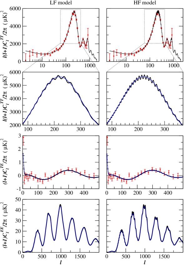
In those references, a detailed comparison of the trans-Planckian signal with the recently released high accuracy WMAP data has been performed. The main result is that, with the oscillations taken into account, it is possible to decrease the $\chi^{2}$ significantly. Instead of $\chi^{2}\simeq 1431$ for $1342$ degrees of freedom for the standard slow-roll power spectra, one now obtains $\chi^{2}\simeq 1420$ for $1340$ degrees of freedom, i.e. $\Delta\chi^{2}\simeq 10$ compared to WMAP one. The reason for such an important improvement of the $\chi^{2}$ is due to the presence of the oscillations which permit a better fit of the cosmic variance outliers at small scales. The main question is of course the statistical significance of this result. In Ref. MR1 ; MR2 , the so-called F-test has been used and indicates that the result is significant. However, it is clear that other statistical tests, a complete exploration of the parameter space and, of course, new data, should be used before one can really conclude that superimposed oscillations are really present in the CMBR multipole moments. A fair description of the present situation is that there seems to be a hint for an interesting feature in the CMBR data and that, maybe, this feature is a signature of very high energy physics (it is clear that the oscillations, if their presence is confirmed, could have another physical origin).

Finally, we would like to conclude by a comment on the back-reaction problem. This question is crucial for the consistency of the approach used before. It is clear that the energy density of the perturbations must be smaller or equal than that of the inflationary background. This leads to the condition $|x|\leq\sqrt{3\pi}m_{{}_{\rm Pl}}/M_{{}_{\rm C}}$ which amounts to

$$|x|\sigma_{0}\leq 10^{4}\times\frac{\sigma_{0}^{2}}{\sqrt{\epsilon}}\,.$$ (177)

It is important to emphasize that the above constraint is only a sufficient condition, but by no means, unless proved otherwise, a necessary condition. In general, this constraint is difficult to satisfy. Some of the best fits described above suffer from this back-reaction problem, see Ref. LLMU ; MR1 ; MR2 . In fact, the above formula expresses a generic difficulty of the trans-Planckian question, this difficulty being present regardless of the approach used in order to model the new physics. The presence of trans-Planckian corrections means the presence of particles (with respect to the standard vacuum) the energy density of which is very easily of the order of the background energy density. On the other hand, if we try to satisfy the back-reaction constraint then the signal very easily becomes tiny and, hence, non observable. A major advance, which would allow us to escape the previous vicious circle, would be to calculate explicitly the effect of the back-reaction. Unfortunately, for the moment, this is still an open question and more work is required to tackle this very important task.

References

- (1) A. Guth, Phys. Rev. D 23, 347 (1981).
- (2) A. Linde, Phys. Lett. B 108, 389 (1982); A. Albrecht and P. J. Steinhardt, Phys. Rev. Lett. 48, 1220 (1982); A. Linde, Phys. Lett. B 129, 177 (1983).
- (3) J. Martin, Proceedings of the XXIV Brazilian National Meeting on Particles and Fields, Caxambu, Brazil, (2004), astro-ph/0312492.
- (4) D. Lyth and A. Riotto, Phys. Rept. 314, 1 (1999), hep-ph/9807278.
- (5) A. Linde, Talk at the Nobel Symposium “Cosmology and String Theory”, (2003), hep-th/0402051.
- (6) M. Turner, Phys. Rev. D 28, 1243 (1983).
- (7) L. Kofman, A. Linde and A. Starobinsky, Phys. Rev. D 56, 3258 (1997), hep-ph/9704452.
- (8) V. F. Mukhanov, H. A. Feldman, and R. H. Brandenberger, Phys. Rep. 215, 203 (1992).
- (9) J. Stewart, Class. Quantum Grav. 7, 1169 (1990).
- (10) J. A. Bardeen, Phys. Rev. D 22, 1882 (1980).
- (11) J. Martin and D. J. Schwarz, Phys. Rev. D 57, 3302 (1998), gr-qc/970449.
- (12) R. Kerner, Gen. Rel. Grav. 9, 257 (1978).
- (13) D. H. Lyth, Phys. Rev. D 31, 1792 (1985).
- (14) L. P. Grishchuk, Zh. Eksp. Teor. Fiz 67, 825 (1974).
- (15) G. F. Smooth, et al., Astrophys. J. 396, L1 (1992).
- (16) P. de Bernardis, this volume.
- (17) R. K. Sachs and A. M. Wolfe, Astrophys. J. 147, 73 (1967).
- (18) M. Panek, Phys. Rev. D 49, 648 (1986).
- (19) C. Cohen-Tannoudji, J. Dupont-Roc and G. Grynberg, “Photons et atomes, Introduction a l’électrodynamique quantique”, Editions du CNRS, (1987).
- (20) E. Kolb and M. Turner, “The Early Universe”, Frontier in Physics, Perseus Publishing, (1990).
- (21) J. Martin and D. J. Schwarz, Phys. Rev. D 62, 103520 (2000), astro-ph/9911225; J. Martin, A. Riazuelo and D. J. Schwarz, Astrophys. J. 543, L99 (2000), astro-ph/0006392.
- (22) C. L. Bennet et al., Astrophys. J. Suppl. 148, 1 (2003), astro-ph/0302207; G. Hinshaw et al., Astrophys. J. Suppl. 148, 135 (2003), astro-ph/0302217; L. Verde et al., Astrophys. J. Suppl. 148, 195 (2003), astro-ph/0302218; H. V. Peiris et al., Astrophys. J. Suppl. 148, 213 (2003), astro-ph/0302225.
- (23) A. Albrecht, P. Ferreira, M. Joyce and T. Prokopec, Phys. Rev. D 50, 4807 (1994); D. Polarski and A. Starobinsky, Class. Quantum Grav. 13, 377 (1996).
- (24) L. P. Grishchuk and J. Martin, Phys. Rev. D 56, 1924 (1997), astro-ph/9702018.
- (25) A. Lewis, A. Challinor and A. Lasenby, Astrophys. J. 538, 473 (2000), astro-ph/9911177, http://camb.info; S. Leach, http://astronomy.sussex.ac.uk/ sleach/inflation/camb-inflation.html.
- (26) S. Leach and A. Liddle, Phys. Rev. D 68, 123508 (2003), astro-ph/0306305.
- (27) S. Dodelson, hep-ph/0309057.
- (28) J. Martin and R. H. Brandenberger, Phys. Rev. D 63, 123501 (2001), hep-th/0005209; R. H. Brandenberger and J. Martin, Mod. Phys. Lett. A 16, 999 (2001), astro-ph/0005432.
- (29) J. C. Niemeyer, Phys. Rev. D 63, 123502 (2001), astro-ph/0005533; A. Kempf, Phys. Rev. D 63, 083514 (2001), astro-ph/0009209; R. Easther, B. R. Greene, W. H. Kinney and G. Shiu, Phys. Rev. D 64, 103502 (2001), hep-th/0104102; R. Easther, B. R. Greene, W. H. Kinney and G. Shiu, Phys. Rev. D 67, 063508 (2003), hep-th/0110226; A. Kempf and J. C. Niemeyer, Phys. Rev. D 64, 103501 (2001), astro-ph/0103225; R. H. Brandenberger and P. M. Ho, Phys. Rev. D 66, 023517 (2002), hep-th/0203119; S. F. Hassan and M. S. Sloth, hep-th/0204110; F. Lizzi, G. Mangano, G. Miele and M. Peloso, JHEP 0206, 049 (2002), hep-th/0203099; U. H. Danielsson, Phys. Rev. D 66, 023511 (2002), hep-th/0203198; R. Easther, B. R. Greene, W. H. Kinney and G. Shiu, Phys. Rev. D 66, 023518 (2002), hep-th/0204129; G. L. Alberghi, R. Casadio and A. Tronconi, gr-qc/0303035; C. Armendáriz-Picón and E. A. Lim, hep-th/0303103.
- (30) M. Lemoine, M. Lubo, J. Martin and J. P. Uzan, Phys. Rev. D 65, 023510 (2002), hep-th/0109128.
- (31) J. Martin and R. H. Brandenberger, Phys. Rev. D 68, 063513 (2003), hep-th/0305161.
- (32) J. Martin and D. J. Schwarz, Phys. Rev. D 67, 083512 (2003), astro-ph/0210090.
- (33) W. Unruh, Phys. Rev. D 51, 2827 (1995).
- (34) S. Corley and T. Jacobson, Phys. Rev. D 54, 1568 (1996), hep-th/9601073; S. Corley, Phys. Rev. D 57, 6280 (1998), hep-th/9710075.
- (35) T. Jacobson, this volume.
- (36) J. Martin and C. Ringeval, Phys. Rev. D 69, 064406 (2004), astro-ph/0310382.
- (37) J. Martin and C. Ringeval, astro-ph/0402609.