On the Decoherence of Primordial Fluctuations During Inflation

Abstract:

We study the process whereby quantum cosmological perturbations become classical within inflationary cosmology. By setting up a master-equation formulation we show how quantum coherence for super-Hubble modes can be destroyed by its coupling to the environment provided by sub-Hubble modes. We identify what features the sub-Hubble environment must have in order to decohere the longer wavelengths, and identify how the onset of decoherence (and how long it takes) depends on the properties of the sub-Hubble physics which forms the environment. Our results show that the decoherence process is largely insensitive to the details of the coupling between the sub- and super-Hubble scales. They also show how locality implies , quite generally, that the decohered density matrix at late times is diagonal in the field representation (as is implicitly assumed by extant calculations of inflationary density perturbations). Our calculations also imply that decoherence can arise even for couplings which are as weak as gravitational in strength.

1 Introduction and Summary

Recent precision observations [1, 2, 3] of temperature fluctuations within the Cosmic Microwave Background (CMB) agree well [4] with the predictions made for them by inflationary models, according to which the Universe once underwent an accelerated expansion during its remote past [5]. According to the inflationary picture, the observed CMB temperature variations are seeded by tiny primordial density perturbations in the much earlier universe, perturbations which began as quantum fluctuations during the earlier inflationary epoch.

More precisely, within the inflationary picture the primordial density fluctuations derive from the quantum fluctuations, $\langle\phi(x)\phi(y)\rangle$, of the quantum inflaton field, $\phi$, whose dynamics drives the signature accelerated expansion. The success of the inflationary picture requires these quantum fluctuations to be converted into classical spatial variations in the energy density whose amplitude varies stochastically as one moves from one Hubble patch to another within the Universe during the much later recombination epoch.

At present, the classicalization of primordial perturbations is understood in terms of the properties of the quantum state into which the fluctuation fields evolve (see, for example [6, 7]). It is known that both scalar and tensor density fluctuations evolve during inflation into a particular kind of quantum state – one very similar to the squeezed state of quantum optics [8, 9]. In particular, quantum expectation values of products of fields in a highly squeezed state turn out to be identical to stochastic averages calculated from a stochastic distribution of classical field configurations, up to corrections which vanish in the limit of infinite squeezing [7, 10, 11]. Quantum autocorrelation functions like $\langle\phi(x)\phi(y)\rangle$ become indistinguishable from autocorrelations for $c$-number fields $\varphi(x)$ computed within a classical stochastic process, when computed in the limit of large squeezing.

Our purpose in this note is to describe what these analyses do not address: the decoherence process through which the initial quantum state evolves into the corresponding stochastic ensemble of field configurations. That is, we wish to understand how the density matrix, $\rho[\varphi(x),\varphi^{\prime}(y)]=\langle\varphi(x)|\rho|\varphi^{\prime}(y)\rangle$, for each of the various quantum fields, $\phi(x)$, evolves from an initially pure state,

$$\rho[\varphi(x),\varphi^{\prime}(y)]=\Psi[\varphi(x)]\Psi^{*}[\varphi^{\prime}(y)]\,,$$ (1.1)

describing the initial conditions (where $\Psi[\varphi(x)]=\langle\varphi(x)|\psi\rangle$), to a mixed state,

$$\rho[\varphi(x),\varphi^{\prime}(y)]=P[\varphi(x)]\,\delta[\varphi(x)-\varphi^{\prime}(y)]\,,$$ (1.2)

describing the later classical stochastic probability distribution for the field amplitudes. Such a transition is implicit in the standard predictions of inflationary implications for the CMB, and our goal is to understand to what extent these predictions might depend on the details of how this decoherence is achieved.

Decoherence is a much-studied process outside of cosmology, although not all of the conceptual issues have been resolved. In particular, the transition from pure to mixed state we seek typically arises whenever the degrees of freedom of interest interact with an ‘environment’ consisting of other degrees of freedom whose properties are not measured. The measured degrees of freedom can make a transition from a pure to a mixed state once a partial trace is taken over this environmental sector.

We are most interested in those modes which are responsible for the correlations which are observed in the CMB and in structure formation – modes which have only come within the Hubble scale relatively recently. We take the relevant decohering environment to consist of those modes having much shorter wavelength, which entered the Hubble scale much earlier and whose correlations are not directly visible in the sky. By borrowing techniques from atomic and condensed-matter physics we set up a master equation for the density matrix of the observed modes which allows us to robustly identify how these modes decohere provided only that ($i$) the environment is large enough to not be overly perturbed by the modes whose decoherence we follow; ($ii$) the interactions with the environment are weak; and ($ii$) the characteristic correlation time of fluctuations in the environment is much smaller than the timescales of interest to the decoherence process.

We use this formalism to identify how the decoherence depends on the properties of the short-wavelength modes which are assumed to make up the environment. Other authors have also examined the decoherence problem, often using the formalism of influence functionals [12] (see, for example [10, 13, 14, 15, 16, 17]). Unfortunately, the complexity of this formulation often forces calculations to be performed only for free fields, which couple to one another only by mixing in their mass or kinetic terms, leaving the uncertainty as to whether the results are restricted to the special choices which are made for calculational purposes. The main virtue of our treatment in terms of the master equation is that it allows us to identify the nature of the decoherence process in a controllable approximation which can encompass very general, realistic environment-system interactions.

Our analysis leads to the following results:

• We find that the quantity in the environment which controls the decoherence process is the autocorrelation function of the interaction Hamiltonian, $V(t)$, which couples the observed modes to the environment: ${\rm Tr\,}_{\rm env}[\rho\,\delta V(t)\,\delta V(t^{\prime})]$, where the trace is over the environmental sector, $\rho$ denotes the system’s density matrix and $\delta V(t)=V(t)-{\rm Tr\,}_{\rm env}[\rho\,V(t)]$ represents the fluctuations of $V(t)$ (in the interaction representation). More complicated dependence on the properties of the environment only arise at higher order in $V(t)$.

• We find that the generic situation is that the observed modes decohere into a density matrix of the form of eq. (1.2), which is diagonal when expressed in terms of field eigenstates. This basis typically plays a special role because locality usually dictates that the important interactions between the modes of interest and their environment are diagonal when written in this basis. This point has previously been emphasized in ref. [18]

• We show that the final stochastic probability distribution in eq. (1.2) is given in terms of the initial pure state by $P[\varphi(x)]=|\langle\varphi(x)|\psi\rangle|^{2}$, and thereby justify more precisely the standard arguments which implicitly use the classical stochastic field distribution which reproduces the computed initial quantum fluctuations of the inflaton.

• We find that short wavelength modes of the environment have the potential to decohere longer-wavelength modes, but need not do so. In particular they should not do so if the environment is prepared with its modes in their adiabatic vacua. It is this observation which explains why we are able to measure quantum states at all in the lab, given that there are always an enormous number of short-wavelength modes to which any given experiment does not have access.

• We find that for simple choices for the short-distance environment there is ample time for decoherence to occur during or after inflation, even if the modes of interest are coupled to the environment with gravitational strength. Since all modes couple gravitationally, this shows that decoherence is ubiquitous for modes produced during inflation which are now observable on the largest scales. In the special case that decoherence arises due to Planck-suppressed couplings between super-Hubble inflaton modes and thermal sub-Hubble modes after reheating, decoherence is only now beginning to occur for those modes which cross the horizon during the recombination epoch, raising the intriguing possibility that this might have observable implications.

We next present these results in more detail. We do so by first briefly reviewing our approach to decoherence with an emphasis on the limits of validity of our calculations. We then examine two candidate environments, both of which are known to exist in most inflationary scenarios: ($i$) the short-wavelength modes of the metric and inflaton themselves, during inflation and afterwards (for which we find our calculations break down, although we give arguments as to why decoherence from this source may be unlikely); and ($ii$) those short-wavelength modes which are the first to thermalize after inflation ends (for which we argue our calculations apply, and show that decoherence could reasonably occur in the time available).

Our purpose is not to argue that either of these sources must provide the dominant source of decoherence, but rather to argue that our calculational tools suffice to identify that environments exist which have sufficient time to decohere initial quantum fluctuations. Our hope is that these tools can be used to compare potential sources of decoherence, with a view to identifying those which are the most important and how the detailed features of decoherence depend on the nature of the environment assumed. In particular, we hope to find observational consequences of the decoherence process which might be possible to use to test further the inflationary paradigm for generating primordial density fluctuations. We group some of the details of the calculations into appendices.

2 Decoherence and Environments

The word ‘decoherence’ can mean a variety of things (see, for example, [19, 20] for extensive discussions), but for the present purposes we intend it to refer to the transition from a state which is initially pure — i.e. its density matrix can be written $\rho=|\psi\rangle\langle\psi|$, for some state-vector $|\psi\rangle$ — to a mixed state (for which no such state-vector exists). Our interest is in how long this transition takes, and in the form of the final mixed state to which the system is led. Once the final mixed state is obtained, its interpretation as a classical statistical ensemble is most simply found using the basis in which it is diagonal, since in this basis we have $\rho_{\rm red}={\rm Tr\,}_{\rm env}\rho=\sum_{n}p_{n}|n\rangle\langle n|$, with $0\leq p_{n}\leq 1$ denoting the classical probability of finding the system in state $|n\rangle$ [21].

Convenient diagnostics for determining the purity of the state represented by a density matrix $\rho$ are given by the basis-independent expressions: $\rho^{2}=\rho$ and ${\rm Tr\,}[\rho^{2}]=1$, either of which are satisfied if and only if the state described by $\rho$ is pure. The equivalence of these criteria for purity rely on the fact that density matrices are defined to be hermitian, positive semi-definite and satisfy ${\rm Tr\,}[\rho]=1$.

2.1 The Master Equation

We now set up a master equation which allows us to describe the pure-to-mixed transition quantitatively, and in a way which can be applied to a broad variety of choices for both the observable sector and the environment. Our presentation here follows closely that of ref. [22] (see also [12, 23] for alternative approaches). To do so we write the system’s Hilbert space to be the direct product of the observable sector, $A$, and the environment, $B$: ${\cal H}={\cal H}_{A}\otimes{\cal H}_{B}$, and write the total Hamiltonian governing the system as the sum $H=H_{A}+H_{B}+V$, where $H_{A}$ and $H_{B}$ describe the dynamics of the subspaces $A$ and $B$ in the absence of their mutual interactions, and $V$ is the interaction term which couples them.

For the applications of present interest we may also imagine the system starts off without any correlations between these two sectors, and so is described by an initial density matrix: $\rho(t=t_{0})=\varrho_{A}\otimes\varrho_{B}$. The presence of the interaction $V$ generates correlations between the two sectors as the system evolves; these correlations make a general description of their further evolution difficult. A great simplification is possible, however, if three conditions are satisfied [24, 25, 26]:

1. The interactions between sectors $A$ and $B$ are weak;

2. System $B$ is large enough not to be appreciably perturbed by its interactions with system $A$;

3. The correlation time, $\tau$, over which the autocorrelations $\langle\delta V(t)\,\delta V(t-\tau)\rangle_{B}$ are appreciably nonzero for the fluctuations of $V$ in sector $B$, are sufficiently short, $V\tau\ll 1$.

In this case the dynamics of system $A$ over times $t\gg\tau$ does not retain any memory of the correlations with $B$ since these only survive for much shorter times. This allows us to treat the evolution of $A$ in the presence of $B$ as a Markov process. What emerges is a picture wherein the interactions with $B$ simply provide a stochastic component to the evolution of sector $A$. From this picture, we can derive a master equation which describes how the environment $B$ affects the evolution of the density matrix describing sector $A$, and in particular how quickly sector $B$ leads to decoherence in system $A$.

It is convenient to work within the interaction representation, for which the time evolution of operators is governed by $H_{A}+H_{B}$ while the evolution of states is governed by $V$. We concentrate on obtaining an evolution equation for the reduced density matrix, $\rho_{A}(t)={\rm Tr\,}_{B}[\rho(t)]$, since this includes all of the information concerning measurements involving observables only in sector $A$. As Appendix A shows, writing the interaction Hamiltonian in terms of product basis of operators — $V=\sum_{j}A_{j}\otimes B_{j}$ — and using the three assumptions given above allows the derivation of the following master equation for $\rho_{A}(t)$:

$$\frac{\partial\rho_{A}}{\partial t}=i\Bigl{[}\rho_{A},A_{j}\Bigr{]}\langle B_{j}\rangle_{B}-\,\frac{1}{2}\,{\cal W}_{jk}\Bigl{\{}\Bigl{(}\rho_{A}A_{j}A_{k}+A_{j}A_{k}\rho_{A}-2A_{k}\rho_{A}A_{j}\Bigr{)}\Bigr{\}}\,.$$ (2.1)

where there is an implied sum over any repeated indices, and $\langle\cdots\rangle_{B}={\rm Tr\,}_{B}[(\cdots)\varrho_{B}]$ denotes the average over the initial (and unchanging) configuration of sector $B$. The assumption of a short correlation time, $\tau$, has been used here to write

$$\langle\delta B_{j}(t)\delta B_{k}(t^{\prime})\rangle_{B}={\cal W}_{jk}(t)\delta(t-t^{\prime})\,,$$ (2.2)

which defines the $O(\tau)$ coefficients ${\cal W}_{jk}^{*}={\cal W}_{kj}$.

The crucial observation is that the three assumptions listed above ensure that corrections to this equation are of order $(V\tau)^{3}$, where $\tau$ denotes the correlation time over which quantities like $\langle\delta V(t)\,\delta V(t+\tau)\rangle_{B}$ are appreciably nonzero. The use of perturbation theory to evaluate $\partial\rho_{A}/\partial t$ therefore requires only that $\tau$ be sufficiently short: $V\tau\ll 1$. However once eq. (2.1) is justified in this way, its solutions can be trusted even if they are integrated over times $t$ for which $Vt\gg 1$.

2.2 Local Interactions and Spatially-Small Fluctuations

We now specialize to the case of interest for field theory, where interactions are local. Suppose, then, that sector $A$ and $B$ interact through interactions of the local form:

$$V(t)=\int d^{3}x\;{\cal A}_{i}(x,t)\,{\cal B}_{i}(x,t)\,,$$ (2.3)

where there is an implied sum on $i$, ${\cal A}_{i}$ denotes a local functional of the fields describing the $A$ degrees of freedom, and ${\cal B}_{i}$ plays a similar role for sector $B$.

In the special case that the degrees of freedom in sector $B$ have very short correlation lengths, $\ell$, (as well as times, $\tau$), their influence on $\partial\rho_{A}/\partial t$ can be represented in terms of local ‘effective’ interactions. That is, suppose

$$\langle\delta{\cal B}_{i}(x,t)\,\delta{\cal B}_{j}(x^{\prime},t^{\prime})\rangle_{B}={\cal U}_{ij}(x,t)\,\delta^{3}(x-x^{\prime})\,\delta(t-t^{\prime})\,,$$ (2.4)

where ${\cal U}_{ij}^{*}={\cal U}_{ji}$ is a calculable local function of position which is of order $\ell^{3}\tau$. As is shown in Appendix A, under this assumption the master equation, eq. (2.1) becomes:

$$\frac{\partial\rho_{A}}{\partial t}=i\int d^{3}x\;\Bigl{[}\rho_{A},{\cal A}_{j}\Bigr{]}\,\langle{\cal B}_{j}\rangle_{B}-\frac{1}{2}\int d^{3}x\;{\cal U}_{jk}\Bigl{[}{\cal A}_{j}{\cal A}_{k}\rho_{A}+\rho_{A}{\cal A}_{j}{\cal A}_{k}-2{\cal A}_{k}\rho_{A}{\cal A}_{j}\Bigr{]}\,.$$ (2.5)

Notice that this equation trivially implies $\partial\rho_{A}/\partial t=0$ for any $\rho_{A}$ which commutes with all of the ${\cal A}_{j}$. Eqs. (2.1) and (2.5) are the main results in this section, whose implications we explore in detail throughout the remainder of the paper.

We remark that eqs. (2.2) and (2.4) are a fairly strong conditions, inasmuch as they exclude significant correlations along the entire light cone. In particular, they exclude the application of the master equations, (2.1) and (2.5), to situations where $\langle\delta{\cal B}_{j}(x,t)\delta{\cal B}_{k}(x^{\prime},t^{\prime})\rangle$ depends only on the proper separation, $s(x,t;x^{\prime},t^{\prime})$, between $(x,t)$ and $(x^{\prime},t^{\prime})$, such as when $B$ is prepared in a Lorentz-invariant vacuum (like the Bunch-Davies vacuum of de Sitter space).

2.3 Solutions

If all of the operators ${\cal A}_{i}(x,t)$ commute at equal times then the implications of eq. (2.5) are most easily displayed by taking its matrix elements in a basis of states $|\alpha\rangle_{t}$ for which the operators ${\cal A}_{i}(x,t)$ are diagonal: ${\cal A}_{i}(x,t)|\alpha\rangle_{t}=\alpha_{i}(x)|\alpha\rangle_{t}$ (for fixed $t$). With this choice we denote

$$\rho_{t}[\alpha,\tilde{\alpha}]={}_{t}\langle\alpha|\rho_{A}|\tilde{\alpha}\rangle_{t},$$ (2.6)

and so using the interaction-picture evolution $\partial_{t}|\alpha\rangle_{t}=-iH_{A}|\alpha\rangle_{t}$, we find

$$\frac{\partial\rho_{t}}{\partial t}[\alpha,\tilde{\alpha}] = (\partial_{t}\langle\alpha|)\rho_{A}|\tilde{\alpha}\rangle+\langle\alpha|\partial_{t}\rho_{A}|\tilde{\alpha}\rangle+\langle\alpha|\rho_{A}(\partial_{t}|\tilde{\alpha}\rangle)$$ (2.7)

$$= \langle\alpha|\partial_{t}\rho_{A}|\tilde{\alpha}\rangle+i\langle\alpha|[\rho_{A},H_{A}]|\tilde{\alpha}\rangle\,.$$

Notice that the last term in this equation combines with the term involving $\langle V\rangle_{B}$ in eq. (2.5) to give the combination $i\langle\alpha|[\rho_{A},H_{A}+\langle V\rangle_{B}]|\tilde{\alpha}\rangle$ in the evolution of the matrix element $\rho_{t}[\alpha,\tilde{\alpha}]$. Because these terms describe a Hamiltonian evolution they cannot generate a mixed state from one which is initially pure. For our present purposes of understanding decoherence we need follow only those terms of eq. (2.7) which are $O(V^{2})$ and which do not simply describe pure-state evolution.

The general solution to this equation is easily given in those circumstances for which the term involving $H_{A}$ is negligible, since in this case evaluating the matrix elements gives

$$\frac{\partial\rho_{t}}{\partial t}=-i\rho_{t}\int d^{3}z\Bigl{[}\alpha_{i}(z)-\tilde{\alpha}_{i}(z)\Bigr{]}\langle{\cal B}_{i}(z,t)\rangle_{B}$$

$$\qquad\qquad\qquad-\rho_{t}\int d^{3}z\Bigl{[}\alpha_{i}(z)-\tilde{\alpha}_{i}(z)\Bigr{]}\Bigl{[}\alpha_{j}(z)-\tilde{\alpha}_{j}(z)\Bigr{]}\,{\cal U}_{ij}(z,t)\,.$$

These equations are readily integrated to yield

$$\rho_{t}[\alpha,\tilde{\alpha}]=\rho_{t_{0}}[\alpha,\tilde{\alpha}]\,e^{-\Gamma-i\Sigma}\,,$$ (2.8)

where

$$\Sigma = \int_{t_{0}}^{t}dt^{\prime}d^{3}z\Bigl{[}\alpha_{i}(z)-\tilde{\alpha}_{i}(z)\Bigr{]}\langle{\cal B}_{i}(z,t^{\prime})\rangle_{B}$$ (2.9)

$$\Gamma = \int_{t_{0}}^{t}dt^{\prime}d^{3}z\Bigl{[}\alpha_{i}(z)-\tilde{\alpha}_{i}(z)\Bigr{]}\Bigl{[}\alpha_{j}(z)-\tilde{\alpha}_{j}(z)\Bigr{]}{\cal U}_{ij}(z,t^{\prime})\,.$$

This solution describes the evolution of the reduced density matrix over timescales for which the unperturbed evolution due to $H_{A}$ is negligible.

As expected, the mean-field term (involving $\langle{\cal B}_{i}\rangle_{B}$) only changes the phase of the initial pure state and so it may be neglected to the extent that only the transition from pure state to mixed is of interest. The same would be true for the $H_{A}$ terms in eq. (2.7) if $[H_{A},A_{i}]=0$. Otherwise $H_{A}+\langle V\rangle_{B}$ acts to evolve, but not to decohere, the initial pure state. By contrast, those terms involving the fluctuations ${\cal U}_{ij}$ cause the reduced density matrix to take the form of a classical Gaussian distribution in the $\{\alpha_{i}(x)\}$, whose time-dependent width is controlled by the local autocorrelation function ${\cal U}_{ij}$. Provided this width shrinks in time, at late times the system evolves towards a density matrix which is diagonal in the $|\alpha\rangle$ basis, with diagonal probabilities that are time-independent and set by the initial wave-function:

$$P_{t}[\alpha]\equiv\rho_{t}[\alpha,\alpha]=\rho_{t_{0}}[\alpha,\alpha]=\Bigl{|}\Psi_{t_{0}}[\alpha]\Bigr{|}^{2}\,.$$ (2.10)

Here $\Psi_{t_{0}}[\alpha]$ is the wave-functional for the initial pure state.

These solutions describe the decoherence of the initial state into the classical stochastic ensemble for the variables, $\{\alpha_{i}\}$, which diagonalize the interactions with the decohering environment. Since general considerations of locality typically require the interactions, ${\cal A}_{i}$ to be ultra-local polynomials of the fields, this shows that the classical distribution to which decoherence leads is generically an ensemble in field space, $\varphi(x)$ [18, 21], just as is implicitly assumed in standard calculations of inflationary perturbations.

3 Decoherence in Cosmology

We next apply the above formalism to inflationary cosmology, in order to identify potential sources of decoherence for those fluctuations whose influence is observed in CMB measurements.

3.1 Generalization to FRW Geometries

We start with a short discussion of how eq. (2.5) must be modified when applied to an expanding Friedmann, Robertson Walker (FRW) universe. We may do so either using co-moving time or conformal time, leading to physically equivalent results.

The starting point is the generalization of eq. (2.3) to curved space. If we take the interactions ${\cal A}_{i}$ and ${\cal B}_{i}$ to be Lorentz scalars, the insertion of a factor of the 3-metric’s volume element gives

$$V(t)=a^{3}(t)\int d^{3}x\;{\cal A}_{i}(x,t)\,{\cal B}_{i}(x,t)\,.$$ (3.1)

Keeping in mind that the delta function transforms as a tensor density, eq. (2.4) becomes

$$\langle\delta{\cal B}_{i}(x,t)\,\delta{\cal B}_{j}(x^{\prime},t^{\prime})\rangle_{B}=\left[\frac{{\cal U}_{ij}(x,t)}{a^{3}(t)}\right]\,\delta^{3}(x-x^{\prime})\,\delta(t-t^{\prime})\,,$$ (3.2)

where ${\cal U}(x,t)$ is also a Lorentz scalar. With these choices eq. (2.5) generalizes to:

$$\frac{\partial\rho_{A}}{\partial t}=ia^{3}\int d^{3}x\;\Bigl{[}\rho_{A},{\cal A}_{i}\Bigr{]}\,\langle{\cal B}_{i}\rangle_{B}$$

$$\qquad-\frac{a^{3}}{2}\int d^{3}x\;{\cal U}_{jk}\Bigl{[}{\cal A}_{j}{\cal A}_{k}\rho_{A}+\rho_{A}{\cal A}_{j}{\cal A}_{k}-2{\cal A}_{k}\rho_{A}{\cal A}_{j}\Bigr{]}\,.$$

The equivalent result in conformal time is obtained using the replacement ${\rm d}t=a\,{\rm d}\eta$.

3.2 Short-Wavelength Modes as Environment

For applications to inflationary predictions for the CMB we take sector $A$ to be comprised of those modes of the inflaton-metric system whose wavelength allows them to be visible within current measurements. In particular, we take $A$ to consist of the Mukhanov field [29, 30],

$$v=a\,\left[\delta\phi+\frac{\varphi^{\prime}}{{\cal H}}\psi\right]\,,$$ (3.4)

which describes the physically relevant combination of the inflaton fluctuation, $\delta\phi$, and the scalar metric fluctuation, $\psi$ (see Appendix B for more specific definitions). Here $a(\eta)$ denotes the background scale factor as a function of conformal time, $\eta$, for which ${\cal H}=a^{\prime}/a$, and $\varphi$ is the background inflaton configuration. Primes denote differentiation with respect to $\eta$. What makes this variable convenient is that its linearized evolution is governed by a flat-space, free-field action in the presence of a time-dependent mass, $m^{2}=-z^{\prime\prime}/z$:

$$S_{2}\,=\,\frac{1}{2}\int{d^{4}x\,\left[v^{\prime 2}-\gamma^{ij}\partial_{i}v\,\partial_{j}v+\left(\frac{z^{\prime\prime}}{z}\right)v^{2}\right]},$$ (3.5)

where $z=a\varphi^{\prime}/{\cal H}$ and $\gamma_{ij}$ is the spatial FRW metric (which we choose in what follows to be flat).

We must then make a choice for the decohering environment, sector $B$. A minimal choice for $B$ consists of the short-wavelength modes of the inflaton and metric fields themselves, since these modes and their mutual interactions are in any case required to exist by the assumed fluctuation-generating mechanism. In this section we explore the extent to which these interactions can suffice to decohere longer-distance inflaton fluctuations, given their very weak strength.

In particular we ask how the time-scale for decoherence depends on the physical parameters of this environment, in order to determine if sufficient time is available for decoherence to have been completed for those modes relevant to the CMB between horizon exit and re-entry. Our goal in so doing is not to argue that these are the most important sources of cosmological decoherence, but rather to show that the inflaton couples with sufficient strength in the early universe to plausibly have had enough time to have decohered before horizon re-entry.

Causality Issues

We have seen that the master equation derived above only applies if the environment’s correlation time, $\tau$, is much smaller than the times over which the system of interest evolves. Since the Hubble scale, $H$, sets the natural timescale for evolution in an expanding universe, this formalism is most naturally applied to situations where it is sub-Hubble modes ($k/a\gg H$) which decohere super-Hubble modes ($k/a\mathrel{\raise 1.29167pt\hbox{$<$\kern-8.50006pt\lower 4.30554pt\hbox{$\sim$}}}H$). Can this type of decoherence be consistent with causality?

At first sight one might think not, since there are general arguments [33] which restrict how much short-wavelength quantum fluctuations can modify background fields like $\langle\phi\rangle=\varphi$. However our interest in this paper is in how the system’s density matrix evolves between horizon exit and re-entry, and in particular how the transition occurs from a pure state to one that is mixed. But this is to do with the entanglement of short- and long-wavelength modes and the destruction of the phase coherence amongst the long-wavelength modes which arises once the short-distance modes are traced out. Since mean quantities like $\varphi$ are not changed by this decoherence, it is not constrained by considerations such as those of [33]. We believe our situation is closer to Einstein-Podolsky-Rosen experiments, for which entanglements between widely-separated electrons can give rise to seemingly nonlocal evolution of the system’s density matrix.

3.3 Decoherence After Reheating

We now must decide when to look for decoherence between the epoch when the observed modes leave the horizon during inflation, and their re-entry in the not-so-distant past (see Figure 1). We seek an instance when the short-wavelength modes are prepared in states for which the short-distance assumptions, eqs. (2.2) and (2.4), are satisfied.

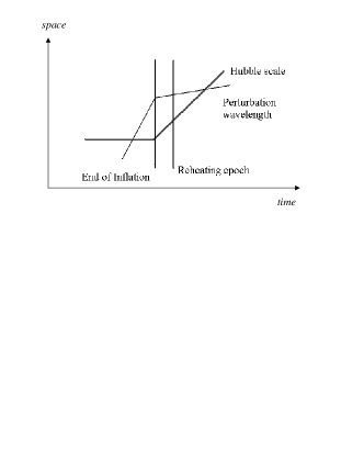
Figure 1: A cartoon of the evolution of the wavelength of a perturbation and the Hubble length vs time during inflation and afterwards. The vertical lines indicate the end of inflation, and the beginning of the subsequent reheating epoch.

The simplest such instance occurs after the reheating epoch. Reheating occurs once inflation ends and modes begin to re-enter the Hubble scale, since they can then acquire more complicated dynamics. Detailed studies indicate that under some circumstances this dynamics can lead to the reheating [31] and/or preheating [32] of the universe, giving rise to the thermal state which late-time Big Bang cosmology assumes.

Since thermal fluctuations can often satisfy the short-correlation assumptions, eqs. (2.2) and (2.4), we now examine whether a thermal bath of sub-Hubble modes can decohere the longer-wavelength, super-Hubble modes through their weak mutual self-interactions. Within this picture the first modes to thermalize would do so as in standard treatments, about which we have nothing new to say. Our interest is instead in how this nascent thermal (or other) mixed state acts to decohere those modes which only enter the Hubble scale much later, whose imprint we now see in the CMB. Since this type of decoherence cannot begin until after inflation ends, a key question is whether there is sufficient time over which to decohere the super-Hubble inflaton modes before they re-enter.

Decoherence Rates

In order to estimate whether there is sufficient time to decohere super-Hubble modes we require a simple model for the lowest-dimension inflaton/heat-bath interaction, which we take to have the form of eq. (2.3), with ${\cal A}=gv$ and where ${\cal B}$ is a local operator having engineering dimension (mass)^d, with $d>0$. On dimensional grounds the coupling $g$ then has dimension (mass)^3-d. With these assumptions the function ${\cal U}(x,t)$ defined by eq. (3.2) has dimension (mass)^2d-4. For later numerical estimates there are two cases of interest: ($i$) a dimension-4 (marginal) inflaton-bath coupling, for which $d=3$ and $g$ is dimensionless; and ($ii$) a dimension-5 interaction with $d=4$ and coupling $g=1/M$, for some large mass scale $M$.

Suppose now that the physics of sector $B$ is homogeneous in space and is characterized by a single mass scale, $\Lambda(t)$, which can be slowly evolving with time as the universe expands. For instance, $\Lambda(t)$ might be given by the temperature $T(t)$ if $B$ were described by a simple thermal state. Working in flat space we see that on dimensional grounds we can take

$$\langle{\cal B}(x,t)\rangle_{B}=c_{1}\,\Lambda^{d}(t)\quad\hbox{and}\quad{\cal U}(x,t)=c_{2}\,\Lambda^{2d-4}(t)\,,$$ (3.6)

where $c_{1}$ and $c_{2}$ are calculable dimensionless real numbers (which might also depend logarithmically on $\Lambda$, for large $\Lambda$). We imagine $c_{2}\geq 0$, which should be true for a broad class of choices for the environment (sector $B$).

Using these expressions, we then find

$$\langle V(t)\rangle_{B}=gc_{1}\,\Lambda^{d}(t)\,a^{3}(t)\int d^{3}x\;v(x,t)\,,$$ (3.7)

and

$$\frac{\partial\rho_{A}}{\partial t} = -i\Bigl{[}\langle V\rangle_{B},\rho_{A}\Bigr{]}$$

$$\quad-g^{2}\,c_{2}\,\Lambda^{2d-4}(t)\,a^{3}(t)\int d^{3}x\;\Bigl{[}v(x),\Bigl{[}v(x),\rho_{A}\Bigr{]}\Bigr{]}\,.$$

Evaluating this last equation within field eigenstates, $|V(x)\rangle_{t}$, and integrating over times short compared with $H^{-1}$ allows the neglect of the $H_{A}$ terms in $\partial_{t}\rho_{t}[V,\tilde{V}]$, leading to the integrated result

$$\rho_{t}[V,\tilde{V}]\approx\Bigl{|}\Psi_{t_{0}}[V]\Bigr{|}^{2}\,e^{-\Gamma-i\Sigma}\,,$$ (3.9)

with the decoherence rate governed by the quantity

$$\Gamma=g^{2}c_{2}\int_{t_{0}}^{t}dt^{\prime}\Lambda^{2d-4}(t^{\prime})\,a^{3}(t^{\prime})\int d^{3}z\Bigl{[}V(z)-\tilde{V}(z)\Bigr{]}^{2}\,.$$ (3.10)

Eq. (3.9) has the form of a Gaussian functional of $V(x)-\tilde{V}(x)$, whose interpretation can be estimated by evaluating it for configurations which extend over co-moving distances of order $L$ and whose amplitude is $V_{0}$. For such configurations we have

$$P_{t}(V_{0},\tilde{V}_{0})\sim P_{t_{0}}\exp\left[-\,\frac{L^{3}(V_{0}-\tilde{V}_{0})^{2}}{\sigma^{2}}\right]\,,$$ (3.11)

with a width, $\sigma$, which evolves with time according to

$$\frac{1}{\sigma^{2}} = g^{2}c_{2}\int^{t}_{t_{0}}dt^{\prime}\;\Lambda^{2d-4}(t^{\prime})\,a^{3}(t^{\prime})$$ (3.12)

$$= g^{2}c_{2}\int^{a}_{a_{0}}\frac{\hat{a}^{2}d\hat{a}}{H(\hat{a})}\;\Lambda^{2d-4}(\hat{a})\,.$$

To proceed we assume that $\Lambda$ evolves with time as does temperature. Then $\Lambda(a)=\Lambda_{0}(a_{0}/a)$ and so the width of the Gaussian density matrix acquires the time evolution

$$\frac{1}{\sigma^{2}} = g^{2}c_{2}\,\Lambda_{0}^{2d-4}a_{0}^{3}\int^{a/a_{0}}_{1}dx\;\left[\frac{x^{6-2d}}{H(x)}\right]$$ (3.13)

$$= \frac{1}{9-2d}\left(\frac{g^{2}c_{2}\,\Lambda_{0}^{2d-4}a_{0}^{3}}{H_{0}}\right)\left[\left(\frac{a}{a_{0}}\right)^{9-2d}-1\right]\,$$

where the last relationship assumes $H(a)=H_{0}(a_{0}/a)^{2}$, as is appropriate for a radiation-dominated universe.

The time-evolution of $\sigma$ differs qualitatively depending on whether $d\geq 5$ or $d\leq 4$. If $d\geq 5$ (corresponding to a dimension-6 or higher inflaton-matter interaction) then $1/\sigma^{2}$ saturates to $g^{2}c_{2}\,\Lambda_{0}^{2d-4}a_{0}^{3}/[(2d-9)H_{0}]$ as $a/a_{0}$ grows, indicating that for inflaton-matter couplings this weak the Gaussian maintains an essentially fixed width as the universe expands. By contrast, for $d\leq 4$ we find $\sigma$ shrinks to zero as $a/a_{0}$ grows without bound, indicating that couplings this strong lead at late times to a diagonal distribution in the $|V\rangle$ basis, corresponding to a stochastic statistical ensemble of classical field configurations, $V(x)$.

For the two cases of most interest (a dimension-5 inflaton-matter interaction with $d=4$ and $g=1/M$, or a dimension-4 interaction with $d=3$ and $g$ dimensionless) we find

$$\frac{L^{3}}{\sigma^{2}} = \left(\frac{\Lambda_{0}^{4}\,\ell_{0}^{3}}{M^{2}H_{0}}\right)\left(\frac{a}{a_{0}}\right)\quad\hbox{(if $d=4$)}$$ (3.14)

$$= \left(\frac{g^{2}\Lambda_{0}^{2}\,\ell^{3}(a)}{3H_{0}}\right)\quad\hbox{(if $d=3$)}\,,$$

for large $a/a_{0}$, where $\ell(a)=L\,a$ denotes the physical scale corresponding to the co-moving length $L$. These expressions show that $\sigma$ shrinks like $(a/a_{0})^{-1/2}$ or $(a/a_{0})^{-3/2}$ in these two cases as the universe expands.

We may also use these to estimate whether sufficient time can pass to decohere the modes of interest for CMB observations. To this end we evaluate the Gaussian distribution at the epoch of radiation-matter equality, for modes with amplitude $V_{0}-\tilde{V}_{0}\sim H_{\rm eq}=H(a_{\rm eq})$ and physical extent $\ell^{-1}(a_{\rm eq})\sim H_{\rm eq}$, starting with an initial pure state at the reheat epoch (for which $a_{0}=a_{\rm rh}$ and $H_{0}=H_{\rm rh}\sim T_{\rm rh}^{2}/M_{p}$). Using $H_{\rm eq}\sim T_{\rm eq}^{2}/M_{p}$, $a_{\rm eq}/a_{0}=T_{\rm rh}/T_{\rm eq}$, $\ell_{0}=\ell(a_{\rm eq})(a_{0}/a_{\rm eq})=H_{\rm eq}^{-1}(a_{0}/a_{\rm eq})$ and $H_{0}=H_{\rm eq}(a_{\rm eq}/a_{0})^{2}$ we have

$$\left(\frac{L^{3}H_{\rm eq}^{2}}{\sigma^{2}}\right)_{a=a_{\rm eq}} = \left(\frac{\Lambda_{0}^{4}}{M^{2}H_{\rm eq}^{2}}\right)\left(\frac{T_{\rm eq}}{T_{\rm rh}}\right)^{4}\sim\frac{M_{p}^{2}}{M^{2}}\qquad\hbox{(if $d=4$)}$$ (3.15)

and

$$\left(\frac{L^{3}H_{\rm eq}^{2}}{\sigma^{2}}\right)_{a=a_{\rm eq}} = \left(\frac{g^{2}\Lambda_{0}^{2}}{3H_{\rm eq}^{2}}\right)\left(\frac{T_{\rm eq}}{T_{\rm rh}}\right)^{2}\sim\frac{g^{2}M_{p}^{2}}{T_{\rm eq}^{2}}\qquad\hbox{(if $d=3$)}\,,$$ (3.16)

where the last approximate equalities use $\Lambda_{0}\sim T_{\rm rh}$.

Adequate decoherence requires $L^{3}(V-\tilde{V})^{2}/\sigma^{2}\gg 1$, and so we see that for $d=3$ this is true at radiation-matter equality for any $V-\tilde{V}\sim H_{\rm eq}$ given any reasonable choice for the dimensionless coupling $g$. It also occurs when $d=4$ provided only that the scale $M$ associated with the inflaton-matter coupling is smaller than the Planck scale. This shows that modes whose amplitudes differ in amplitude by as little as $H_{\rm eq}$ behave as if they have decohered by the time of radiation-matter equality.

Alternatively, we can ask for what epoch does the combination $L^{3}(V-\tilde{V})^{2}/\sigma^{2}$ become $O(1)$ for a mode with $V-\tilde{V}\sim H_{\rm eq}$ and $\ell(a_{\rm eq})\sim H^{-1}_{\rm eq}$. Using the above expressions we see this occurs when

$$\frac{a}{a_{0}} \sim \frac{M^{2}\,T_{\rm rh}}{M_{p}^{2}\,T_{\rm eq}}\quad\hbox{(if $d=4$)}$$

$$\frac{a}{a_{0}} \sim \frac{T_{\rm rh}}{(g^{2}M_{p}^{2}\,T_{\rm eq})^{1/3}}\quad\hbox{(if $d=3$)}\,.$$ (3.17)

If we demand that such modes decohere not long after the reheating epoch, such as when $a/a_{0}\sim N$ for $N$ not too much bigger than 1, then this requires

$$T_{\rm rh} \sim \left(\frac{NM_{p}^{2}\,T_{\rm eq}}{M^{2}}\right)\sim 10^{6}N\,\hbox{GeV}\left(\frac{10^{10}\,\hbox{GeV}}{M}\right)^{2}\qquad\hbox{(if $d=4$)}\,,$$ (3.18)

and

$$T_{\rm rh}\sim 10^{9}Ng^{2}\,\hbox{GeV}\quad\hbox{(if $d=3$)}\,.$$ (3.19)

For reheat temperatures of this order it is not necessary to trust the solution, eq. (3.9), for too long.

Finally, notice that if $M\sim M_{p}$ (when $d=4$) then we have $L^{3}(V-\tilde{V})^{2}/\sigma=O(1)$ for $V-\tilde{V}\sim H_{\rm eq}$ regardless of the reheat temperature, and so in this case all modes which differ in amplitude by an amount of order $H_{\rm eq}$ would be just beginning to decohere from one another as they re-enter the horizon. It is tempting to speculate that this might have measurable implications for the observed temperature fluctuations in the CMB.

3.4 Decoherence During Inflation?

We next explore the extent to which short-wavelength modes can decohere longer-wavelength modes during inflation itself, before a mixed environmental state has appeared. Our goal in this section is twofold. We first show why decoherence within this epoch cannot be reliably computed using the master-equation techniques presented within this paper — typically because of the failure of the short-time correlation assumptions, eqs. (2.2) and (2.4). We then argue why it should be unlikely that short-wavelength modes can decohere long-wavelength ones once a reliable method of calculation becomes possible.

3.4.1 Obstructions to Calculation

Since our interest for observations is in those modes having observational implications for the CMB, we again ask that sector $A$ consist of those long-wavelength modes of the Mukhanov field, $v$, which satisfy $k/a_{\rm he}\sim H$ at the epoch of horizon exit. All other modes of the field $v$ are not observed, and so can be lumped together and included into sector $B$ for the purposes of CMB observations. To this end it is useful to divide the field $v$ into a short- and long-wavelength part, $v=v_{l}+v_{s}$, where the long-wavelength modes, $v_{l}$, are those modes whose decoherence we wish to follow (sector $A$) and the short-wavelength modes, $v_{s}$, satisfy $k/a_{\rm he}\gg H$ and provide part of the environment over which we trace. (We ignore those modes of $v$ whose wavelengths are much longer than those which are observed, since their influence cannot be computed reliably using our methods of calculation.)

Since the environment satisfies $k/a_{\rm he}\gg H$, these modes start off in the ground state, $|0\rangle$, until a later epoch arises for which $k/a\sim H$, after which they start to become squeezed and so approach their Bunch Davies vacuum, $|B\rangle$. Of course, the environment (sector $B$) also includes the modes of all of the many other fields which are present in the high-energy theory besides the inflaton, many of which have masses $M\mathrel{\raise 1.29167pt\hbox{$>$\kern-8.50006pt\lower 4.30554pt\hbox{$\sim$}}}H$ and so for which all modes may be regarded as being ‘high-energy’ in comparison with the observable inflaton modes. For the present purposes we assume all of these modes to be in their Bunch-Davies vacuum state, which does not differ appreciably from the Minkowski vacuum to the extent that $k/a\gg H$ and/or $M\gg H$.

Consider, then, the following interaction lagrangian density

$${\cal L}_{\rm int}=-g\,{\cal B}[v_{h},\psi]\,v_{l}^{p}\,,$$ (3.20)

where $v_{l}$ denotes as above the observable inflaton modes, $p$ is some positive-integer power and ${\cal B}$ is some local functional of the inflaton’s short-wavelength modes, $v_{h}$, as well as of all other heavy fields, $\psi$. For instance, for the self-interactions of the inflaton we can use the estimate provided in Appendix B for the strength of its lowest-dimension self-interaction,

$${\cal L}_{\rm int}=-\xi\,v^{3}=-\xi(v_{h}^{3}+3v_{h}^{2}v_{l}+3v_{h}v_{l}^{2}+v_{l}^{3})\,,$$ (3.21)

with $\xi$ dominated (for a simple model of chaotic inflation) by the gravitational self-interactions, with strength

$$\xi\approx\pm\,\frac{48\,aH^{2}}{(2\epsilon)^{3/2}M_{p}}\,.$$ (3.22)

Here $H$ is the inflationary Hubble scale, and $\epsilon$ is the standard inflationary slow-roll parameter, $\epsilon=\frac{1}{2}(V^{\prime}/V)^{2}$. Since for a cubic interaction momentum conservation allows couplings between any three modes for which the sum $(k_{1}+k_{2}+k_{3})^{\mu}=0$, we see that cubic interactions can only couple very-short to very-long wavelength modes if two of the modes have short wavelengths and one has long. That is, only the term $-3\,\xi\,v_{h}^{2}v_{l}$ which can have nontrivial matrix elements and so participate in the mixing of very-long and very-short wavelength modes.

To compute the influence of sector $B$ for the decoherence of $v_{l}$ we must first estimate the relevant correlation function, $\langle\delta{\cal B}(x,t)\delta{\cal B}(x^{\prime},t^{\prime})\rangle$, and see whether it satisfies either of the short-correlation assumptions, eqs. (2.2) and (2.4). We must do so with the environment described by a pure squeezed state, which rapidly approaches the attractor corresponding to the Bunch-Davies vacuum, $|B\rangle$. For instance,starting with cubic inflaton self-interactions leads to the correlation function $\langle B|\delta v_{s}^{2}(x,t)\,\delta v_{s}^{2}(x^{\prime},t^{\prime})|B\rangle$, while an inflaton/heavy-field interaction of the form ${\cal L}_{\rm int}=g\psi\,v^{p}$ for a field with $\langle B|\psi|B\rangle=0$ would simply require the calculation of the Wightman function, $\langle B|\psi(x,t)\psi(x^{\prime},t^{\prime})|B\rangle$.

The main observation to be made is that when such a correlator is computed using the Bunch Davies vacuum, it generically does not satisfy the condition eq. (2.4). This is most easily seen for a heavy scalar field, $\psi$, of mass $m$, for which the calculation has been made explicitly [34] (see also [35]), with the result (in conformal time)

$$\langle B|\psi(x,\eta)\psi(x^{\prime},\eta^{\prime})|B\rangle=\left(\frac{1}{4}-\nu^{2}\right)\frac{H^{2}\sec(\pi\nu)}{16\pi}\,F\left[\frac{3}{2}+\nu,\frac{3}{2}-\nu,2;1+\frac{s^{2}}{4\eta\eta^{\prime}}\right]\,,$$ (3.23)

where $s^{2}(x,\eta;x^{\prime},\eta^{\prime})=(\eta-\eta^{\prime}-i\epsilon)^{2}-\delta_{jk}(x-x^{\prime})^{j}(x-x^{\prime})^{k}$, and $F[a,b,c;z]$ denotes the standard hypergeometric function. The complex parameter, $\nu$, is defined by $\nu^{2}=\frac{9}{4}-m^{2}/H^{2}$, and becomes pure imaginary in the limit $m>\frac{3}{2}\,H$. This expression does not have the $\delta$-correlated form of eq. (2.4) even in the limit $m\gg H$, because of the dependence on the separations in space and time only through the combination $s(x,\eta;x^{\prime},\eta^{\prime})$. The symmetries of de Sitter space ensure that this property is quite general for the correlations of scalar fields within their Bunch-Davies vacuum.

One might hope to press on despite of this by returning to first principles and simply using an expression like eq. (3.23) in the general result, eq. (A.7), of Appendix A. However since this equation is derived in perturbation theory, the result obtained for $\rho_{A}(t)$ in this way by integration generally cannot be trusted for times satisfying $Vt\mathrel{\raise 1.29167pt\hbox{$>$\kern-8.50006pt\lower 4.30554pt\hbox{$\sim$}}}O(1)$. For most applications this ensures that the result obtained cannot be used for any times of cosmological interest, reflecting the generic buildup of complicated correlations between sectors $A$ and $B$ as the sytem evolves. It is only because the short correlation-time assumption — $V\tau\ll 1$, or equivalently eq. (2.4) — makes the time-evolution problem into a Markov process that it is possible to trust the solutions to eq. (2.1) for $Vt\gg 1$.

3.4.2 Why Decoherence During Inflation is Unlikely

Although we see that it is difficult to compute decoherence effects during inflation within a controllable approximation, there are nevertheless strong reasons for doubting that interactions with short-wavelength field modes during inflation can decohere long-wavelength field modes. The reason hinges on the assumption that these short-wavelength modes are themselves in pure states, which in practice are well-approximated by the Bunch-Davies vacuum. This assumption is certainly a natural one to make for inflaton modes, given that the Bunch-Davies state is an attractor of the squeezing equations [9]. It is equally natural for the modes of other heavy fields (although it can be violated for some choices of scalar-field initial conditions [36]).

The point is that for short-wavelength modes the Bunch-Davies state is very close to the ordinary Minkowski vacuum, and so any decoherence which is generated by a short-wavelength mode during inflation is also likely to be present in flat space, in the absence of inflation. If it were true that having short-wavelength modes in their vacuum sufficed to decohere long-wavelength modes, it would be necessary to understand why we do not see the vacuum decohere around us all the time, and why quantum coherence is possible at all for the many low-energy states which have been studied throughout physics. Any convincing demonstration of decoherence during inflation by tracing out pure-state, short-wavelength modes must also explain why the same effect does not decohere long-wavelength modes within Minkowski space.

4 Discussion

In this paper we present a formalism within which it is possible to follow explicitly the development of decoherence within a system’s long-wavelength modes due to their interactions with various kinds of short-wavelength physics. The formalism relies for its validity on there being a large hierarchy between the correlation-time for fluctuations in the short-distance sector and the time-frame for evolution of the long-wavelength modes.

By applying this formalism to several possible choices for the short-distance environment we show that there is ample time during inflation for decoherence to occur between reheating and horizon re-entry for the modes of interest for CMB observations. We emphasize that our calculations do not yet establish what the most important source of decoherence might be for inflationary perturbations. In particular, we cannot compute with these tools how decoherence proceeds due to environments whose correlation times are not much shorter than the Hubble scale, or for short-wavelength modes prepared within their Bunch-Davies vacuum during inflation itself, although, we argue that decoherence during inflation by short-wavelength modes in their vacuum is unlikely, given the absence of such decoherence in non-cosmological situations.

Rather, our intent is merely to show that plausible sources could easily have sufficed to decohere the observed modes. Interestingly, if the decoherence is due to gravitational-strength interactions with the thermal (or other mixed) state produced during reheating, it could well be that the process is only just occurring for modes whose amplitudes differ by $O(H)$ as they re-enter the horizon near radiation-matter equality. If this should prove to be the most important source of decoherence we believe it would be worth exploring whether this might have observable consequences.

We argue that the decohered system tends to a final density matrix which is diagonal in a basis which also diagonalizes the relevant interaction Hamiltonian. On grounds of locality this is typically a basis for which the long-distance field operators themselves are diagonal. Since such a density matrix corresponds physically to the establishment of a stochastic distribution of classical field configurations, it is precisely the kind of late-time state which is implicitly assumed in standard calculations of the impact of inflationary fluctuations on the CMB.

Note Added:

While preparing this manuscript we discovered a paper, ref. [37], posted to the arXiv by one of our collaborators on this work. It describes an analysis which overlaps the one presented here on the calculation of the effects of decoherence by squeezed states during inflation. We believe that it differs in its conclusions due to errors in the calculations presented there, including (but not restricted to) the application of the master-equation formalism outside of its domain of validity.

Appendix A Interactions With a Fluctuating Environment

In this Appendix we summarize the formalism we use to determine the evolution of the density matrix for slow degrees of freedom interacting with an environment which contains fast fluctuations. We keep our exposition general, specializing to the case of interest at the end of the section.

A.1 General Formulation of the Problem

Our goal is to provide a general master equation which dictates the evolution of the density matrix of a system, $A$, of slow degrees of freedom which interacts with an environment, $B$, of faster modes. We do not follow any of the $B$ observables, and imagine that any correlations which the $B$ variables induce into the $A$ variables have correlation times which are very short compared with the time scale of the $A$-physics which is of interest. To this end we use a formalism which was developed for applications to physics in condensed-matter and atomic systems [24, 25, 26], but which has also seen service in describing neutrino evolution within complicated astrophysical environments [22].

Specifically, we imagine the system’s Hilbert space to be the direct product of the $A$ and $B$ Hilbert spaces, ${\cal H}={\cal H}_{A}\otimes{\cal H}_{B}$, and the total Hamiltonian to be described by the following sum

$$H=H_{0}+V=H_{A}\otimes I+I\otimes H_{B}+V\,,$$ (A.1)

where $H_{A}$ and $H_{B}$ are the Hamiltonians of the subspaces $A$ and $B$ in the absence of any interactions, and $V$ is the interaction term. In future we often suppress the presence of the unit operators, $I$. We also imagine the system starts off being described by a density matrix, $\rho$, for which there are no initial correlations between $A$ and $B$: $\rho(t=t_{0})=\varrho_{A}\otimes\varrho_{B}$.

In these circumstances a mean-field expansion allows practical progress, assuming that the correlation times, $\tau$, are small enough that $V\tau\ll 1$ for the matrix elements of interest. The mean-field expansion must be defined in terms of the time-evolution operator, since only in this case do the mean-field and fluctuation parts not interfere with one another. That is, if we consider the time-evolution operator in the interaction representation, then

$$\rho(t)=U(t)\,\rho(t=t_{0})\,U^{*}(t)$$ (A.2)

with

$$\frac{\partial U(t)}{\partial t}=-iV(t)\,U(t)\,,$$ (A.3)

where $V(t)=e^{iH_{0}t}\,V\,e^{-iH_{0}t}$.

Let us define the mean field $\overline{U}$ by

$$\overline{U}=\langle U\rangle_{B}={\rm Tr\,}_{B}[\rho U]\,,$$ (A.4)

where the trace is only over the states in sector $B$. Thus, $\overline{U}$ is an operator which acts in ${\cal H}_{A}$. Defining the fluctuation by $\Delta U=U-\overline{U}$, the exact time dependence of any $A$-sector observable, ${\cal O}_{A}$, can be written as

$$\langle{\cal O}_{A}\rangle(t) = {\rm Tr\,}\Bigl{[}\rho(t)\,{\cal O}_{A}\Bigr{]}$$

$$= {\rm Tr\,}\Bigl{[}U(t)\,\rho(t=t_{0})\,U^{*}(t)\,{\cal O}_{A}\Bigr{]}$$

$$= {\rm Tr\,}_{A}\Bigl{[}\overline{U}(t)\,\rho_{A}(t=t_{0})\,\overline{U}^{*}(t)\,{\cal O}_{A}\Bigr{]}$$

$$\qquad+{\rm Tr\,}\Bigl{[}\Delta U(t)\,\rho(t=t_{0})\,\Delta U^{*}(t)\,{\cal O}_{A}\Bigr{]}\,.$$

In the first term of the last line of this equation, $\rho_{A}$ is the reduced density matrix

$$\rho_{A}(t)={\rm Tr\,}_{B}[\rho(t)]\,,$$ (A.6)

which suffices to follow the time-dependence of any measurement only performed in sector $A$.

The last line of (A.1) also shows that defining the mean in terms of $U$ (rather than, say, $H$) guarantees that the time evolution of all observables decomposes into the sum of a mean evolution plus a fluctuation about this mean, with no cross terms involving both $\overline{U}$ and $\Delta U$. Indeed, this is the point of using $U$ (rather than $V$, say) when making the split between mean and fluctuating variables.

We now compute the differential evolution of $\rho_{A}(t)$ using perturbation theory, with $V$ being the perturbation. Expanding the exact evolution equation gives

$$\frac{\partial\rho_{A}}{\partial t}(t)=-i\Bigl{[}\overline{V}(t)\,\rho_{A}(t)-\rho_{A}(t)\,\overline{V}^{*}(t)\Bigr{]}$$ (A.7)

$$\qquad+\int_{t_{0}}^{t}d\tau\,{\rm Tr\,}_{B}\Bigl{[}\delta V(t)\,\rho(t)\,\delta V(\tau)+\delta V(\tau)\,\rho(t)\,\delta V(t)\Bigr{]}$$

$$\qquad+O(V^{3})\,.$$

In these expressions $\delta V=V-\overline{V}$ and $\overline{V}$ is defined in terms of $\overline{U}$ by

$$\overline{V}(t)=\left(i\frac{\partial\overline{U}}{\partial t}\right)\,\overline{U}^{-1}\,,$$ (A.8)

so

$$\overline{V}(t)=\langle V\rangle_{B}-i\int_{t_{0}}^{t}d\tau\,\langle\delta V(t)\delta V(\tau)\rangle_{B}+O(V^{3})\,.$$ (A.9)

Notice that $\overline{U}$ need not be unitary, because probability can scatter out of sector $A$ into sector $B$, or vice versa. Consequently, $\overline{V}$ need not be hermitian. However, an important special case for which $\overline{V}$ is unitary arises when the $B$ sector involves only states which are too heavy to be produced by the energy available in the $A$ sector, and the $B$ sector is prepared in its vacuum state: $\rho_{B}=|0\rangle_{B}{}_{B}\langle 0|$. The evolution of states in sector $A$ is guaranteed to be unitary in this case because there is no energy stored for release in sector $B$, and there is insufficient energy available in sector $A$ to excite states in sector $B$, and to thereby complicate the density matrix in this sector.

In the event that the system $B$ is large enough that its state is largely unchanged by the interactions with $A$, we can evaluate the right hand side of eq. (A.7) in terms of $\rho_{A}(t)$ by writing $\rho(t)\approx\rho_{A}(t)\otimes\varrho_{B}$, and thereby set up a differential equation which may be integrated to obtain the long-time behavior of $\rho_{A}(t)$. The point of this formulation is that this evolution can be trusted even over very long time scales, provided that the correlation time of system $B$ is sufficiently short.

Similarly, if we write the interaction Hamiltonian in the form $V(t)=A_{j}(t)\otimes B_{j}(t)$ (with an implied sum over ‘$j$’), and assume that the correlations in the fluctuations of $B_{j}$ are short-lived,

$$\langle\delta B_{j}(t)\delta B_{k}(t^{\prime})\rangle_{B}\equiv{\rm Tr\,}_{B}\Bigl{[}\varrho_{B}\delta B_{j}(t)\delta B_{k}(t^{\prime})\Bigr{]}={\cal W}_{jk}(t)\delta(t-t^{\prime})\,,$$ (A.10)

then we find

$$\overline{V}(t) = A_{j}(t)\langle B_{j}(t)\rangle_{B}-\frac{i}{2}\,{\cal W}_{jk}(t)A_{j}(t)A_{k}(t)$$

$$\hbox{and}\quad\overline{V}^{*}(t) = A_{j}(t)\langle B_{j}(t)\rangle_{B}+\frac{i}{2}\,{\cal W}_{jk}(t)A_{j}(t)A_{k}(t)\,.$$ (A.11)

These expressions use $\int_{t_{0}}^{t}dt^{\prime}\;f(t^{\prime})\delta(t-t^{\prime})=\frac{1}{2}\,f(t)$ and ${\cal W}^{*}_{jk}(t)={\cal W}_{kj}(t)$. The master evolution equation for $\rho_{A}(t)$ then is (neglecting $O(V^{3})$ terms)

$$\frac{\partial\rho_{A}}{\partial t}=i\Bigl{[}\rho_{A},A_{j}\Bigr{]}\langle B_{j}\rangle_{B}-\,\frac{1}{2}\,{\cal W}_{jk}\Bigl{\{}\Bigl{(}\rho_{A}A_{j}A_{k}+A_{j}A_{k}\rho_{A}-2A_{k}\rho_{A}A_{j}\Bigr{)}\Bigr{\}}\,.$$ (A.12)

A.2 Microscopic Fluctuations

We now specialize to the case where the degrees of freedom in sector $B$ also have very short wavelength, in which case their influence can be represented in terms of local interactions in the spirit of effective field theories. In this case the constraints of locality allow considerable simplification. Suppose, then, that sector $A$ and $B$ interact through a local interaction of the form:

$$V=\int d^{3}x\;\Bigl{[}{\cal A}_{j}(x,t)\otimes{\cal B}_{j}(x,t)\Bigr{]}\,,$$ (A.13)

where ${\cal A}_{j}$ denotes an ultra-local function of the fields describing the $A$ degrees of freedom, and ${\cal B}_{j}$ plays a similar role for sector $B$.

In terms of this interaction, the interaction potential, $\overline{V}$, is expressible (using the formulae given above) in terms of correlations of the variables ${\cal B}_{j}$. Using the assumption that these correlations in the $B$ sector are very short compared with the other scales of interest, we may write

$$\langle\delta{\cal B}_{j}(x,t)\,\delta{\cal B}_{k}(x^{\prime},t^{\prime})\rangle_{B}={\cal U}_{jk}(x,t)\,\delta^{3}(x-x^{\prime})\,\delta(t-t^{\prime})\,,$$ (A.14)

where the ${\cal U}_{jk}(x,t)={\cal U}^{*}_{kj}(x,t)$ are calculable local functions of position. Given this assumption, we have

$$\int_{t_{0}}^{t}dt^{\prime}\,\langle\delta V(t)\delta V(t^{\prime})\rangle_{B}=\frac{1}{2}\int d^{3}x\,{\cal A}_{j}{\cal A}_{k}\,{\cal U}_{jk}(x,t)\,.$$ (A.15)

and so we see that $\overline{V}(t)=\int d^{3}x\,\overline{{\cal V}}(x,t)$, with

$$\overline{{\cal V}}={\cal A}_{j}\langle{\cal B}_{j}(x,t)\rangle_{B}-\frac{i}{2}{\cal A}_{j}{\cal A}_{k}\,{\cal U}_{jk}(x,t)+O(V^{3})\,.$$ (A.16)

If probability and energy transfer can only flow into sector $B$ from sector $A$, then the matrix function ${\cal U}_{jk}$ is non-negative definite.

Using these expressions for the correlations of the energy density in the environment, we can write the master equation for $\rho_{A}(t)$ in the following way, accurate to second order in the coupling:

$$\frac{\partial\rho_{A}}{\partial t}=i\int d^{3}x\;\Bigl{[}\rho_{A},{\cal A}_{j}\Bigr{]}\,\langle{\cal B}_{j}\rangle_{B}-\frac{1}{2}\int d^{3}x\;{\cal U}_{jk}\Bigl{[}{\cal A}_{j}{\cal A}_{k}\rho_{A}+\rho_{A}{\cal A}_{j}{\cal A}_{k}-2{\cal A}_{k}\rho_{A}{\cal A}_{j}\Bigr{]}\,.$$ (A.17)

This is the result quoted as eq. (2.5) in the main text.

A.2.1 Example: Photons in a Thermal Fluid

An explicit example of practical interest to which the key assumption, eq. (A.14), applies is that of light propagating through an electrically neutral medium, for which sector $A$ consists of the photons and sector $B$ is the medium. Taking the photon-medium interaction to be given by

$${\cal L}_{\rm int}=eA_{\mu}J^{\mu}\,,$$ (A.18)

where $J^{\mu}$ is the electric-current operator, shows that we may take ${\cal A}=eA_{\mu}$ and ${\cal B}=J^{\mu}$. Provided the medium is electrically neutral and carries no net currents we then find $\langle J^{\mu}\rangle_{B}=0$, and eq. (A.14) becomes

$$\langle J^{\mu}(x,t)J^{\nu}(x^{\prime},t^{\prime})\rangle_{B}\approx\Pi^{\mu\nu}(x,t)\,\delta^{3}(x-x^{\prime})\delta(t-t^{\prime})\,,$$ (A.19)

where we follow conventional practice and use the notation $\Pi^{\mu\nu}$ (instead of ${\cal U}_{jk}$) for the current correlation function.

With these assumptions the effective photon lagrangian, eq. (A.16) becomes

$$\overline{\cal V}=-\frac{ie^{2}}{2}A_{\mu}A_{\nu}\Pi^{\mu\nu}(x,t)+O(V^{3})\,,$$ (A.20)

which shows that photon propagation through a medium is governed by the medium’s polarization tensor, $\Pi^{\mu\nu}$, with photon scattering being governed by fluctuations of the electric current within the medium. In the special case where the medium’s current fluctuations are due to thermal fluctuations in a rotationally-invariant fluid which is in local thermal equilibrium, then they have the form

$$\Pi^{\mu\nu}=\left(\begin{array}[]{cc}\pi_{1}&0\\ 0&\pi_{2}\,\delta^{ij}\end{array}\right)\,,$$ (A.21)

with local quantities, $\pi_{1}$ and $\pi_{2}$, which are calculable in terms of the local thermodynamic variables. If the temperature is much higher than the other relevant scales then we expect on dimensional grounds that $\pi_{a}=k_{a}\,T^{2}$, where $k_{1}$ and $k_{2}$ are calculable dimensionless constants, leading to a photon scattering rate which is of order $\Gamma\sim e^{2}T^{2}$. Ref. [22] shows that a similar analysis for neutrino propagation reproduces the standard results for neutrino scattering by a thermal bath.

A.3 Pure-to-Mixed Transitions

We next identify what features of the master equation play a role in making transitions from pure states to mixed states.

A pure state is defined by the condition that there exists a state vector, $|\psi\rangle$, for which the density matrix can be written $\rho_{A}=|\psi\rangle\langle\psi|$. This is a special case of the diagonal representation for $\rho_{A}$,

$$\rho_{A}=\sum_{n}p_{n}|n\rangle\langle n|\,,$$ (A.22)

for which $p_{n}=0$ for all $n\neq\psi$, and $p_{\psi}=1$ for $n=\psi$. This is equivalent to the basis-independent condition $\rho_{A}^{2}=\rho_{A}$. Since $\rho_{A}$ is non-negative definite and initially normalized, ${\rm Tr\,}[\rho_{A}]=1$, the coefficients $p_{n}$ satisfy $0\leq p_{n}\leq 1$ and so may be regarded as probabilities. In particular this implies $p_{n}^{2}\leq p_{n}$, with $p_{n}^{2}=p_{n}$ if and only if $p_{n}=0,1$. It follows that $\rho_{A}$ describes a pure state if and only if ${\rm Tr\,}[\rho^{2}_{A}]={\rm Tr\,}[\rho_{A}]=1$.

Motivated by these observations, we next use the master evolution equation, (A.12), to evaluate how ${\rm Tr\,}[\rho_{A}]$ and ${\rm Tr\,}[\rho_{A}^{2}]$ vary with time. As is simple to see,

$$\frac{\partial}{\partial t}\,{\rm Tr\,}[\rho_{A}] = i\langle B_{j}\rangle_{B}{\rm Tr\,}\Bigl{[}\rho_{A},A_{j}\Bigr{]}-\,\frac{1}{2}\,{\cal W}_{jk}{\rm Tr\,}\Bigl{\{}\Bigl{(}\rho_{A}A_{j}A_{k}+A_{j}A_{k}\rho_{A}-2A_{k}\rho_{A}A_{j}\Bigr{)}\Bigr{\}}$$ (A.23)

$$= 0\,,$$

and the rate for the pure-to-mixed transition is

$$\frac{\partial}{\partial t}\,{\rm Tr\,}[\rho^{2}_{A}] = {\rm Tr\,}\left[\rho_{A}\frac{\partial\rho_{A}}{\partial t}+\frac{\partial\rho_{A}}{\partial t}\rho_{A}\right]$$ (A.24)

$$= \Bigl{(}{\cal W}_{jk}+{\cal W}_{kj}\Bigr{)}\,{\rm Tr\,}\Bigl{[}\rho_{A}A_{j}\rho_{A}A_{k}\Bigr{]}-2{\cal W}_{jk}{\rm Tr\,}\Bigl{[}\rho_{A}^{2}A_{j}A_{k}\Bigr{]}\,.$$

Evaluating this for an initially pure state, $\rho_{A}(t_{0})=|\alpha\rangle\langle\alpha|$, then leads to

$$\left.\frac{\partial}{\partial t}\,{\rm Tr\,}[\rho^{2}_{A}]\right|_{t_{0}}=-2{\cal W}_{jk}(t_{0})\langle\alpha|\delta A_{j}\delta A_{k}|\alpha\rangle\,,$$ (A.25)

where $\delta A_{j}=A_{j}-\langle\alpha|A_{j}|\alpha\rangle$.

Appendix B Metric-Inflaton Perturbations

Before turning to explicit choices for the environment, we first pause to describe the observable sector (sector $A$) of interest for inflationary calculations. This allows us to identify the modes of interest for inflationary perturbations, and to estimate the size of their self-couplings.

B.1 Linearized Modes

For inflationary applications the observable system consists of those perturbations to the energy density which have wavelengths corresponding to those which are responsible for the observed temperature fluctuations in the CMB spectrum. Following standard practice we take these to be described by the appropriate combination of the scalar perturbations of the metric and the modes of the inflaton field, $\phi$, whose slow roll is responsible for the occurrence of inflation. Our description here draws extensively from the treatment in refs. [27, 28].

For single-field inflation the relevant dynamics is described by the action (using rationalized Planck units $M_{p}^{-2}=8\pi G=1$)

$$S=-\int d^{4}x\,\sqrt{-g}\left[\frac{1}{2}\,R+\frac{1}{2}\partial_{\mu}\phi\,\partial^{\mu}\phi+V(\phi)\right]\,.$$ (B.1)

Inflation can occur if the universe should enter a phase during which the total energy density is dominated by a slowly-rolling homogeneous expectation value, $\phi(t)$, whose kinetic energy is much smaller than its potential energy: $\frac{1}{2}\,\dot{\phi}^{2}\ll V(\phi)$. This can occur – given specific initial conditions – if the inflaton potential, $V(\phi)$, is chosen to be sufficiently flat. During inflation we take the space-time background to be

$${\rm d}s^{2}=-{\rm d}t^{2}+a^{2}(t)\,\gamma_{ij}\,{\rm d}x^{i}\,{\rm d}x^{j}\,,$$ (B.2)

where the Hubble scale, $H=\dot{a}/a$, is approximately constant and $\gamma_{ij}=\delta_{ij}$ denotes the spatial metric, which for simplicity we take to be flat.

The primordial fluctuations of relevance to the CMB within this picture are the quantum fluctuations of the inflaton field and of the scalar fluctuations of the metric. The wavelengths of these fluctuations are stretched exponentially during inflation, eventually to the size of the entire present-day observable universe.

Once formed, the evolution of the fluctuation is traced by linearizing the field equations about the inflationary background, using $\phi=\varphi+\delta\phi$ and $g_{\mu\nu}=\hat{g}_{\mu\nu}+\delta g_{\mu\nu}$, where $\varphi$ and $\hat{g}_{\mu\nu}$ represent the background inflationary solution to the equations of motion. Under these assumptions there is a gauge for which the scalar fluctuations of the metric can be written in terms of a scalar field, $\psi$, by

$$(\hat{g}+\delta g)_{\mu\nu}\,{\rm d}x^{\mu}{\rm d}x^{\nu}=a^{2}(\eta)\Bigl{(}-[1+2\psi(x,\eta)]\,{\rm d}\eta^{2}+[1-2\psi(x,\eta)]\,\gamma_{ij}{\rm d}x^{i}{\rm d}x^{j}\Bigr{)}\,.$$ (B.3)

We here switch to conformal time, defined by ${\rm d}t=a(\eta)\,{\rm d}\eta$, and ignore vector and tensor metric fluctuations since these are not yet relevant for CMB observations.

Only one combination of the two fields $\delta\phi$ and $\psi$ propagates independently, and within the linearized approximation this combination is most efficiently identified in terms of the variable [29, 30]

$$v=a(\eta)\,\left[\delta\phi+\frac{\varphi^{\prime}}{{\cal H}}\psi\right]\,,$$ (B.4)

where primes denote differentiation with respect to $\eta$ and ${\cal H}=a^{\prime}/a=Ha$ is the conformal-time Hubble scale. Expanding the action to quadratic order in $v$ gives:

$$S_{2}\,=\,\frac{1}{2}\int{d^{4}x\,\left[v^{\prime 2}-\gamma^{ij}\partial_{i}v\,\partial_{j}v+\left(\frac{z^{\prime\prime}}{z}\right)v^{2}\right]},$$ (B.5)

where $z=a\varphi^{\prime}/{\cal H}$. The utility of the variable $v$ follows because this action has canonical kinetic terms, and simply describes the evolution of a free scalar field with a time-dependent squared mass, $m^{2}=-z^{\prime\prime}/z$, propagating in flat spacetime. This makes its evolution and quantization comparatively straightforward to understand.

Writing the fluctuation this way shows that the evolution of the fluctuation amplitude depends crucially on the relative size of the mode wave-vector, $k$, and the ‘mass’ term, $-z^{\prime\prime}/z$. In particular, this evolution changes qualitatively depending on whether $k/a$ is larger or small than the Hubble scale $H$. What is important is the relative size of these two changes during the course of inflation and afterwards. During inflation the wavelength, $\lambda_{k}(t)=a(t)/k$, stretches while the Hubble length, $H^{-1}$ remains almost constant, and so the modes relevant to the later universe at some point leave the horizon by transiting to $\lambda>H^{-1}$ at the epoch of horizon exit, roughly 60 $e$-foldings before the end of inflation. After inflation the Hubble length grows faster than does $\lambda$, and so modes begin to re-enter the Hubble radius once inflation ends (see Fig. (1)). After re-entry these fluctuations are imagined to provide the primordial seeds which are responsible for the observed temperature fluctuations in the CMB. Between horizon exit and re-entry, while $k/a\ll H$, the mode amplitude satisfies $v_{k}^{\prime\prime}\approx(z^{\prime\prime}/z)v_{k}$ and so $v_{k}(\eta)\propto z(\eta)\propto a(\eta)$, corresponding to $\delta\phi$ being approximately frozen. The proportionality $z\propto a$ holds if the equation of state for the background geometry does not change in time, as we henceforth assume.

The time-evolution of the quantum state of the field, $v$, may be understood using the second-quantized Hamiltonian for the action $S_{2}$, which is

$$H_{A}={H}_{\rm free}-i\left(\frac{z^{\prime\prime}}{z}\right)\int{d^{3}{k}}\Bigl{(}a_{k}\,a_{-k}-\hbox{\rm h.c.}\Bigr{)}\,,$$ (B.6)

where ${H}_{\rm free}$ is the usual harmonic-oscillator Hamiltonian for each mode. Because the second term in this expression is time-dependent, it causes the energy eigenstates to evolve away from the adiabatic vacua, leading to the ‘squeezing’ for super-Hubble modes which satisfy $k/a\ll H$. Typically this evolution leads to an attractor solution, corresponding to the Bunch-Davies vacuum state. For sub-Hubble modes ($k/a\gg H$), by contrast, the second term in (B.6) is dominated by the first term, and so this state does not differ much from the ‘Minkowski’ ground state defined by $a_{k}|0\rangle=0$.

B.2 Coupling Strengths

For later use we next estimate the typical strength of the self-interactions amongst these linearized fluctuations. It suffices for our purposes to focus on cubic self-interactions of the general form

$${\cal L}_{\rm int}=-\xi\,v^{3}\,,$$ (B.7)

for which we wish to estimate $\xi$. Since $v$ is a linear combination of $\delta\phi$ and $\psi$, such couplings can potentially arise either as inflaton or as gravitational self-interactions. In this section we argue that the slow-roll requirement on the inflaton potential ensures that gravitational interactions provide the dominant cubic contribution.

Gravitational Self-Interactions

An estimate the size of cubic metric self-couplings is obtained by expanding the Einstein-Hilbert action to cubic order in $\psi$. Evaluating the Ricci scalar for the metric of eq. (B.3) and dropping derivatives of $\psi$ leads to

$$R=-\,\frac{6\,a^{\prime\prime}}{a^{3}(1+2\,\psi)\,}+\hbox{($\partial\psi$ terms)}\,,$$ (B.8)

and so the cubic term in the Einstein-Hilbert lagrangian density, ${\cal L}_{EH}=-\frac{1}{2}\,\sqrt{-g}\,R$, is

$${\cal L}_{3}=-24\,aa^{\prime\prime}\psi^{3}=-\,\frac{24a^{\prime\prime}}{a^{2}}\left(\frac{{\cal H}}{\varphi^{\prime}}\right)^{3}v^{3}\,,$$ (B.9)

where the last equality expresses the result in terms of the canonically-normalized variable obtained by dropping $\delta\phi$ from the definition of $v$: $\psi\sim[{\cal H}/(a\,\varphi^{\prime})]v=[H/(a\,\dot{\varphi})]v$.

Specialized to the near-de Sitter geometry appropriate during inflation we have $a^{\prime\prime}/a^{2}=2aH^{2}$ for constant $H$, related to the scalar potential by $3H^{2}\approx V$. Furthermore, ${\cal H}/\varphi^{\prime}=H/\dot{\varphi}\approx-3H^{2}/V^{\prime}\approx\pm(2\epsilon)^{-1/2}$, where $\epsilon=\frac{1}{2}(V^{\prime}/V)^{2}$ is the usual slow-roll parameter and we use the slow-roll condition $3H\dot{\varphi}\approx-V^{\prime}$. (When applied to $V$, primes here denote derivatives with respect to its argument, $\varphi$.) Eq. (B.9) then reduces to

$${\cal L}_{3}=-48\,a^{4}H^{2}\,\psi^{3}=\mp\left[\frac{48aH^{2}}{(2\epsilon)^{3/2}}\right]v^{3}\,,$$ (B.10)

where the upper (lower) sign applies if $\varphi^{\prime}>0$ ($<0$). Restoring $M_{p}=(8\pi G)^{-1/2}$, this represents a contribution to the cubic coupling which during inflation is of order

$$\xi_{g}\approx\pm\,\frac{48\,aH^{2}}{(2\epsilon)^{3/2}M_{p}}\,.$$ (B.11)

Inflaton Self-Couplings

We next compare the estimate of the cubic gravitational self-coupling just made with that obtained from the inflaton scalar potential. Expanding $V$ to cubic order in $\delta\phi$ leads to the following cubic interaction ${\cal L}_{3}=-\sqrt{-g}\,V^{\prime\prime\prime}(\varphi)(\delta\phi)^{3}$. Since this depends on the third derivative, its size depends somewhat on the kind of inflationary potential which is used. For instance, for a simple model of chaotic inflation, defined by a potential of the form $V=\lambda\phi^{4}$, with $\lambda$ a dimensionless coupling constant, we have

$${\cal L}_{3}=-4\lambda a^{4}\varphi(\delta\phi)^{3}=-4\lambda a\,\varphi\,v^{3}\,,$$ (B.12)

leading to the effective trilinear coupling constant $\xi_{\phi}=4\lambda a\,\varphi$.

How does this compare with the previously-computed gravitational estimate? Taking the ratio $\xi_{\phi}/\xi_{g}$ gives

$$\frac{\xi_{\phi}}{\xi_{g}}=\frac{4\,\lambda a\,\varphi\,}{\pm 48aH^{2}/[(2\epsilon)^{3/2}M_{p}]}=\pm\left[\frac{\lambda M_{p}\,\varphi}{12H^{2}}\right](2\epsilon)^{3/2}=\pm\,\frac{1}{4}\,\left[\frac{\sqrt{2\epsilon}\,M_{p}}{\varphi}\right]^{3}=-\,\frac{\epsilon^{3}}{32}\,,\\$$ (B.13)

where we use sign$\,\varphi^{\prime}=-\,$sign$\,\varphi$, and simplify using the expressions $3H^{2}M_{p}^{2}\approx V=\lambda\varphi^{4}$ and $2\epsilon=(V^{\prime}/V)^{2}=16(M_{p}/\varphi)^{2}$ which are obtained using the assumed inflaton potential. Since the existence of a slow roll requires $\epsilon\ll 1$ we see that it is the graviton self-coupling which dominates. In what follows we therefore use a cubic self-interaction with strength given by the gravitational self-coupling when computing decoherence.

B.3 Squeezed States

This Appendix briefly summarizes some of the useful properties of the Bunch-Davies attractor, as described in the squeezed-state language. Our description here follows that of ref. [9].

Since the evolution of the field $v$ whose evolution is governed by the Hamiltonian (B.6), the evolution of its ground state can be written $U|0\rangle$, where

$$U=S(r_{k},\Phi_{k})\,R(\Theta_{k})\,.$$ (B.14)

Here the operators $S$ and $R$ are defined by

$$S(r_{k},\Phi_{k}) = \exp\left[\frac{r_{k}}{2}\left(e^{-2i\Phi_{k}}a_{-k}a_{k}-\hbox{h.c.}\right)\right],$$

$$R(\Theta_{k}) = \exp\left[-i\Theta_{k}\Bigl{(}a^{*}_{k}a_{k}+a^{*}_{-k}a_{-k}\Bigr{)}\right]\,,$$ (B.15)

and $S(r_{k},\Phi_{k})$ defines the state’s squeezing, while $R(\Theta_{k})$ represents a rotation.

The parameters $r_{k}$, $\Phi_{k}$ and $\Theta_{k}$ are computable functions of conformal time, $\eta$, given an explicit inflationary scenario. An attractor solution for these parameters is given by [9]:

$$r_{k} = \sinh^{-1}\left(\frac{1}{2k\eta}\right)$$

$$\Phi_{k} = -\frac{\pi}{4}-\tan^{-1}\left(\frac{1}{2k\eta}\right)$$ (B.16)

$$\Theta_{k} = k\eta+\tan^{-1}\left(\frac{1}{2k\eta}\right)\,,$$ (B.17)

corresponding to the Bunch-Davies vacuum of de Sitter space.

References

-
[1]
C. L. Bennett et al.,
Astrophys. J. Suppl. 148 (2003) 1
[astro-ph/0302207];
D. N. Spergel et al. [WMAP Collaboration], Astrophys. J. Suppl. 148 (2003) 175 [astro-ph/0302209]. - [2] http://www.physics.ucsb.edu/ boomerang/
- [3] http://astro.uchicago.edu/dasi/
- [4] H. V. Peiris et al., “First year Wilkinson Microwave Anisotropy Probe (WMAP) observations: Implications for inflation,” Astrophys. J. Suppl. 148, 213 (2003) [astro-ph/0302225].
-
[5]
A. H. Guth, Phys. Rev. D23 (1981) 347;
A. D. Linde, Phys. Rev. B108 (1982) 389;
A. Albrecht and P. J. Steinhardt, Phys. Rev. Lett. 48 (1982) 1220. - [6] A. H. Guth and S. Y. Pi, Phys. Rev. D 32, 1899 (1985).
- [7] D. Polarski and A. A. Starobinsky, Class. Quant. Grav. 13, 377 (1996) [gr-qc/9504030].
- [8] L. P. Grishchuk and Y. V. Sidorov, Phys. Rev. D 42, 3413 (1990).
- [9] A. Albrecht, P. Ferreira, M. Joyce and T. Prokopec, Phys. Rev. D 50, 4807 (1994) [astro-ph/9303001].
- [10] C. Kiefer, D. Polarski and A. A. Starobinsky, Int. J. Mod. Phys. D 7, 455 (1998) [gr-qc/9802003].
- [11] J. Lesgourgues, D. Polarski and A. A. Starobinsky, Nucl. Phys. B 497, 479 (1997) [gr-qc/9611019].
- [12] R. P. Feynman and F.L. Vernon, jr., Ann. Phys. (N.Y.) 24, 118 (1963).
- [13] M. A. Sakagami, Prog. Theor. Phys. 79, 442 (1988).
- [14] R. H. Brandenberger, R. Laflamme and M. Mijic, Mod. Phys. Lett. A 5, 2311 (1990).
- [15] E. Calzetta and B. L. Hu, Phys. Rev. D 52, 6770 (1995) [gr-qc/9505046].
- [16] F. C. Lombardo and D. Lopez Nacir, Phys. Rev. D 72, 063506 (2005) [gr-qc/0506051].
- [17] L. P. Grishchuk and Y. V. Sidorov, Class. Quant. Grav. 6 (1989) L161.
- [18] C. Kiefer and D. Polarski, Annalen Phys. 7, 137 (1998) [gr-qc/9805014].
- [19] H. D. Zeh, Lect. Notes Phys. 538, 19 (2000) [quant-ph/9905004].
- [20] W. Zurek [quant-ph/0306072].
- [21] W. H. Zurek, Phys. Rev. D 24, 1516 (1981); J. P. Paz and W. H. Zurek, Phys. Rev. Lett. 82, 5181 (1999) [quant-ph/9811026], W. H. Zurek, S. Habib and J. P. Paz, Phys. Rev. Lett. 70, 1187 (1993).
- [22] C. P. Burgess and D. Michaud, Annals Phys. 256, 1 (1997) [hep-ph/9606295].
- [23] S. Chaturvedy and F. Shibata, Z. Phys. B35, 297; (1979); J. R. Anglin and W. H. Zurek, Phys. Rev. D 53, 7327 (1996) [quant-ph/9510021].
- [24] C. Cohen-Tannoudji, J. Dupont-Roc and G. Grynberg, Atom Photon Interactions, Wiley, New York, 1992.
- [25] V.F. Sears, Neutron Optics, Oxford University Press, 1989.
- [26] H. Haken, The Semiclassical and Quantum Theory of the Laser, in Quantum Optics: Proceedings of the Tenth Session of the Scottish Universities Summer School in Physics, 1969 ed. by S. M. Kay and A. Maitland, and references therein.
- [27] V. F. Mukhanov, H. A. Feldman and R. H. Brandenberger, Phys. Rept. 215, 203 (1992).
- [28] R. H. Brandenberger, Lect. Notes Phys. 646, 127 (2004) [hep-th/0306071].
- [29] V. F. Mukhanov, Sov. Phys. JETP 67, 1297 (1988) [Zh. Eksp. Teor. Fiz. 94N7, 1 (1988)].
- [30] V. N. Lukash, Sov. Phys. JETP 52, 807 (1980) [Zh. Eksp. Teor. Fiz. 79, (19??)].
- [31] A.D. Dolgov and A.D. Linke, Phys. Lett. B116 (1982) 329; W. Boucher and G.W. Gibbons, in The Very Early Universe, ed. by G.W. Gibbons, S.W. Hawking and S. SIklos, Cambridge 1983; A.A. Starobinsky, JETP Lett. 37 (1983) 66; R. Wald, Phys. Rev. D28 (1983) 2118; E. Martinez-Gonzalez and B.J.T. Jones, Phys. Lett. B167 (1986) 37; I.G. Moss and V. Sahni, Phys. Lett. B178 (1986) 159; M.S. Turner and L. Widrow, Phys. Rev. Lett. 57 (1986) 2237; L. Jensen and J. Stein-Schabes, Phys. Rev. D34 (1986) 329.
- [32] L. Kofman, A. Linde and A.A. Starobinsky, Phys. Rev. Lett. 73 (1994) 3195; D. Boyanovsky, J. de Vega, R. Holman, D.S. Lee and A. Singh, Phys. Rev. D51 (1995) 4419 [hep-ph/9507414]; Y. Shtanov, J. Traschen and R. Brandenberger, Phys. Rev. D51 (1995) 5438.
- [33] L.F. Abbott, J. Traschen and R.-M. Xu, Nucl. Phys. B296 (1988) 710; W. Boucher and J. Traschen, Phys. Rev. D37 (1988) 3522.
- [34] C. Schomblond and P. Spindel, Ann. Inst. Henri Poincaré 25A (1976) 67; T.S. Bunch and P.C.W. Davies, Proc. Roy. Soc. (London) A360 (1977) 117.
- [35] P. Candelas and D. J. Raine, Phys. Rev. D 12, 965 (1975); C.P. Burgess and C.A. Lutken, Phys. Lett. B153 (1985) 137.
- [36] C.P. Burgess, J.M. Cline, R. Holman and F. Lemieux, JHEP 0302 (2003) 048 [hep-th/0210233]; C.P. Burgess, J.M. Cline and R. Holman, JCAP 0310 (2003) 004 [hep-th/0306079].
- [37] P. Martineau, astro-ph/0601134.