Solving Stochastic Inflation for Arbitrary Potentials

Abstract

A perturbative method for solving the Langevin equation of inflationary cosmology in presence of backreaction is presented. In the Gaussian approximation, the method permits an explicit calculation of the probability distribution of the inflaton field for an arbitrary potential, with or without the volume effects taken into account. The perturbative method is then applied to various concrete models namely large field, small field, hybrid and running mass inflation. New results on the stochastic behavior of the inflaton field in those models are obtained. In particular, it is confirmed that the stochastic effects can be important in new inflation while it is demonstrated they are negligible in (vacuum dominated) hybrid inflation. The case of stochastic running mass inflation is discussed in some details and it is argued that quantum effects blur the distinction between the four classical versions of this model. It is also shown that the self-reproducing regime is likely to be important in this case.

I Introduction

Quantum effects play a crucial role during inflation. In particular, they are responsible for the self-reproducing behavior of the Universe also known as “eternal inflation” [1]. In this regime, the quantum fluctuations are so important that they can dominate the classical dynamics and, therefore, treating them properly becomes mandatory. Technically, this is a difficult task especially when it is necessary to take into account the backreaction of the quantum field on the geometry. Stochastic inflation [1, 2, 3, 4, 5, 6, 7] aims at providing a formalism where the previous difficulties can be partially circumvented. In the stochastic inflation approach, one is mainly interested in the evolution of a coarse-grained field, typically the original scalar field averaged over a Hubble patch, and the quantum effects are modeled by a stochastic noise originating from the small-scale Fourier modes. Consequently, the dynamics of the coarse-grained field is controlled by a Langevin equation. Then, endowed with a solution of this equation, one can compute the probability density function of the field and the various correlation functions.

Even if stochastic inflation simplifies the calculation of the quantum effects, the Langevin equation remains difficult to solve (without, of course, relying on numerical computations). The case without backreaction (in a de Sitter background) has been investigated in Ref. [8] where it has been shown that solutions for an arbitrary potential can be obtained. The case with backreaction is clearly much more complicated and something can be said about the solution only for very specific potentials. The usual approach is applicable when the inflaton potential is such that an exact solution exists for some power of the field. Then, in order to obtain the stochastic field itself and its various correlation functions, an expansion in terms of the coupling constant of the potential is performed. Explicit examples of this approach can be, for instance, found in Refs. [9, 10] and more recently in Ref. [11] and are briefly discussed in the following. The main point is that it is first necessary to obtain a solution to be subsequently able to perform the expansion. This is the reason why the applicability of the method is severely limited.

In this article, we present a method based on a perturbative expansion in the stochastic noise, the expansion being performed directly in the Langevin equation. As a consequence, our method does not require getting first a solution and, a priori, can be pushed to any order, the only limitation being the mathematical complexity of the obtained expressions. This represents a crucial advantage over the other approaches which allows us to treat analytically the case of an arbitrary potential with backreaction. It should be noticed that the idea to solve perturbatively the Langevin equation was put forward for the first time in Ref. [12]. In that reference, the method was used to compute the three-point correlation function of the Cosmic Microwave Background (CMB) anisotropy while, here, we use it in order to study the influence of the quantum effects on the behavior of the background inflaton. In particular, we show that, at second order, the calculation of the probability density function reduces to the calculation of a single quadrature. Moreover, the case where the volume effects are taken into account only requires the calculation of an additional integral. The method is then applied to various concrete cases, as the chaotic, new, hybrid and running mass inflationary models. In each case, the probability density function can be computed analytically and the volume effects evaluated exactly. This allows us to study the relevance of the quantum effects in those models. In particular, in the case of the running mass model, this is the first time that such an investigation is carried out.

Our paper is organized as follows. In the next section (Sec. II), we briefly review the basic equations of stochastic inflation. Then, in Sec. III, we present our method and compare it with the approaches known in the existing literature. We also show how to compute the probability density function, with or without the volume effects taken into account, directly from the Langevin equation without writing a Fokker-Planck equation. As already mentioned, we explicitly demonstrate that this calculation simply reduces to the calculation of a single quadrature. In Sec. IV, we briefly present the inflationary models the stochastic effects of which are computed in the subsequent section. In particular, we focus on the choice of the free parameters characterizing the corresponding potentials since their values are crucial in order to estimate the importance of the quantum effects. In Sec. V, we discuss and interpret our results for the cases of large field models, small field models, hybrid inflation and running mass inflation. To our knowledge, the calculation of the mean value and the variance of the coarse-grained field in the last three models was never done before (when the backreaction is taken into account). We end this article by some concluding remarks.

II Basic equations

In the Friedmann-Lemaître-Robertson-Walker (FLRW) Universe, the assumptions of homogeneity and isotropy allow us to write the metric in the simple form ${\rm d}s^{2}=-{\rm d}t^{2}+a^{2}(t)\delta_{ij}{\rm d}x^{i}{\rm d}x^{j}$, where $a(t)$ is the time-dependent scale factor and where we have assumed flat space-like sections. In such a space-time the evolution of an homogeneous scalar field $\phi(t)$, sourcing the metric evolution, is described by the Klein-Gordon equation

$$\ddot{\phi}+3H\dot{\phi}+V^{\prime}(\phi)=0\,,$$ (1)

where a dot means a derivation with respect to the cosmic time $t$ and a prime a derivation with respect to the scalar field $\phi$. This equation is coupled to the Friedmann equation for the scale factor

$$H^{2}\equiv\left(\frac{\dot{a}}{a}\right)^{2}=\frac{\kappa}{3}\left[\frac{\dot{\phi}^{2}}{2}+V(\phi)\right]\,,$$ (2)

where we have defined $\kappa\equiv 8\pi/m_{{}_{\mathrm{Pl}}}^{2}$, $m_{{}_{\mathrm{Pl}}}$ being the Planck mass.

During a phase of inflation, if the slow roll approximation is satisfied then the acceleration $\ddot{\phi}$ of the field is negligible compared to the friction term $3H\dot{\phi}$ and, at the same time, the kinetic energy $\dot{\phi}^{2}/2$ is small compared to the potential energy $V(\phi)$. This approximation considerably simplifies the equations describing the evolution of the system. These ones can now be re-written as

$$H^{2}(\phi)=\frac{\kappa}{3}V(\phi)\,,\quad\dot{\phi}+\frac{2}{\kappa}H^{\prime}\!(\phi)=0\,.$$ (3)

At the classical level, there is nothing more to say. Once we are given a potential $V(\phi)$, the above equations can be solved and the time evolution of the scale factor and of the inflaton field obtained.

The problem becomes much more complicated when the field $\phi$ is considered as a quantum operator. A first difficulty arises because quantizing a scalar in curved space-time is technically complicated for the case of an arbitrary potential (for an arbitrary potential, the Klein-Gordon equation is non-linear and one cannot Fourier expand the field and write an equation for a time-dependent mode function). A second (more fundamental) difficulty is to take into account the effect of the quantum scalar field on the geometry, i.e. the backreaction problem. Since the inflaton sources the Einstein equations, the Friedmann equation (taken literally) indicates that the geometry should also be quantized. Unfortunately, this quantum gravity regime is presently not known and the previous program cannot be carried out.

The stochastic formalism allows us to circumvent these difficulties. In the stochastic formalism [2], one is interested in the dynamics of a “coarse-grained” field $\varphi(t,{\bf x})$. This coarse-grained field is defined to be the spatial average of the ordinary field $\phi$ over a physical volume the size of which is typically larger than the Hubble radius $H^{-1}\equiv a/\dot{a}$. Therefore, $\varphi(t,{\bf x})$ basically contains the long-wavelength Fourier modes (i.e. those with comoving wavenumber such that $k<aH$) only.

The evolution of the coarse-grained field is still described by the Klein-Gordon equation (1) but a suitable random noise field $\xi(t)$, acting as a classical stochastic source term, should be added in order to take into account the effect of the quantum fluctuations. In the slow-roll approximation, the evolution of the coarse-grained field is thus governed by a first order Langevin-like differential equation which can be written as [1, 2, 3, 4, 5, 6, 7]

$$\dot{\varphi}+\frac{1}{3H}\frac{{\rm d}V}{{\rm d}\varphi}=\frac{H^{3/2}}{2\pi}\xi(t)\,,$$ (4)

where the noise field $\xi$ is defined in such a way that its mean and two-point correlation function simply read

$$\left\langle\xi(t)\right\rangle=0,\quad\left\langle\xi(t)\xi(t^{\prime})\right\rangle=\delta(t-t^{\prime})\,,$$ (5)

$\delta(z)$ being the Dirac distribution. The normalization of the correlation function is chosen in order to reproduce the ordinary result, $\left\langle\varphi^{2}\right\rangle=H^{3}t/(4\pi^{2})$, valid for a free field in de Sitter space-time.

It is at this point that the backreaction problem shows up. The standard assumption is that the Hubble parameter in Eq. (4) is only controlled by the coarse-grained field. Then, one needs to specify how $H$ depends on $\varphi$ and one naturally assumes that the Friedmann equation (in the slow-roll approximation) holds for the coarse grained quantities, namely

$$H^{2}(\varphi)\simeq\frac{\kappa}{3}V(\varphi)\,.$$ (6)

A direct consequence of the above equation is that the noise becomes multiplicative. The formalism briefly described previously also indicates that the coarse-grained field $\varphi$ now describes a Brownian motion for which the classical drift is modified by the quantum diffusion term. The main goal is to solve Eq. (4) since, endowed with the solution, we can then evaluate the probability density function of the coarse-grained field and/or various correlation functions.

III Solving stochastic inflation

III.1 Perturbative Method

As discussed above, the main purpose of this article is to present and study a method for solving the Langevin equation. This method was used for the first time in Ref. [12] for the calculation of CMB non-Gaussianities and in Ref. [13] in order to compute how the quantum effects affect the behavior of the quintessence field during inflation. Here, we develop the method in full generality including the calculation of the probability density function. The main idea is to consider the coarse-grained field $\varphi$ as a perturbation of the classical solution $\varphi_{\rm cl}$ (the classical solution is defined as the solution of the Langevin equation without the noise), $\varphi_{\mathrm{cl}}$ being supposed to be known. The corrections to $\varphi_{\rm cl}$ are obtained by adding successive terms of higher and higher powers in the noise, i.e.

$$\varphi(t)=\varphi_{\mathrm{cl}}(t)+\delta\varphi_{1}(t)+\delta\varphi_{2}(t)+\cdots\,,$$ (7)

where the term $\delta\varphi_{i}(t)$ depends on the noise at the power $i$. The equations of motion controlling the evolution of the term $\delta\varphi_{i}(t)$ are obtained by inserting the above expansion into the Langevin equation and by identifying the terms of same order. Expanding up to second order, we get two linear differential equations for $\delta\varphi_{1}$ and $\delta\varphi_{2}$, namely

$$\frac{{\rm d}\delta\varphi_{1}}{{\rm d}t}+\frac{2}{\kappa}H^{\prime\prime}(\varphi_{\rm cl})\delta\varphi_{1}=\frac{H^{3/2}(\varphi_{\rm cl})}{2\pi}\xi(t)\,,$$ (8)

and

$$\frac{{\rm d}\delta\varphi_{2}}{{\rm d}t} +\frac{2}{\kappa}H^{\prime\prime}(\varphi_{\rm cl})\delta\varphi_{2}=-\frac{H^{\prime\prime\prime}(\varphi_{\rm cl})}{\kappa}\delta\varphi_{1}^{2}$$

$$+\frac{3}{4\pi}H^{1/2}(\varphi_{\rm cl})H^{\prime}(\varphi_{\rm cl})\delta\varphi_{1}\xi(t)\,.$$ (9)

These equations are similar to Eq. (17) of Ref. [12]. The only difference is that, in the previous reference, the Langevin equation is written in term of the number of e-folds while, here, our time variable is the cosmic time. Since the above equations are linear, they can be solved by varying the integration constant. Straightforward manipulations lead to

$$\delta\varphi_{1}(t)=\frac{H^{\prime}\left[\varphi_{\rm cl}(t)\right]}{2\pi}\int_{t_{\mathrm{in}}}^{t}\!\!\mathrm{d}\tau\frac{H^{3/2}\left[\varphi_{\rm cl}(\tau)\right]}{H^{\prime}\left[\varphi_{\rm cl}(\tau)\right]}\xi(\tau)\,,$$ (10)

where we have assumed that the initial conditions are such that $\delta\varphi_{1}(t={t_{\mathrm{in}}})=0$. In the same manner, the solution for $\delta\varphi_{2}(t)$ can be easily obtained and reads

$$\delta\varphi_{2}(t)= -\frac{H^{\prime}}{\kappa}\int_{t_{\mathrm{in}}}^{t}\!\!\mathrm{d}\tau\frac{H^{\prime\prime\prime}}{H^{\prime}}\delta\varphi_{1}^{2}(\tau)$$

$$+\frac{3H^{\prime}}{4\pi}\int_{t_{\mathrm{in}}}^{t}\!\!\mathrm{d}\tau H^{1/2}\delta\varphi_{1}(\tau)\xi(\tau)\,.$$ (11)

As expected, $\delta\varphi_{1}$ is linear in the noise $\xi$ while $\delta\varphi_{2}$ is quadratic. Of course, the expansion could be pushed further and one could evaluate $\delta\varphi_{3}$, $\delta\varphi_{4}$ etc …using the same technique.

We are now in a position where the various correlation functions can be calculated exactly. Since $\delta\varphi_{1}$ is linear in the noise, its mean value obviously vanishes

$$\left\langle\delta\varphi_{1}\right\rangle=0\,.$$ (12)

This means that $\delta\varphi_{1}$ does not introduce any correction to the mean value of the coarse-grained field. As a matter of fact, $\delta\varphi_{1}$ directly contributes only to the variance of $\varphi$. Using the white noise correlation function given by Eq. (5), we obtain

$$\left\langle\delta\varphi_{1}^{2}\right\rangle=\frac{\kappa}{2}\left(\frac{H^{\prime}}{2\pi}\right)^{2}\!\!\int^{\varphi_{\mathrm{in}}}_{\varphi_{\rm cl}}\!\!\mathrm{d}\psi\left(\frac{H}{H^{\prime}}\right)^{3}\,.$$ (13)

We see that the calculation of the variance reduces to a simple quadrature. In order to calculate the correction to the mean value we must consider the mean of $\delta\varphi_{2}$. Using the fact that $\left\langle\delta\varphi_{1}(\tau)\xi(\tau)\right\rangle=H^{3/2}/(4\pi)$, we arrive at

$$\left\langle\delta\varphi_{2}\right\rangle= \,\frac{H^{\prime}}{2\pi m_{{}_{\mathrm{Pl}}}^{2}}\Bigg{\{}H^{\prime\prime}\!\int^{\varphi_{\mathrm{in}}}_{\varphi_{\mathrm{cl}}}\!\!\!\mathrm{d}\psi\left(\frac{H}{H^{\prime}}\right)^{3}$$

$$-\!\int^{\varphi_{\mathrm{in}}}_{\varphi_{\mathrm{cl}}}\!\!\!\mathrm{d}\psi\bigg{[}H^{\prime\prime}\left(\frac{H}{H^{\prime}}\right)^{3}-\frac{3}{2}\frac{H^{2}}{H^{\prime}}\bigg{]}\Bigg{\}}\,.$$ (14)

In this expression, the first term is nothing but the one given in (13), i.e. $\left\langle\delta\varphi_{1}^{2}\right\rangle$, while the second one can be evaluated exactly with the help of an integration by parts. This leads to

$$\left\langle\delta\varphi_{2}\right\rangle=\frac{H^{\prime\prime}}{2H^{\prime}}\left\langle\delta\varphi_{1}^{2}\right\rangle+\frac{H^{\prime}}{4\pi m_{{}_{\mathrm{Pl}}}^{2}}\Bigg{[}\frac{H_{\mathrm{in}}^{3}}{(H_{\mathrm{in}}^{\prime})^{2}}-\frac{H^{3}}{(H^{\prime})^{2}}\Bigg{]}\,.$$ (15)

Therefore, at second order in the noise, everything can be reduced to the calculation of a single quadrature, the one of Eq. (13). Before discussing the probability density function, we compare the method described above with what is already known in the literature.

III.2 Comparison with Other Methods

As already mentioned before, in order to treat the case with backreaction, various papers [9, 10] concentrate on very particular cases where the Langevin equation can be solved exactly (see also the recent article, Ref. [11], where the same method is used). The typical example of this procedure is the model described by a quartic potential, $V=3\lambda_{4}\varphi^{4}/(8\pi)$, $\lambda_{4}$ being a dimensionless coupling constant, for which the Langevin equation can be written as

$$\frac{{\rm d}}{{\rm d}t}\left(\frac{\varphi}{m_{{}_{\mathrm{Pl}}}}\right)+\frac{\sqrt{\lambda_{4}}}{2\pi}\varphi=\frac{\lambda_{4}^{3/4}m_{{}_{\mathrm{Pl}}}^{1/2}}{2\pi}\left(\frac{\varphi}{m_{{}_{\mathrm{Pl}}}}\right)^{3}\xi(t)\,.$$ (16)

This equation can be solved exactly because it takes the form of a Bernoulli equation after a change of variable. However, in this case, one does not obtain the coarse-grained field itself but rather some power of it, namely

$$\varphi^{-2}(t)=\varphi_{\mathrm{cl}}^{-2}(t)\left[1-\Psi(t)\right]\,,$$ (17)

where $\varphi_{\mathrm{cl}}(t)$ is the classical solution (which, in the slow-roll approximation, is known explicitly) and where the stochastic quantity $\Psi(t)$ is defined by

$$\Psi(t)\equiv\frac{\lambda_{4}^{3/4}m_{{}_{\mathrm{Pl}}}^{1/2}}{\pi}\int_{t_{\mathrm{in}}}^{t}{\rm d}\tau\left[\frac{\varphi_{\mathrm{cl}}(\tau)}{m_{{}_{\mathrm{Pl}}}}\right]^{2}\xi(\tau)\,,$$ (18)

which is a new dimensionless Gaussian noise with vanishing mean value and whose variance (and higher correlation functions) can easily be computed. Therefore, if one wants to obtain the field itself, it is necessary to take the inverse square root of the solution (17).

At this point, several remarks are in order. First, the only way to compute the coarse-grained field $\varphi$ and its various correlation functions is to expand $(1-\Psi)^{-1/2}$ in $\Psi$, that is to say in the coupling constant $\lambda_{4}$, and to truncate the expansion at some order (the series does not converge anyway). Thus, we see that, despite the fact that we have an exact solution, an expansion is still required in order to use Eq. (17) concretely. Second, one can show that the expansion in the coupling constant is equivalent to our expansion in the noise [13]. However, clearly, our method is more general because it is not restricted to the situation where an exact solution of the Langevin equation is available. This is because the expansion is directly performed in the Langevin equation rather than in its solution. The drawback of the method used in Refs. [9, 10] is clearly that it is first necessary to find a solution of the Langevin equation before the expansion can be taken. We will illustrate this last remark on the calculation of the criterion which determines when the self-reproducing regime becomes efficient (i.e. when the quantum fluctuations dominate the classical drift). In Ref. [11], using the model $V\propto\varphi^{4}$ for the reasons described before, the authors have recovered the standard result that this happens when the initial value of the inflaton is larger than $\varphi_{\mathrm{in}}\sim\lambda_{4}^{-1/6}m_{{}_{\mathrm{Pl}}}$. Using our formalism, we will derive this criterion for any model of the form $V\propto\varphi^{n}$, which would not have been possible with the method of Ref. [11].

Another possibility studied in the literature is the so-called scaling solutions method, see Ref. [14]. The idea is to perform a change of variable and to work in terms of a new stochastic process $\eta(\varphi)$ such that the Langevin equation takes the form ${\rm d}\eta/{\rm d}t={\cal F}(t;\eta)\xi(t)$, where ${\cal F}$ is a priori a complicated function of $\eta$. If $\eta$ is replaced by $\eta_{\mathrm{cl}}$ in ${\cal F}$, then the new Langevin equation becomes solvable. Therefore, one sees that this method bears some resemblance with the method investigated here. However, there also exists important differences. First, our method does not require any change of variable which is an advantage since, in general, the link between $\varphi$ and $\eta$ is quite complicated. Second, in the scaling method, there is no systematic expansion in the noise (in some sense one always works at first order) while in our method we can go to any order, the only limitation being mathematical complexity. Third, a saddle point approximation is used to estimate the effective dispersion while, in our case, following the calculations of the previous subsection, this can be done exactly. Fourth, it is difficult to evaluate the reliability of the scaling limit while we will discuss in a forthcoming article [15] how the accuracy of our method can be determined precisely. Finally, let us also stress that, in Ref. [14], only the cases of large field models and exponential potentials are considered (in principle, it would be possible to treat other models with the scaling method although it is unclear whether this would lead to analytical expressions for the probability density) while, here, we will also apply our method to the new, hybrid and running mass inflationary scenarios.

Finally, let us repeat that the method studied here is similar to the one used in Ref. [12] even if we apply it in a different context. In particular, the solution given by Eqs. (10) and (III.1) are identical to Eqs. (19) and (21) of Ref. [12], these formulas, however, being written in terms of the total number of e-folds rather than in terms of cosmic time. In Ref. [12], these results are applied to the calculation of the three-point correlation function of the CMB fluctuations while, in the present article, we use them, among others, in order to derive the probability density function of the background field.

To end this subsection, let us recall that more details on the other methods discussed here can be found in Ref. [13].

III.3 Probability Density Function

After having compared our approach with other formalisms, we now come back to the general method and show how one can calculate the single point probability distribution $P_{\rm c}(\varphi,t)$ of the coarse-grained field (also sometimes called $P_{\rm p}$ in the literature). Let us recall that $P_{\rm c}(\varphi,t)$ is the probability of the stochastic process to assume a given value at a given time in a single coarse-grained domain. Very often, this probability distribution is obtained from a Fokker-Planck equation. However, it can also be determined from [16]

$$P_{\rm c}(\varphi,t)=\left\langle\delta(\varphi-\varphi[\xi])\right\rangle\,.$$ (19)

where $\varphi[\xi]$ is the solution of the Langevin equation, and the mean value has to be evaluated with the functional probability distribution $\mathcal{P}[\xi]$ of the noise

$$\mathcal{P}[\xi]=\mathcal{N}_{0}\exp\left[-\frac{1}{2}\xi^{\rm T}\mathbf{C}^{-1}\xi\right],$$ (20)

with the normalization $\mathcal{N}_{0}$ simply being given by $\mathcal{N}_{0}=(\int\!\mathcal{D}\xi\,\mathrm{e}^{-\xi^{\rm T}\mathbf{C}^{-1}\xi/2})^{-1}$ and where we have introduced the definition $f^{\rm T}g\equiv\int\mathrm{d}\tau f(\tau)g(\tau)$. As one can see on the above expression, the noise probability distribution is Gaussian and correctly yields the noise correlation function $\left\langle\xi(t)\xi(t^{\prime})\right\rangle=\mathbf{C}(t,t^{\prime})$. In Eq. (19), the stochastic field will be given by our perturbative solution, namely $\varphi[\xi]=\varphi_{\mathrm{cl}}+\delta\varphi_{1}+\delta\varphi_{2}$. The first and second order corrections to the classical solution, which are linear and bilinear in the noise respectively, can also be written as $\delta\varphi_{1}=J^{\rm T}\xi$ and $\delta\varphi_{2}=\xi^{\rm T}\mathbf{A}\xi$, where the detailed definition of $J$ and $\mathbf{A}$ are given in Appendix A. Then, using the integral representation of the $\delta$ function, we get

$$P_{\rm c}(\varphi,t)=\frac{1}{2\pi}\int\mathrm{d}y\exp\left[iy\left(\varphi_{\mathrm{cl}}-\varphi\right)\right]{\cal N}_{0}\int\mathcal{D}\xi\,\exp\left[-\frac{1}{2}\xi^{\rm T}(\mathbf{C}^{-1}-2iy\mathbf{A})\xi+iyJ^{\rm T}\xi\right]\,.$$ (21)

In this expression the functional integration is a Gaussian integration involving the kernel $\mathbf{C}^{-1}-2iy\mathbf{A}$. Defining the new coefficient $\mathcal{N}_{y}=[\int\!\mathcal{D}\xi\,\mathrm{e}^{-\xi^{\rm T}(\mathbf{C}^{-1}-2iy\mathbf{A})\xi/2}]^{-1}$, the functional integration yields

$$P_{\rm c}(\varphi,t)=\frac{1}{2\pi}\int\mathrm{d}y\exp\left[iy\left(\varphi_{\mathrm{cl}}-\varphi\right)\right]\frac{{\cal N}_{0}}{{\cal N}_{y}}\exp\left[-\frac{1}{2}y^{2}J^{\rm T}(\mathbf{C}^{-1}-2iy\mathbf{A})^{-1}J\right]\,.$$ (22)

Then, generalizing the relation valid for two finite $n\times n$ matrices $\mathbf{M}$ and $\mathbf{N}$,

$$\frac{\displaystyle\int\mathrm{d}^{n}x\,\mathrm{e}^{-x_{i}M_{ij}x_{j}}}{\displaystyle\int\mathrm{d}^{n}x\,\mathrm{e}^{-x_{i}N_{ij}x_{j}}}=\sqrt{\frac{\det\mathbf{N}}{\det\mathbf{M}}}=\mathrm{e}^{-\mathrm{Tr}\ln\mathbf{N^{-1}}\mathbf{M}/2}\,,$$ (23)

to the continuous case [17], we can write the ratio of the two normalization coefficients as

$$\frac{\mathcal{N}_{0}}{\mathcal{N}_{y}} =\exp\left[-\frac{1}{2}\mathrm{Tr}\ln(\mathbf{1}-2iy\mathbf{AC})\right]\simeq\mathrm{e}^{iy\left\langle\delta\varphi_{2}\right\rangle}\,,$$ (24)

up to second order in the noise. Finally, if the argument of the second exponential in Eq. (22) is expanded in powers of the noise, then all the terms but $J^{\rm T}\mathbf{C}J=\left\langle\delta\varphi_{1}^{2}\right\rangle$ can be neglected. Evaluating the remaining ordinary integration over $y$ we get the normalized Gaussian distribution

$$P_{\rm c}(\varphi,t)=\frac{1}{\sqrt{2\pi\!\left\langle\delta\varphi_{1}^{2}\right\rangle}}\exp\!\left[-\frac{(\varphi-\varphi_{\mathrm{cl}}-\left\langle\delta\varphi_{2}\right\rangle)^{2}}{2\left\langle\delta\varphi_{1}^{2}\right\rangle}\right]\,.$$ (25)

This distribution is centered over the mean value $\left\langle\varphi\right\rangle\simeq\varphi_{\mathrm{cl}}+\left\langle\delta\varphi_{2}\right\rangle$ with variance $\left\langle\delta\varphi_{1}^{2}\right\rangle$. The above equation is one of the main result of this article. In order to evaluate $P_{\rm c}$ only the integration (13) is necessary which illustrates the power of the perturbative method.

III.4 Volume Effects

If we want to investigate the evolution of the probability distribution of the field when spatially averaged over the entire Universe (and not only in the single domain) we must take into account the volume effects. These are due to the fact that the size of each homogeneous domain depends on the value of the field within the domain itself, and we expect larger domains to give a more important contribution to the average over space. The value of each field-dependent quantity must thus be weighted with the physical volume $a^{3}(\varphi)=\exp[3\int{\rm d}\tau H(\varphi)]$. Therefore, the normalized probability distribution accounting for volume effects can be obtained from

$$P_{\rm v}(\varphi,t)=\frac{\left\langle\delta(\varphi-\varphi[\xi])\,\mathrm{e}^{3\!\int\mathrm{d}\tau H(\varphi[\xi])}\right\rangle}{\left\langle\mathrm{e}^{3\!\int\mathrm{d}\tau H(\varphi[\xi])}\right\rangle}\,.$$ (26)

In order to compute this new distribution function, we expand perturbatively $H(\varphi[\xi])$ up to second order in the noise,

$$H(\varphi[\xi])=H_{\mathrm{cl}}+H^{\prime}_{\mathrm{cl}}(\delta\varphi_{1}+\delta\varphi_{2})+\frac{H^{\prime\prime}_{\mathrm{cl}}}{2}\delta\varphi_{1}^{2}\,,$$ (27)

and write the first order term appearing in the argument of the exponential in Eq. (26) as $\int_{t_{\mathrm{in}}}^{t}\mathrm{d}\tau H^{\prime}(\tau)\delta\varphi_{1}(\tau)\equiv I^{\rm T}\xi$ while the second order ones take the form $\int_{t_{\mathrm{in}}}^{t}\mathrm{d}\tau\left[H^{\prime}(\tau)\delta\varphi_{2}(\tau)+H^{\prime\prime}(\tau)\delta\varphi_{1}^{2}/2\right]\equiv\xi^{\rm T}\mathbf{B}\xi$.

Then, one can repeat the calculations performed in the previous subsection and we obtain the following expression for the volume weighted distribution function

$$P_{\rm v}(\varphi,t)=\frac{1}{2\pi\left\langle a^{3}(\varphi)\right\rangle}\int\mathrm{d}y\exp\left[iy\left(\varphi_{\mathrm{cl}}-\varphi\right)\right]{\cal N}_{0}\int\mathcal{D}\xi\,\exp\left[-\frac{1}{2}\xi^{\rm T}(\mathbf{C}^{-1}-2iy\mathbf{A}-6\mathbf{B})\xi+\left(iyJ^{\rm T}+3I^{\rm T}\right)\xi\right]\,.$$ (28)

This is again a Gaussian integration but with the modified kernel $\mathbf{C}^{-1}-2iy\mathbf{A}-6\mathbf{B}$ where the term $-6\mathbf{B}$ is a new contribution that accounts for the volume effects. These volume effects also manifest themselves in the term linear in the noise (i.e. the term proportional to $I$). Following the same steps as before, we define the new normalization $\mathcal{N}^{\prime}_{y}=\left[\int\!\mathcal{D}\xi\,\mathrm{e}^{-\xi^{T}(\mathbf{C}^{-1}-2iy\mathbf{A}-6\mathbf{B})\xi/2}\right]^{-1}$ and evaluate the functional integral. We obtain

$$P_{\rm v}(\varphi,t)=\frac{1}{2\pi\left\langle a^{3}(\varphi)\right\rangle}\int\mathrm{d}y\exp\left[iy\left(\varphi_{\mathrm{cl}}-\varphi\right)\right]\frac{{\cal N}_{0}}{{\cal N}^{\prime}_{y}}\exp\left[\frac{1}{2}(iyJ^{\rm T}+3I^{\rm T})\left(\mathbf{C}^{-1}-2iy\mathbf{A}-6\mathbf{B}\right)^{-1}(iyJ+3I)\right]\,.$$ (29)

As in the previous case, the functional inverse of the modified kernel $(\mathbf{C}^{-1}-2iy\mathbf{A}-6\mathbf{B})^{-1}$ simply reduces, up to second order, to $\mathbf{C}$.

We must now evaluate the denominator. Exactly in the same way as before, this term becomes

$$\left\langle a^{3}(\varphi)\!\right\rangle={\cal N}_{0}\!\!\int\!\mathcal{D}\xi\exp\!\left[-\frac{1}{2}\xi^{\rm T}\!(\mathbf{C}^{-1}\!\!\!-6\mathbf{B})\xi+3I^{\rm T}\!\xi\right]\!,$$ (30)

and the functional integration yields $\left\langle a^{3}(\varphi)\right\rangle\simeq(\mathcal{N}_{0}/\mathcal{N}^{\prime}_{0})\exp\left(9I^{\rm T}\mathbf{C}I/2\right)$, where $\mathcal{N}^{\prime}_{0}$ is a new normalization coefficient the explicit expression of which we do not give here for simplicity. Then, we insert this last expression in Eq. (29). As expected the terms ${\cal N}_{0}$ cancels out. Moreover, when evaluating the ratio $\mathcal{N}^{\prime}_{0}/\mathcal{N}^{\prime}_{y}$, the contributions of the terms describing the volume effects (those involving $\mathbf{B}$) also cancel out at second order and we get $\mathcal{N}^{\prime}_{0}/\mathcal{N}^{\prime}_{y}\simeq\mathrm{e}^{iy\left\langle\delta\varphi_{2}\right\rangle}$ as before. Putting everything together, we obtain the final result

$$P_{\rm v}(\varphi,t)=\frac{1}{\sqrt{2\pi\!\left\langle\delta\varphi_{1}^{2}\right\rangle}}\exp\!\left[-\frac{\left(\varphi-\left\langle\varphi\right\rangle-\!3I^{\rm T}\!\!J\right)^{2}}{2\left\langle\delta\varphi_{1}^{2}\right\rangle}\right],$$ (31)

where $\left\langle\varphi\right\rangle\!=\varphi_{\mathrm{cl}}+\left\langle\delta\varphi_{2}\right\rangle$ is the usual mean value.

This expression should be compared with Eq. (25). The variance of the resulting Gaussian probability distribution is thus unchanged, while the volume-weighted mean value $\left\langle\varphi\right\rangle_{\rm v}=\left\langle\varphi\right\rangle+3\,I^{\rm T}\!J$ gets the extra correction

$$3\,I^{\rm T}\!J=3\!\int_{t_{\mathrm{in}}}^{t}\!\mathrm{d}\tau H^{\prime}(\tau)\left\langle\delta\varphi_{1}(t)\delta\varphi_{1}(\tau)\right\rangle\,.$$ (32)

So far, the calculation of the volume effects, in particular Eqs. (31) and (32), do not rely on the slow-roll approximation. However, if this approximation is satisfied, then the volume contribution can be easily calculated for a generic potential. We obtain

$$3I^{\rm T}\!J=\frac{12H^{\prime}}{m_{{}_{\mathrm{Pl}}}^{4}}\!\int_{\varphi_{\mathrm{cl}}(t)}^{\varphi_{\mathrm{in}}}\!\!\mathrm{d}\psi\frac{H^{4}}{(H^{\prime})^{3}}-12\pi\frac{H}{H^{\prime}}\frac{\left\langle\delta\varphi_{1}^{2}(t)\right\rangle}{m_{{}_{\mathrm{Pl}}}^{2}}\,.$$ (33)

Therefore, we see that the calculation of the volume effects only requires the computation of one additional quadrature.

IV Inflationary models

In this section, we briefly present the inflationary models to which our method is applied in the next section. In particular, we carefully discuss the choice of the free parameters characterizing those models since their numerical values turn out to be crucial in order to estimate the importance of the stochastic effects.

IV.1 Generalities

We adopt a parameterization of $V(\phi)$ suitable for describing different types of inflationary models, and we write the potential as

$$V(\varphi)=M^{4}\!\left[a+b\left(\frac{\varphi}{\mu}\right)^{\!\!n}\right]\,,$$ (34)

where $a=0,1$ and $b=\pm 1$ according to the case under consideration, while $M$, $\mu$ and $n$ (with $n\geq 2$) are free parameters. If $a=0$ and $b=1$ we have monomial potentials describing chaotic inflation [18], also commonly known as “large field models” (LF) because the initial value of the field (rolling towards the origin) is typically much larger than $m_{{}_{\mathrm{Pl}}}$. The case $n=4$ has already been treated in Refs. [9, 10] while the general case, i.e. for an arbitrary value of $n$, was studied for instance in Refs. [1, 7, 13]. Quantum effects for potentials with $a=1$ have not been computed explicitly before and, therefore, we will mainly focus on those examples. Potentials with $a=1$ and $b=-1$ belongs to the class of the “small fields models” (SF) such as the new inflation scenario, where the field starts in the false vacuum close to the origin and moves down to $\phi=\mu$ as in a spontaneous symmetry breaking [19]. At this point, one remark is in order. In fact, the case of stochastic new inflation has been investigated many times in the literature, for instance in Ref. [4]. But usually, and this is in this sense that the treatment presented here is new, the backreaction is not taken into account and the Hubble parameter is just considered as a constant. In this article, we do not make this assumption. Finally, the case $a=1$ and $b=1$ describes hybrid inflation [20]. Although hybrid inflation is a two-field model, the slow-rolling phase taking place in the inflationary valley of the potential can effectively be described as a single field model.

We also consider the running-mass model (RM) [21, 22], the potential of which does not belong to the class presented above. For this model $V$ is given by [21]

$$V(\varphi)=M^{4}\left[1-\frac{c}{2}\left(-\frac{1}{2}+\ln\frac{\varphi}{\varphi_{0}}\right)\frac{\varphi^{2}}{M_{{}_{\rm Pl}}^{2}}\right],$$ (35)

where $M_{{}_{\rm Pl}}\equiv m_{{}_{\mathrm{Pl}}}/\sqrt{8\pi}$. In this expression, $M$, $c$ and $\varphi_{0}$ are free parameters (In Ref. [21], $M^{4}$ is denoted $V_{0}$ and $\varphi_{0}$ is written $\phi_{*}$). Let us notice that $c$ can be positive or negative.

Our next step consists in obtaining the classical trajectory for these models. This can be done if the slow-roll approximation is satisfied but, even in this case, the classical trajectory can be found implicitly only. In terms of total number of e-folds $N$, we have for the models described by Eq. (34)

$$N=-\kappa\frac{\mu^{2}}{nb}\int_{\varphi_{\mathrm{in}}/\mu}^{\varphi_{\mathrm{cl}}/\mu}\!\!\mathrm{d}x\,x^{1-n}\left(a+bx^{n}\right)\,.$$ (36)

The integration can easily be performed and the solution can be expressed as (in the following we use the fact that, when non-vanishing, $a$ is one and that $b$ is just a sign)

$$N =\,\kappa\frac{\mu^{2}}{2n}\,\Bigg{\{}\left(\frac{\varphi_{\mathrm{in}}}{\mu}\right)^{2}-\left(\frac{\varphi_{\mathrm{cl}}}{\mu}\right)^{2}$$

$$-\frac{2\,ab}{n-2}\left[\left(\frac{\varphi_{\mathrm{in}}}{\mu}\right)^{\!2-n}-\left(\frac{\varphi_{\mathrm{cl}}}{\mu}\right)^{\!2-n}\right]\Bigg{\}}\,,$$ (37)

for $n\neq 2$, while for $n=2$ one has

$$N=\kappa\frac{\mu^{2}}{4}\left[\left(\frac{\varphi_{\mathrm{in}}}{\mu}\right)^{2}-\left(\frac{\varphi_{\mathrm{cl}}}{\mu}\right)^{2}-ab\ln\left(\frac{\varphi_{\mathrm{cl}}}{\varphi_{\mathrm{in}}}\right)^{2}\right].$$ (38)

If $a=0$ it is very easy to find the field evolution inverting the above expressions and solving for $\phi$. This was done, for instance, in Ref. [13]. On the contrary, if $a=1$ an explicit solution can be found only for particular values of $n$. For simplicity, we concentrate on the specific case $n=2$ for which we get

$$\frac{\varphi_{\mathrm{cl}}}{\mu}=\sqrt{b\,W_{0}\!\left\{b\!\left(\!\frac{\varphi_{\mathrm{in}}}{\mu}\!\right)^{\!\!2}\!\exp\!\left[\frac{\varphi_{\mathrm{in}}^{2}-(N/2\pi)m_{{}_{\mathrm{Pl}}}^{2}}{b\mu^{2}}\right]\!\right\}}\,,$$ (39)

where $W_{0}(x)$ is the principal branch of the Lambert function [23]. This special function is the solution of the equation $W(x)\mathrm{e}^{W(x)}=x$. Since the curve $x\,\mathrm{e}^{x}$ has a global minimum for $x=-1$, its inverse is a multivalued function with two branches on the real axe (and infinite branches on the complex plane). The one being continuous through the origin and defined on the real interval $[-1/\mathrm{e},\infty)$ is called the principal branch and is denoted $W_{0}$. The secondary branch, conventionally chosen to be the one defined on $[-1/\mathrm{e},0]$ and denoted $W_{-1}$, diverges at the origin (such that $W_{-1}\rightarrow-\infty$). In our case, we have to choose the principal branch since for $b=1$ the argument of $W$ is positive, and for $b=-1$ we must have $\phi/\mu<1$.

In the case of the running-mass model (35), the total number of e-folds can also be obtained explicitly. It reads

$$N =\frac{1}{c}\left(\ln\left|\ln\frac{\varphi_{\mathrm{cl}}}{\varphi_{0}}\right|-\ln\left|\ln\frac{\varphi_{\mathrm{in}}}{\varphi_{0}}\right|\right)+\frac{1}{4}\left(\frac{\varphi_{0}}{M_{{}_{\rm Pl}}}\right)^{\!2}\left[{\rm Ei}\left(2\ln\frac{\varphi_{\mathrm{cl}}}{\varphi_{0}}\right)-{\rm Ei}\left(2\ln\frac{\varphi_{\mathrm{in}}}{\varphi_{0}}\right)\right]-\frac{1}{4}\left[\left(\frac{\varphi_{\mathrm{cl}}}{M_{{}_{\rm Pl}}}\right)^{\!2}-\left(\frac{\varphi_{\mathrm{in}}}{M_{{}_{\rm Pl}}}\right)^{\!2}\right],$$ (40)

where the exponential integral function is defined by [24] ${\rm Ei}(x)\equiv-\int_{-x}^{+\infty}{\rm d}t\mathrm{e}^{-t}/t$. Obviously, this expression is too complicated to be inverted. However, if, as done in Ref. [21], one notices that $\varphi_{\mathrm{cl}}/M_{{}_{\rm Pl}}\ll 1$ then one can just replace $V$ in the expression giving the number of e-folds by $M^{4}$. This leads to

$$N\simeq\frac{1}{c}\left(\ln\left|\ln\frac{\varphi_{\mathrm{cl}}}{\varphi_{0}}\right|-\ln\left|\ln\frac{\varphi_{\mathrm{in}}}{\varphi_{0}}\right|\right)\,,$$ (41)

and then, since the previous expression can be inverted, one obtains the classical field as a function of the number of e-folds explicitly, namely

$$\varphi_{\mathrm{cl}}\left(N\right)=\varphi_{0}\exp\left({\rm e}^{cN}\ln\frac{\varphi_{\mathrm{in}}}{\varphi_{0}}\right)\,.$$ (42)

Let us notice that the expression (41) is in agreement with, for instance, Eq. (21) of Ref. [21].

Our next move is to find the numerical value of the parameters $M$ and $\mu$ or $c$ and $\varphi_{0}$. This can be done from the measurement of the CMB anisotropy made by the Wilkinson Microwave Anisotropy Probe (WMAP) satellite, namely from the formula

$$\frac{Q_{\mathrm{rms-PS}}^{2}}{T^{2}}\equiv\frac{5C_{2}}{4\pi}=\frac{1}{60\pi\epsilon_{*}}\frac{H_{*}^{2}}{m_{{}_{\mathrm{Pl}}}^{2}}=\frac{2}{45\epsilon_{*}}\frac{V_{*}}{m_{{}_{\mathrm{Pl}}}^{4}}\,,$$ (43)

where $Q_{\mathrm{rms-PS}}/T$ has been measured to be $Q_{\mathrm{rms-PS}}/T\sim 6\times 10^{-6}$. We now discuss the four cases separately.

IV.2 Large field models

For $a=0$ we can eliminate the free mass parameter $\mu$ by simply rescaling the other parameter $M$. We thus obtain a monomial potential given by

$$V(\varphi)=M^{4}\!\left(\frac{\varphi}{m_{{}_{\mathrm{Pl}}}}\right)^{n}\,.$$ (44)

In this case, the slow-roll equation of motion leads to a solution which is completely explicit and reads

$$\frac{\varphi}{m_{{}_{\mathrm{Pl}}}}=\sqrt{\left(\frac{\varphi_{\mathrm{in}}}{m_{{}_{\mathrm{Pl}}}}\right)^{2}-\frac{n}{4\pi}N}\,.$$ (45)

The total number of e-folds during inflation is simply given by $N_{{}_{\rm T}}=4\pi(\varphi_{\mathrm{in}}/m_{{}_{\mathrm{Pl}}})^{2}/n-n/4$ and can be very large if the initial energy density of the inflaton field is close to the Planck scale $m_{{}_{\mathrm{Pl}}}^{4}$. The model remains under control only if the initial energy density is smaller than $m_{{}_{\mathrm{Pl}}}^{4}$ and this imposes a constraint on the initial value of the field, namely ${\varphi_{\mathrm{in}}}/m_{{}_{\mathrm{Pl}}}\lesssim(m_{{}_{\mathrm{Pl}}}/M)^{4/n}$.

For this kind of potential, the slow roll parameter $\epsilon\simeq m_{{}_{\mathrm{Pl}}}^{2}/(16\pi)(V^{\prime}/V)^{2}$ becomes $\epsilon=n^{2}/(16\pi)(m_{{}_{\mathrm{Pl}}}/\varphi)^{2}$ and inflation stops when $\epsilon=1$, i.e. when the slow-roll conditions are violated. The corresponding value of the field is $\varphi_{\mathrm{end}}=n/(4\sqrt{\pi})m_{{}_{\mathrm{Pl}}}$. The classical solution (45) allows us to calculate the field value $\varphi_{*}$ at Hubble crossing during inflation in terms of $N_{*}$, the number of e-folds between the Hubble radius crossing and the end of inflation. We get $(\varphi_{*}/m_{{}_{\mathrm{Pl}}})^{2}=n(n+4N_{*})/(16\pi)$ from which we deduce the corresponding value of the slow-roll parameter of $\epsilon_{*}=n/(4N_{*}+n)$. Finally, from the WMAP normalization, see Eq. (43), we deduce the mass scale $M$

$$\left(\frac{M}{m_{{}_{\mathrm{Pl}}}}\right)^{\!4}\!=\frac{(45/2)n}{(4N_{*}+n)^{n/2+1}}\!\left(\frac{16\pi}{n}\right)^{\!\!n/2}\frac{Q_{\rm rms-PS}^{2}}{T^{2}}\,.$$ (46)

This is the value of $M$ that we use for the calculation of the quantum effects. From an observational point of view, all the models such that $n>5$ are now excluded by the WMAP data, the quartic case being on the border line [25].

IV.3 Small field models

In this subsection we discuss the WMAP normalization for the potential (34) with $a=1$, $b=-1$ and $n=2$. For such a model the slow roll parameter $\epsilon$ reads

$$\epsilon=\frac{m_{{}_{\mathrm{Pl}}}^{2}}{4\pi\mu^{2}}\frac{(\varphi/\mu)^{2}}{\left[1-(\varphi/\mu)^{2}\right]^{2}}\,,$$ (47)

and, imposing $\epsilon(\phi_{\mathrm{end}})=1$ at the end of inflation, we can solve for $\phi_{\mathrm{end}}$ and obtain

$$\left(\frac{\phi_{\mathrm{end}}}{\mu}\right)^{2}=1+\frac{m_{{}_{\mathrm{Pl}}}^{2}}{8\pi\mu^{2}}\left(1-\sqrt{1+\frac{16\pi\mu^{2}}{m_{{}_{\mathrm{Pl}}}^{2}}}\right)\,.$$ (48)

Moreover, at Hubble radius crossing, the value of the field can be expressed exactly as

$$\left(\!\frac{\varphi_{*}}{\mu}\!\right)^{\!2}\!=-W_{0}\!\!\left[-\!\left(\!\frac{\varphi_{\mathrm{end}}}{\mu}\!\right)^{\!\!2}\!\mathrm{e}^{-(\varphi_{\mathrm{end}}/\!\mu)^{2}-m_{{}_{\mathrm{Pl}}}^{2}\!N_{*}\!/\!(2\pi\mu^{2})}\!\right].$$ (49)

At this stage, it is interesting to introduce a second slow-roll parameter, $\epsilon_{2}$, defined by $\epsilon_{2}\equiv{\rm d}\ln\epsilon/{\rm d}N$ [26]. Then, the spectral index can be written as $n_{{}_{\rm S}}=1-2\epsilon-\epsilon_{2}$, where the slow-roll parameters are evaluated at Hubble radius crossing. Working out explicitly the above formulas, one arrives at

$$1-n_{{}_{\rm S}}=\frac{m_{{}_{\mathrm{Pl}}}^{2}}{2\pi\mu^{2}}\frac{1+2\left(\varphi_{*}/\mu\right)^{2}}{\left[1-\left(\varphi_{*}/\mu\right)^{2}\right]^{2}}\,.$$ (50)

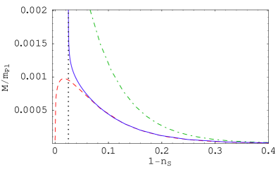
Then, one can take the following route. If one chooses a value for the scale $\mu$, then one can calculate $\varphi_{\mathrm{end}}$ with Eq. (48), $\varphi_{*}$ with Eq. (49) and, finally, the spectral index with the previous formula. Hence, instead of working with $\mu$, one can express everything in terms of $n_{{}_{\rm S}}$. Finally, using Eq. (43), one can determine the scale $M$ in terms of $\varphi_{*}$ and $\mu$ or, equivalently, in terms of the spectral index. In other words, we end up with an exact relation $M(n_{{}_{\rm S}})$. It is represented in Fig. 1 (solid blue line). As one can notice on this figure, the curve blows up at $n_{{}_{\rm S}}=1-6/(1+4N_{*})$. Let us try to understand this behavior in more details. If we expand the expression giving the spectral index in terms of the parameter $m_{{}_{\mathrm{Pl}}}/\mu$, one obtains $n_{{}_{\rm S}}=1-6/(1+4N_{*})+m_{{}_{\mathrm{Pl}}}/[\mu(1+4N_{*})^{2}\sqrt{\pi}]+{\cal O}\left(m_{{}_{\mathrm{Pl}}}/\mu\right)$ from which we can obtain an expression of $m_{{}_{\mathrm{Pl}}}/\mu$ in terms of $n_{{}_{\rm S}}$. In the same manner, one can expand $M$ and the result reads $\left(M/m_{{}_{\mathrm{Pl}}}\right)^{4}=45\pi^{2}/[(1+4N_{*})^{3/2}(m_{{}_{\mathrm{Pl}}}/\mu)]\left(Q_{\rm rms-PS}/T\right)^{2}+{\cal O}[(m_{{}_{\mathrm{Pl}}}/\mu)^{3}]$. Putting these two formulas together, one finally gets that

$$\left(\frac{M}{m_{{}_{\mathrm{Pl}}}}\right)^{4}\simeq \frac{45\pi^{3/2}}{(1+4N_{*})^{7/2}}\left(\frac{Q_{\rm rms-PS}}{T}\right)^{2}$$

$$\times\!\left(1-n_{{}_{\rm S}}-\frac{6}{1+4N_{*}}\right)^{\!-1}$$ (51)

up to terms of order $\mathcal{O}\left[(m_{{}_{\mathrm{Pl}}}/\mu)^{3}\right]$, and we now understand the presence of the singularity. Although exact for potentials of the form (34) (with $a=1$ and $b=-1$) , the behavior of $M$ is this regime is not realistic for the following reason: on general grounds, it is clear that it is necessary to consider additional terms in the potential (34) because, otherwise, $\varphi=\mu$ is not a minimum. If, during slow-roll inflation $\varphi\ll\mu$, then these terms are not important for the calculation of the perturbations. But, if $\mu\gg m_{{}_{\mathrm{Pl}}}$, then one has that $\phi_{\rm end}\sim\mu$ and we expect the extra terms to play a role even during slow-roll inflation. In this regime, the shape of the potential that we used in order to obtain that $M$ has a singularity is therefore not realistic. Moreover, it has been shown in Ref. [27] that the presence of these extra terms can strongly modify the energy scale of inflation.

Let us now try to understand the behavior of the curve far from the singularity. This can be analyzed in the regime where $\phi_{*}/\mu\ll 1$. In this situation, Eq. (50) tells us that

$$1-n_{{}_{\rm S}}\simeq\frac{m_{{}_{\mathrm{Pl}}}^{2}}{2\pi\mu^{2}}\,.$$ (52)

Moreover, since the Lambert function is small for small values of its argument, this also implies from Eq. (49) that [where we use $W_{0}(x)\simeq x$]

$$\left(\frac{\phi_{*}}{\mu}\right)^{\!2}\simeq\left(\frac{\phi_{\mathrm{end}}}{\mu}\right)^{\!2}\exp\!\left[-\left(\frac{\phi_{\mathrm{end}}}{\mu}\right)^{\!2}-\frac{N_{*}}{2\pi}\frac{m_{{}_{\mathrm{Pl}}}^{2}}{\mu^{2}}\right]\,.$$ (53)

The previous derivation is consistent as long as the term proportional to $N_{*}$ in the argument of the exponential in (53) is large rendering the argument of the Lambert function small. This implies that $N_{*}m_{{}_{\mathrm{Pl}}}^{2}/2\pi\mu^{2}\gtrsim 1$ and provides the consistency constraint $N_{*}(1-n_{{}_{\rm S}})\gtrsim 1$. This means that, in order for our approximation to hold, $n_{{}_{\rm S}}$ cannot be too close to $1$ which is fine since this is precisely the regime that we are interested in [as we are trying to approximate $M(n_{{}_{\rm S}})$ far from the singularity]. Another way to see the same thing is to remark that, if $n_{{}_{\rm S}}$ were too close to $1$, then, from Eq. (52), it would follow that $\mu\gg m_{{}_{\mathrm{Pl}}}$, in contradiction with the hypothesis that $\phi_{*}$ is exponentially damped, see Eq. (53).

Figure 1: Characteristic mass scale $M$ obtained from the CMB normalization as a function of the spectral index for the new inflationary scenario. The exact, numerically calculated, curve (solid blue line) blows up at $1-n_{{}_{\rm S}}=6/(1+4N_{*})$ while the approximated one (red dashed line) vanishes at the origin. A different approximation, usually found in the literature (see for instance Refs. [28, 29]), is also shown for comparison (green dotted-dashed line). The difference between these two lines is approximatively a factor of $2$ in $M$ and is significant since this leads to a factor of $16$ in the normalization factor $M^{4}$ of the potential and, thus, in the variance and the mean value of the fluctuations.

One the other hand, as is apparent from Fig. 1, we are not interested either in large values of $1-n_{{}_{\rm S}}$ which are, anyway, observationally excluded. Therefore, a Taylor expansion in this quantity is still valid in our case. In particular, using Eq. (52), one can express $\varphi_{\rm end}$, hence $\varphi_{*}$ and $\epsilon_{*}$, in terms of $1-n_{{}_{\rm S}}$ only. Finally, since $V_{*}\simeq M^{4}$, expanding everything in $1-n_{{}_{\rm S}}$, we can write Eq. (43) as

$$\left(\frac{M}{m_{{}_{\mathrm{Pl}}}}\right)^{\!4}\simeq\frac{45}{4}\frac{Q_{\mathrm{rms-PS}}^{\;2}}{T^{2}}(1-n_{{}_{\rm S}})\mathrm{e}^{-1-N_{*}(1-n_{{}_{\rm S}})}\,,$$ (54)

and we recover exactly the correct damping behavior observed in Fig. 1 (red dashed line).

Usually in the literature [28, 29], in the regime $\mu/m_{{}_{\mathrm{Pl}}}\ll 1$, one expands Eq. (48) to arrive at the expression $(\varphi_{\rm end}/\mu)\sim 2\sqrt{\pi}\mu/m_{{}_{\mathrm{Pl}}}$. Then, following the same steps as before, we end up with

$$\left(\frac{M}{m_{{}_{\mathrm{Pl}}}}\right)^{\!4}\simeq\frac{45}{2}\frac{Q_{\mathrm{rms-PS}}^{\;2}}{T^{2}}\mathrm{e}^{-N_{*}(1-n_{{}_{\rm S}})}\,,$$ (55)

This expression has to be compared with Eq. (54). The corresponding curve is represented in Fig. 1 (green dashed-dotted line). For $n_{{}_{\rm S}}-1$ not too close to zero, the two predictions are in good agreement.

Based on the above considerations, we arbitrarily choose to work with $n_{{}_{\rm S}}\simeq 0.93$ (compatible with the WMAP data) for which it follows that $\mu\sim 1.5m_{{}_{\mathrm{Pl}}}$. In this case, Fig. 1 indicates that

$$\left(\frac{M}{m_{{}_{\mathrm{Pl}}}}\right)^{4}\sim 10^{-12}\,.$$ (56)

This value corresponds to a regime which is compatible with the various approximations discussed above. We will adopt these values when plotting the quantum effects that we calculate in the following.

IV.4 Hybrid inflation

This case is slightly different since hybrid inflation is in fact a two-fields model with the potential [20]

$$V\left(\varphi,\psi\right)=\frac{1}{2}m^{2}\varphi^{2}+\frac{\lambda^{\prime}}{4}\left(\psi^{2}-\Delta^{2}\right)^{2}+\frac{\lambda}{2}\varphi^{2}\psi^{2}\,,$$ (57)

where $\varphi$ is the inflaton and $\psi$ the waterfall field. $\lambda^{\prime}$ and $\lambda$ are two coupling constants. The advantage of hybrid inflation is that inflation can be realized even if these coupling constants are of order one. The inflationary valley is given by $\psi=0$ and, in this case, the potential reduces to a potential similar to the one given in Eq. (34) with $a=1$ and $b=1$, provided we have

$$M=\frac{\lambda^{\prime}{}^{1/4}\Delta}{\sqrt{2}}\,,\quad\mu=\sqrt{\frac{\lambda^{\prime}}{2}}\frac{\Delta^{2}}{m}\,.$$ (58)

In the hybrid scenario there are a priori two mechanisms for ending inflation. Either inflation stops by instability when the inflaton reaches a value

$$\phi_{\rm cri}=\frac{\lambda^{\prime}}{\lambda}\Delta\,,$$ (59)

where the mass in the direction perpendicular to the inflationary valley becomes negative or the slow-roll conditions are violated which happen for

$$\frac{\phi_{\epsilon}}{m_{{}_{\mathrm{Pl}}}}=\sqrt{\frac{1}{8\pi}\left(1-\frac{8\pi\mu^{2}}{m_{{}_{\mathrm{Pl}}}^{2}}+\sqrt{1-\frac{16\pi\mu^{2}}{m_{{}_{\mathrm{Pl}}}^{2}}}\right)}\,.$$ (60)

Let us notice that $\phi_{\epsilon}$ does not exist if $\mu>m_{{}_{\mathrm{Pl}}}/(4\sqrt{\pi})$. Therefore, the final value of the inflaton, $\phi_{\mathrm{end}}$, is the maximum of $\phi_{\rm cri}$ and $\phi_{\epsilon}$. To decide which mechanism is realized in practice requires the knowledge of the parameters of the model. Of course, the parameters of the models must satisfy the CMB normalization [20]. The value of the field at horizon exit is given by an equation very similar to Eq. (49), namely

$$\frac{\phi_{*}}{\mu}=\sqrt{W_{0}\!\left\{\!\left(\!\frac{\phi_{\mathrm{end}}}{\mu}\!\right)^{\!2}\!\exp\!\left[\frac{\phi_{\mathrm{end}}^{2}+(N_{*}/2\pi)m_{{}_{\mathrm{Pl}}}^{2}}{\mu^{2}}\right]\!\right\}}\,.$$ (61)

Then, one can repeat the algorithm described in the previous subsection to implement the CMB normalization. Here, we assume that the coupling constants are $\lambda=\lambda^{\prime}=1$ and use the following values

$$\Delta=10^{-4}m_{{}_{\mathrm{Pl}}}\,,\quad m\simeq 0.7\times 10^{-8}m_{{}_{\mathrm{Pl}}}\,.$$ (62)

This implies $\mu\simeq 1.01m_{{}_{\mathrm{Pl}}}$ and $n_{{}_{\rm S}}\simeq 1.08$, i.e. a blue spectrum as expected for hybrid inflation. Let us remark that in the above case, inflation ends by instability and is vacuum dominated. This is the regime of interest for us because it would be pointless to calculate the quantum effects in the regime where the field dominates since this case reduces to the case of chaotic inflation.

IV.5 Running-mass Inflation

Running mass inflation can be realized in four different ways [21] that we now very briefly describe. In the following, we refer to these four different models as RM1 to RM4. From the expression of the potential (35), it is easy to see that $\varphi_{0}$ is an extremum of $V(\varphi)$. This is a maximum if $c>0$ and a minimum if $c<0$. According to the classification of Ref. [21], “model 1” (RM1) corresponds to the case where $c>0$ and $\varphi_{\mathrm{cl}}<\varphi_{0}$. In this case, $\varphi_{\mathrm{cl}}$ decreases during inflation. “Model 2” (RM2) also corresponds to $c>0$ but, now, with $\varphi_{\mathrm{cl}}>\varphi_{0}$ and $\varphi_{\mathrm{cl}}$ increases during inflation. “Model 3” (RM3) refers to the situation where $c<0$, for which $\varphi_{0}$ is a minimum, and $\varphi_{\mathrm{cl}}<\varphi_{0}$ all the time. In this case, $\varphi_{\mathrm{cl}}$ increases during inflation. Finally, “model 4” (RM4) has $c<0$ and $\varphi_{\mathrm{cl}}>\varphi_{0}$ decreases during inflation.

The values of the free parameters $c$ and $\varphi_{0}$ are constrained by the CMB measurements. In Ref. [21], these constraints have been studied for the four models evoked above in the parameter space $(c,\sigma)$, where $\sigma$ is defined by $\sigma=-c\ln\left(\varphi_{\rm end}/\varphi_{0}\right)$, $\varphi_{\rm end}$ being the value at which inflation stops. Using $\sigma$ allows us to express the spectral index and the running of the spectral index as

$$n_{{}_{\rm S}}-1\simeq-2c+2\sigma\mathrm{e}^{-cN_{*}}=-2c+\frac{1}{c}\frac{\mathrm{d}n_{{}_{\rm S}}}{\mathrm{d}\ln k}\,,$$ (63)

where $N_{*}$ has already been defined before.

Let us now study how inflation ends in those models. A priori, the end of inflation is found from the condition $\epsilon=1$. However, it is easy to see that this cannot be achieved for model 3 [for $V(\varphi_{0})\neq 0$] and model 4. In this case, another mechanism must be advocated, presumably of the hybrid type. For simplicity, in the following, we focus on models 1 and 2 only. In the case of model $1$, one can also show that the condition $\epsilon=1$ cannot be satisfied because $\epsilon\rightarrow 0$ when $\varphi\rightarrow 0$ and is bounded by $c^{2}\varphi_{0}^{2}/(16\pi eM_{{}_{\rm Pl}}^{2})\ll 1$ in the interval $[0,\varphi_{0}]$. However, the slow-roll parameter $\eta\equiv M_{{}_{\rm Pl}}^{2}V^{\prime\prime}/V$ (this slow-roll parameters differs from $\epsilon_{2}$ introduced above) increases when $\varphi\rightarrow 0$ and inflation stops when $\eta=1$. In the case of model 2, the condition $\epsilon=1$ is a priori possible but we will see that, in practice, the condition $\eta=1$ occurs earlier and, therefore, controls the end of inflation as for model 1.

As an illustration of model 1, we work with the values $c=0.06$ and $\varphi_{0}/M_{{}_{\rm Pl}}=10^{-6}$. In this case, the end of inflation occurs at $\varphi_{\rm end}/M_{{}_{\rm Pl}}\sim 2\times 10^{-14}$. The parameter $\sigma$ is given by $\sigma\sim 1.064$. One can check in Fig. 3 of Ref. [21] (left panel) that these values are compatible with the CMB constraints and, moreover, that they correspond to a situation where the Planck satellite will measure the running of the spectral index.

For model 2, the situation is slightly more complicated. If we use the same parameters $c$ and $\varphi_{0}$, then inflation ends at $\varphi_{\rm end}/M_{{}_{\rm Pl}}\sim 0.6$ which is fine since this value is smaller than one. However, this leads to $\sigma\sim-0.79$ which, according to Fig. 4 (left panel) of Ref. [21] is not acceptable. Clearly, a way to cure the previous problem is to increase the value of $\varphi_{0}$. Therefore, for instance, we could try $\varphi_{0}/M_{{}_{\rm Pl}}=0.1$ and $c=0.06$. In this case $\varphi_{\rm end}/M_{{}_{\rm Pl}}\sim 2.95$ and $\sigma\sim-0.2$. The values of $c$ and $\sigma$ are now compatible with the CMB constraints but, of course, the value of $\varphi_{\rm end}>M_{{}_{\rm Pl}}$ is problematic. For instance, the simple expression of the number of e-folds given by Eq. (41) would not be valid in this case because we have assumed $\varphi_{\mathrm{cl}}/M_{{}_{\rm Pl}}\ll 1$. Moreover, we should also include higher orders terms in the potential. For these reasons, and since we only want to illustrate how quantum effects behave in the running mass scenario with simple formulas, we will continue to assume that $c=0.06$ and $\varphi_{0}/M_{{}_{\rm Pl}}=10^{-6}$ even for model 2.

Finally, once $c$ and $\varphi_{0}$ have been chosen, the COBE normalization fixes the scale $M$ through the relation

$$\frac{M^{4}}{m_{{}_{\mathrm{Pl}}}^{4}}=\frac{45}{4}\frac{Q_{\mathrm{rms-PS}}^{2}}{T^{2}}\frac{\sigma^{2}\varphi_{0}^{2}}{M_{{}_{\rm Pl}}^{2}}\exp\!\left(\!-\frac{\sigma}{c}\mathrm{e}^{-cN_{*}}\!-2cN_{*}\!\right).$$ (64)

In the case of model $1$ this gives $M\sim 6.4\times 10^{-7}m_{{}_{\mathrm{Pl}}}$ while for model $2$ we have $M\sim 1.2\times 10^{-6}m_{{}_{\mathrm{Pl}}}$, where in both cases we have used $N_{*}=50$.

Having chosen the parameters, one must also specify the initial conditions. The total number of e-folds is given by

$$N_{{}_{\rm T}}=\frac{1}{c}\ln\left[\left(\ln\frac{\varphi_{\mathrm{in}}}{\varphi_{0}}\right)^{-1}\ln\frac{\varphi_{\rm end}}{\varphi_{0}}\right]\,.$$ (65)

Regardless of the sign of $c$, one can check that $N_{{}_{\rm T}}>0$. For model $1$, one takes $\varphi_{\mathrm{in}}=\left(1-10^{-5}\right)\varphi_{0}$ which gives $N_{{}_{\rm T}}\sim 240$, while for model 2 one chooses $\varphi_{\mathrm{in}}=\left(1+10^{-3}\right)\varphi_{0}$ which implies that $N_{{}_{\rm T}}\sim 165$.

V Results and Discussion

Having fixed the values of the parameters for the four models under consideration, we can now compute the quantum effects. Let us first apply our formalism to the potential (34) and study the behavior of the fluctuations in the different inflationary scenarios. In this case, Eq. (13) can be integrated exactly and straightforward calculations lead to

$$\frac{\left\langle\delta\varphi_{1}^{2}\right\rangle}{\mu^{2}}=\frac{4b}{3n}\frac{M^{4}}{m_{{}_{\mathrm{Pl}}}^{4}}\,\frac{I_{n}}{a+b(\varphi_{\mathrm{cl}}/\mu)^{n}}\left(\frac{\varphi_{\mathrm{cl}}}{\mu}\right)^{\!2(n-1)}\,,$$ (66)

with

$$I_{n} \equiv 4\!\int^{\varphi_{\mathrm{in}}/\mu}_{\varphi_{\mathrm{cl}}/\mu}\kern-10.00002pt\mathrm{d}x\,x^{3(1-n)}\left(a+bx^{n}\right)^{3}$$ (67)

$$=P_{n}\!\left(\frac{\varphi_{\mathrm{in}}}{\mu}\right)-P_{n}\!\left(\frac{\varphi_{\mathrm{cl}}}{\mu}\right)\,,$$ (68)

the function $P_{n}$ being given by

$$P_{n}(x)=x^{4}\bigg{(}b+\frac{4a\,x^{-3n}}{4-3n}-\frac{6ab\,x^{-2n}}{n-2}-\frac{12a\,x^{-n}}{n-4}\bigg{)}\,.$$ (69)

This expression is valid as long as $n\neq 2,4$ or $4/3$. These three particular cases must be treated separately and the corresponding function $P$ reads

$$P_{2}(x) =-2\frac{a}{x^{2}}+6ax^{2}+bx^{4}+12ab\ln x\,,$$ (70)

$$P_{4}(x) =-\frac{a}{2x^{8}}-3\frac{ab}{x^{4}}+bx^{4}+12a\ln x\,,$$ (71)

$$P_{4/3}(x) =9abx^{4/3}+\frac{9}{2}ax^{8/3}+bx^{4}+4a\ln x\,.$$ (72)

It is worth noticing that setting $a=0$ and $b=1$ we correctly recover the result obtained for a simple power law potential $V(\varphi)\propto\varphi^{n}$, namely

$$\frac{\left\langle\delta\varphi_{1}^{2}\right\rangle}{\mu^{2}}=\frac{4}{3n}\frac{M^{4}}{m_{{}_{\mathrm{Pl}}}^{4}}\left(\frac{\varphi_{\mathrm{cl}}}{\mu}\right)^{\!n-2}\left[\left(\frac{\varphi_{\mathrm{in}}}{\mu}\right)^{\!4}-\left(\frac{\varphi_{\mathrm{cl}}}{\mu}\right)^{\!4}\right].$$ (73)

This result was also derived in Ref. [13].

The next step consists in calculating the correction to the mean value. Using Eq. (15), this is immediately done once the variance is known and the result is

$$\frac{\left\langle\delta\varphi_{2}\right\rangle}{\mu}=Q_{n}\!\left(\frac{\varphi_{\mathrm{cl}}}{\mu}\right)\frac{\left\langle\delta\varphi_{1}^{2}\right\rangle}{\mu^{2}}+\frac{4b}{3n}\frac{M^{4}}{m_{{}_{\mathrm{Pl}}}^{4}}$$

$$\times\frac{(\varphi_{\mathrm{cl}}/\mu)^{n-1}}{\sqrt{a+b(\varphi_{\mathrm{cl}}/\mu)^{n}}}\!\left[R_{n}\!\left(\frac{\varphi_{\mathrm{in}}}{\mu}\right)-R_{n}\!\left(\frac{\varphi_{\mathrm{cl}}}{\mu}\right)\right],$$ (74)

where the two functions $Q_{n}$ and $R_{n}$ are defined by the following expressions

$$Q_{n}(x)\equiv\frac{2a(n-1)+b(n-2)x^{n}}{4x(a+bx^{n})}\,,$$ (75)

and

$$R_{n}(x)\equiv x^{2(1-n)}(a+bx^{n})^{5/2}\,.$$ (76)

Let us notice that, for $a=0$, these functions are simple power-laws and that, in this case, we recover the formulas found in Ref. [13] for generic monomial potentials.

The last step consists in computing the volume effects. For this purpose, we have to compute the integral in Eq. (33) for the potential (34). This leads to

$$\frac{\left\langle\varphi\right\rangle_{\rm v}-\left\langle\varphi\right\rangle}{\mu}=\frac{32\pi}{n^{2}}\frac{M^{4}\mu^{2}}{m_{{}_{\mathrm{Pl}}}^{6}}\left(\frac{\varphi_{\mathrm{cl}}}{\mu}\right)^{\!n-1}\left\{\frac{4}{\sqrt{a+b(\varphi_{\mathrm{cl}}/\mu)^{n}}}\left[S_{n}\!\left(\frac{\varphi_{\mathrm{in}}}{\mu}\right)-S_{n}\!\left(\frac{\varphi_{\mathrm{cl}}}{\mu}\right)\right]-P_{n}\!\left(\frac{\varphi_{\mathrm{in}}}{\mu}\right)+P_{n}\!\left(\frac{\varphi_{\mathrm{cl}}}{\mu}\right)\right\},$$ (77)

where $S_{n}$ is the function defined by the expression

$$S_{n}(x) =\int\mathrm{d}x\frac{(a+bx^{n})^{7/2}}{x^{3(n-1)}}$$ (78)

$$=a^{7/2}\frac{x^{4-3n}}{4-3n}\,{}_{2}F_{1}\!\!\left(\frac{4-3n}{n},-\frac{7}{2};\frac{4-2n}{n};-\frac{b}{a}x^{n}\right)\!,$$

for $a\neq 0$. In this expression ${}_{2}F_{1}(a,b;c;x)$ is the hypergeometric function taking real values for values of the argument $x$ less than one [24]. This is indeed the case since, for $b=1$, the argument is negative and for $b=-1$ we always have $(\varphi_{\mathrm{cl}}/\mu)^{n}<1$. If $a=0$ (in the large field models case), then the argument is ill-defined. However, using the relation for the hypergeometric function of argument $1/x$ [24] (that can be safely applied since, in this case, we have $b=1$) we obtain a well-defined expression that yields

$$S_{n}(x)=2\,\frac{x^{4+n/2}}{8+n}\,,$$ (79)

up to an unimportant additive constant.

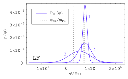
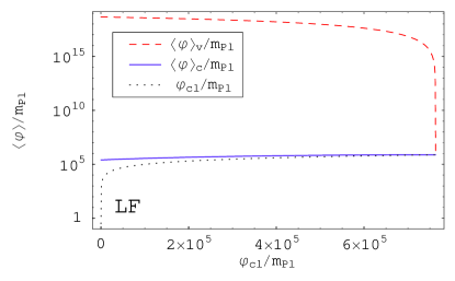
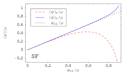
Once the variance and the mean value are known, calculating the probability distribution of the field is straightforward, see Eq. (25). Results for large field and small field models are shown in Fig. 2. For LF, we take an initial condition $\varphi_{\mathrm{in}}$ such that the potential energy is close to the Planck scale $m_{{}_{\mathrm{Pl}}}^{4}$. In this case, $P_{\mathrm{c}}$ (or rather its maximum $\left\langle\varphi\right\rangle_{\mathrm{c}}$) slowly rolls down the potential while remaining “behind” the classical solution. At the same time and very quickly after the initial time, the variance significantly increases, i.e. $P_{\mathrm{c}}$ strongly spreads, and, as a consequence, the tail of $P_{\mathrm{c}}$ penetrates into the region where $\varphi<0$. On the contrary, $P_{\mathrm{v}}$, while also spreading a lot, immediately inverts its motion, starts rolling up the potential and penetrates into the trans-Planckian regime where $V\gg m_{{}_{\mathrm{Pl}}}^{4}$. These behaviors confirm the importance of quantum fluctuations in the LF models but this also rises the question of the reliability of the solutions obtained before. Indeed, in the case of $P_{\mathrm{c}}$, for $\varphi<\varphi_{\mathrm{end}}$ (a few $m_{{}_{\mathrm{Pl}}}$’s) the Hubble crossing of the modes stops and the noise no longer exists. Moreover, the slow-roll approximation that we have explicitly used in our derivation of the Langevin equation is no longer valid. With regards to $P_{\mathrm{v}}$, in the regime where $V>m_{{}_{\mathrm{Pl}}}^{4}$, the whole framework of quantum field theory itself breaks down. These features are also very sensitive to the initial conditions. For instance, if we have initially $V(\varphi_{\mathrm{in}})<m_{{}_{\mathrm{Pl}}}^{4}/10$, then the stochastic deviations from the classical trajectory are already dramatically reduced.

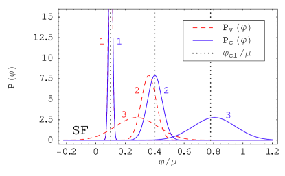
In the case of SF models similar conclusions hold. If $\varphi_{\mathrm{in}}$ is very small (close the maximum of the potential), then $P_{\mathrm{c}}$ significantly spreads around its mean value while rolling down the potential. The only difference is that, now, the peak of the distribution stays ahead of $\varphi_{\mathrm{cl}}$. As before, the tail of the single-point distribution goes to the region where the slow-roll approximation breaks down, $\varphi>\varphi_{\mathrm{end}}$ and $\varphi>\mu$. In this case, the previous considerations on the reliability of the solution still apply. Let us now study the behavior of $P_{\mathrm{v}}$. As can be seen in Fig. 2, at the beginning of inflation, the behaviors of $P_{\mathrm{c}}$ and $P_{\mathrm{v}}$ are similar but, after a few e-foldings, $P_{\mathrm{v}}$ reverses its motion and starts moving back towards the maximum located at $\varphi=0$. After enough time, most of $P_{\mathrm{v}}$ is on the other side of the potential. Diffusion is less crucial than in the LF models because the energy scales involved are smaller but, nonetheless, we see that such effects are very important. On the other hand, the behavior of $P_{\mathrm{v}}$ is less problematic since the Langevin equation is fully trustable even if the field is negative (provided, of course, it is still small in comparison to $\mu$). The only danger comes from a possible breakdown of the perturbative expansion as the field goes to a region where the stochastic mean value is very far from its classical counterpart. In this case, the quantum effects should in fact be computed as perturbations of a classical solution living in the region $\varphi<0$. Then, the volume effects will act the same way as before, that is to say they will push the corresponding distribution back to the origin, towards the region $\varphi>0$. Therefore, it seems reasonable to postulate that a situation of dynamical equilibrium could set up with a stationary solution for $P_{\mathrm{v}}$ concentrated around $\varphi=0$.

Finally, let us notice that, as before, the stochastic behavior of the field is strongly dependent on the initial conditions. If $\varphi$ is far from the maximum, then the drift due to the classical term dominates on the noise-induced diffusion, the effect of which is therefore no longer important. The dependence on the initial conditions can be also be checked with the help of Eq. (66) in the limit $\varphi_{\mathrm{cl}}\ll\mu$. In this regime we have $P_{2}(x)\simeq-2/x^{2}$ and, since $\varphi_{\mathrm{in}}<\varphi_{\mathrm{cl}}$, the relative amplitude of the fluctuations can be written as

$$\frac{\sqrt{\left\langle\delta\varphi_{1}^{2}\right\rangle}}{\varphi_{\mathrm{cl}}}\lesssim\sqrt{\frac{4}{3}}\left(\frac{M}{m_{{}_{\mathrm{Pl}}}}\right)^{\!2}\frac{\mu}{\varphi_{\mathrm{in}}}\sim 10^{-1}\,,$$ (80)

for $M\sim 10^{-3}m_{{}_{\mathrm{Pl}}}$ and $\varphi_{\mathrm{in}}\sim 10^{-5}\mu$. This shows that, in this case, the stochastic fluctuations can represent up to 10% of the field value (and they increase in the subsequent evolution since, in new inflation, different classical solutions diverge). However, taking another initial condition, for instance $\varphi_{\mathrm{in}}/\mu\simeq 10^{-3}$, would reduce the fluctuations to only 0.1% of the classical field. Therefore, we see that there is indeed a strong dependence on the initial conditions.

Let us now consider hybrid inflation in the vacuum dominated regime. In this case, the corresponding distributions are so peaked that they cannot be distinguished from a Dirac distribution. This is the reason why we have chosen not to include any figure for the hybrid case. The reason for this behavior can be easily understood if we come back to Eq. (66). In this case, $\varphi_{\mathrm{in}}>\varphi_{\mathrm{cl}}>\varphi_{\mathrm{cri}}$ and, therefore, one has

$$\frac{\sqrt{\left\langle\delta\varphi_{1}^{2}\right\rangle}}{\varphi_{\mathrm{cl}}}\sim\sqrt{\frac{4}{3}}\left(\frac{M}{m_{{}_{\mathrm{Pl}}}}\right)^{\!2}\frac{\mu}{\varphi_{\mathrm{cl}}}\,,$$ (81)

the upper limit of the above expression being obtained when evaluated for $\varphi=\varphi_{\rm cri}$. Using Eqs. (58) and (59), one arrives at

$$\frac{\sqrt{\left\langle\delta\varphi_{1}^{2}\right\rangle}}{\varphi_{\mathrm{cl}}}\lesssim\frac{\Delta^{3}}{mm_{{}_{\mathrm{Pl}}}^{2}}\sim 10^{-4}\,,$$ (82)

for the values of $\Delta$ and $m$ chosen before. Therefore, in hybrid vacuum dominated models, the fluctuations are less than 0.1% of the classical field until the very end of inflation. In addition, if one uses Eq. (V) in the same limit, one sees that the two terms of that formula exactly cancels out and $\left\langle\delta\varphi_{2}\right\rangle\sim 0$. This means that, with a very good accuracy, the distributions are peaked over the classical value of the field. This explains the behavior of the distribution functions described before. Moreover, this conclusion is rather independent of the initial condition, provided that the latter does not violate the vacuum dominated regime.

Figure 2: Evolution of the single-point (solid blue line) and volume-weighted (dashed red line) probability distributions, $P_{\mathrm{c}}(\varphi)$ and $P_{\mathrm{v}}(\varphi)$, for the large field model $V\propto\varphi^{2}$ (LF) and the small field model $V\propto 1-(\varphi/\mu)^{2}$ (SF). The initial values are $\varphi_{\mathrm{in}}=7.6\times 10^{5}m_{{}_{\mathrm{Pl}}}$ (corresponding to $V_{\mathrm{in}}=m_{{}_{\mathrm{Pl}}}^{4}/2$) for LF and $\varphi_{\mathrm{in}}/\mu=10^{-5}$ for SF. The initial shape of the two probability density functions is always chosen to be $\delta(\varphi-\varphi_{\mathrm{in}})$. The vertical dotted black lines represent the location of the classical field. Three successive snapshots of the distributions (numbered $1$, $2$ and $3$) are shown on the left panels while the evolution of $\left\langle\varphi\right\rangle_{\mathrm{c}}$ and $\left\langle\varphi\right\rangle_{\mathrm{v}}$ is displayed on the right panels. The classical field $\varphi_{\mathrm{cl}}$ evolves from the right to the left in LF and from the left to the right in SF. In both cases, $P_{\mathrm{c}}(\varphi)$ rolls down the potential, spreads significantly around its mean value and penetrates into a classically forbidden region ($\varphi<0$ for LF and $\varphi>\mu$ for SF). The quantity $\left\langle\varphi\right\rangle_{\mathrm{c}}$ stays “behind” the classical value in LF but is “ahead” in SF. On the other hand, $P_{\mathrm{v}}(\varphi)$ (not shown in the LF left panel) reverses its motion and climbs towards the trans-Planckian region (in LF) or towards the maximum of the potential at $\varphi=0$ in SF.

Figure 3: Evolution of the single-point (solid blue line) and volume-weighted (dashed red line) probability distributions for the two different running mass inflation models RM1 and RM2. The initial probability density function is $\delta(\varphi-\varphi_{\mathrm{in}})$ for the two models. The initial values are chosen to be $\varphi_{\mathrm{in}}/\varphi_{0}=1-1.5\times 10^{-5}$ for RM1 ($\varphi<\varphi_{0}$, inflation proceeding from the right to the left) and $\varphi_{\mathrm{in}}/\varphi_{0}=1+10^{-3}$ for RM2 ($\varphi>\varphi_{0}$, inflation proceeding from the left to the right). The vertical lines (dotted black lines) represent the location of the classical field. On the two left panels, three snapshots of $P_{\mathrm{c}}(\varphi)$ and $P_{\mathrm{v}}(\varphi)$ (numbered from $1$ to $3$) are shown at three different times (respectively corresponding for RM1 to $\varphi/\varphi_{0}=0.9,0.5$ and $0.01$) together with the corresponding values of the classical field. In the right panels, the evolution of $\left\langle\varphi\right\rangle_{\mathrm{c}}$ and $\left\langle\varphi\right\rangle_{\mathrm{v}}$ is followed until the end of inflation. The physical interpretation of these results is discussed in the text.

Let us now investigate the quantum effects for the two different models of running mass inflation. The variance and the mean value can be calculated exactly since the corresponding integrals are feasible. This results in quite complicated formulas which are not especially illuminating. However, since the vacuum expectation value of the inflaton is always small with respect to the Planck mass, it is therefore a good approximation to replace $V^{\prime}/V$ by $V^{\prime}/M^{4}$ as we have already done before, see Ref. [21]. Then, the variance reads

$$\frac{\left\langle\delta\varphi_{1}^{2}\right\rangle}{M_{{}_{\mathrm{Pl}}}^{2}} = \frac{1}{12\pi^{2}c}\left(\frac{M}{M_{{}_{\mathrm{Pl}}}}\right)^{4}\left(\frac{\varphi_{\mathrm{cl}}}{\varphi_{0}}\right)^{2}\ln^{2}\left(\frac{\varphi_{\mathrm{cl}}}{\varphi_{0}}\right)\biggl{[}\frac{1}{2}\left(\frac{\varphi_{0}}{\varphi_{\mathrm{in}}}\right)^{2}\frac{1}{\ln^{2}\left(\varphi_{\mathrm{in}}/\varphi_{0}\right)}-\frac{1}{2}\left(\frac{\varphi_{0}}{\varphi_{\mathrm{cl}}}\right)^{2}\frac{1}{\ln^{2}\left(\varphi_{\mathrm{cl}}/\varphi_{0}\right)}$$ (83)

$$+\left(\frac{\varphi_{0}}{\varphi_{\mathrm{cl}}}\right)^{2}\frac{1}{\ln\left(\varphi_{\mathrm{cl}}/\varphi_{0}\right)}-\left(\frac{\varphi_{0}}{\varphi_{\mathrm{in}}}\right)^{2}\frac{1}{\ln\left(\varphi_{\mathrm{in}}/\varphi_{0}\right)}+2{\rm Ei}\left(-2\ln\frac{\varphi_{\mathrm{cl}}}{\varphi_{0}}\right)-2{\rm Ei}\left(-2\ln\frac{\varphi_{\mathrm{in}}}{\varphi_{0}}\right)\biggr{]}\,.$$

¿From this result, using Eq. (15), we deduce the expression of the mean value, namely

$$\frac{\left\langle\delta\varphi_{2}\right\rangle}{M_{{}_{\rm Pl}}} = \frac{1}{2}\left[\frac{1+\ln\left(\varphi_{\mathrm{cl}}/\varphi_{0}\right)}{\left(\varphi_{\mathrm{cl}}/M_{{}_{\rm Pl}}\right)\ln\left(\varphi_{\mathrm{cl}}/\varphi_{0}\right)}+\frac{c}{2}\frac{\varphi}{M_{{}_{\rm Pl}}}\ln\frac{\varphi_{\mathrm{cl}}}{\varphi_{0}}\right]\frac{\left\langle\delta\varphi_{1}^{2}\right\rangle}{M_{{}_{\rm Pl}}^{2}}+\frac{1}{48\pi^{2}c}\left(\frac{M}{M_{{}_{\rm Pl}}}\right)^{4}\frac{\varphi_{\mathrm{cl}}}{M_{{}_{\rm Pl}}}\ln\left(\frac{\varphi_{\mathrm{cl}}}{\varphi_{0}}\right)$$ (84)

$$\times\left[\left(\frac{M_{{}_{\rm Pl}}}{\varphi_{\mathrm{cl}}}\right)^{2}\frac{1}{\ln^{2}\left(\varphi_{\mathrm{cl}}/\varphi_{0}\right)}-\left(\frac{M_{{}_{\rm Pl}}}{\varphi_{\mathrm{in}}}\right)^{2}\frac{1}{\ln^{2}\left(\varphi_{\mathrm{in}}/\varphi_{0}\right)}\right]\,.$$

Finally, let us compute the volume effects given by Eq. (33). Following the approximation already used above, one could take a factor $H$ out of the integral. Then, the remaining integral, the kernel of which is now $(H/H^{\prime})^{3}$, can be performed explicitly. However, in this case, the result exactly cancel the second term in Eq. (33) and we would obtain $\left\langle\varphi\right\rangle_{\rm v}-\left\langle\varphi\right\rangle\simeq 0$. Let us notice that this is is not a specific feature of the running mass potential but a general consequence of the approximation used. Therefore, in order to compute the volume effects, one should evaluate the original integral. Unfortunately, an exact integration is not possible in this case. A possible solution is then to expand the integrand in powers of $c(\varphi_{0}/M_{{}_{\mathrm{Pl}}})^{2}$. At first order, this gives

$$3I^{T}J = -\frac{7M}{16\pi^{2}c}\frac{M^{3}}{M_{{}_{\rm Pl}}^{3}}\frac{\varphi_{\mathrm{cl}}}{M_{{}_{\rm Pl}}}\ln\frac{\varphi_{\mathrm{cl}}}{\varphi_{0}}\left[1-\frac{c}{2}\left(-\frac{1}{2}+\ln\frac{\varphi_{\mathrm{cl}}}{\varphi_{0}}\right)\frac{\varphi_{\mathrm{cl}}^{2}}{M_{{}_{\rm Pl}}^{2}}\right]^{-1/2}$$ (85)

$$\times\left[-\frac{1}{\ln(\varphi_{\mathrm{in}}/\varphi_{0})}+\frac{1}{\ln(\varphi_{\mathrm{cl}}/\varphi_{0})}+\frac{1}{4\ln^{2}(\varphi_{\mathrm{in}}/\varphi_{0})}-\frac{1}{4\ln^{2}(\varphi_{\mathrm{cl}}/\varphi_{0})}\right]\,.$$

Alternatively, a numerical integration of Eq. (33) can always be done and, in the following, we present results obtained with this method.

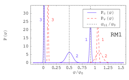
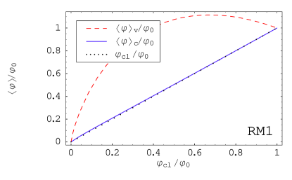
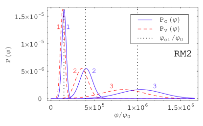
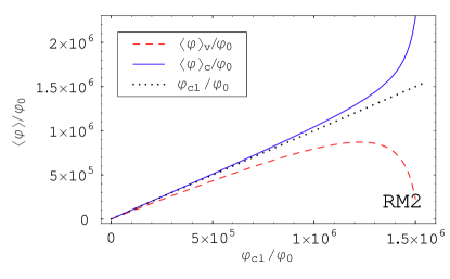
Results for RM1 and RM2 are displayed in Fig. 3. Let us start with the RM1 model. In this case, $P_{\mathrm{c}}(\varphi)$ follows very closely the classical solution, the peak of the distribution being slightly “behind” $\varphi_{\mathrm{cl}}$ (as for LF). Interestingly enough, if, at the beginning of inflation, the distribution $P_{\mathrm{c}}(\varphi)$ starts spreading around its mean value as it was the case for the LF and SF models then, after some e-foldings, the variance reaches a maximum and then starts decreasing, i.e. $P_{\mathrm{c}}(\varphi)$ becomes more and more peaked over the classical solution. This is a consequence of the fact that the classical dynamics (which dominates at late times) tends to attract different solutions contrarily to the SF case where they are instead pulled apart. The behavior of $P_{\mathrm{v}}(\varphi)$ is even more interesting. The volume weighted distribution moves backwards, beyond the maximum of the potential, into the region classically corresponding to RM2. Then, it reverses its motion and comes back into the region corresponding to RM1. This last behavior is probably not trustable because, as long as $P_{\mathrm{v}}(\varphi)$ penetrates the region RM2, the calculations performed before should be modified to take this situation into account. Let us also notice that this behavior is not exactly similar to the one observed for the SF model where the distribution goes to the region $\varphi<0$, see the discussion above. Indeed, in this last case, whatever the sign of the field, the model is the same, in particular the value of $M$ remains unchanged. On the contrary, RM1 and RM2 are really two different models with two different energy scales. Let us now study RM2. As for RM1, the peak of $P_{\mathrm{c}}(\varphi)$ follows the classical solution with the difference, however, that it is slightly ahead $\varphi_{\mathrm{cl}}$ (as for SF) and that the spreading of the distribution continuously increases. At the beginning of inflation, $P_{\mathrm{v}}(\varphi)$ also follows $\varphi_{\mathrm{cl}}$ but, then, it changes its motion and moves back towards the region corresponding to RM1.

One of our main conclusion concerning running mass inflation is that, if RM1 and RM2 are classically two different models, from a statistical point of view, it may then be impossible to distinguish between them. Indeed, regardless of which model we decide to start with, if the initial conditions are sufficiently close to $\varphi_{0}$, then there is a significant probability of diffusing on the other side of the potential. Moreover, when we start with RM1 (RM2), volume effects tends to push the evolution towards RM2 (RM1). Therefore, as it was the case for SF, it seems reasonable to postulate that the system will settle down at the boundary between the two models, a situation described by a stationary distribution concentrated around $\varphi_{0}$. Such a situation typically leads to the self-reproducing regime.

Finally, another important feature of the running mass potential is that quantum effects can strongly modify the classical evolution even if the energy scale involved is far below the Planck energy (this is also the case for new inflation). This reinforces the fact that the connection between the importance of the quantum effects on one hand and the fact that $V$ is close to the Planck energy on the other hand is very specific to the large field monomial potentials used in chaotic inflation. In fact, it is clear that quantum fluctuations are important whenever the classical contribution to the motion of the field is suppressed. In chaotic inflation, this happens close the Planck scale because of the large friction term but this also happens near the maximum of the potential (and far from the Planck scale) in new and running mass inflation models because of the smallness of $V^{\prime}(\varphi)$.

We end this section by a slightly different discussion. In Ref. [11], eternal inflation is studied using the Langevin equation for the model $V(\varphi)\propto\varphi^{4}$. The main argument presented for considering this simple model is that analytical progress may be made in this case. Using the method presented in our article, one can in fact consider a much larger variety of models and one is not restricted to the simple chaotic quartic model. In order to illustrate this claim we consider the calculation, presented in Ref. [11], of the value of the inflaton at which the self-reproducing behavior becomes possible, not only for the potential $\varphi^{4}$ but for the general case $\varphi^{n}$ (in fact, one could even reproduce this calculation for new inflation, running mass inflation and so on).

In Ref. [11], the main idea is to evaluate the mean value of the number of e-folds is given by

$$\left\langle N\right\rangle=\int_{0}^{T}\mathrm{d}t\left\langle H\right\rangle=-\frac{\kappa}{2}\int_{\varphi_{\mathrm{in}}}^{\varphi(T)}\mathrm{d}\psi\frac{\left\langle H\right\rangle}{H^{\prime}_{\mathrm{cl}}}\,.$$ (86)

This expression can easily be evaluated for any potential using our perturbative treatment. For large fields models, straightforward calculations lead to

$$\left\langle N\right\rangle=N_{{}_{\rm T}}^{\rm cl}\left[1+\frac{4(3n+4)M^{4}}{3n(n+2)m_{{}_{\mathrm{Pl}}}^{4}}\left(\frac{\varphi_{\mathrm{in}}}{m_{{}_{\mathrm{Pl}}}}\right)^{n}+\cdots\right]\,.$$ (87)

The breakdown of this expansion signals the beginning of the self-reproducing regime. Using the fact that $N_{{}_{\rm T}}^{\rm cl}\simeq 4\pi(\varphi_{\mathrm{in}}/m_{{}_{\mathrm{Pl}}})^{2}/n$, one easily sees that this happens when the initial value of the field is

$$\frac{\varphi_{\mathrm{in}}}{m_{{}_{\mathrm{Pl}}}}\sim\lambda_{n}^{-1/(n+2)}\,,$$ (88)

where the coupling constant $\lambda_{n}$ is defined such that $M^{4}/m_{{}_{\mathrm{Pl}}}^{n}=\lambda_{n}/m_{{}_{\mathrm{Pl}}}^{n-4}$. For $n=4$ one recovers the condition found in Ref. [11]. Our method allows us to obtain this condition for any potential and there is no need to assume a quartic potential to perform this calculation explicitly. Incidentally, the above condition was also found previously for instance in Ref. [7] [see Eq. (3.31)].

VI Conclusions

We now quickly summarize what are the new results obtained in this article. First, we have presented a perturbative method, used for the first time in Ref. [12], for solving the Langevin equation of stochastic inflation with, and this is crucial for the present article, the backreaction taken into account. We have compared this formalism with the other methods already known in the literature and have argued that it is more powerful because the approximation is made directly in the Langevin equation rather than in its solution. In particular, we were able to provide a general second order expression for the probability distribution of the field with or without the volume effects taken into account. Our expression only requires the calculation of one quadrature (two if the volume effects are considered) which, for most of the inflationary scenarios, can be performed explicitly. Second, we have applied this method to various models of inflation. This has allowed us to compute the quantum effects with backreaction for chaotic, new, hybrid and running mass inflation. To our knowledge, in the case of the last three models, this is the first time that such a calculation is done (the backreaction being taken into account). Third, we have discussed the impact of the stochastic effects on these inflationary scenarios. For instance, in the case of running mass inflation, it was shown that the quantum effects blur the distinction between the various running mass inflationary models and that the self-reproducing regime is likely to be important.

Finally, an important advantage of the method presented here is that its accuracy and domain of validity can be evaluated in details. This will be the subject of a forthcoming paper [15].

VII Acknowledgments

M. M. would like to thank the Università degli Studi di Milano and the Institut d’Astrophysique de Paris (IAP) where part of this work has been done. We would like to thank Patrick Peter for careful reading of the manuscript. It is a pleasure to thank André Grodemouge for useful comments.

The work of M. M. is supported by the National Science Foundation under Grant Nos. PHY-0071512 and PHY-0455649, and with grant support from the US Navy, Office of Naval Research, Grant Nos. N00014-03-1-0639 and N00014-04-1-0336, Quantum Optics Initiative.

Appendix A General Definitions

In this short Appendix, we give the precise definitions of the quantities that we have been using in order to establish the expression of the probability density function in Sec. III C. If we define a “two-step” function $\vartheta(t_{\mathrm{in}}<\tau<t)\equiv\vartheta(t-\tau)\vartheta(\tau-t_{\mathrm{in}})$ (whose value is 1 if the inequality is true and 0 otherwise), the expression of the “vector” $J$ is

$$J_{t,t_{\mathrm{in}}}(\tau)=\vartheta(t_{\mathrm{in}}<\tau<t)\frac{H^{\prime}_{\mathrm{cl}}(t)}{2\pi}\frac{H^{3/2}_{\mathrm{cl}}(\tau)}{H^{\prime}_{\mathrm{cl}}(\tau)}$$ (89)

while the “matrix”A can be written as

$$\mathbf{A}_{t,t_{\mathrm{in}}}(\sigma_{1},\sigma_{2})=\frac{H^{\prime}_{\mathrm{cl}}(t)}{4\pi}\left[3\vartheta(t_{\mathrm{in}}<\sigma_{1}<t)\sqrt{H_{\mathrm{cl}}(\sigma_{1})}J_{\sigma_{1},t_{\mathrm{in}}}(\sigma_{2})-\frac{m_{{}_{\mathrm{Pl}}}^{2}}{2}\!\int_{t_{\mathrm{in}}}^{t}\!\mathrm{d}\tau\frac{H^{\prime\prime\prime}_{\mathrm{cl}}(\tau)}{H^{\prime}_{\mathrm{cl}}(\tau)}J_{\tau,t_{\mathrm{in}}}(\sigma_{1})J_{\tau,t_{\mathrm{in}}}(\sigma_{2})\right].$$ (90)

Finally, we also provide the definitions of quantities that have been using in Sec. III D where the volume effects have been estimated. In particular, the “vector” $I$ can be expressed as

$$I_{t,t_{\mathrm{in}}}(\sigma)=3\!\int_{t_{\mathrm{in}}}^{t}\mathrm{d}\tau H^{\prime}_{\mathrm{cl}}(\tau)J_{\tau,t_{\mathrm{in}}}(\sigma)\,,$$ (91)

and the “matrix” ${\bf B}$ is defined by the following formula

$$\mathbf{B}_{t,t_{\mathrm{in}}}(\sigma_{1},\sigma_{2})=\int_{t_{\mathrm{in}}}^{t}\mathrm{d}\tau\left[H^{\prime}_{\mathrm{cl}}(\tau)\mathbf{A}_{\tau,t_{\mathrm{in}}}(\sigma_{1},\sigma_{2})+\frac{H^{\prime\prime}_{\mathrm{cl}}(\tau)}{2}J_{\tau,t_{\mathrm{in}}}(\sigma_{1})J_{\tau,t_{\mathrm{in}}}(\sigma_{2})\right]\,.$$ (92)

References

- [1] A. Vilenkin, Nucl. Phys. B226, 527 (1983); A. Vilenkin, Phys. Rev. D 27, 2848 (1983); A. S. Goncharov, A. D. Linde and V. F. Mukhanov, Int. J. Mod. Phys. A 2, 561 (1987); A. D. Linde, D. A. Linde and A. Mezhlumian, Phys. Rev. D 49, 1783 (1994).
- [2] A. A. Starobinsky, in Field Theory, Quantum Gravity and Strings, H. J De Vega, N. Sanchez Eds., 107 (1986).
- [3] S. J. Rey, Nucl. Phys. B 284, 706 (1987).
- [4] K. I. Nakao, Y. Nambu and M. Sasaki, Prog. Theor. Phys. 80, 1041 (1988).
- [5] H. E. Kandrup, Phys. Rev. D 39, 2245 (1989).
- [6] Y. Nambu and M. Sasaki, Phys. Lett. B 219, 240 (1989).
- [7] Y. Nambu, Prog. Theor. Phys. 81, 1037 (1989).
- [8] A. A. Starobinsky and J. Yokoyama, Phys. Rev. D 50, 6357 (1994).
- [9] H. M. Hodges, Phys. Rev. D 39, 3568 (1989).
- [10] I. Yi, E. T. Vishniac and S. Mineshige, Phys. Rev. D 43, 362 (1991).
- [11] S. Gratton and N. Turok, Phys. Rev. D 72, 043507 (2005), hep-th/0503063.
- [12] A. Gangui, F. Lucchin, S. Matarrese and S. Mollerach, Astrophys. J. 430, 447 (1994), astro-ph/9312033.
- [13] J. Martin and M. Musso, Phys. Rev. D 71, 063514 (2005), astro-ph/0410190.
- [14] S. Matarrese, A. Ortolan and F. Lucchin, Phys. Rev. D 40, 290 (1989).
- [15] J. Martin and M. Musso, in preparation.
- [16] S. Matarrese, L. Verde and R. Jimenez, Astrophys. J. 541, 10 (2000), astro-ph/0001366; S. Matarrese, M. Musso and A. Riotto, JCAP 0405, 008 (2004), hep-th/0311059.
- [17] J. Zinn-Justin, Intégrales de chemin en mécanique quantique : Introduction, CNRS-éditions, Paris (2003).
- [18] A. D. Linde, Phys. Lett. B 129, 177 (1983).
- [19] A. D. Linde, Phys. Lett. B 108, 389 (1982); 114, 431 (1982); 116, 335 (1982); 116, 340 (1982); A. Albrecht and P. J. Steinhardt, Phys. Rev. Lett. 48, 1220 (1982).
- [20] A. D. Linde, Phys. Lett. B 259, 38 (1991); E. J. Copeland et al, Phys. Rev. D 49, 6410 (1994), astro-ph/9401011.
- [21] L. Covi and D. H. Lyth, Phys. Rev. D 59, 063515 (1999), hep-ph/9809562.
- [22] L. Covi, D. H. Lyth and A. Melchiorri, Phys. Rev. D 67, 043507 (2003), hep-ph/0210395; L. Covi, D. H. Lyth, A. Melchiorri and C. J. Odman, Phys. Rev. D 70, 123521 (2004), hep-ph/0408129.
- [23] S. R. Valluri, D. J. Jeffrey and R. M. Corless, Can. J. Phys. 78, 823 (2000).
- [24] I. S. Gradshteyn and I. M. Ryshik, Table of Integrals, Series and Products, (Academic Press, New York, 1980); M. Abramowitz and I. A. Stegun, Handbook of Mathematical Functions, (Dover publications, New York, 1964); J. C. P. Miller, Tables of Weber Parabolic Cylinder Functions, (Her Majesty’s Stationery Office, 1955).
- [25] S. Leach and A. Liddle, Phys. Rev. D 68, 123508 (2003), astro-ph/0306305.
- [26] D. J. Schwarz, C. A. Terrero-Escalante and A. A. Garcia, Phys. Lett. B 517, 243 (2001), astro-ph/0202094.
- [27] G. German, G. Ross and S. Sarkar, Nucl. Phys. B 608, 423 (2001), hep-ph/0103243.
- [28] W. H. Kinney and K. T. Mahanthappa, Phys. Rev. D 53, 5455 (1996), hep-ph/9512241.
- [29] J. Martin, Braz. J. Phys. 34, 1307 (2004), astro-ph/0312492.