In Search of Lost Online Test-time Adaptation: A Survey

Abstract

This paper presents a comprehensive survey on online test-time adaptation (OTTA), a paradigm focused on adapting machine learning models to novel data distributions upon batch arrival. Despite the recent proliferation of OTTA methods, the field is mired in issues like ambiguous settings, antiquated backbones, and inconsistent hyperparameter tuning, obfuscating the real challenges and making reproducibility elusive. For clarity and a rigorous comparison, we classify OTTA techniques into three primary categories and subject them to benchmarks using the potent Vision Transformer (ViT) backbone to discover genuinely effective strategies. Our benchmarks span conventional corrupted datasets such as CIFAR-10$/$100-C and ImageNet-C and real-world shifts embodied in CIFAR-10.1 and CIFAR-10-Warehouse, encapsulating variations across search engines and synthesized data by diffusion models. To gauge efficiency in online scenarios, we introduce novel evaluation metrics, including GFLOPs, shedding light on the trade-offs between adaptation accuracy and computational overhead. Our findings diverge from existing literature, indicating: (1) transformers exhibit heightened resilience to diverse domain shifts, (2) the efficacy of many OTTA methods hinges on ample batch sizes, and (3) stability in optimization and resistance to perturbations are critical during adaptation, especially when the batch size is 1. Motivated by these insights, we pointed out promising directions for future research.

1 Introduction

Dataset shift (Quinonero-Candela et al, 2008) poses a notable challenge for machine learning. Models often experience significant performance drops when confronting test data characterized by conspicuous distribution differences from training. Such differences might come from changes in style and lighting conditions and various forms of corruption, making test data deviate from the data upon which these models were initially trained. To mitigate the performance degradation during inference, test-time adaptation (TTA) has emerged as a promising solution. TTA aims to rectify the dataset shift issue by adapting the model to novel distributions using unlabeled test data (Liang et al, 2023). Different from the traditional paradigm of domain adaptation (Ganin and Lempitsky, 2015; Wang and Deng, 2018), TTA does not require access to source data for distribution alignment. Commonly used strategies in TTA include unsupervised proxy objectives, spanning techniques such as pseudo-labeling Liang et al (2020), graph-based learning (Luo et al, 2023), and contrastive learning Chen et al (2022), applied on the test data through multiple training epochs to enhance model accuracy, such as autonomous vehicle detection (Hegde et al, 2021), pose estimation (Lee et al, 2023), video depth prediction (Liu et al, 2023a), frame interpolation (Choi et al, 2021), and medical diagnosis (Ma et al, 2022; Wang et al, 2022b; Saltori et al, 2022). Nevertheless, requiring access to the complete test set at every time step may not always align with practical use. In many applications, such as autonomous driving, adaptation is restricted to using only the current test batch processed in a streaming manner. Such operational restrictions make it untenable for TTA to require the full test set tenable.

In this study, our focus is on a specific line of TTA methods, i.e., online test-time adaptation (OTTA), which aims to accommodate real-time changes in the test data distribution. We provide a comprehensive overview of existing OTTA studies and evaluate the efficiency and effectiveness of these methods and their individual components. To facilitate a structured comprehension of the OTTA landscape, we categorize existing approaches into three groups: data-centric OTTA, model-based OTTA, and optimization-oriented OTTA.

• Data-based OTTA maximizes prediction consistency across diversified test data. Diversification strategies use auxiliary data, improved data augmentation methods, and diffusion techniques and create a saving queue for test data, etc.

• Model-based OTTA changes the original backbone, such as modifying specific layers or their mechanisms, adding supplementary branches, and incorporating prompts.

• Optimization-based OTTA focuses on various optimization methods. Examples are designing new loss functions, updating BatchNorm layers during testing, using pseudo-labeling strategies, teacher-student frameworks, and contrastive learning-based approaches, etc.

It is potentially useful to combine methods from different categories for further improvement. An in-depth analysis of this strategy is presented in Sec. 3. Note that this survey does not include the paper if source-stage customization is needed, such as (Thopalli et al, 2022; Döbler et al, 2023; Brahma and Rai, 2023; Jung et al, 2022; Adachi et al, 2023; Lim et al, 2023; Choi et al, 2022; Chakrabarty et al, 2023; Marsden et al, 2022; Gao et al, 2023)

Differences from an existing survey. Liang et al (2023) provides a comprehensive overview of the vast topic of test-time adaptation (TTA), discussing TTAs in diverse configurations and their applicability in vision, natural language processing (NLP), and graph data analysis. One limitation is that the survey does not provide experimental comparisons of existing methods. Mounsaveng et al (2023) studies fully test-time adaptation for some specific items, e.g., batch normalization, calibration, class re-balancing, etc. However, it does not focus too much on analyzing the existing methods and exploring ViTs. In contrast, our survey concentrates on online TTA approaches and provides valuable insights from experimental comparisons, considering hyperparameter selection and backbone influence (Zhao et al, 2023b). Contributions. In particular, with the ascent of vision transformer (ViT) architectures in various machine learning domains, this survey studies whether OTTA strategies developed for ResNet structures maintain their effectiveness after being integrated into ViT instead. To this end, we benchmark seven state-of-the-art OTTA algorithms on a wide range of distribution shifts under a new set of evaluation metrics. Below, we summarize the key contribution of this survey.

• [A focused OTTA survey] To the best of our knowledge, this is the first focused survey on online test-time adaptation, which provides a thorough understanding of three main working mechanisms. Wide experimental investigations are conducted in a fair comparison setting.

• [Benchmarking OTTA strategies with ViT] We reimplemented representative OTTA baselines under the ViT architecture and testified their performance against five benchmark datasets. We drive a set of replacement rules that adapt the existing OTTA methods to accommodate the new backbone.

• [Both accuracy and efficiency as evaluation Metrics] Apart from using the traditional recognition accuracy metric, we further provide insights into various facets of computational efficiency by Giga floating-point operations per second (GFLOPs). These metrics are important in real-time streaming applications.

• [Real-world testbeds] While existing literature extensively explores OTTA methods on corruption datasets like CIFAR-10-C, CIFAR-100-C, and ImageNet-C, our interests are more fall into their capability to navigate real-world dataset shifts. Specifically, we assess OTTA performance on CIFAR-10-Warehouse, a newly introduced, expansive test set of CIFAR-10. Our empirical analysis and evaluation lead to different conclusions from findings in the existing survey (Liang et al, 2023).

This work aims to summarize existing OTTA methods with the aforementioned three categorization criteria and analyze some representative approaches using empirical results. Moreover, to assess real-world potential, we conduct comparative experiments to explore the portability, robustness, and environmental sensitivity of the OTTA components. We expect this survey to offer a systematic perspective in navigating OTTA’s intricate and diverse solutions, enabling a clear identification of effective components. We also present new challenges as potential future research directions.

Table 1: Datasets used in this survey. We list their key statistics.

Datasets	$\#$ domains	$\#$ test images	$\#$ classes	corrupted?	image size
CIFAR-10-C (Hendrycks and Dietterich, 2018)	19	950,000	10	Yes	$32\times 32$
CIFAR-100-C (Hendrycks and Dietterich, 2018)	19	950,000	100	Yes	$32\times 32$
ImageNet-C (Hendrycks and Dietterich, 2018)	19	4750,000	1000	Yes	$224\times 224$
CIFAR-10.1 (Recht et al, 2018)	1	2,000	10	No	$32\times 32$
CIFAR-10-Warehouse (Sun et al, 2023)	180	608,691	10	No	$224\times 224$

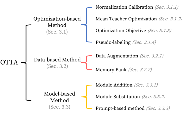
Figure 1: Taxonomy of existing OTTA methods. The categories, i.e., optimization-based, data-based, and model-based, inform three mainstream working mechanisms. Prompt-related methods are categorized into model-based methods.

Organization of the survey. The rest of this survey will be organized as follows. Sec. 2 presents the problem definition and introduces widely used datasets, metrics, and applications. Using the taxonomy shown in Fig. 1, Sec. 3 comprehensively reviews existing OTTA methods. Then, using transformer backbones, Sec. 4 empirically analyzes seven state-of-the-art methods based on new evaluation metrics on corrupted and real-world distribution shifts. We conclude the survey in Sec. 6.

2 Problem Overview

Online Test-time Adaptation (OTTA), with its online and real-time characteristics, represents a critical line of methods in test-time adaptation. This section providing a formal definition of OTTA and delving into its fundamental attributes. Furthermore, we explore widely used datasets and evaluation methods and examine the potential application scenarios of OTTA. A comparative analysis is undertaken to differentiate OTTA from similar settings to ensure a clear understanding.

2.1 Problem Definition

In OTTA, we assume access to a trained source model and adapt the model at test time over the test input before making the final prediction. The given source model $f_{\theta^{S}}$ parameterized by $\theta^{S}$ is pre-trained on a labeled source domain $\mathcal{D}_{S}=\{(\bm{x}^{S},\bm{y}^{S})\}$, which is formed by i.i.d. sampling from the source distribution $p_{S}$. Unlabeled test data $\mathcal{D}_{T}=\{\bm{x}_{1}^{T},\bm{x}_{2}^{T},\bm{x}_{t}^{T},\ldots,\bm{x}_{n}^{T}\}$ come in batches, where $t$ indicates the current time step, $n$ is the overall time steps (i.e., number of batches). Test data often come from one or multiple different distributions $(\bm{x}_{t}^{T},\bm{y}_{t}^{T})\sim p_{T}$, where $p_{S}(\bm{x},y)\neq p_{T}(\bm{x},y)$ under the covariate shift assumption (Huang et al, 2006). During TTA, we update the model parameters batch $t$, resulting in an adapted model $f_{\theta^{t}}$. Before adaptation, the pre-trained model is expected to retain its original architecture, including the backbone, without modifying its layers or introducing new model branches during training. Additionally, the model is restricted to observing the test data only once and must produce predictions promptly. By refining the definition of OTTA in this manner, we aim to minimize limitations associated with its application in real-world settings. Note that following adaptation to a specific domain, the model is reset to its original pretrained state. i.e., $\underline{f_{\theta^{S}}}\rightarrow f_{\theta^{0}}\rightarrow\underline{f_{\theta^{S}}}\rightarrow f_{\theta^{1}}\rightarrow\underline{f_{\theta^{S}}}\rightarrow\cdots f_{\theta^{t}}$.

Due to the covariate shift between the source and test data, adapting the source model without the source data poses a significant challenge. Since there is no way to align these two sets, one may ask, what kind of optimization objective could work under such a limited environment? Meanwhile, as the test data come at a fixed pace, how many could be a desirable amount to best fix the test-time adaptation? Or will the adaptation even work in the new era of backbones (e.g., ViTs)? Does “Test-time Adaptation” become a false proposition with the backbone upgrading? With these concerns, we unfold the OTTA methods by their datasets, evaluations, and applications and decouple their strategies, aiming to discover which one and why one component would work with the update of existing backbones.

2.2 Datasets

This survey mainly summarizes datasets in image classification, a fundamental problem in computer vision, while recognizing that OTTA has been applied to many downstream tasks (Ma et al, 2022; Ding et al, 2023; Saltori et al, 2022). Testbeds in OTTA usually seek to facilitate adaptation from natural images to corrupted ones. The latter are created by perturbations such as Gaussian noise and Defocus blur. Despite including corruptions at varying severities, these synthetically induced corruptions may not sufficiently mirror the authentic domain shift encountered in real-world scenarios. Our work uses corruption and real-world shift datasets, summarized in Table 1. Details of each testbed are described below.

• CIFAR-10-C is a standard benchmark for image classification. It contains 950,000 color images, each of 32x32 pixels, spanning ten distinct classes. CIFAR-10-C retains the class structure of CIFAR-10 but incorporates 15 diverse corruption styles, with severities ranging from levels 1 to 5. This corrupted variant aims to simulate realistic image distortions or corruptions that might arise during processes like image acquisition, storage, or transmission.

• CIFAR-100-C has 950,000 colored images with dimensions 32x32 pixels, uniformly distributed across 100 unique classes. The CIFAR-100 Corrupted dataset, analogous to CIFAR-10-C, integrates artificial corruptions into the canonical CIFAR-100 images.

• ImageNet-C is a corrupted version of ImageNet test set (Krizhevsky et al, 2012). Produced from ImageNet-1k, ImageNet-C has $19$ types of corruption domains, including $4$ validation corruptions. For each domain, $5$ levels of severity are produced, with $50,000$ images per severity from $1,000$ classes.

Although testbeds with corruptions have been extensively utilized, they might not fully capture the complexities of real-world scenarios as they represent artificially created domain differences. Experimental benchmarking from the real world is still lacking. Therefore, this paper evaluates OTTA on real-world test sets such as CIFAR-10-Warehouse and CIFAR-10.1 to address the limitations of such testbeds.

• CIFAR-10.1 (Recht et al, 2018) is a real-world test set with the same label space as CIFAR-10. It contains roughly 2,000 images sampled from the Tiny Image dataset (Yang et al, 2016).

• CIFAR-10-Warehouse (CIFAR-10-W) integrates images from both diffusion models, specifically Stable-diffusion-2-1 (Rombach et al, 2022), and targeted keyword searches across seven popular search engines. Comprising $37$ generated and $143$ real-world datasets, each subset has $300$ to $8,000$ images, revealing noticeable within-class variations across different search criteria.

2.3 Evaluation

Efficiency and accuracy are crucial for online test-time adaptation to reveal the efficiency of OTTA faithfully. This survey employs the following evaluation metrics:

Mean error (mErr) is one of the most commonly used metrics to assess model accuracy. It computes the average error rate across all corruption types or domains. While useful, this metric usually does not provide class-specific insights in OTTA.

GFLOPs refers to giga floating point operations per second, which quantifies the number of floating-point calculations a model performs in a second. A model with lower GFLOPs is more computationally efficient.

Number of updated parameters provides insights into the complexity of the adaptation process. A model that requires a large number of updated parameters may not be practical for online adaptation.

2.4 Relationship with Other Tasks

Offline test-time adaptation (TTA), also called source-free domain adaptation (Liang et al, 2020, 2022; Ding et al, 2022; Yang et al, 2021), is a technique to adapt a source pre-trained model to the target (i.e., test) set. This task assumes that the model can access the entire dataset multiple times. This differs from online test-time adaptation, where the test data is given in batches.

Continual TTA While OTTA requires resetting the adapted model back to the source pre-trained one for every distinct domain (i.e., corruption type), continual TTA (e.g., (Wang et al, 2022a; Hong et al, 2023; Song et al, 2023; Chakrabarty et al, 2023; Gan et al, 2023)) assumes no domain information available and does not allow any reset mechanism. Although the corruption domains in continuous TTA appear one by one, with clear boundaries between each domain, there is no separate indication of domain information during adaptation.

Gradual TTA tackles real-world scenarios where domain shifts are gradually introduced through incoming test samples (Marsden et al, 2022; Döbler et al, 2023). An example is the gradual and continuous change in weather conditions. For corruption datasets, existing gradual TTA approaches assume that test data transition from severity level 1 to level 2 and then progress slowly toward the highest level. Continual and gradual TTA methods also support online test-time adaptation (i.e., episodic learning).

Figure 2: Timeline of optimization-based OTTA methods.

Test-time Training (TTT) introduces an auxiliary task for both training and adaptation (Sun et al, 2020; Gandelsman et al, 2022). In the training phase, the original architecture, such as ResNet101 (He et al, 2016), is modified into a “Y”-shaped structure, where one task is image classification, and the other could be rotation prediction. During adaptation, the auxiliary task continues to be trained in a supervised manner so that model parameters are updated. The classification head output serves as the final prediction for each test sample.

Test-time augmentation (TTAug) applies data augmentations to input data during inference, resulting in multiple variations of the same test sample, from which predictions are obtained (Shanmugam et al, 2021; Kimura, 2021). The final prediction typically aggregates predictions of these augmented samples through averaging or majority voting. TTAug enhances model prediction performance by providing a range of data views. This technique can be applied to various tasks, including domain adaptation, offline TTA, and even OTTA, as TTAug does not require any modification of the model training process.

Domain generalization (Qiao et al, 2020; Wang et al, 2021b; Xu et al, 2021; Zhou et al, 2023) aims to train models that can perform effectively across multiple distinct domains without specific adaptation to any domain. It assumes the model learns domain-invariant features that are applicable across diverse datasets. While OTTA emphasizes dynamic adaptation to specific domains over time, domain generalization seeks to establish domain-agnostic representations. The choice between these strategies depends on the specific problem considered.

3 Online test-time adaptation

Given the distribution divergence of online data from source training data, OTTA techniques are broadly classified into three categories that hinge on their responses to two primary concerns: managing online data and mitigating performance drops due to distribution shifts. Optimization-based methods anchored in designing unsupervised objectives typically lean towards adjusting or enhancing pre-trained models. Model-based approaches look to modify or introduce particular layers. On the other hand, data-based methods aim to expand data diversity, either to improve model generalization or to harmonize consistency across data views. According to this taxonomy, we sort out existing approaches in Table 3 and review them in detail below.

3.1 Optimization-based OTTA

Optimization-based OTTA methods consist of three sub-categories: (1) recalibrating statistics in normalization layers, (2) enhancing optimization stability with the mean-teacher model, and (3) designing unsupervised loss functions. A timeline is illustrated in Fig. 2.

3.1.1 Normalization Calibration

In deep learning, a normalization layer aims to improve the training process and enhance the generalization capacity of neural networks by regulating the statistical properties of activations within a given layer. Batch normalization (BatchNorm) (Ioffe and Szegedy, 2015), as the most commonly used normalization layer, aims to stabilize the training process by its global statistics or a considerably large batch size. Operating by standardizing the mean and variance of activations, BatchNorm could also reduce the risk of vanishing or exploding gradients during training. There are also alternatives to BatchNorm, such as layer normalization (LayerNorm) (Ba et al, 2016), group normalization (GroupNorm) (Wu and He, 2020), and instance normalization (InstanceNorm) (Ulyanov et al, 2016) A similar idea to the normalization layer is feature whitening, which also adjusts features right after the activation layer. Both strategies are commonly used in domain adaptation literature (Roy et al, 2019; Carlucci et al, 2017).

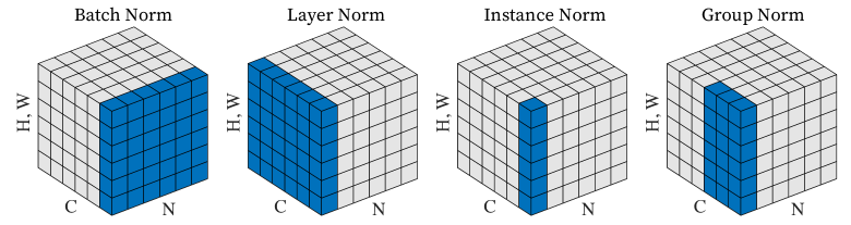
Figure 3: Visualizing normalization layers (Wu and He, 2020).

Example. Take the most commonly used BatchNorm as an example. Let $\bm{x}_{i}$ represent the activation for feature channel $i$ in a mini-batch. The BatchNorm layer will first calculate the batch-level mean $\bm{\mu}$ and variance $\bm{\sigma}^{2}$ by:

$$\quad\bm{\mu}=\frac{1}{m}\sum_{i=1}^{m}\bm{x}_{i},\quad\bm{\sigma}^{2}=\frac{1}{m}\sum_{i=1}^{m}(\bm{x}_{i}-\bm{\mu})^{2},$$ (1)

where $m$ is the mini-batch size. Then, the calculated statistics will be applied to standardize the inputs:

$$\quad\hat{\bm{x}}_{i}=\frac{\bm{x}_{i}-\bm{\mu}}{\sqrt{\bm{\sigma}^{2}+\epsilon}},\quad\bm{y}_{i}=\gamma\hat{\bm{x}}_{i}+\beta,$$ (2)

where $y_{i}$ is the final output of the $i$-th channel from this batch normalization layer, adjusting two learnable affine parameters, $\gamma$ and $\beta$. And $\epsilon$ is used to avoid division of $0$. For the update, the running mean $\bm{\mu}^{\text{run}}$ and variance $\sigma^{\text{run}}$ are computed as a moving average of the mean and variance over all batches seen during training, with a momentum factor $\alpha$:

$$~{}\bm{\mu}^{\text{run}}=\alpha\bm{\mu}+(1-\alpha)\bm{\mu}^{\text{run}},\quad\bm{\sigma}^{\text{run}}=\alpha\bm{\sigma}+(1-\alpha)\bm{\sigma}^{\text{run}}.$$ (3)

Motivation. In domain adaptation, aligning batch normalization statistics is shown to mitigate performance degradation brought by covariate shifts. The underlying hypothesis suggests that information about labels is encoded within the weight matrices of each layer. At the same time, knowledge related to specific domains is conveyed through the statistics of BatchNorm layer. Consequently, an adaptation based on updating BatchNorm layer could bring enhanced performance of unseen domains (Li et al, 2017). A similar idea can be used in online test-time adaptation. The assumption is, given a neural network $f$ trained on a source dataset $\mathcal{D}_{S}$ with normalization parameters $\beta$ and $\gamma$, updating $\{\gamma,\beta\}$ based on test data $\bm{x}_{i}^{t}$ at each time step $t$ will improve $f$’s robustness on the test domain. Building upon the assumption, initial investigations in OTTA predominantly revolved around fine-tuning only on updating the normalization layers. This strategy has a few popular variations. A common practice adjusts statistics ($\mu$ and $\sigma$) and affine parameters ($\beta$ and $\gamma$) in the BatchNorm layer. Note that the choice of normalization techniques, such as LayerNorm or GroupNorm, may depend on the backbone architecture and specific optimization objectives.

Tent (Wang et al, 2021a) and its subsequent works, such as (Niu et al, 2022; Jang et al, 2023), are representative approaches within this paradigm. They update the statistics and affine parameters of BatchNorm for each test batch while freezing the remaining parameters. However, as seen in Tent, updated by minimizing soft entropy, the effectiveness of batch-level updates is dependent on data quality within each batch, introducing potential performance fluctuations. For example, noisy or poisoned data with biased statistics would significantly influence the BatchNorm updates. Methods that aim at stabilization via dataset-level estimate are proposed to mitigate such performance fluctuation arising from batch-level statistics. Gradient preserving batch normalization GpreBN (Yang et al, 2022) is introduced that allows for cross instance gradient backpropagation by modifying the BatchNorm normalization factor:

$$\quad\hat{\bm{y}}_{i}=\frac{\frac{\bm{x}_{i}-\bm{\mu}_{c}}{\bm{\sigma}_{c}}\bar{\bm{\sigma}}_{c}+\bar{\bm{\mu}}_{c}-\bm{\mu}}{\bm{\sigma}}\gamma+\beta,$$ (4)

where $\frac{\bm{x}_{i}-\bm{\mu}_{c}}{\bm{\sigma}_{c}}$ is the standardized input feature $\hat{\bm{x}}_{i}$, same as in Eq. (2). $\bm{\sigma}_{c}$ and $\bm{\mu}_{c}$ means stop gradient. GpreBN normalizes $\hat{\bm{x}}_{i}$ by arbitrary non-learnable parameters $\bm{\mu}$ and $\bm{\sigma}$. MixNorm (Hu et al, 2021) mixies the statistics (produced by augmented sample inputs) of the current batch with the global statistics computed through moving average. Then, combining global-level and augmented batch-level statistics effectively bridges the gap between historical context and real-time fluctuations, enhancing performance regardless of batch size. As an alternative proposal, RBN (Yuan et al, 2023a) considers global robust statistics from a well-maintained memory bank with a fixed momentum of moving average when updating statistics to ensure high statistic quality. Similarly, Core (You et al, 2021) incorporates a momentum factor for moving average to fuse the source and test set statistics.

Instead of using a fixed momentum factor for the moving average, Mirza et al (2022) propose a dynamic approach. It determines the momentum of the moving average based on a decay factor. Assuming that model performance deteriorates over time, the decay factor should progressively be considered more from the current batch as time advances to avoid biased learning by misled source statistics. ERSK (Niloy et al, 2023) follows a similar idea but determines its momentum by the KL divergence of BatchNorm statistics between source-pretrained model and the current test batch.

Stabilization via renormalization. Merely emphasizing moving averages might undermine the inherent characteristics of gradient optimization and normalization when it comes to updating BatchNorm layers. As noted by Huang et al (2018), BatchNorm primarily centers and scales activations without addressing their correlation issue of activations, where a decorrelated activation can lead to better feature representation (Schmidhuber, 1992) and generalization (Cogswell et al, 2016). At the same time, batch size significantly influences correlated activations, which further brings limitations when batch size is small. Test-time batch renormalization module (TBR) in DELTA (Zhao et al, 2023a) addresses these limitations through a renormalization process. They adjust standardized outputs using two new parameters, $r$ and $d$. $r=\frac{sg\left(\hat{\bm{\sigma}}^{\text{batch }}\right)}{\hat{\bm{\sigma}}^{\text{ema }}}$ and $d=\frac{sg\left(\hat{\mu}^{\text{batch }}\right)-\hat{\bm{\mu}}^{\text{ema }}}{\hat{\bm{\sigma}}^{\text{ema }}}$, where $sg(\cdot)$ is stop gradient. Both parameters are computed using batch and global moving statistics, using a novel approach to maintaining stable batch statistics updating strategies (inspired by (Ioffe, 2017)). Then $\hat{\bm{x}}_{i}$ is normalized further by $\hat{\bm{x}}_{i}=\hat{\bm{x}}_{i}\cdot r+d$. The above OTTA methods reset the model for each domain; this limits the model applicability to scenarios that commonly have no clear domain boundary during adaptation. NOTE (Gong et al, 2022) focuses on continual OTTA under temperal correlaton, i.e., distribution changes over time $t$: $\left(\mathbf{x}_{t},\bm{y}_{t}\right)\sim P_{\mathcal{T}}(\mathbf{x},\bm{y}\mid t)$. Authors propose instance-level BatchNorm to avoid potential instance-wise variations in a domain non-identifiable paradigm.

Stabilization via enlarging batches. To improve the stability of adaptation, another idea is using large batch sizes. In fact, most methods based on batch normalization employ substantial batch sizes such as $200$ in (Wang et al, 2021a; Hu et al, 2021). Despite its effectiveness, this practice cannot deal with scenarios where data arrives in smaller quantities due to hardware (e.g., GPU memory) constraints, especially in edge devices.

Alternatives to Batchnorm. To avoid using large-sized batches, viable options include updating GroupNorm (Mummadi et al, 2021) or LayerNorm, especially in transformer-based tasks (Kojima et al, 2022). The former method uses entropy for updating, while the latter further requires the assistance of sharpness-aware minimization (Foret et al, 2021) in (Niu et al, 2023), which seeks a flat minimum of optimization. Followed by the above situation in scenarios where computational resources are limited, MECTA (Hong et al, 2023) introduced an innovative approach by replacing the conventional BatchNorm layer with a customized MECTA norm. This strategic change effectively mitigated memory usage concerns during adaptation, reducing the memory overhead associated with large batch sizes, extensive channel dimensions, and numerous layers requiring updates. Taking a different tack, EcoTTA (Song et al, 2023) incorporated and exclusively updated meta networks, including BatchNorm layers. This approach also effectively curtailed computational expenses, keeping source data discriminability while upholding robust test-time performance. Furthermore, to address the performance challenges associated with smaller batch sizes, TIPI (Nguyen et al, 2023) introduced additional BatchNorm layers in conjunction with the existing ones. This configuration inherently maintains two distinct sets of data statistics and leverages shared affine parameters to enhance consistency across different views of test data.

3.1.2 Mean Teacher Optimization

The mean teacher model, as discussed in (Tarvainen and Valpola, 2017), presents a viable strategy to enhance optimization stability in OTTA. This approach involves initializing both the teacher and student models with a pre-trained source model. For any given test sample, weak and strong augmented versions are created. Each version is then processed by the student and teacher model correspondingly. The crux of this approach lies in employing prediction consistency, also known as consistency regularization, to update the student model. This strategy aims to achieve identical predictions from different data views, thereby reducing model sensitivity to the changes in the test data and improving prediction stability. Simultaneously, the teacher model is refined as a moving average of the student across iterations. Notably, in OTTA, the mean teacher model and BatchNorm-based methods are not mutually exclusive; in fact, they can be effectively integrated. Incorporating BatchNorm updates into the teacher-student learning framework can yield even more robust results (Sec. 4). Similarly, the integration of the mean-teacher model with data-driven (as discussed in Sec. 3.2) or model-driven (as detailed in Sec. 3.3) methods shows promise for further enhancing the prediction accuracy and stability of OTTA, marking an important step forward in the field.

Model updating strategies. Following the idea of mean-teacher learning, ViDA (Liu et al, 2023b) utilizes to supervise the student output by the prediction from the teacher with augmented input. It further introduces high/low-rank adapters to be updated to suit continual OTTA learning. Details see Sec. 3.3. Wang et al (2022a) generally follows the standard consistency learning strategy but introduces a reset method: a fixed number of weights are reset to their source pre-trained states after each training iteration. This reset measure preserves source knowledge and brings robustness against misinformed updates.

RoTTA (Yuan et al, 2023a) adopts a different approach, focusing on updating only the customized batch normalization layer, termed RBN, in the student model, rather than altering all parameters. This strategy not only benefits from consistency regularization but also integrates statistics of the out-of-distribution test data.

Divergence in Augmentations. Drawing inspiration from the prediction consistency strategy in the mean teacher model, Tomar et al (2023) propose learning adversarial augmentation to identify the most challenging augmentation policies, which drive image feature representations of towards uncertain regions near decision boundaries. This method not only achieves clearer decision boundaries but also enhances the separation of class-specific features, significantly improving model insensitivity to styles of unseen test data.

3.1.3 Optimization Objective

Designing a proper optimization objective is important under the challenges of shifted test data with a limited amount. Commonly seen optimization-based Online Test-time Adaptation (OTTA) are summarized in Fig. 4. Existing literature addresses the optimization problem using three primary strategies below.

Optimizing (increasing) confidence. Covariate shifts typically lead to lower model accuracy, which in turn causes the model to express high uncertainty. The latter is often observed As such, to improve model performance, an intuitive way is to enhance model confidence for the test data.

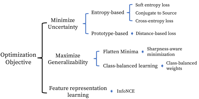
Figure 4: Common optimization objectives in OTTA.

Entropy-based confidence optimization. This strategy typically aims to minimize the entropy of the softmax output vector:

$$\quad H(\hat{y})=-\sum_{c}p\left(\hat{y}_{c}\right)\log p\left(\hat{y}_{c}\right),$$ (5)

where $\hat{y}_{c}$ is the $c$-th predicted class, $p\left(\hat{y}_{c}\right)$ is its corresponding prediction probability. Intuitively, when the entropy of the prediction decreases, the vector will look sharper, where the confidence, or maximum confidence, increases. In OTTA, this optimization method will increase model confidence for the current batch without replying to labels and improve model accuracy.

Two lines of work exist. One considers the entire softmax vector; the other leverages auxiliary information and uses the maximum entry of the softmax output. Tent is a typical method for the former.

Tent is a popular method that uses entropy minimization to update the affine parameters in BatchNorm. Subsequent studies have adopted and expanded upon this strategy. For example, EATA (Niu et al, 2022) implements a sample selection strategy on top of entropy minimization by only updating reliable and unique samples. Following EATA, Seto et al (2023) introduces entropy minimization by incorporating self-paced learning. This addition ensures the learning process progresses at an adaptive and optimal pace. Furthermore, by integrating the general adaptive robust loss (Barron, 2019) into self-paced learning, the proposed method achieves robustness against large and unstable loss values. TTPR (Sivaprasad et al, 2021) combines entropy minimization with prediction reliability, which operates across various views of a test image to form a consistency loss. This is done by merging the mean prediction across three augmented versions, with each augmented prediction separately. Lin et al (2023) introduces minimizing the entropy loss on augmentation-averaged predictions while assigning high weights for low-entropy samples. In SAR (Niu et al, 2023), when minimizing entropy, an optimization strategy is used so that parameters enabling ‘flatter’ minimum regions can be found. This is shown to allow for a better model updating stability.

While entropy minimization is widely used, a natural question arises: what makes soft entropy a preferred choice? To reveal the working mechanism of the loss function, Conj-PL (Goyal et al, 2022) designs a meta-network to parameterize it and observes that the meta-output could echo the temperature-scaled softmax output of a given model. They prove that if the cross-entropy loss is applied during source pre-training, the soft entropy loss is the most proper loss during adaptation.

A drawback of entropy minimization is the overly early convergence because gradients of high-confidence predictions do not contribute much. To allow contributions from reliable predictions and thus smooth updating, SLR (Mummadi et al, 2021) borrows the negative log-likelihood ratio NLLR(Zhu et al, 2018)

$$R\left(\hat{y},y^{r}\right)=-\sum_{c}y_{c}^{r}\log\frac{\hat{y}_{c}}{\sum_{i\neq c}\hat{y}_{i}}$$ (6)

$$=H\left(\hat{y},y^{r}\right)+\sum_{c}y_{c}^{r}\log\sum_{i\neq c}\hat{y}_{i},$$

to design their loss. Here, $\hat{y}$ is the prediction that wants to approach $y^{r}$, and $c$ is the predicted class. The entropy $H$ is lower bound by $0$. Even if $y_{c}^{r}\rightarrow 1$ and $\sum_{i\neq c}\hat{y}_{i}\rightarrow 0$, where traditional entropy minimization occurs the gradient vanishing issue for high-confidence predictions, NLLR could induce non-vanishing gradients since $\log\sum_{i\neq c}\hat{y}_{i}\rightarrow-\infty$.

Another drawback of entropy minimization is that it might obtain a degenerate solution where every data point is assigned to the same class. To avoid this, MuSLA (Kingetsu et al, 2022) employs mutual information of the sample $X$ and the corresponding prediction $\hat{Y}$,

$$\quad I_{t}(X;\hat{Y})=H\left(\hat{\bm{p}}_{0}\right)-\frac{1}{\mathbf{M}}\sum_{t^{i}}H\left(\hat{\bm{p}_{t}^{i}}\right),$$ (7)

where $\hat{\bm{p}}_{0}$ is the prior distribution, $M$ is mini-batch size, $i$ is the index of the sample within the batch. Maximizing $\frac{1}{\mathbf{M}}\sum_{t^{i}}H\left(\hat{\bm{p}_{t}^{i}}\right)$ could be seen as a regularizer to avoid same-class prediction.

The cooperation between a teacher and a student is another possible solution to optimize prediction confidence with reliability. Here, the teacher is usually the moving average of the model of interest across iterations. CoTTA (Wang et al, 2022a) uses the Softmax prediction from the teacher to supervise the Softmax predictions from the student under the cross-entropy loss.

To give more precise supervision to the student, RoTTA (Yuan et al, 2023b) adds a twist: the model is updated using samples stored in a memory bank. Moreover, a reweighting mechanism is introduced to prevent the model from overfitting to ‘old’ samples in the memory bank. This reweighting prioritizes updates using ‘new’ samples in the memory bank, ensuring a more dynamic and current learning process. Please see Sec. 3.2.2 for more details about its memory bank strategy.

Supervised by student output, TeSLA design its objective as a cross-entropy loss with a regularizer:

$$\mathcal{L}_{\mathrm{pl}}(\bm{X},\hat{\bm{Y}})=-\frac{1}{B}\sum_{i=1}^{B}\sum_{k=1}^{K}f_{s}\left(\bm{x}_{i}\right)_{k}\log\left(\left(\hat{\bm{y}}_{i}\right)_{k}\right)$$ (8)

$$+\sum_{k=1}^{K}\hat{f}_{s}(\bm{X})_{k}\log\left(\hat{f}_{s}(\bm{X})\right)_{k},$$

where $\hat{f}_{s}(X)=\frac{1}{B}\sum_{i=1}^{B}f_{s}\left(\bm{x}_{i}\right)$ is the marginal class distribution of the student over the batch. $\hat{y}$ is the soft pseudo-label from the teacher model. $k$ is the number of classes. Except for the cross-entropy loss similar to the previous methods, it also maximizes the entropy for the averaged prediction of the student model across the batch to avoid overfitting.

A cross-entropy loss helps minimize model prediction uncertainty but may fail to give consistent uncertainty scores under different augmentations, model randomness (MC dropout), etc. This problem is more critical when the teacher-student mechanism is not used. To address this problem, MEMO (Zhang et al, 2022) computes the average prediction across multiple augmentations for each test sample and then minimizes the entropy of the marginal output distribution over augmentations:

$$\ell(\theta;\mathbf{x})\triangleq H\left(\bar{p}_{\theta}(\cdot\mid\mathbf{x})\right)=-\sum_{y\in\mathcal{Y}}\bar{p}_{\theta}(y\mid\mathbf{x})\log\bar{p}_{\theta}(y\mid\mathbf{x}),$$ (9)

where $\bar{p}$ denotes the averaged Softmax vector. Here, augmentations are randomly generated by AugMix (Hendrycks et al, 2020).

Prototype-based optimization. Prototype-based learning (Yang et al, 2018) is a commonly used strategy for unlabeled data by selecting representative or average for each class and classifying unlabeled data by distance-based metrics. However, its effectiveness might be limited under distribution shifts. Seeking a reliable prototype, TSD (Wang et al, 2023) uses a Shannon entropy-based filter to find class prototypes from target samples that have high confidence. Then, a target sample is used to update the classifier-of-interest if its nearest prototypes are consistent with its class predictions from the same classifier.

Improving generalization ability to unseen target samples. Typically, OTTA uses the same batch of data for model update and evaluation. Here, we would like the model to perform well on upcoming test samples or have good generalization ability. A useful technique is sharpness-aware minimization (SAM) (Foret et al, 2021), where instead of seeking a minima that is ‘sharp’ in its gradients nearby, a ‘flat’ minima region is preferred. Niu et al (2023) uses the following formulation to demonstrate the effectiveness of this strategy.

$$\quad\min_{\tilde{\Theta}}S(\mathbf{x})E^{SA}(\mathbf{x};\Theta).$$ (10)

Here, $S(\mathbf{x})$ is an entropy-based indicator function that can filter out unreliable predictions based on a predefined threshold. $E^{SA}(\mathbf{x};\Theta)$ is defined as:

$$\quad E^{SA}(\mathbf{x};\Theta)\triangleq\max_{\|\epsilon\|_{2}\leq\rho}E(\mathbf{x};\Theta+\bm{\epsilon}).$$ (11)

This term aims to identify a weight perturbation $\epsilon$ within a Euclidean ball of radius $\rho$ that maximizes entropy. It quantifies sharpness by measuring the maximal change in entropy between $\Theta$ and $\Theta+\rho$. As such, Eq. 11 jointly minimizing entropy and its sharpness. Gong et al (2023) uses same idea for their optimization.

Another difficulty affecting OTTA generalization is the class imbalance in a batch: a limited number of data for the model update would often not reflect the true class frequency. To solve this problem, Dynamic online re-weighting (DOT) in DELTA (Zhao et al, 2023a) uses a momentum-updated class-frequency vector, which is initialized with equal weights for each class and then updated at every inference step based on the pseudo-label of the current sample and model weight. For a target sample, a significant weight (or frequency) for a particular class prompts DOT to diminish its contribution during subsequent adaptation learning, which avoids biased optimization towards frequent classes, thus improving model generalization ability.

Feature representation learning. Since no annotations are assumed for the test data, contrastive learning (van den Oord et al, 2018) could naturally be used in test-time adaptation tasks. In a self-supervised fashion, contrastive learning is to learn a feature representation where positive pairs (data sample and its augmentations) are close and negative pairs (different data samples) are pushed away from each other. However, this requires multiple-epoch updates, which violate the online adaptation setting. To suit online learning, AdaContrast (Chen et al, 2022) uses target pseudo-labels to disregard the potential same-class negative samples rather than treat all other data samples as negative.

3.1.4 Pseudo-labeling

Pseudo-labeling is a useful technique in domain adaptation and semi-supervised learning. It typically assigns labels to samples with high confidence, and these pseudo-labeled samples are then used for training.

In OTTA, where adaptation is confined to the current batch of test data, batch-level pseudo-labeling is often used. For example, MuSLA (Kingetsu et al, 2022) implements pseudo-labeling as a post-optimization step following BatchNorm updates. This approach refines the classifier using pseudo-labels of the current batch, thereby enhancing model accuracy.

Furthermore, the teacher-student framework, as seen in models like CoTTA (Wang et al, 2022a), RoTTA (Yuan et al, 2023b), and ViDA (Liu et al, 2023b), also adopts the pseudo-labeling strategy where the teacher outputs are used as soft pseudo-labels. With the uncertainty maintained during backpropagation, this could prevent the model from being overfitted to the incorrect predictions.

Reliable pseudo labels are an essential requirement. However, it is particularly challenging in the context of OTTA. On the one hand, due to the use of continuous data streams, we have limited opportunity for review. On the other hand, the covariate shift between the source and test sets could significantly degrade the reliability of pseudo-labels.

To address these challenges, TAST (Jang et al, 2023) adopts a prototype-based pseudo-labeling strategy. They first obtain the prototypes as the class centroids in the support set, where the support set is initially derived from the weights of the source pre-trained classifier and then refined and updated using the normalized features of the test data. To avoid performance degradation brought by unreliable pseudo labels, it calculates centroids only using the nearby support examples and then uses the temperature-scaled output to obtain the pseudo labels. Alternatively, AdaContrast (Chen et al, 2022) uses soft $K$ nearest neighbors voting (Mitchell and Schaefer, 2001) in the feature space to generate reliable pseudo labels for target samples. On the other hand, Wu et al (2021) proposes to use multiple augmentations and majority voting to achieve consistent and trustworthy pseudo-labels.

Complementary pseudo-labeling (PL). One-hot pseudo-labels often result in substantial information loss, especially under domain shifts. To address this, ECL (Han et al, 2023) considers both maximum-probability predictions and predictions that fall below a certain confidence threshold (i.e., complementary labels). This is because of the intuition that if the model is less confident about a prediction, this prediction should be penalized more heavily. This method helps prevent the model from making aggressive updates based on incorrect but high-confidence predictions, offering a more stable approach similar to soft pseudo-label updates.

3.1.5 Other Approaches

Deviating from the conventional path of adapting source pre-trained models, Laplacian Adjusted Maximum likelihood Estimation (LAME) (Boudiaf et al, 2022) focuses on refining the model output. This is achieved by discouraging the refined output from deviating from the pre-trained model while encouraging label smoothness according to the manifold smoothness assumption. The final refined prediction is obtained when the energy gap for each refinement step of a batch is small.

3.1.6 Summary

Optimization-based methods stand out as the most commonly seen category in online test-time adaptation, independent of the neural architecture. These methods concentrate on ensuring consistency, stability, and robustness in optimization. However, an underlying assumption of these methods is the availability of sufficient target data, which should reflect the global test data distribution. Addressing this aspect, the next section will focus on data-based methods, examining how they tackle the lack of accessible target data in OTTA.

3.2 Data-based OTTA

With a limited number of samples in the test batch, it is common to encounter test samples with unexpected distribution changes. We acknowledge data might be the key to bridging this gap between the source and the test data. In this section, we delve deeper into strategies centered around data in OTTA. We highlight various aspects of data, such as diversifying the data in each batch (Sec. 3.2.1) and preserving high-quality information on a global scale (Sec. 3.2.2). These strategies could enhance model generalizability and tailor model discriminative capacity to the current data batch.

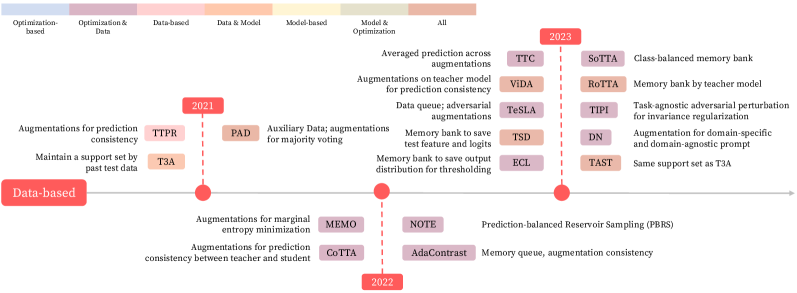
Figure 5: Timeline of Data-based OTTA methods.

3.2.1 Data Augmentation

Data augmentation is important in domain adaptation (Wang and Deng, 2018) and domain generalization (Zhou et al, 2023), which mimics real-world variations to improve model transferability and generalizability. It is particularly useful for test-time adaptation.

Predefined augmentations. Common data augmentation methods like cropping, blurring, and flipping are effectively incorporated into various OTTA methodologies. An example of this integration is TTC (Lin et al, 2023), which updates the model using averaged predictions from multiple augmentations. Another scenario is from the mean teacher model such as RoTTA (Yuan et al, 2023b), CoTTA (Wang et al, 2022a), and ViDA (Liu et al, 2023b), applies predefined augmentations to teacher/student input, and maintains prediction consistency across different augmented views.

To ensure consistent and reliable predictions, PAD (Wu et al, 2021) employs multiple augmentations of a single test sample for majority voting. This is grounded in the belief that if the majority of the augmented views yield the same prediction, it is likely to be correct, as it demonstrates insensitivity to variations in style. Instead, TTPR (Sivaprasad et al, 2021) adopts KL divergence to achieve consistent predictions. For every test sample, it generates three augmented versions. The model is then refined by aligning the average prediction across these augmented views with the prediction for each view. Another approach is MEMO, which uses AugMix (Hendrycks et al, 2020) for test images. For a test data point, a range (usually $32$ or $64$) of augmentations from the AugMix pool $\mathcal{A}$ is generated to make consistent predictions.

Contextual Augmentations. Previously, OTTA methods often predetermine augmentation policies. Given that test distributions can undergo substantial variations in continuously evolving environments, there exists a risk that such fixed augmentation policies may not be suitable for every test sample. In CoTTA (Wang et al, 2022a), rather than augmenting every test sample by a uniformed strategy, augmentations are judiciously applied only when domain differences (i.e., low prediction confidence) are detected, mitigating the risk of misleading the model.

Adversarial Augmentation. Traditional augmentation methods always provide limited data views without fully representing the domain differences. TeSLA (Tomar et al, 2023) moves away from this. It instead leverages adversarial data augmentation to identify the most effective augmentation strategy. Instead of a fixed augmentation set, it creates a policy search space $\mathcal{O}$ as the augmentation pool, then assigns a magnitude parameter $m\in[0,1]$ for each augmentation. A sub-policy $\rho$ consists of augmentations and their corresponding magnitudes. To optimize the policy, the teacher model is adapted using an entropy maximization loss with a severity regularization to encourage prediction variations while avoiding the augmentation too strong to be far from the original image.

3.2.2 Memory Bank

Going beyond augmentation strategies that could diversify the data batch, the memory bank is a powerful tool to preserve valuable data information for future memory replay. Setting up a memory bank involves two key considerations: (1). Determining which data should be stored in the memory bank. This requires identifying samples that are valuable for possible replay during adaptation. (2). The management of the memory bank. This includes strategies for adding new instances and removing old ones from the bank.

Memory bank strategies generally fall into time-uniform and class-balanced categories. Notably, many methods choose to integrate both types to maximize effectiveness. In addressing the challenges posed by both temporally correlated distributions and class-imbalanced issues, NOTE (Gong et al, 2022) introduces the Prediction-Balanced Reservoir Sampling (PBRS) to save sample-prediction pairs. The ingenuity of PBRS lies in its fusion of two distinct sampling strategies: time-uniform and prediction-uniform. The time-uniform approach, reservoir sampling (RS), aims to obtain uniform data over a temporal stream. Specifically, for a sample $x$ being predicted as class $k$, we randomly sample a value $p$ from a uniform distribution $[0,1]$. Then, if $p$ is smaller than the proportion of class $k$ in whole memory bank samples, pick one randomly from the same class and replace it with the new one $x$. Instead, the prediction-uniform saving strategy (PB) prioritizes the predicted labels to ascertain the majority class within the memory. Upon identification, it supplants a randomly selected instance from the majority class with a fresh data sample, thereby ensuring a balanced representation. The design of PBRS ensures a more harmonized distribution of samples across both time and class dimensions, fortifying the model’s adaptation capabilities.

A similar strategy is employed in SoTTA (Gong et al, 2023) to facilitate class-balanced learning. Each high-confidence sample-prediction pair is stored when the memory bank has available space. If the bank is full, the method opts to replace a sample either from one of the majority classes or from its class if it belongs to the majority. This ensures a more equitable class distribution and strengthens the learning process against class imbalances. Another work, RoTTA (Yuan et al, 2023b), offers a category-balanced sampling with timeliness and uncertainty (CSTU) module, dealing with the batch-level shifted label distribution. In CSTU, the author proposes a category-balanced memory bank $M$ with a capacity of $N$. In the memory bank, data samples $x$ are stored alongside their predicted labels $\hat{y}$, a heuristic score $\mathcal{H}$, and uncertainty metrics $\mathcal{U}$. Here, the heuristic score is calculated by:

$$\quad\mathcal{H}=\lambda_{t}\frac{1}{1+\exp(-\mathcal{A}/\mathcal{N})}+\lambda_{u}\frac{\mathcal{U}}{\log\mathcal{C}}$$ (12)

where $\lambda_{t}$ and $\lambda_{u}$ is the trade-off between time and uncertainty, $\mathcal{A}$ is the age (i.e., how many iterations this sample has been stored in the memory bank) of a sample stored in the memory bank. $\mathcal{C}$ is the number of classes, $\mathcal{N}$ is the capacity of the memory bank, and $\mathcal{U}$ is the uncertainty measurement, which is implemented as the entropy of the sample prediction. The score $\mathcal{H}$ is then used to decide whether a test sample should be saved into the memory bank for each class. As the lower heuristic score is always preferred, its intuition is to maintain fresh (i.e., lower age $\mathcal{A}$), balanced, and certain (i.e., lower $\mathcal{U}$) test samples. thereby enhancing adaptability during online operations.

To avoid the negative impact of the batch-level class distribution, TeSLA (Tomar et al, 2023) incorporates an online queue to hold class-balanced, weakly augmented sample features and their corresponding pseudo-labels. To enhance the correctness of pseudo-label predictions, each test sample is compared with its closest matches within the queue. Similarly, TSD (Wang et al, 2023) is dedicated to preserving sample embeddings and their associated logits in a memory bank for trustworthy predictions. Initialized by the weights from a source pre-trained linear classifier (Iwasawa and Matsuo, 2021), this memory bank is subsequently employed for prototype-based classification.

Contrastive learning is well-suited for OTTA, as discussed in 3.1.3. However, this approach can be challenging for online learning, especially when it pushes away feature representations of data from the same class. Unlike conventional methods where the feature space can be revisited multiple times, AdaContrast (Chen et al, 2022) offers an innovative solution. It keeps all previously encountered key features and pseudo-labels in a memory queue to avoid forming ’push-away’ pairs from the same class. This method speeds up the learning process and reduces the risk of error accumulation in data from the same class, thereby improving the efficiency and precision of the learning process.

ECL (Han et al, 2023) represents a novel shift away from traditional methods by incorporating a memory bank about output distributions for setting thresholds on complementary labels. The memory bank is also periodically refreshed using the newly updated model parameters, ensuring its relevance and effectiveness.

3.2.3 Summary

Data-based techniques are particularly useful for handling online test sets that may be biased or have unique stylistic constraints. However, these techniques often increase computational demands, posing challenges in online scenarios. The following section will focus on an alternative strategy: how architectural modifications can offer distinct advantages in Online Test-Time Adaptation.

3.3 Model-based OTTA

Model-based OTTA concentrates on adjusting the model architecture to address distribution shifts. The changes made to the architecture generally involve either adding new components or replacing existing blocks. This category is expanded to include developments in prompt-based techniques. It involves adapting prompt parameters or using prompts to guide the adaptation process.

3.3.1 Module Addition

Figure 6: Timeline of Model-based OTTA methods.

Input Transformation. In an effort to counteract domain shift, Mummadi et al (2021) introduce to optimize an input transformation module $d$, along with the BatchNorm layers as discussed in Sec. 3.1.3. This module is built on the top of the source model $f$, i.e., $g=f\circ d$. Specifically, $d(x)$ is defined as:

$$\quad d(x)=\gamma\cdot[\tau x+(1-\tau)r_{\psi}(x)]+\beta,$$ (13)

where $\gamma$ and $\beta$ are channel-wise affine parameters. The component $r_{\psi}$ denotes a network designed to have the same input and output shape, featuring $3\times 3$ convolutions, group normalization, and ReLU activations. The parameter $\tau$ facilitates a convex combination of the unchanged and transformed input $r_{\psi}(x)$.

Adaptation Module. To stabilize predictions during model updates, TAST (Jang et al, 2023) integrates $20$ adaptation modules to the source pre-trained model. Based on BatchEnsemble (Wen et al, 2020), these modules are appended to the top of the pre-trained feature extractor. The adaptation modules are updated multiple times independently by merging their averaged results with the corresponding pseudo-labels for a batch of data.

In the case of continual adaptation, promptly detecting and adapting to changes in data distribution is inevitable to deal with catastrophic forgetting and the accumulation of errors. To realize this, ViDA (Liu et al, 2023b) utilizes the idea of low/high-rank feature cooperation. Low-rank features retain general knowledge, while high-rank features better capture distribution changes. To obtain these features, the authors introduce two adapter modules correspondingly parallel to the linear layers (if the backbone model is ViT). Additionally, since distribution changes in continual OTTA are unpredictable, strategically combining low/high-rank information is crucial. Here, the authors use MC dropout (Gal and Ghahramani, 2016) to assess model prediction uncertainty about input $x$. This uncertainty is then used to adjust the weight given to each feature. Intuitively, if the model is uncertain about a sample, the weight of domain-specific knowledge (high-rank feature) is increased, and conversely, the weight of domain-shared knowledge (low-rank feature) is increased. This helps the model dynamically recognize distribution changes while preserving its decision-making capabilities.

3.3.2 Module Substitution

Layer substitution typically refers to swapping an existing layer in a model with a new one. The commonly used techniques are about:

Classifier. Cosine-distance-based classifier (Chen et al, 2009) offers great flexibility and interpretability by leveraging similarity to representative examples for decision-making. Employing this, TAST (Jang et al, 2023) formulates predictions by assessing the cosine distance between the sample feature and the support set. TSD (Wang et al, 2023) employs a similar classifier, assessing the features of the current sample against those of its K-nearest neighbors from a memory bank. PAD (Wu et al, 2021) uses a cosine classifier for predicting augmented test samples in its majority voting process. T3A (Iwasawa and Matsuo, 2021) relies on the dot product between templates in the support set and input data representations for classification.

In the context of updating BatchNorm statistics, any alteration to BatchNorm that extends beyond the standard updating approach can be classified under this category. This includes techniques such as MECTA norm (Hong et al, 2023), MixNorm (Hu et al, 2021), RBN (Yuan et al, 2023a), and GpreBN (Yang et al, 2022), etc. To maintain focus and avoid redundancy, these specific methods and their intricate details will not be extensively covered again in this section.

3.3.3 Prompt-based Method

The rise of vision-language models demonstrates their remarkable ability in zero-shot generalization. However, these models often underperform for domain-specific data. While attempting to address this, traditional fine-tuning strategies typically compromise the model’s generalization power by altering its parameters.

In response, borrows the idea from test-time adaptation, Test Time Prompt Tuning emerges as a solution. Deviating from the conventional methods, it fine-tunes the prompt, adjusting only the context of the model’s input, thus preserving the generalization power of the model. One representative is TPT (Shu et al, 2022). It generates $N$ randomly augmented views of each test image and updates the prompting parameter by minimizing the entropy of the averaged prediction probability distribution. Additionally, a confidence selection strategy is proposed to filter out the output with high entropy to avoid noisy updating brought by unconfident samples. By updating the learnable parameter of the prompt, it could be easier to adapt the model to the new, unseen domains.

(a) CIFAR-10-C $\&$ 10.1 Dataset

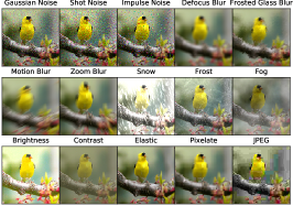
(b) ImageNet-C Dataset

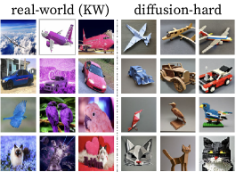
(c) CIFAR-10-Warehouse Dataset

Figure 7: The exemplars of the adopted datasets. The datasets include color variations, synthetic data, and types of corruption.

The prompt-related ideas are also powerful in OTTA tasks. “Decorate the Newcomers” (DN) (Gan et al, 2023) employs prompts as supplementary information added onto the image input. To infuse the prompts with relevant information, it employs a student-teacher framework in conjunction with a frozen source pre-trained model to capture both domain-specific and domain-agnostic prompts. For acquiring domain-specific knowledge, it optimizes the cross-entropy loss between the outputs of the teacher and student models. Additionally, DN introduces a parameter insensitivity loss to mitigate the impact of parameters prone to domain shifts. This strategy aims to ensure that the updated parameters, which are less sensitive to domain variations, effectively retain domain-agnostic knowledge. Through this approach, DN balances learning new, domain-specific information while preserving crucial, domain-general knowledge.

Gao et al (2022) introduces a novel method (DePT). Its process starts by segmenting the transformer into multiple stages, then introducing learnable prompts at the initial layer of each stage, concatenated with image and CLS tokens. During adaptation, DePT utilizes a mean-teacher model to update the learnable prompts and the classifier in the student model. For the student model, updates are made based on the cross-entropy loss calculated between pseudo labels and outputs from strongly augmented student output. Notably, these pseudo labels are generated from the student model, using the averaged predictions of the top-k nearest neighbors of the student’s weakly augmented output within a memory bank. In terms of the teacher-student interaction, to counter potential errors from incorrect pseudo labels, DePT implements an entropy loss between predictions made by strongly augmented views of both the student and teacher models. Additionally, the method minimizes the mean squared error between the combined prompts of the student and teacher models at the output layer of the Transformer. Furthermore, to ensure that different prompts focus on diverse features and to prevent trivial solutions, DePT also maximizes the cosine distance among the combined prompts of the student.

3.3.4 Summary

Model-based OTTA methods have shown effectiveness but are less prevalent than other groups, mainly due to their reliance on particular backbone architectures. For example, layer substitution mainly based on BatchNorm in the model makes them inapplicable to ViT-based architectures.

A critical feature of this category is its effective integration with prompting strategies. This combination allows for fewer but more impactful model updates, leading to greater performance improvements. Such efficiency makes model-based OTTA methods especially suitable for complex scenarios.

4 Empirical Study

In this empirical study, we focus on upgrading existing OTTA methods for the Vision Transformer (ViT) model (Dosovitskiy et al, 2021), investigating their potential to migrate to new generations of backbones. We provide solutions for adapting methods originally proposed for the CNN architecture to ViTs.

Baselines. We benchmark seven OTTA methods. To ensure fairness, we adhere to a standardized testing protocol and select five datasets, including three corrupted ones (i.e., CIFAR-10-C, CIFAR-100-C, and ImageNet-C), one real-world shifted dataset (CIFAR-10.1), and one comprehensive dataset (CIFAR-10-Warehouse). The CIFAR-10-Warehouse repository plays a crucial role in our evaluation, offering a wide range of subsets, including real-world variations sourced from different search engines and images generated through diffusion processes. Specifically, our survey focuses on two subsets of the CIFAR-10-Warehouse dataset: the Google split and the Diffusion split. These subsets, embodying both real-world and artificial data shifts, facilitate a comprehensive assessment of OTTA methods.

4.1 Implementation Details

Optimization details. We employ PyTorch for implementation. The foundational backbone for all approaches is ViT-base-patch16-224 (Dosovitskiy et al, 2021). When using CIFAR-10-C, CIFAR-10.1, and CIFAR-10-Warehouse as target domains, we train the source model on CIFAR-10 with $8,000$ iterations, including a warm-up phase spanning 1,600 iterations. The training uses a batch size 64 and the stochastic gradient descent (SGD) algorithm with a learning rate of $3e-2$. We mostly use an identical configuration to train the source model on CIFAR-100, with an extended training duration of $16,000$ iterations and a warm-up period spanning $4,000$ iterations. The source model on the ImageNet-1k dataset is acquired from the Timm repository . Additionally, we apply basic data augmentation techniques, including random resizing and cropping, across all methods. The Adam optimizer with a momentum term $\beta$ of $0.9$ and a learning rate of $1e-3$ ensures consistency during adaptation. Resizing and cropping techniques are applied as a default preprocessing step for all datasets. Then, a uniform normalization $(0.5,0.5,0.5)$ is adopted to mitigate potential performance fluctuations arising from external factors beyond the algorithm’s core operations.

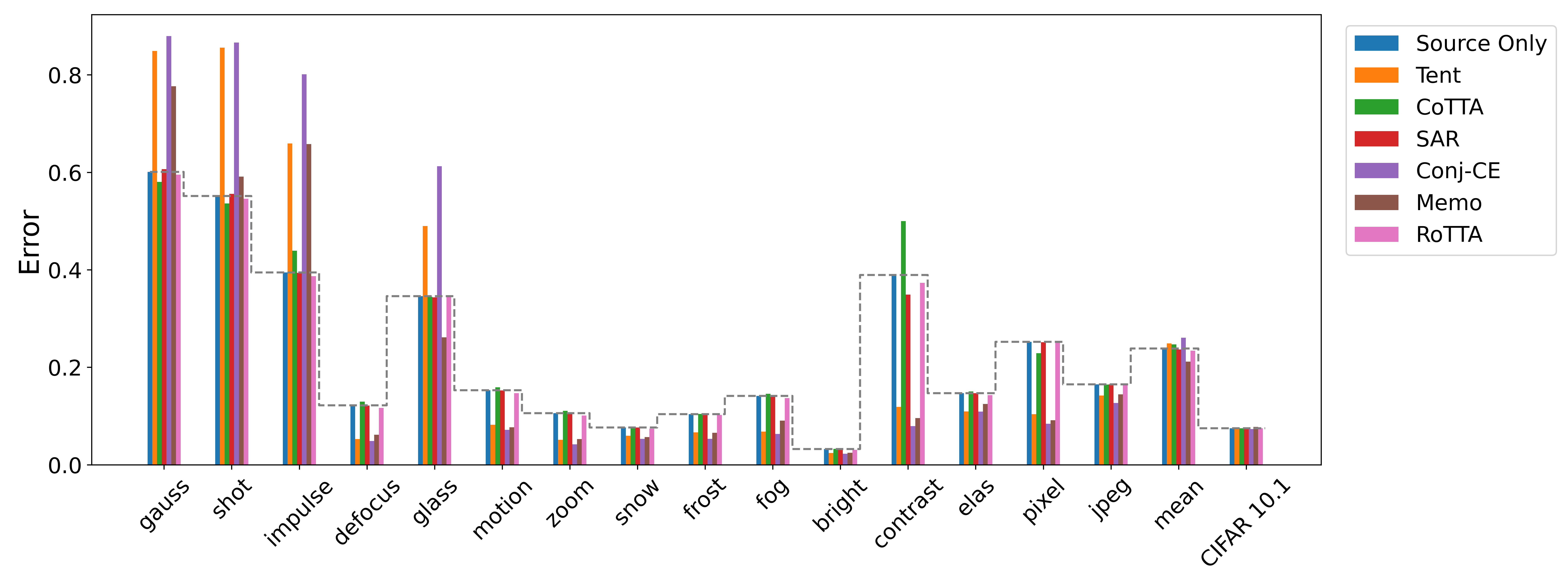
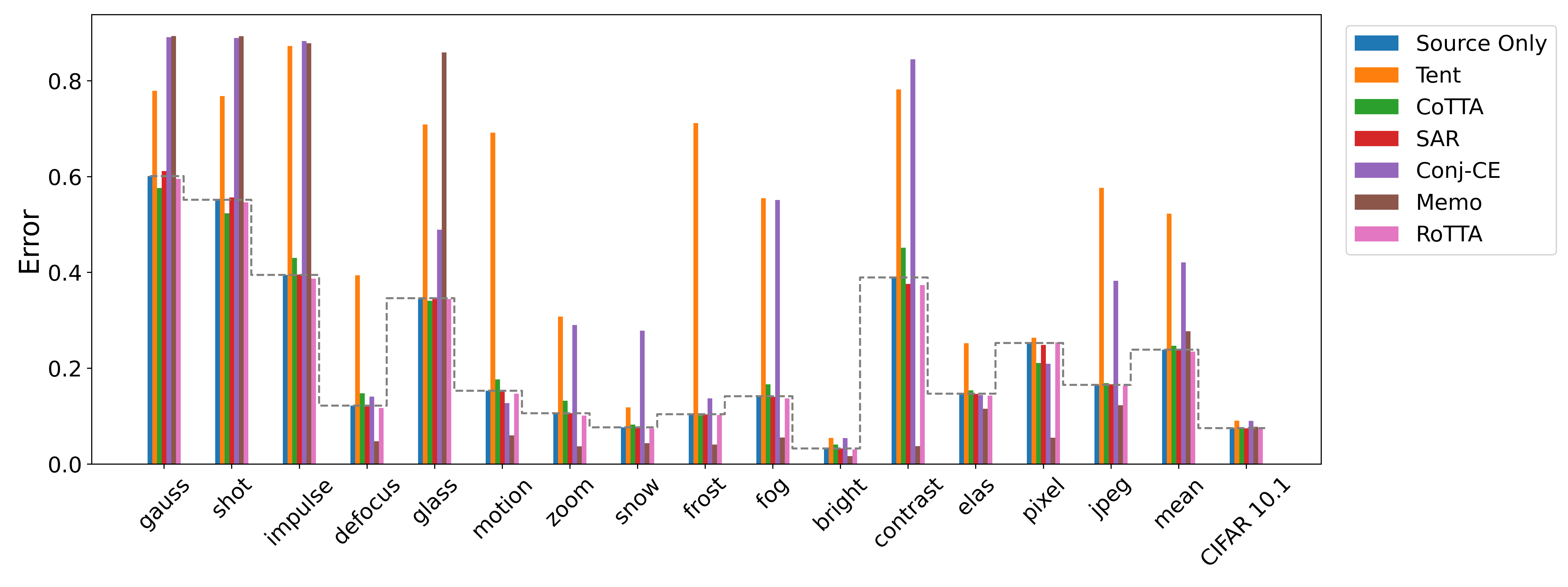
Figure 8: Comparison of the OTTA performance on the CIFAR-10-C (at severity level $5$) and CIFAR-10.1 datasets. The upper and bottom plots show the experiments conducted with batch size $16$ and $1$ based on the LayerNorm updating strategy, respectively.

Component substitution. To successfully adapt core methods for use with the Vision Transformer (ViT), we have developed a series of strategies:

• Switch to LayerNorm: In light of the absence of BatchNorm layer in ViT, we substitute all BatchNorm updates with LayerNorm updates.

• Disregard BatchNorm mixup: Removing statistic mixup strategy originally designed for BatchNorm-based methods as LayerNorm is designed to normalize each data point independently.

• Sample Embedding Changes: For OTTA methods that rely on feature representations, an effective solution is to use the class embedding (i.e., the first dimension of the ViT feature) as the image feature.

• Pruning Incompatible Components: Any elements incongruent with the ViT framework should be identified and removed.

These strategies lay the foundation for integrating core OTTA methods with the Vision Transformer, thereby broadening their application to this advanced model architecture. It’s important to note that these solutions are not exclusively limited to the OTTA methods. Rather, they can be viewed as a broader set of guidelines that can be applied where there is a need for upgrading to a new generation of backbone architectures.

Baselines: We carefully select seven methods to examine the adaptability of OTTA methods thoroughly. They include:

1. Tent: A fundamental OTTA method rooted in BatchNorm updates. To reproduce it on ViTs, we replace its BatchNorm updates with a LayerNorm updating strategy.

2. CoTTA employs the mean-teacher model, parameter reset, and selective augmentation strategy. While it necessitates updating the entire student network, we further assess the LayerNorm updating strategy on its student model. We also deconstruct its parameter reset strategy, resulting in four variants: parameter reset with LayerNorm updating (CoTTA-LN), parameter reset with full network updating (CoTTA-ALL), updating LayerNorm without parameter reset (CoTTA^∗-LN), and full network updating without parameter reset (CoTTA^∗-ALL).

3. SAR follows the same strategy as Tent while using sharpness-aware minimization for optimization.

4. Conj-PL: As the source model optimized by cross-entropy loss, it is similar to Tent but allows the model to interact with the data twice: once for updating LayerNorm and another for prediction.

5. MEMO: Two versions of MEMO are considered: full model updating and LayerNorm updating. We remove all data normalizations from its augmentation set to maintain consistency and prevent unexpected performance variations.

6. RoTTA: Due to the architecture limitation from ViTs, we exclude the RBN module in RoTTA. As LayerNorm in ViT is designed to handle data at the sample level, the RBN module is inapplicable.

7. TAST: We use the first dimension’s class embedding as the feature representation to suit ViT architecture.

Despite the large OTTA method pool, thoroughly evaluating this selected subset could yield valuable insights commensurate with our expectations. In the empirical study, we address the following key research questions:

4.2 Is OTTA still working with ViT?

To assess the efficacy of selected methods, we compare them against the source-only (i.e., direct inference) baseline. We discuss the experimental result for each dataset in the subsequent sections.

4.2.1 On CIFAR-10-C and CIFAR-10.1 Benchmarks

We evaluate the CIFAR-10-C and CIFAR-10.1 datasets with batch sizes $1$ and $16$ and show the result in Fig. 8. To clearly understand the pattern of predictions, we discuss our observations in three aspects: 1) variation in corruption types, 2) variation in batch sizes, and 3) variation in adaptation strategies.

Corruption Type. As depicted in Fig. 8 and Fig. 15, a notable observation is that most methods experience high error rates with noise corruptions, irrespective of their batch size. However, these methods exhibit reasonable performance for some other types of corruption. This difference may be attributed to the random and unpredictable nature of noise corruptions, as opposed to more structured types like snow, zoom, or brightness, which are potentially more comprehensible for online adaptation.

Furthermore, adapting to noise corruption poses a significant challenge for confidence optimization-based methods (Sec. 3.1.3), regardless of the batch size. This difficulty can be linked to the substantial domain gap and the unpredictable nature of noise patterns discussed earlier. Although these strategies aim to increase the model’s confidence, they are not equipped to directly correct erroneous predictions.

Batch Size. Variations in batch size do not significantly alter the mean error, with notable exceptions for Tent, Conj-CE, and MEMO. As observed in Sec. 4.4, we conclude that for purely optimization-based methods, a larger batch size can stabilize loss optimization, thereby benefiting adaptation. However, incorporating consideration of prediction reliability can substantially mitigate the constraints imposed by smaller batch sizes, as evidenced in methods like CoTTA, TAST, and SAR. A similar pattern is observed in CIFAR-10.1, where two entropy-based methods (Tent and Conj-CE) exhibit limitations at small batch sizes.

Adaptation Strategy. SAR and RoTTA demonstrate stable performance regardless of domain or batch size variations. The memory bank in RoTTA contributes to maintaining global information, rendering it more batch-agnostic. From a different angle, SAR achieves flat minima, which ensures model optimization for stability and prevents biased learning during adaptation. MEMO also displays impressive performance in certain domains, even with batch sizes as small as $1$.

4.2.2 On CIFAR-100-C Benchmark

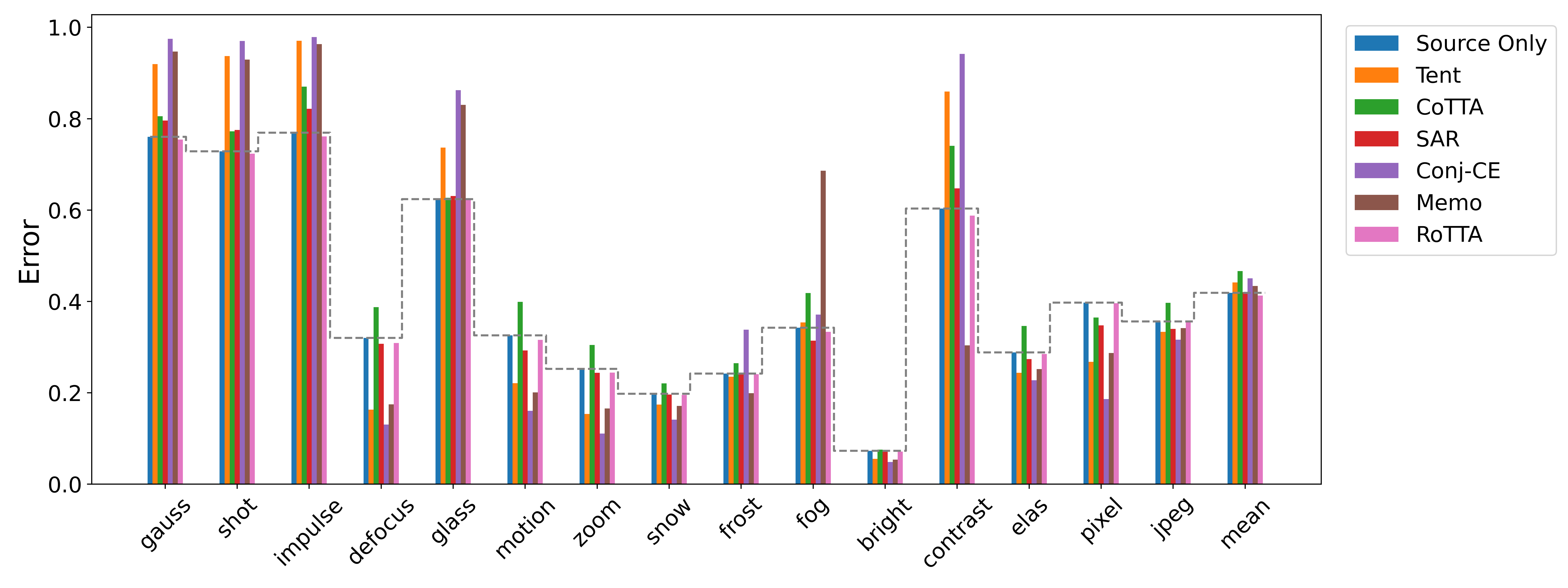
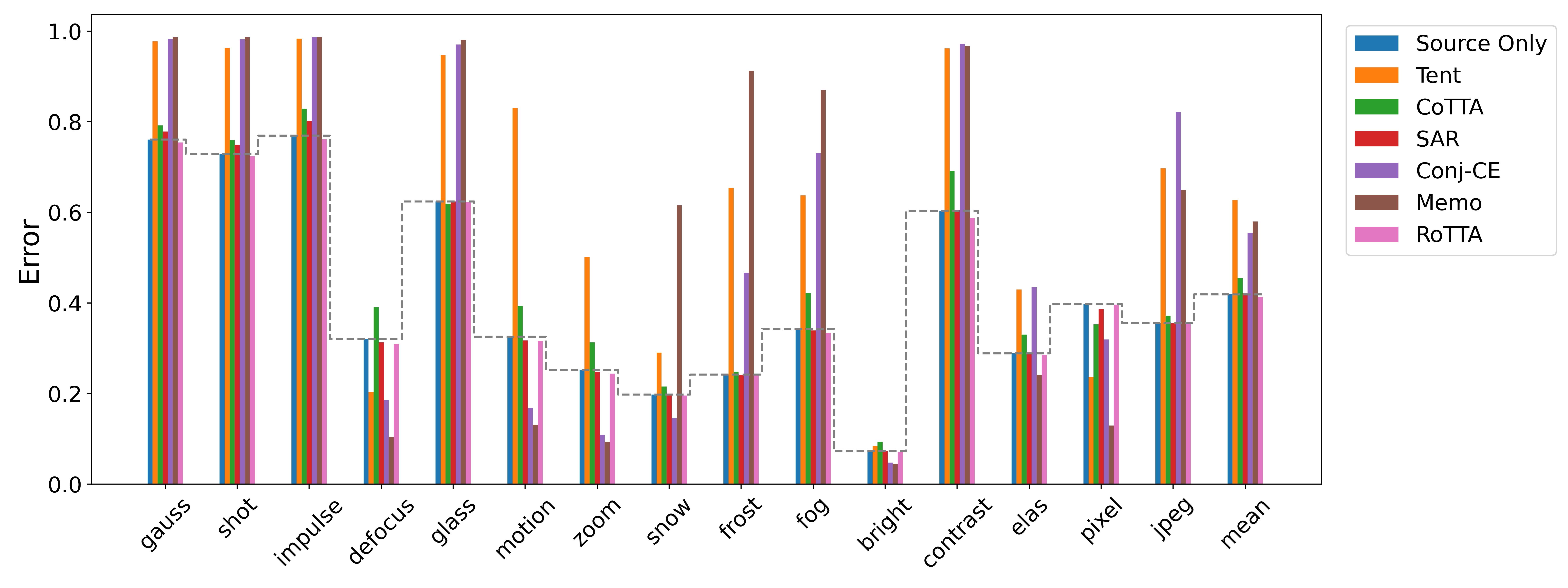
Figure 9: Comparison of the OTTA performance on the CIFAR-100-C severity level $5$. The upper and bottom plots show the experiments conducted with batch size $16$ and $1$ based on the LayerNorm updating strategy, respectively.

The performance on the CIFAR-100-C dataset exhibits a trend similar to that observed in the CIFAR-10-C dataset. To ensure a concise and focused discussion, we will explore specific adaptation strategies only when their performance patterns distinctly differ from those of the CIFAR-100-C dataset.

A notable observation is the comparatively less robust performance on CIFAR-100-C, especially when using a batch size of $16$. This decrease in performance is likely due to the greater complexity and variety in the CIFAR-100-C dataset, which includes a more extensive range of classes.

Adaptation Strategy. CoTTA demonstrates a noticeable decrease in effectiveness across most types of corruption, particularly with a batch size of $16$. This performance reduction can be partly attributed to the significant number of classes, for instance, comparing $10$ in CIFAR-10-C to $100$ in CIFAR-100-C. Additionally, the stochastic parameter reset might lead to the loss of newly acquired knowledge about these varied domains. Similarly, SAR begins to exhibit limitations, especially in the presence of noise distortions such as Gaussian, shot, and impulse noise.

An interesting observation is the performance degradation in the contrast corruption domain. Here, RoTTA stands out as the only method that consistently outperforms direct inference, irrespective of batch size. This underscores the importance of effectively preserving valuable sample information, particularly for tackling batch-sensitive and challenging adaptation tasks. A similar trend is observable in Fig. 10.

4.2.3 On Imagenet-C Benchmark

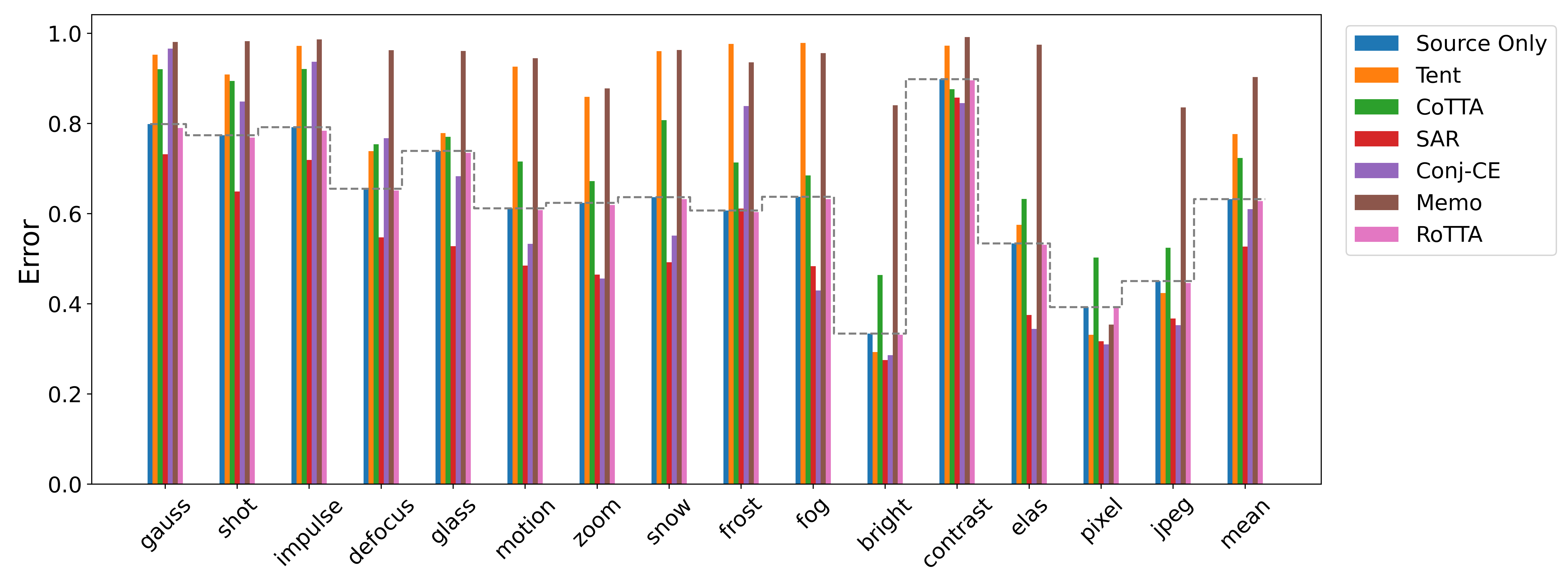
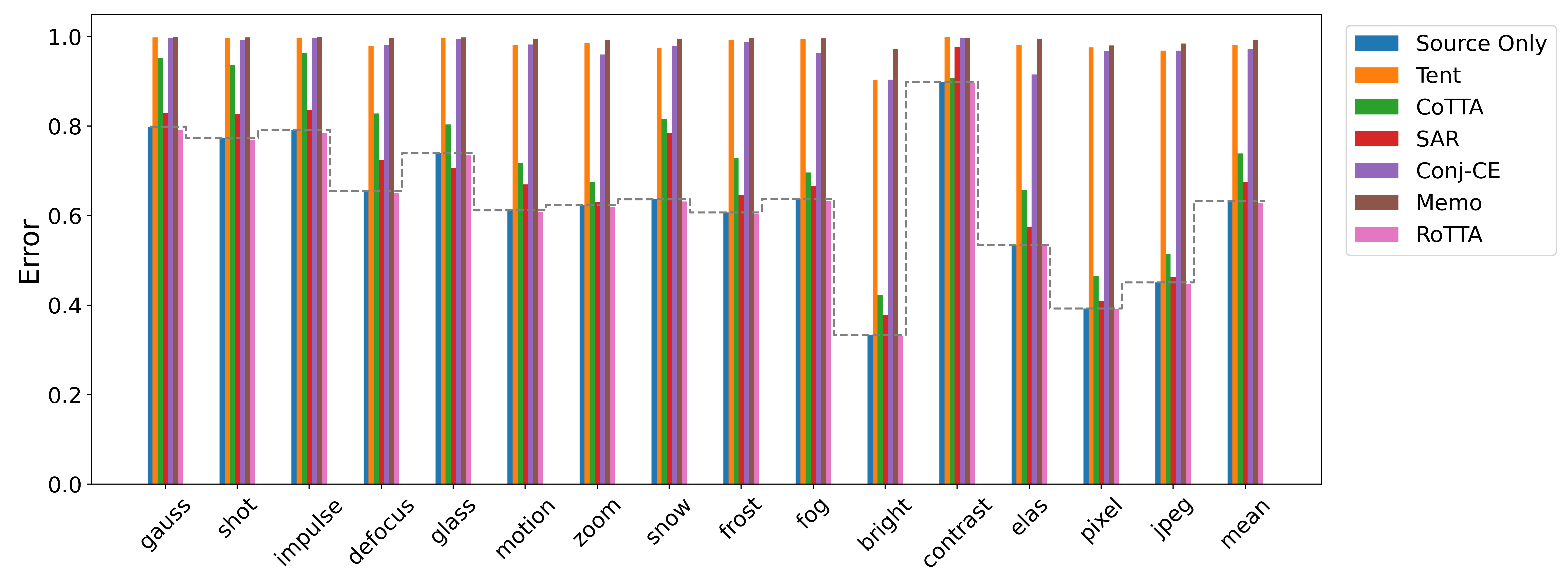
Figure 10: Comparison of the OTTA performance on the ImageNet-C severity level $5$. The upper and bottom plots show the experiments conducted with batch size $16$ and $1$ based on the LayerNorm updating strategy, respectively

Adaptation Strategy. For the ImageNet-C dataset depicted in Fig. 10, when the batch size is set to 16, SAR, Conj-CE, and RoTTA outperform the source-only model in terms of mean error. In contrast, Tent, MEMO, and CoTTA demonstrate significantly poor results. The error rate within each domain exhibits a similar trend. Notably, Conj-CE, which conducts an additional inference for each batch for final prediction, markedly surpasses Tent across most domains and in mean error. This suggests a significant inter-batch distribution shift in ImageNet-C, such as style or class differences, indicating that strategies based on optimizing the current batch for predicting the next batch are less effective. Additionally, MEMO faces challenges in scenarios characterized by complex label sets and significant data diversity. The parameter reset in CoTTA might also adversely affect the model’s discriminative capability, especially in complex environments.

When the batch size is reduced to 1, only RoTTA maintains its performance level, implying that typical unsupervised loss functions may be inadequate for complex adaptation tasks. Concurrently, preserving valuable data can significantly reduce the performance disparity caused by domain shifts.

Batch Size. Compared to CIFAR-10-C and CIFAR-100-C, ImageNet-C experiences more pronounced performance degradation, particularly when the batch size is reduced to 1. This observation, combined with our analysis of adaptation strategies, suggests that datasets with higher complexity and difficulty are more sensitive to changes in batch size.

Corruption Type. Relative to CIFAR-10-C and CIFAR-100-C datasets (as shown in Fig. 8 and Fig. 9), a distinctive feature of the ImageNet-C dataset is the narrower performance gap across various types of corruption. This implies that datasets with fewer classes are likely to show greater performance variability in response to different corruptions. For ImageNet-C, encompassing 1,000 classes, we observe consistently poor performance across all corruption domains, likely due to substantial inter-batch class differences, which hinder effective learning.

4.2.4 On CIFAR-10-Warehouse Benchmark

We assess OTTA techniques on the newly introduced CIFAR-10-Warehouse dataset, which shares the same label set as CIFAR-10-C. For our evaluation, we selected two representative domains within CIFAR-10-Warehouse. These domains were specifically chosen to gauge the performance of OTTA methods under two distinct distribution shifts: the real-world shift and the diffusion synthesis shift. The Google split consists of images sourced from the Google search engine. This subset serves as a critical benchmark for evaluating the capability of contemporary OTTA methods in managing real-world distribution shifts. We assess OTTA performance across its 12 subdomains labeled G-01 to G-12. Each subdomain represents images predominated by different main colors, providing a diverse range of visual scenarios to test the adaptability and effectiveness of OTTA methods under real-world conditions.

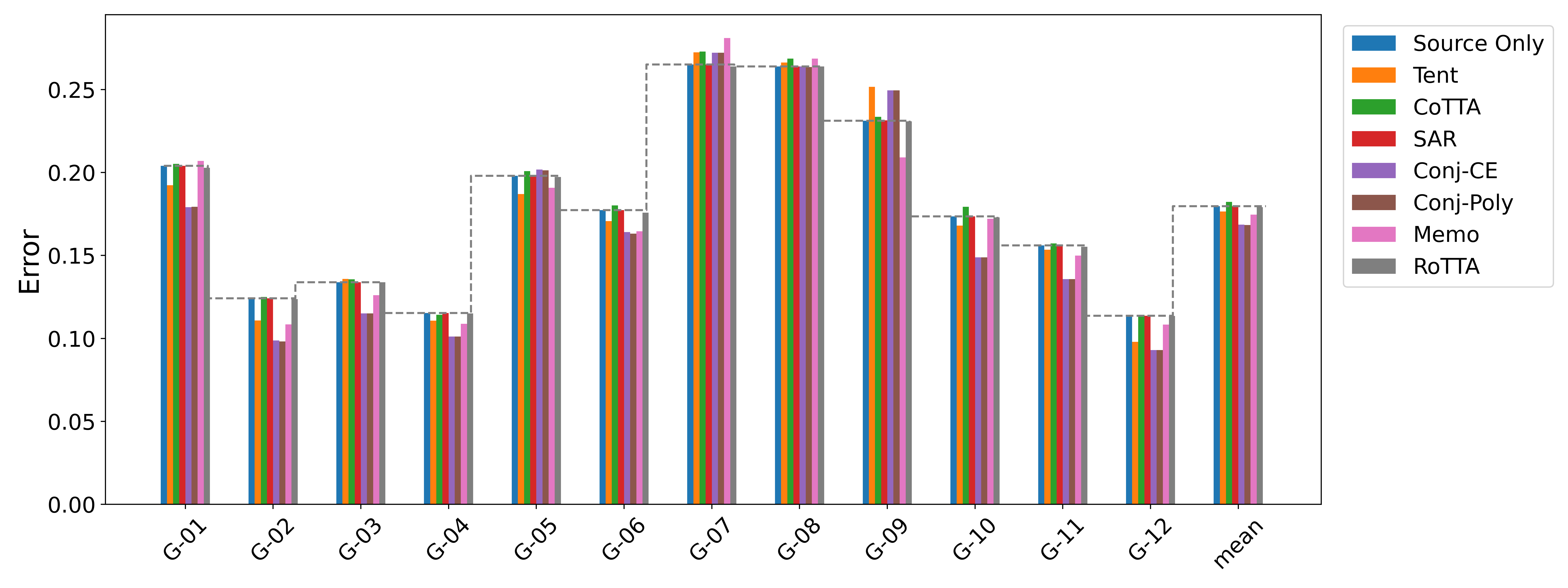
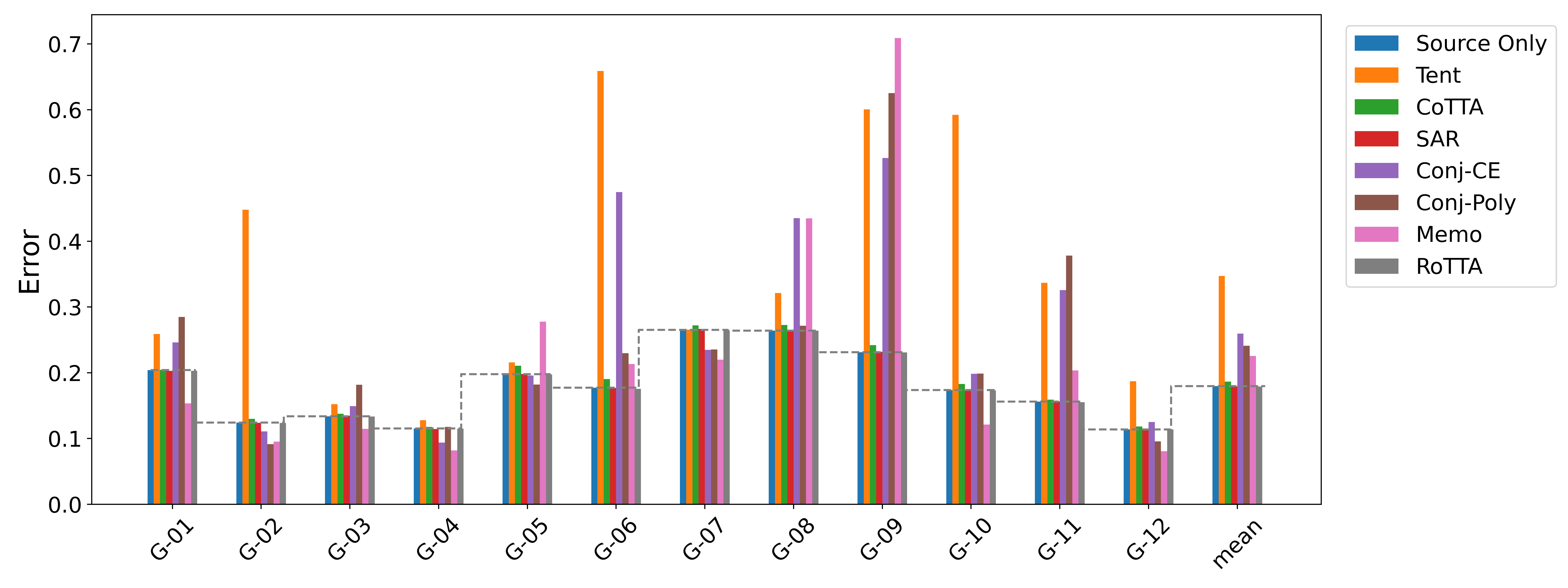
Figure 11: Comparison of the OTTA performance on the Google split of CIFAR-10-Warehouse. The upper and bottom plots show the experiments conducted with batch size $16$ and $1$ based on the LayerNorm updating strategy.

Batch Size. Regarding the batch size differences depicted in Fig. 11, we observe that when the batch size is $16$, most OTTA methods match or surpass the performance of direct inference. This outcome suggests that the current OTTA methods are generally effective. Additionally, the performance of most OTTA methods remains stable when the batch size is reduced to $1$. However, methods such as Tent and Conj-CE exhibit performance degradation in most domains. This may be attributed to the instability of optimization for single-sample batches, especially in Tent, which focuses solely on optimizing entropy.

Adaptation Strategy. RoTTA and SAR demonstrate exceptional stability regardless of batch sizes. This stability is achieved by preserving high-quality data information in RoTTA and seeking flat minima in its optimization in SAR. We compare Conj-CE with Conj-Poly, where Conj-Poly refers to the adaptation strategy when the source pre-training loss is poly loss (Leng et al, 2022). In our experiment, we modified the adaptation strategy without altering the source pre-training loss to observe performance differences. Interestingly, even when the batch size was set to 1, and the source pre-trained loss was cross-entropy loss (where Conj-Poly would not be the presumed optimal choice), Conj-Poly still managed to outperform Conj-CE in terms of mean error. This finding challenges the conclusions drawn in the original Conj-PL paper, suggesting that Conj-Poly might be more effective than initially thought, even when not aligned with the source pre-training loss.

Diffusion split. We evaluate OTTA methods within the diffusion subdomain.

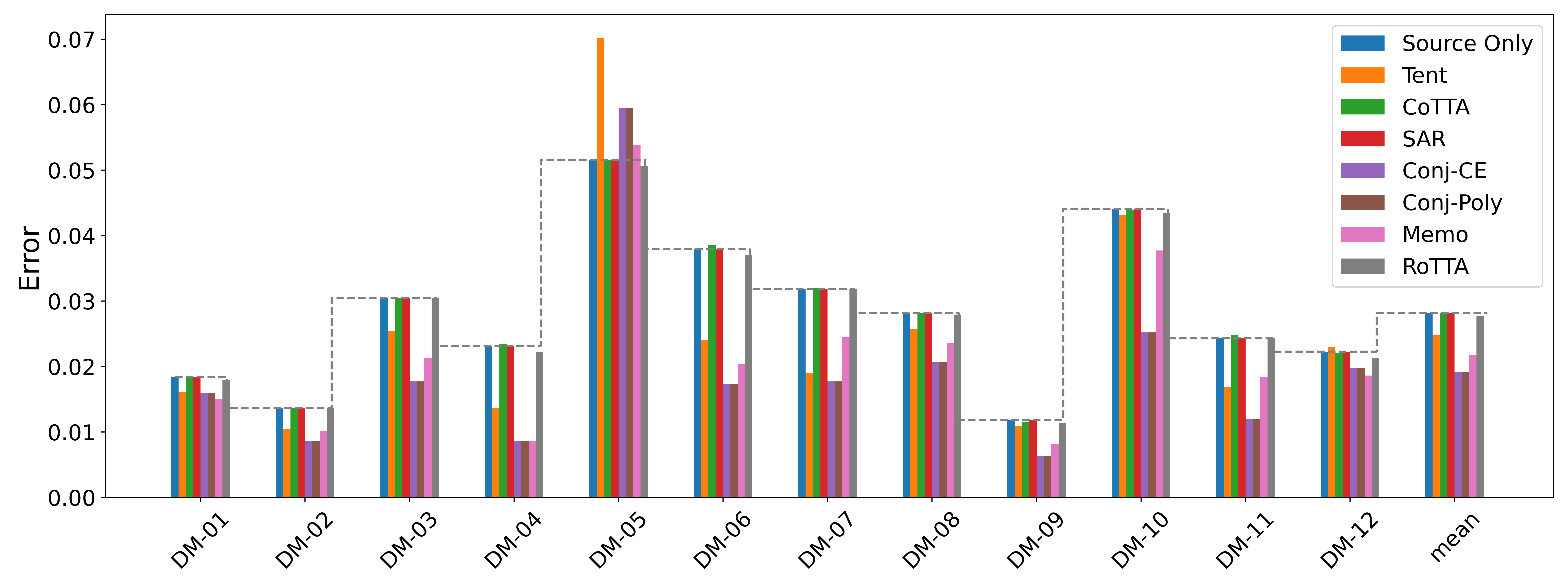
Figure 12: Comparison of the OTTA performance on the diffusion split of CIFAR-10-Warehouse. All the experiments are conducted with batch size $16$ based on the LayerNorm updating strategy. The dotted line indicates the baseline performance without any adaptation.

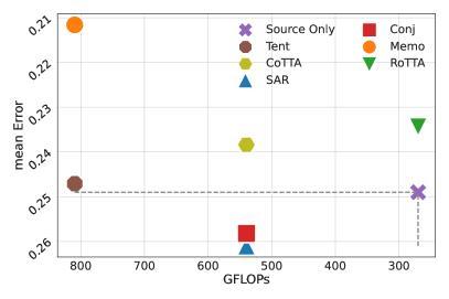
(a) Batch Size=16

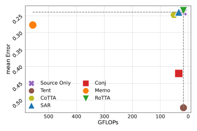
(b) Batch Size=1

Figure 13: Mean error vs Giga Floating Point Operations Per Second (GFLOPs). All experiments are conducted on a severity level of $5$. We plot their correlation under batch size $16$ and $1$ settings for the CIFAR-10-C dataset.

Subdomain Type. The results presented in Fig. 12 exhibit a consistent trend across 12 subdomains, with the exception of DM-$05$. In DM-$05$, confidence optimization methods perform less effectively compared to direct inference. This can be attributed to the substantial domain shift leading to distorted data interpretation. Relying solely on optimization in these methods may exacerbate model biases, especially due to prediction inaccuracy. In contrast, these methods excel in other domains, indicating the varying domain gaps across each diffusion-based subdomain.

Adaptation Strategy. Another noteworthy observation is the stable performance of CoTTA, SAR, and RoTTA. By employing sharpness-aware minimization, SAR enables the model to reach a region in the optimization landscape that is less sensitive to data variations, resulting in stable predictions. CoTTA’s parameter reset strategy effectively mitigates biased adaptation, allowing for partial knowledge restoration from the source domain, contributing to its consistent performance, even in the challenging DM-$05$ subdomain. Lastly, RoTTA, utilizing an informative memory bank, achieves commendable performance across the subdomains.

Conclusion. From our extensive experiments, most OTTA methods display similar behavioral patterns across various datasets. This consistency underscores the potential of contemporary OTTA techniques in effectively managing diverse domain shifts. Particularly noteworthy are RoTTA and SAR, highlighting the significance of optimization insensitivity and information preservation.

4.3 Is OTTA efficient?

To evaluate the performance of OTTA algorithms, particularly under hardware constraints, we utilize GFLOPs as a metric, as illustrated in Fig. 13. Lower GFLOPs and mean error is preferable. Our observation shows that MEMO achieves high performance but incurs higher computational costs. In contrast, RoTTA successfully balances low error rates with efficient updates. This also suggests that reducing the batch size could be beneficial in achieving a balance between performance and computational efficiency.

Figure 14: Impact of varying batch sizes on CIFAR-10.1, CIFAR-10-Warehouse, CIFAR-100-C, ImageNet-C. The base model is Tent optimized on LayerNorm.

4.4 Is OTTA sensitive to Hyperparameter Selection?

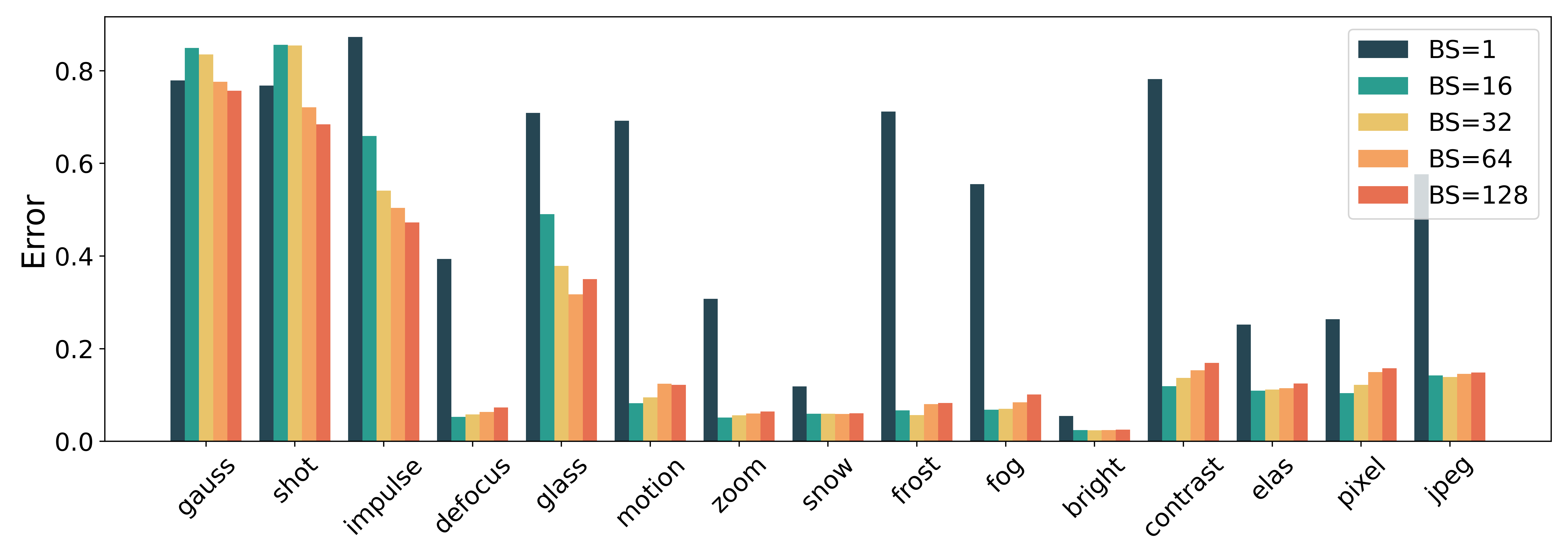
Figure 15: Impact of varying batch sizes on CIFAR-10-C severity level $5$. The base model is Tent optimized on LayerNorm.

Batch Size Matters, but only to an extent. Fig. 15 examines the impact of different batch sizes on Tent’s performance in the CIFAR-10-C dataset. It reveals that performance significantly varies with batch sizes from $1$ to $16$ across most corruptions. However, this variability diminishes with larger batch sizes ($16$ to $128$), indicating a reduced influence of LayerNorm updating on batch size, in contrast to traditional BatchNorm settings. This pattern is consistent across other datasets, as depicted in Fig. 14. Nevertheless, batch size remains crucial for stabilizing the optimization process. For example, a batch size of $16$ outperforms a batch size of $1$ in confidence optimization methods in the Google split of the CIFAR-10-Warehouse dataset. However, Larger batch sizes are essential for complex datasets like CIFAR-100-C and ImageNet-C, where direct inference struggles, emphasizing the need to tailor batch sizes to the data complexity. Additionally, Fig. 15 suggests that increasing batch sizes is not effective against challenging corruptions, such as Gaussian and Shot noise. This highlights the necessity for more advanced adaptation strategies beyond mere batch size adjustments in complex learning scenarios.

Table 2: The Comparison of model update strategies across five benchmarks: Layernorm only v.s. full model. ^∗ indicates the variant of CoTTA with no parameter reset mechanism.

Method	CIFAR-10-C			CIFAR-10.1			CIFAR-100-C			ImageNet-C			CIFAR-Warehouse
	LN	ALL	$\Delta$ Err	LN	ALL	$\Delta$ Err	LN	ALL	$\Delta$ Err	LN	ALL	$\Delta$ Err	LN	ALL	$\Delta$ Err
CoTTA	0.2471	0.5247	-52.91%	0.0750	0.1155	-35.06%	0.4663	0.6442	-27.62%	0.7237	0.8516	-15.02%	0.1823	0.2804	-34.99%
CoTTA$*$	0.2468	0.7708	-67.98%	0.0750	0.1640	-54.27%	0.4682	0.8961	-47.75%	0.7229	0.9054	-20.16%	0.1820	0.5463	-66.68%
MEMO	0.2116	0.8999	-76.49%	0.0780	0.9000	-91.33%	0.4338	0.9900	-56.18%	0.9032	0.9995	-96.35%	0.1746	0.8955	-80.50%

Optimization Layer Matters! To assess the critical role of LayerNorm, we compare LayerNorm-based optimization with full model optimization, as summarized in Table. 2. This ablation study primarily focused on CoTTA and MEMO, evaluating the impact of optimizing LayerNorm alone. A notable observation is, for all methods, LayerNorm update plays an important role in gaining high performance, underscoring its effectiveness in boosting model performance by avoiding significant forgetting of the source knowledge.

5 Future Directions

Our initial evaluations of the Vision Transformer revealed that many Online Test-Time Adaptation methods are not fully optimized for this architecture, resulting in suboptimal outcomes. Based on these findings, we propose several key attributes for an ideal OTTA approach, suitable for future research and tailored to advanced architectures like ViT:

• Refining OTTA in Realistic Settings: Future OTTA methods should undergo testing in realistic environments, employing advanced architectures, practical testbeds, and reasonable batch sizes. This approach aims to gain deeper and more relevant insights.

• Addressing Multimodal Challenges and Exploring Prompting Techniques: With the evolution towards foundation models like CLIP (Radford et al, 2021), OTTA is confronted with new challenges. These models may face shifts across various modalities, necessitating innovative OTTA strategies that extend beyond reliance on images alone. Exploring prompt-based methods could offer significant breakthroughs in OTTA.

• Hot-swappable OTTA: Keeping pace with the rapid evolution of backbone architectures is crucial. Future OTTA methods should focus on adaptability and generalizability to seamlessly integrate with evolving architectures.

• Stable and Robust Optimization for OTTA: Stability and robustness in optimization remain paramount. Given that larger batch sizes demonstrate limited effectiveness in ViT, future research should investigate more universal optimization improvements. Such advancements aim to consistently enhance model performance, independent of external factors like batch size.

6 Conclusion

In this survey, we thoroughly examine Online Test-Time Adaptation (OTTA), detailing existing methods, relevant datasets, benchmarks for evaluation, and their implementations. Comprehensive experiments are conducted to evaluate the effectiveness and efficiency of current OTTA methods when applied to vision transformers. Our observations indicate that noise-synthesized domain shifts often present more significant challenges compared to other types of shifts, such as those encountered in real-world scenarios or diffusion environments. Additionally, the presence of a large number of classes in a dataset can lead to noticeable discrepancies between batches, potentially impacting OTTA models’ ability to retain consistent knowledge. This may result in learning difficulties and an increased risk of severe forgetting. To address these challenges, we find that updating the normalization layer with a memory bank or optimization flatness, combined with proper batch size selection, can effectively stabilize the adaptation process and mitigate forgetting. We hope this survey will serve as a foundational reference, providing valuable insights for researchers and practitioners keen to explore the dynamic field of OTTA.

Data Availability Statement: The data that support the findings of this study are openly available as summarized in Table 1. This open-soured repository includes all the implementation code and experimental configurations of this work.

Table 3: The summary of existing OTTA published in the top-tier conferences before Nov-2023.

Year	Method	Model-based			Data-based		Optimization-based
		add.	subst.	prompt	mem.	aug.	loss.	pl.	t-s.	norm.
2021	Tent (Wang et al, 2021a)						✓			✓
2021	MixNorm (Hu et al, 2021)		✓							✓
2021	PAD (Wu et al, 2021)		✓			✓		✓
2021	TTPR (Sivaprasad et al, 2021)					✓	✓
2021	Core (You et al, 2021)									✓
2021	SLR (Mummadi et al, 2021)	✓					✓			✓
2021	T3A (Iwasawa and Matsuo, 2021)		✓		✓
2022	NOTE (Gong et al, 2022)				✓					✓
2022	EATA (Niu et al, 2022)									✓
2022	CoTTA (Wang et al, 2022a)					✓			✓
2022	Conj-PL (Goyal et al, 2022)						✓	✓		✓
2022	GpreBN (Yang et al, 2022)		✓							✓
2022	CFA (Kojima et al, 2022)									✓
2022	DUA (Mirza et al, 2022)		✓			✓				✓
2022	MEMO (Zhang et al, 2022)					✓	✓			✓
2022	AdaContrast (Chen et al, 2022)				✓	✓	✓	✓
2022	TPT (Shu et al, 2022)			✓
2022	DePT (Gao et al, 2022)			✓
2023	DN (Gan et al, 2023)			✓
2023	TAST (Jang et al, 2023)	✓	✓		✓					✓
2023	MECTA (Hong et al, 2023)		✓							✓
2023	DELTA (Zhao et al, 2023a)		✓							✓
2023	TeSLA (Tomar et al, 2023)				✓	✓	✓		✓
2023	RoTTA (Yuan et al, 2023b)		✓		✓	✓			✓	✓
2023	EcoTTA (Song et al, 2023)	✓								✓
2023	TIPI (Nguyen et al, 2023)					✓				✓
2023	TSD (Wang et al, 2023)		✓		✓		✓
2023	SAR (Niu et al, 2023)						✓			✓
2023	ECL (Han et al, 2023)				✓			✓
2023	REALM (Seto et al, 2023)						✓			✓
2023	TTC (Lin et al, 2023)					✓	✓
2023	SoTTA (Gong et al, 2023)				✓		✓			✓
2023	ViDA (Liu et al, 2023b)	✓				✓			✓
2023	ERSK (Niloy et al, 2023)		✓							✓

Appendix A Appendix

This appendix offers tables about the categorization of OTTA methods and experiments conducted on the seven selected methods across the chosen datasets.

• Table 3: The summary of existing OTTA methods.

• Table 4: Experiments on the CIFAR-10 $\rightarrow$ CIFAR-10-C task.

• Table 5: Experiments on the CIFAR-100 $\rightarrow$ CIFAR-100-C task.

• Table 6: Experiments on the ImageNet-1k $\rightarrow$ ImageNet-C task.

• Table 7: Experiments on the CIFAR-10 $\rightarrow$ CIFAR-10-Warehouse task.

Table 4: Classification error rate ($\%$) and GFLOPs for the standard CIFAR-10 $\rightarrow$ CIFAR-10-C online test-time adaptation task. Results are evaluated on ViT-base-patch16-224 with the largest corruption severity level 5.

Method	Glass	Fog	Defoc.	Impul.	Contr.	Gauss.	Elastic.	Zoom	Pixel	Frost	Snow	JPEG	Motion	Shot	Brit.	Mean	GFLOPs
Source Only	34.60	14.14	12.20	39.47	38.95	60.12	14.70	10.61	25.26	10.39	7.67	16.51	15.30	55.17	3.26	23.89	269.81
Batch size = 16
Tent	49.02	6.81	5.29	65.93	11.91	84.93	10.96	5.12	10.41	6.68	5.96	14.21	8.25	85.60	2.43	24.90	269.81
CoTTA-LN	34.50	14.57	12.97	43.96	50.01	58.04	15.05	11.09	22.92	10.43	7.75	16.46	15.92	53.65	3.27	24.71	809.42
CoTTA-ALL	71.68	51.28	38.25	82.60	79.30	85.57	31.22	16.51	39.95	36.75	37.38	37.37	81.00	88.54	9.72	52.47	809.42
CoTTA$*$-LN	34.58	14.60	13.02	43.71	49.71	58.00	15.03	11.09	22.96	10.45	7.67	16.53	15.93	53.68	3.24	24.68	809.42
CoTTA$*$-ALL	77.17	78.07	70.48	85.98	81.41	86.57	74.54	66.80	68.95	78.34	72.30	79.23	79.62	88.83	67.91	77.08	809.42
SAR	34.39	14.13	12.18	39.38	34.92	60.67	14.70	10.61	25.17	10.39	7.67	16.51	15.28	55.59	3.26	23.66	539.61
Conj-CE	61.26	6.36	4.89	80.12	7.94	87.96	10.92	4.20	8.43	5.32	5.33	12.71	7.18	86.63	2.27	26.10	539.61
MEMO-LN	26.15	9.08	6.17	65.80	9.58	77.68	12.48	5.29	9.14	6.59	5.71	14.45	7.71	59.15	2.49	21.16	809.42
RoTTA-LN	34.47	13.72	11.70	38.72	37.35	59.55	14.29	10.14	25.38	10.25	7.42	16.31	14.70	54.59	3.07	23.44	269.81
TAST	81.25	88.58	81.23	83.31	87.40	84.15	78.54	79.59	78.03	81.12	79.51	78.92	81.93	83.55	75.00	81.47	268.45
Batch size = 1
Tent	70.90	55.50	39.38	87.28	78.20	77.92	25.22	30.77	26.38	71.19	11.85	57.65	69.19	76.82	5.48	52.25	16.86
CoTTA-LN	34.09	16.63	14.79	43.05	45.14	57.63	15.39	13.23	21.11	10.15	8.25	16.88	17.68	52.36	4.07	24.70	50.59
CoTTA-ALL	87.81	89.90	86.13	89.17	88.82	89.55	84.91	87.77	86.30	87.42	89.17	88.67	89.06	89.22	81.65	87.70	50.59
CoTTA$*$-LN	35.88	18.35	16.96	46.27	47.31	58.21	17.49	15.12	20.95	10.78	9.60	18.15	19.72	52.15	4.83	26.12	50.59
CoTTA$*$-ALL	89.79	89.76	86.30	89.63	89.66	89.78	89.17	89.12	89.32	88.04	89.44	89.18	88.76	89.67	87.83	89.03	50.59
SAR	34.63	14.04	12.03	39.55	37.62	61.17	14.63	10.61	24.85	10.38	7.62	16.63	15.20	55.67	3.27	23.86	33.73
Conj-CE	48.90	55.11	14.09	88.28	84.49	89.11	14.39	29.01	20.95	13.70	27.84	38.25	12.71	88.95	5.43	42.08	33.73
MEMO-LN	85.91	5.55	4.77	87.84	3.76	89.33	11.54	3.70	5.52	4.08	4.36	12.28	6.01	89.32	1.65	27.71	556.48
RoTTA-LN	34.46	13.72	11.71	38.72	37.36	59.55	14.29	10.12	25.39	10.24	7.43	16.32	14.71	54.62	3.07	23.45	16.86
TAST	81.23	88.59	81.35	83.59	87.76	84.37	78.78	79.32	77.96	81.20	79.61	78.98	82.05	83.63	75.48	81.59	16.78

Table 5: Classification error rate ($\%$) for the standard CIFAR-100 $\rightarrow$ CIFAR-100-C online test-time adaptation task. Results are evaluated on ViT-base-patch16-224 with the largest corruption severity level 5.

Method	Glass	Fog	Defoc.	Impul.	Contr.	Gauss.	Elastic.	Zoom	Pixel	Frost	Snow	JPEG	Motion	Shot	Brit.	Mean
Source-Only	62.39	34.23	32.01	76.94	60.32	76.05	28.86	25.25	39.73	24.20	19.79	35.62	32.56	72.86	7.32	41.88
Batch size = 16
Tent	73.69	35.40	16.33	97.06	85.94	91.95	24.4	15.37	26.78	23.54	17.44	33.36	22.09	93.71	5.53	44.17
CoTTA-LN	62.68	41.84	38.77	87.01	74.04	80.53	34.62	30.46	36.46	26.47	22.08	39.70	39.89	77.25	7.58	46.63
CoTTA-ALL	68.75	79.77	45.56	98.58	97.81	94.80	65.83	53.62	38.73	37.63	24.49	67.40	86.00	94.18	13.19	64.42
CoTTA$*$-LN	63.12	42.25	39.1	87.11	73.93	80.57	34.94	30.71	36.75	26.3	22.42	39.79	40.22	77.47	7.60	46.82
CoTTA$*$-ALL	91.58	91.85	83.09	98.61	97.91	97.39	91.57	90.03	86.26	83.19	79.11	90.57	93.47	97.00	72.5	89.61
SAR	63.09	31.41	30.72	82.17	64.76	79.59	27.39	24.36	34.76	24.1	19.61	34.01	29.26	77.55	7.32	42.01
Conj-CE	86.24	37.12	13.06	97.87	94.18	97.49	22.73	11.07	18.64	33.83	14.13	31.64	16.06	97.03	4.86	45.06
MEMO-LN	83.03	68.62	17.49	96.33	30.39	94.71	25.19	16.58	28.71	19.93	17.13	34.18	20.07	92.96	5.38	43.38
RoTTA-LN	62.22	33.34	30.92	76.12	58.78	75.42	28.51	24.41	39.61	24.1	19.55	35.49	31.59	72.36	7.14	41.3
TAST	95.72	97.73	95.93	98.06	98.13	97.87	94.83	94.89	94.09	95.96	95.01	96.03	95.56	97.76	93.1	96.04
Batch size = 1
Tent	94.66	63.74	20.36	98.33	96.17	97.72	42.98	50.11	23.65	65.41	29.05	69.70	83.09	96.28	8.43	62.65
CoTTA-LN	61.94	42.16	39.05	82.87	69.13	79.16	33.02	31.30	35.29	24.84	21.57	37.19	39.32	75.95	9.32	45.47
CoTTA-ALL	96.95	93.78	95.34	98.9	97.82	98.86	92.47	93.33	96.36	95.66	98.42	95.79	96.81	98.68	98.04	96.48
CoTTA$*$-LN	66.87	46.04	42.94	85.11	71.35	82.93	39.81	35.38	38.61	30.09	27.39	45.03	44.50	79.71	11.59	49.82
CoTTA$*$-ALL	98.62	98.36	98.26	98.87	98.6	98.95	98.11	97.64	98.63	98.25	98.62	98.38	98.04	98.90	98.49	98.45
SAR	62.39	33.95	31.29	80.15	60.48	77.82	28.63	24.83	38.60	24.12	19.87	35.51	31.73	74.89	7.29	42.10
Conj-CE	97.07	73.10	18.54	98.67	97.21	98.25	43.5	10.9	31.95	46.68	14.56	82.12	16.89	98.18	4.75	55.49
MEMO-LN	98.08	86.99	10.42	98.69	96.71	98.64	24.14	9.35	12.94	91.24	61.54	64.93	13.12	98.63	4.45	57.99
RoTTA-LN	62.22	33.34	30.92	76.11	58.78	75.41	28.51	24.40	39.63	24.10	19.55	35.49	31.59	72.36	7.14	41.30
TAST	95.77	97.82	95.97	98.10	98.11	97.96	94.85	94.93	94.04	95.99	95.13	96.33	95.63	97.73	93.25	96.11

Table 6: Classification error rate ($\%$) for the standard ImageNet-1k $\rightarrow$ ImageNet-C online test-time adaptation task. Results are evaluated on ViT-base-patch16-224 with the largest corruption severity level 5.

ImageNet-C	Glass	Fog	Defoc.	Impul.	Contr.	Gauss.	Elastic.	Zoom	Pixel	Frost	Snow	JPEG	Motion	Shot	Brit.	Mean
Source-Only	73.92	63.76	65.54	79.18	89.84	79.88	53.38	62.42	39.26	60.70	63.66	45.06	61.20	77.38	33.38	63.24
Batch size = 16
Tent	77.86	97.88	73.88	97.24	97.28	95.28	57.54	85.92	33.12	97.64	96.06	42.40	92.60	90.88	29.30	77.66
CoTTA-ALL	73.72	94.82	92.80	99.14	92.94	99.06	78.06	84.14	79.40	88.92	96.70	54.48	86.58	98.10	58.48	85.16
CoTTA-LN	77.06	68.50	75.4	92.10	87.60	92.06	63.28	67.24	50.28	71.36	80.74	52.46	71.58	89.46	46.40	72.37
CoTTA$*$-ALL	90.30	95.84	95.08	99.28	95.24	99.12	87.9	88.2	90.20	94.84	97.50	68.04	95.82	98.68	62.08	90.54
CoTTA$*$-LN	77.26	68.6	75.32	91.58	87.08	92.28	63.3	67.18	50.72	70.74	80.64	52.02	71.48	89.72	46.46	72.29
SAR	52.78	48.34	54.74	71.92	85.74	73.18	37.54	46.48	31.70	61.14	49.24	36.74	48.48	64.92	27.52	52.70
Conj-CE	68.30	42.96	76.74	93.70	84.52	96.60	34.46	45.64	31.00	83.90	55.12	35.28	53.32	84.88	28.6	61.00
Conj-Poly	68.26	47.48	54.08	93.68	75.82	96.68	34.08	47.42	29.94	81.26	65.06	36.06	68.36	87.7	29.16	61.00
MEMO-LN	96.10	95.62	96.26	98.68	99.18	98.08	97.48	87.80	35.40	93.58	96.30	83.56	94.50	98.26	84.06	90.32
RoTTA-LN	73.50	63.24	65.14	78.40	89.58	79.02	53.10	61.94	39.12	60.34	63.24	44.62	60.80	76.88	33.12	62.80
TAST	99.76	99.64	99.74	99.68	99.90	99.64	99.46	99.30	99.12	99.46	99.32	98.78	99.58	99.36	98.44	99.41
Batch size = 1
Tent	99.66	99.46	97.90	99.64	99.84	99.80	98.16	98.60	97.56	99.28	97.46	96.90	98.18	99.66	90.34	98.16
CoTTA-ALL	99.24	99.64	99.06	99.54	99.78	99.80	97.94	99.20	97.48	98.08	99.20	98.60	99.46	99.02	94.82	98.72
CoTTA-LN	80.38	69.62	82.82	96.40	90.80	95.30	65.80	67.46	46.52	72.82	81.56	51.42	71.74	93.66	42.28	73.91
CoTTA$*$-ALL	99.62	99.70	99.54	99.60	99.82	99.80	98.82	99.48	99.30	99.28	99.58	99.20	99.60	99.64	98.70	99.45
CoTTA$*$-LN	82.84	72.14	84.56	94.98	92.66	94.66	66.16	70.64	48.88	78.10	83.78	51.62	76.08	91.92	45.12	75.61
SAR	70.58	66.64	72.40	83.60	97.76	82.96	57.54	62.98	41.02	64.54	78.52	46.34	66.96	82.72	37.78	67.49
Conj-CE	99.38	96.42	98.18	99.76	99.74	99.76	91.54	96.02	96.74	98.86	97.86	96.90	98.26	99.14	90.38	97.26
MEMO-LN	99.82	99.58	99.78	99.84	99.72	99.90	99.54	99.30	98.04	99.66	99.48	98.46	99.52	99.80	97.30	99.32
RoTTA-LN	73.46	63.26	65.10	78.40	89.58	79.04	53.14	61.94	39.12	60.36	63.18	44.64	60.86	76.88	33.12	62.81
TAST	99.76	99.68	99.70	99.66	99.88	99.64	99.42	99.26	99.18	99.46	99.32	98.74	99.60	99.38	98.42	99.41

Table 7: Classification error rate ($\%$) for the CIFAR-10 $\rightarrow$ CIFAR-10-Warehouse online test-time adaptation task. Results are evaluated on ViT-base-patch16-224 with the Google split and diffusion split.

Google	G-01	G-02	G-03	G-04	G-05	G-06	G-07	G-08	G-09	G-10	G-11	G-12	Mean
Source-Only	20.41	12.42	13.39	11.53	19.80	17.74	26.51	26.4	23.12	17.36	15.61	11.37	17.97
Batch size = 16
Tent	19.23	11.08	13.59	11.07	18.7	17.07	27.25	26.63	25.17	16.8	15.35	9.80	17.65
CoTTA-LN	20.52	12.50	13.56	11.43	20.09	18.02	27.29	26.87	23.36	17.93	15.73	11.43	18.23
CoTTA-ALL	22.28	21.89	29.76	10.55	22.47	20.96	40.86	44.11	41.56	26.07	31.80	24.21	28.04
CoTTA$*$-LN	20.55	12.48	13.54	11.47	20.04	17.93	27.25	26.71	23.30	17.81	15.88	11.41	18.20
CoTTA$*$-ALL	40.13	60.93	61.92	33.15	50.54	48.50	56.21	58.46	61.05	61.48	59.86	63.37	54.63
SAR	20.41	12.42	13.39	11.53	19.80	17.74	26.51	26.40	23.15	17.36	15.61	11.37	17.97
Conj-CE	17.91	9.87	11.51	10.11	20.18	16.41	27.22	26.40	24.96	14.89	13.57	9.30	16.86
MEMO-LN	20.70	10.84	12.61	10.88	19.08	16.46	28.11	26.87	20.91	17.21	14.99	10.83	17.46
MEMO-ALL	74.62	90.31	91.95	89.39	92.81	92.49	90.51	92.71	87.48	92.28	89.94	90.07	89.55
RoTTA-LN	20.29	12.37	13.39	11.51	19.73	17.58	26.40	26.40	23.09	17.30	15.52	11.35	17.91
TAST	66.74	71.80	62.10	76.22	79.94	80.28	84.20	76.02	77.67	83.63	83.02	76.23	76.49
Batch size = 1
Tent	25.90	44.81	15.22	12.77	21.57	65.91	26.55	32.14	60.05	59.22	33.68	18.70	34.71
CoTTA-LN	20.44	12.99	13.76	11.78	21.07	19.05	27.22	27.27	24.20	18.30	15.90	11.83	18.65
CoTTA-ALL	84.36	74.83	71.15	83.16	78.50	87.64	81.61	80.46	84.98	85.87	83.04	82.22	81.49
CoTTA$*$-LN	20.70	13.50	14.11	11.97	21.35	19.31	27.29	28.18	24.57	18.49	15.73	12.33	18.96
CoTTA$*$-ALL	86.81	85.35	86.21	87.08	88.44	87.41	72.75	90.88	84.03	89.93	85.44	85.36	85.81
SAR	20.29	12.40	13.46	11.45	19.82	17.70	26.66	26.24	23.17	17.30	15.64	11.33	17.95
Conj-CE	24.63	11.08	14.94	9.37	19.58	47.47	23.47	43.52	52.68	19.84	32.57	12.52	25.97
MEMO-LN	15.35	9.53	11.48	8.18	27.78	21.33	21.99	43.48	70.91	12.14	20.35	8.06	22.55
MEMO-ALL	74.62	90.96	91.95	89.39	92.81	92.49	97.44	92.75	87.48	92.28	89.94	90.07	90.18
RoTTA-LN	20.29	12.37	13.36	11.51	19.73	17.56	26.44	26.40	23.09	17.30	15.52	11.37	17.91
TAST	66.86	72.10	62.32	76.33	79.99	80.37	84.28	75.51	77.77	83.75	83.21	76.50	76.58
Diffusion	DM-01	DM-02	DM-03	DM-04	DM-05	DM-06	DM-07	DM-08	DM-09	DM-10	DM-11	DM-12	Mean
Source-Only	1.84	1.36	3.05	2.32	5.16	3.80	3.18	2.82	1.18	4.41	2.43	2.23	2.82
Batch size = 16
Tent	1.61	1.05	2.55	1.36	7.02	2.41	1.91	2.57	1.09	4.32	1.68	2.30	2.49
CoTTA-LN	1.84	1.36	3.05	2.34	5.16	3.86	3.21	2.82	1.16	4.39	2.48	2.21	2.82
CoTTA-ALL	13.80	15.07	9.46	10.41	44.77	17.86	21.18	13.93	1.43	44.20	2.73	20.25	17.92
SAR	1.84	1.36	3.05	2.32	5.16	3.80	3.18	2.82	1.18	4.41	2.43	2.23	2.82
Conj-CE	1.59	0.86	1.77	0.86	5.96	1.73	1.77	2.07	0.64	2.52	1.21	1.98	1.91
Conj-Poly	1.59	0.86	1.77	0.86	5.96	1.73	1.77	2.07	0.64	2.52	1.21	1.98	1.91
MEMO-LN	1.50	1.02	2.14	0.86	5.39	2.05	2.46	2.36	0.82	3.77	1.84	1.86	2.17
MEMO-ALL	90.91	90.91	90.91	90.91	90.91	90.89	90.91	90.89	90.91	90.89	90.66	90.91	90.88
RoTTA-LN	1.80	1.36	3.05	2.23	5.07	3.71	3.18	2.80	1.14	4.34	2.43	2.14	2.77
TAST	54.18	68.57	49.02	63.95	64.64	68.95	59.89	59.57	70.93	73.20	70.16	65.91	64.08

References

- Adachi et al (2023) Adachi K, Yamaguchi S, Kumagai A (2023) Covariance-aware feature alignment with pre-computed source statistics for test-time adaptation to multiple image corruptions. In: ICIP, IEEE, pp 800–804
- Ba et al (2016) Ba LJ, Kiros JR, Hinton GE (2016) Layer normalization. CoRR abs/1607.06450, 1607.06450
- Barron (2019) Barron JT (2019) A general and adaptive robust loss function. In: CVPR, Computer Vision Foundation / IEEE, pp 4331–4339
- Boudiaf et al (2022) Boudiaf M, Müller R, Ayed IB, Bertinetto L (2022) Parameter-free online test-time adaptation. In: CVPR, IEEE, pp 8334–8343
- Brahma and Rai (2023) Brahma D, Rai P (2023) A probabilistic framework for lifelong test-time adaptation. In: IEEE/CVF Conference on Computer Vision and Pattern Recognition, CVPR, IEEE, pp 3582–3591
- Carlucci et al (2017) Carlucci FM, Porzi L, Caputo B, Ricci E, Bulò SR (2017) Autodial: Automatic domain alignment layers. In: ICCV, IEEE Computer Society, pp 5077–5085
- Chakrabarty et al (2023) Chakrabarty G, Sreenivas M, Biswas S (2023) SATA: source anchoring and target alignment network for continual test time adaptation. CoRR abs/2304.10113, 2304.10113
- Chen et al (2022) Chen D, Wang D, Darrell T, Ebrahimi S (2022) Contrastive test-time adaptation. In: CVPR, IEEE, pp 295–305
- Chen et al (2009) Chen Y, Garcia EK, Gupta MR, Rahimi A, Cazzanti L (2009) Similarity-based classification: Concepts and algorithms. J Mach Learn Res 10:747–776
- Choi et al (2021) Choi M, Choi J, Baik S, Kim TH, Lee KM (2021) Test-time adaptation for video frame interpolation via meta-learning. IEEE Transactions on Pattern Analysis and Machine Intelligence 44(12):9615–9628
- Choi et al (2022) Choi S, Yang S, Choi S, Yun S (2022) Improving test-time adaptation via shift-agnostic weight regularization and nearest source prototypes. In: ECCV, Springer, Lecture Notes in Computer Science, vol 13693, pp 440–458
- Cogswell et al (2016) Cogswell M, Ahmed F, Girshick RB, Zitnick L, Batra D (2016) Reducing overfitting in deep networks by decorrelating representations. In: ICLR
- Ding et al (2022) Ding N, Xu Y, Tang Y, Xu C, Wang Y, Tao D (2022) Source-free domain adaptation via distribution estimation. In: CVPR, IEEE, pp 7202–7212
- Ding et al (2023) Ding Y, Liang J, Jiang B, Zheng A, He R (2023) Maps: A noise-robust progressive learning approach for source-free domain adaptive keypoint detection. arXiv preprint arXiv:230204589
- Döbler et al (2023) Döbler M, Marsden RA, Yang B (2023) Robust mean teacher for continual and gradual test-time adaptation. In: CVPR, IEEE, pp 7704–7714
- Dosovitskiy et al (2021) Dosovitskiy A, Beyer L, Kolesnikov A, Weissenborn D, Zhai X, Unterthiner T, Dehghani M, Minderer M, Heigold G, Gelly S, Uszkoreit J, Houlsby N (2021) An image is worth 16x16 words: Transformers for image recognition at scale. In: ICLR, OpenReview.net
- Foret et al (2021) Foret P, Kleiner A, Mobahi H, Neyshabur B (2021) Sharpness-aware minimization for efficiently improving generalization. In: ICLR, OpenReview.net
- Gal and Ghahramani (2016) Gal Y, Ghahramani Z (2016) Dropout as a bayesian approximation: Representing model uncertainty in deep learning. In: ICML, PMLR, pp 1050–1059
- Gan et al (2023) Gan Y, Bai Y, Lou Y, Ma X, Zhang R, Shi N, Luo L (2023) Decorate the newcomers: Visual domain prompt for continual test time adaptation. In: AAAI, AAAI Press, pp 7595–7603
- Gandelsman et al (2022) Gandelsman Y, Sun Y, Chen X, Efros AA (2022) Test-time training with masked autoencoders. In: NeurIPS
- Ganin and Lempitsky (2015) Ganin Y, Lempitsky VS (2015) Unsupervised domain adaptation by backpropagation. In: ICML, JMLR.org, JMLR Workshop and Conference Proceedings, vol 37, pp 1180–1189
- Gao et al (2023) Gao J, Zhang J, Liu X, Darrell T, Shelhamer E, Wang D (2023) Back to the source: Diffusion-driven adaptation to test-time corruption. In: CVPR, IEEE, pp 11786–11796
- Gao et al (2022) Gao Y, Shi X, Zhu Y, Wang H, Tang Z, Zhou X, Li M, Metaxas DN (2022) Visual prompt tuning for test-time domain adaptation. CoRR abs/2210.04831, 2210.04831
- Gong et al (2022) Gong T, Jeong J, Kim T, Kim Y, Shin J, Lee S (2022) NOTE: robust continual test-time adaptation against temporal correlation. In: NeurIPS
- Gong et al (2023) Gong T, Kim Y, Lee T, Chottananurak S, Lee S (2023) Sotta: Robust test-time adaptation on noisy data streams. CoRR abs/2310.10074, 2310.10074
- Goyal et al (2022) Goyal S, Sun M, Raghunathan A, Kolter JZ (2022) Test time adaptation via conjugate pseudo-labels. In: NeurIPS
- Han et al (2023) Han J, Zeng L, Du L, Ding W, Feng J (2023) Rethinking precision of pseudo label: Test-time adaptation via complementary learning. CoRR abs/2301.06013, 2301.06013
- He et al (2016) He K, Zhang X, Ren S, Sun J (2016) Deep residual learning for image recognition. In: CVPR, IEEE Computer Society, pp 770–778
- Hegde et al (2021) Hegde D, Sindagi V, Kilic V, Cooper AB, Foster M, Patel V (2021) Uncertainty-aware mean teacher for source-free unsupervised domain adaptive 3d object detection. arXiv preprint arXiv:210914651
- Hendrycks and Dietterich (2018) Hendrycks D, Dietterich TG (2018) Benchmarking neural network robustness to common corruptions and surface variations. arXiv preprint arXiv:180701697
- Hendrycks et al (2020) Hendrycks D, Mu N, Cubuk ED, Zoph B, Gilmer J, Lakshminarayanan B (2020) Augmix: A simple data processing method to improve robustness and uncertainty. In: ICLR, OpenReview.net
- Hong et al (2023) Hong J, Lyu L, Zhou J, Spranger M (2023) MECTA: memory-economic continual test-time model adaptation. In: ICLR, OpenReview.net
- Hu et al (2021) Hu X, Uzunbas MG, Chen S, Wang R, Shah A, Nevatia R, Lim S (2021) Mixnorm: Test-time adaptation through online normalization estimation. CoRR abs/2110.11478, 2110.11478
- Huang et al (2006) Huang J, Smola AJ, Gretton A, Borgwardt KM, Schölkopf B (2006) Correcting sample selection bias by unlabeled data. In: NIPS, MIT Press, pp 601–608
- Huang et al (2018) Huang L, Yang D, Lang B, Deng J (2018) Decorrelated batch normalization. In: CVPR, Computer Vision Foundation / IEEE Computer Society, pp 791–800
- Ioffe (2017) Ioffe S (2017) Batch renormalization: Towards reducing minibatch dependence in batch-normalized models. In: NIPS, pp 1945–1953
- Ioffe and Szegedy (2015) Ioffe S, Szegedy C (2015) Batch normalization: Accelerating deep network training by reducing internal covariate shift. In: ICML, JMLR.org, JMLR Workshop and Conference Proceedings, vol 37, pp 448–456
- Iwasawa and Matsuo (2021) Iwasawa Y, Matsuo Y (2021) Test-time classifier adjustment module for model-agnostic domain generalization. In: NeurIPS, pp 2427–2440
- Jang et al (2023) Jang M, Chung S, Chung HW (2023) Test-time adaptation via self-training with nearest neighbor information. In: ICLR, OpenReview.net
- Jung et al (2022) Jung S, Lee J, Kim N, Choo J (2022) CAFA: class-aware feature alignment for test-time adaptation. CoRR abs/2206.00205, 2206.00205
- Kimura (2021) Kimura M (2021) Understanding test-time augmentation. In: ICONIP, Springer, Lecture Notes in Computer Science, vol 13108, pp 558–569
- Kingetsu et al (2022) Kingetsu H, Kobayashi K, Okawa Y, Yokota Y, Nakazawa K (2022) Multi-step test-time adaptation with entropy minimization and pseudo-labeling. In: ICIP, IEEE, pp 4153–4157
- Kojima et al (2022) Kojima T, Matsuo Y, Iwasawa Y (2022) Robustifying vision transformer without retraining from scratch by test-time class-conditional feature alignment. In: IJCAI, ijcai.org, pp 1009–1016
- Krizhevsky et al (2012) Krizhevsky A, Sutskever I, Hinton GE (2012) Imagenet classification with deep convolutional neural networks. NIPS 25
- Lee et al (2023) Lee T, Tremblay J, Blukis V, Wen B, Lee BU, Shin I, Birchfield S, Kweon IS, Yoon KJ (2023) Tta-cope: Test-time adaptation for category-level object pose estimation. In: CVPR, pp 21285–21295
- Leng et al (2022) Leng Z, Tan M, Liu C, Cubuk ED, Shi J, Cheng S, Anguelov D (2022) Polyloss: A polynomial expansion perspective of classification loss functions. In: ICLR, OpenReview.net
- Li et al (2017) Li Y, Wang N, Shi J, Liu J, Hou X (2017) Revisiting batch normalization for practical domain adaptation. In: ICLR, OpenReview.net
- Liang et al (2020) Liang J, Hu D, Feng J (2020) Do we really need to access the source data? source hypothesis transfer for unsupervised domain adaptation. In: ICML, PMLR, Proceedings of Machine Learning Research, vol 119, pp 6028–6039
- Liang et al (2022) Liang J, Hu D, Wang Y, He R, Feng J (2022) Source data-absent unsupervised domain adaptation through hypothesis transfer and labeling transfer. IEEE Trans Pattern Anal Mach Intell 44(11):8602–8617
- Liang et al (2023) Liang J, He R, Tan T (2023) A comprehensive survey on test-time adaptation under distribution shifts. CoRR abs/2303.15361, 2303.15361
- Lim et al (2023) Lim H, Kim B, Choo J, Choi S (2023) TTN: A domain-shift aware batch normalization in test-time adaptation. In: ICLR, OpenReview.net
- Lin et al (2023) Lin G, Lai H, Pan Y, Yin J (2023) Improving entropy-based test-time adaptation from a clustering view. CoRR abs/2310.20327, 2310.20327
- Liu et al (2023a) Liu H, Chi Z, Yu Y, Wang Y, Chen J, Tang J (2023a) Meta-auxiliary learning for future depth prediction in videos. In: Proceedings of the IEEE/CVF Winter Conference on Applications of Computer Vision, pp 5756–5765
- Liu et al (2023b) Liu J, Yang S, Jia P, Lu M, Guo Y, Xue W, Zhang S (2023b) Vida: Homeostatic visual domain adapter for continual test time adaptation. CoRR abs/2306.04344, 2306.04344
- Luo et al (2023) Luo Y, Wang Z, Chen Z, Huang Z, Baktashmotlagh M (2023) Source-free progressive graph learning for open-set domain adaptation. IEEE Trans Pattern Anal Mach Intell 45(9):11240–11255
- Ma et al (2022) Ma W, Chen C, Zheng S, Qin J, Zhang H, Dou Q (2022) Test-time adaptation with calibration of medical image classification nets for label distribution shift. In: MICCAI, Springer, pp 313–323
- Marsden et al (2022) Marsden RA, Döbler M, Yang B (2022) Gradual test-time adaptation by self-training and style transfer. CoRR abs/2208.07736, 2208.07736
- Mirza et al (2022) Mirza MJ, Micorek J, Possegger H, Bischof H (2022) The norm must go on: Dynamic unsupervised domain adaptation by normalization. In: CVPR, IEEE, pp 14745–14755
- Mitchell and Schaefer (2001) Mitchell HB, Schaefer PA (2001) A “soft” k-nearest neighbor voting scheme. International journal of intelligent systems 16(4):459–468
- Mounsaveng et al (2023) Mounsaveng S, Chiaroni F, Boudiaf M, Pedersoli M, Ayed IB (2023) Bag of tricks for fully test-time adaptation. CoRR abs/2310.02416, 2310.02416
- Mummadi et al (2021) Mummadi CK, Hutmacher R, Rambach K, Levinkov E, Brox T, Metzen JH (2021) Test-time adaptation to distribution shift by confidence maximization and input transformation. arXiv preprint arXiv:210614999
- Nguyen et al (2023) Nguyen AT, Nguyen-Tang T, Lim SN, Torr PH (2023) Tipi: Test time adaptation with transformation invariance. In: CVPR, pp 24162–24171
- Niloy et al (2023) Niloy FF, Ahmed SM, Raychaudhuri DS, Oymak S, Roy-Chowdhury AK (2023) Effective restoration of source knowledge in continual test time adaptation. CoRR abs/2311.04991, 2311.04991
- Niu et al (2022) Niu S, Wu J, Zhang Y, Chen Y, Zheng S, Zhao P, Tan M (2022) Efficient test-time model adaptation without forgetting. In: ICML, PMLR, Proceedings of Machine Learning Research, vol 162, pp 16888–16905
- Niu et al (2023) Niu S, Wu J, Zhang Y, Wen Z, Chen Y, Zhao P, Tan M (2023) Towards stable test-time adaptation in dynamic wild world. In: ICLR, OpenReview.net
- van den Oord et al (2018) van den Oord A, Li Y, Vinyals O (2018) Representation learning with contrastive predictive coding. CoRR abs/1807.03748, 1807.03748
- Qiao et al (2020) Qiao F, Zhao L, Peng X (2020) Learning to learn single domain generalization. In: CVPR, Computer Vision Foundation / IEEE, pp 12553–12562
- Quinonero-Candela et al (2008) Quinonero-Candela J, Sugiyama M, Schwaighofer A, Lawrence ND (2008) Dataset shift in machine learning. Mit Press
- Radford et al (2021) Radford A, Kim JW, Hallacy C, Ramesh A, Goh G, Agarwal S, Sastry G, Askell A, Mishkin P, Clark J, Krueger G, Sutskever I (2021) Learning transferable visual models from natural language supervision. In: ICML, PMLR, Proceedings of Machine Learning Research, vol 139, pp 8748–8763
- Recht et al (2018) Recht B, Roelofs R, Schmidt L, Shankar V (2018) Do CIFAR-10 classifiers generalize to cifar-10? CoRR abs/1806.00451, 1806.00451
- Rombach et al (2022) Rombach R, Blattmann A, Lorenz D, Esser P, Ommer B (2022) High-resolution image synthesis with latent diffusion models. In: CVPR, pp 10684–10695
- Roy et al (2019) Roy S, Siarohin A, Sangineto E, Bulò SR, Sebe N, Ricci E (2019) Unsupervised domain adaptation using feature-whitening and consensus loss. In: CVPR, Computer Vision Foundation / IEEE, pp 9471–9480
- Saltori et al (2022) Saltori C, Krivosheev E, Lathuiliére S, Sebe N, Galasso F, Fiameni G, Ricci E, Poiesi F (2022) Gipso: Geometrically informed propagation for online adaptation in 3d lidar segmentation. In: ECCV, Springer, pp 567–585
- Schmidhuber (1992) Schmidhuber J (1992) Learning factorial codes by predictability minimization. Neural Comput 4(6):863–879
- Seto et al (2023) Seto S, Theobald B, Danieli F, Jaitly N, Busbridge D (2023) REALM: robust entropy adaptive loss minimization for improved single-sample test-time adaptation. CoRR abs/2309.03964, 2309.03964
- Shanmugam et al (2021) Shanmugam D, Blalock DW, Balakrishnan G, Guttag JV (2021) Better aggregation in test-time augmentation. In: ICCV, IEEE, pp 1194–1203
- Shu et al (2022) Shu M, Nie W, Huang D, Yu Z, Goldstein T, Anandkumar A, Xiao C (2022) Test-time prompt tuning for zero-shot generalization in vision-language models. In: NeurIPS
- Sivaprasad et al (2021) Sivaprasad PT, et al (2021) Test time adaptation through perturbation robustness. CoRR abs/2110.10232, 2110.10232
- Song et al (2023) Song J, Lee J, Kweon IS, Choi S (2023) Ecotta: Memory-efficient continual test-time adaptation via self-distilled regularization. CoRR abs/2303.01904, 2303.01904
- Sun et al (2023) Sun X, Leng X, Wang Z, Yang Y, Huang Z, Zheng L (2023) Cifar-10-warehouse: Broad and more realistic testbeds in model generalization analysis. arXiv preprint arXiv:231004414
- Sun et al (2020) Sun Y, Wang X, Liu Z, Miller J, Efros AA, Hardt M (2020) Test-time training with self-supervision for generalization under distribution shifts. In: ICML, PMLR, Proceedings of Machine Learning Research, vol 119, pp 9229–9248
- Tarvainen and Valpola (2017) Tarvainen A, Valpola H (2017) Mean teachers are better role models: Weight-averaged consistency targets improve semi-supervised deep learning results. In: ICLR, OpenReview.net
- Thopalli et al (2022) Thopalli K, Turaga PK, Thiagarajan JJ (2022) Domain alignment meets fully test-time adaptation. In: ACML, PMLR, Proceedings of Machine Learning Research, vol 189, pp 1006–1021
- Tomar et al (2023) Tomar D, Vray G, Bozorgtabar B, Thiran J (2023) Tesla: Test-time self-learning with automatic adversarial augmentation. CoRR abs/2303.09870, 2303.09870
- Ulyanov et al (2016) Ulyanov D, Vedaldi A, Lempitsky VS (2016) Instance normalization: The missing ingredient for fast stylization. CoRR abs/1607.08022, 1607.08022
- Wang et al (2021a) Wang D, Shelhamer E, Liu S, Olshausen BA, Darrell T (2021a) Tent: Fully test-time adaptation by entropy minimization. In: ICLR, OpenReview.net
- Wang and Deng (2018) Wang M, Deng W (2018) Deep visual domain adaptation: A survey. Neurocomputing 312:135–153
- Wang et al (2022a) Wang Q, Fink O, Gool LV, Dai D (2022a) Continual test-time domain adaptation. In: CVPR, IEEE, pp 7191–7201
- Wang et al (2023) Wang S, Zhang D, Yan Z, Zhang J, Li R (2023) Feature alignment and uniformity for test time adaptation. CoRR abs/2303.10902, 2303.10902
- Wang et al (2021b) Wang Z, Luo Y, Qiu R, Huang Z, Baktashmotlagh M (2021b) Learning to diversify for single domain generalization. In: ICCV, IEEE, pp 814–823
- Wang et al (2022b) Wang Z, Ye M, Zhu X, Peng L, Tian L, Zhu Y (2022b) Metateacher: Coordinating multi-model domain adaptation for medical image classification. NeurIPS 35:20823–20837
- Wen et al (2020) Wen Y, Tran D, Ba J (2020) Batchensemble: an alternative approach to efficient ensemble and lifelong learning. In: ICLR, OpenReview.net
- Wu et al (2021) Wu Q, Yue X, Sangiovanni-Vincentelli A (2021) Domain-agnostic test-time adaptation by prototypical training with auxiliary data. In: NeurIPS Workshop on Distribution Shifts
- Wu and He (2020) Wu Y, He K (2020) Group normalization. Int J Comput Vis 128(3):742–755
- Xu et al (2021) Xu Q, Zhang R, Zhang Y, Wang Y, Tian Q (2021) A fourier-based framework for domain generalization. In: CVPR, Computer Vision Foundation / IEEE, pp 14383–14392
- Yang et al (2018) Yang H, Zhang X, Yin F, Liu C (2018) Robust classification with convolutional prototype learning. In: CVPR, Computer Vision Foundation / IEEE Computer Society, pp 3474–3482
- Yang et al (2016) Yang J, Meng X, Mahoney MW (2016) Implementing randomized matrix algorithms in parallel and distributed environments. Proc IEEE 104(1):58–92
- Yang et al (2021) Yang S, Wang Y, van de Weijer J, Herranz L, Jui S (2021) Exploiting the intrinsic neighborhood structure for source-free domain adaptation. In: NeurIPS, pp 29393–29405
- Yang et al (2022) Yang T, Zhou S, Wang Y, Lu Y, Zheng N (2022) Test-time batch normalization. CoRR abs/2205.10210, 2205.10210
- You et al (2021) You F, Li J, Zhao Z (2021) Test-time batch statistics calibration for covariate shift. CoRR abs/2110.04065, 2110.04065
- Yuan et al (2023a) Yuan L, Xie B, Li S (2023a) Robust test-time adaptation in dynamic scenarios. CoRR abs/2303.13899, 2303.13899
- Yuan et al (2023b) Yuan L, Xie B, Li S (2023b) Robust test-time adaptation in dynamic scenarios. In: CVPR, IEEE, pp 15922–15932
- Zhang et al (2022) Zhang M, Levine S, Finn C (2022) MEMO: test time robustness via adaptation and augmentation. In: NeurIPS
- Zhao et al (2023a) Zhao B, Chen C, Xia S (2023a) Delta: Degradation-free fully test-time adaptation. In: ICLR, OpenReview.net
- Zhao et al (2023b) Zhao H, Liu Y, Alahi A, Lin T (2023b) On pitfalls of test-time adaptation. In: ICML, PMLR, Proceedings of Machine Learning Research, vol 202, pp 42058–42080
- Zhou et al (2023) Zhou K, Liu Z, Qiao Y, Xiang T, Loy CC (2023) Domain generalization: A survey. IEEE Trans Pattern Anal Mach Intell 45(4):4396–4415
- Zhu et al (2018) Zhu D, Yao H, Jiang B, Yu P (2018) Negative log likelihood ratio loss for deep neural network classification. CoRR abs/1804.10690, 1804.10690