Test time Adaptation through Perturbation Robustness

Abstract

Data samples generated by several real world processes are dynamic in nature i.e., their characteristics vary with time. Thus it is not possible to train and tackle all possible distributional shifts between training and inference, using the host of transfer learning methods in literature. In this paper, we tackle this problem of adapting to domain shift at inference time i.e., we do not change the training process, but quickly adapt the model at test-time to handle any domain shift. For this, we propose to enforce consistency of predictions of data sampled in the vicinity of test sample on the image manifold. On a host of test scenarios like dealing with corruptions (CIFAR-10-C and CIFAR-100-C), and domain adaptation (VisDA-C), our method is at par or significantly outperforms previous methods.

1 Introduction

One of the implicit assumptions in the development of machine learning systems is that test data and train data are sampled from the same distribution. A minor departure from this assumption can have catastrophic consequences(Recht et al., 2019; Hendrycks and Dietterich, 2019; Jo and Bengio, 2017). Significant amount of literature has concentrated on tackling this problem in several ways. Methods in transfer learning modify a source trained network using labeled target domain training data so that performance on test data, which is sampled from the target domain, is improved(Zhuang et al., 2021). In problems like semantic segmentation, labeled data is harder to obtain. For such problems, Unsupervised domain adaptation methods have been proposed(Toldo et al., 2020), in which unlabeled target data and labeled source domain data are available at train time. Instead of source domain training data, a source trained model is used in model adaptation(Chidlovskii et al., 2016; Li et al., 2020). A summary of the described scenarios is given in Table 1. The most oft studied scenarios, like the ones described above, require prior knowledge of the domain shift that will occur at test time, and require data from the target domain at the train time. For some problems in sensor data(Vergara et al., 2012), autonomous driving(Bobu et al., 2018), the domain changes gradually, and is linked to a physical process (say change of weather, or time of day). In addition to the gradualness, these changes cannot be always anticipated and thus it is not possible to curate data and train networks for them. This necessitates training strategies which do not need test domain data at train time.

In this paper, we tackle the problem of handling domain shift at test time; a problem previously termed test time training(Sun et al., 2020), or test time adaptation(Wang et al., 2021). Differing from model adaptation, the model is adjusted to (possibly) different domains as the data arrives during inference. Owing to the nature of the problem, test time adaptation necessitates simpler, lighter methods compared to its train-time adaptation counterparts.

Strategy	Train data	Test data	Training process	Testing process
Baseline	$\mathcal{S}$	$\mathcal{T}_{x}$	$\mathcal{L}$($\mathcal{S}$)	-
Transfer learning	$\mathcal{S}$ & $\mathcal{T}$	$\mathcal{T}_{x}$	$\mathcal{L}$($\mathcal{S}$) + $\mathcal{L}$($\mathcal{T}$)	-
Fine tuning	$\mathcal{T}$ & $f(\cdot,\theta_{S})$	$\mathcal{T}_{x}$	$\mathcal{L}$($\mathcal{T}$)	-
Unsupervised Domain Adaptation	$\mathcal{S}$ & $\mathcal{T}_{x^{\prime}}$	$\mathcal{T}_{x}$	$\mathcal{L}$($\mathcal{S}$) + $\mathcal{L}(\mathcal{T}_{x})$	-
Model Adaptation	$\mathcal{T}_{x^{\prime}}$ & $f(\cdot,\theta_{S})$	$\mathcal{T}_{x}$	$\mathcal{L}(\mathcal{T}_{x})$	-
Test time adaptation	$\mathcal{S}$	$\mathcal{T}_{x}$	$\mathcal{L}$($\mathcal{S}$)	$\mathcal{L}$($\mathcal{T}$)

Table 1: In the table we show the various scenarios proposed to handle domain change problem. $\mathcal{X}_{S}$, $\mathcal{X}_{T}$ denote the source and target domains, and $\mathcal{S}=\{(x_{i},y_{i})\}_{i=1}^{N_{s}}$ $\mathcal{T}=\{(x_{i},y_{i})\}_{i=1}^{N_{t}}$ be the labeled source and target data, and $\mathcal{S}_{x}$ and $\mathcal{T}_{x}/\mathcal{T}_{x^{\prime}}$ are the unlabeled data from source and target domains, $\mathcal{L}(\cdot)$ denotes a generic applicable loss function. Testing process with ‘-’ denotes that the testing procedure does not have steps other than the forward-propagation of the data sample. In this work, we focus on the last row i.e, test time adaptation, where we push the burden of handling domain changes to inference time. A similar table has been presented by Wang et al. (2021)

Several works have shown that one of ways to improve generalization performance is to train the network with various input data augmentations(Hendrycks et al., 2020; Cubuk et al., 2019b). Networks are trained with multiple such augmentations for each training sample with the original label. This is equivalent to training the network with original images, and adding a consistency regularizer that penalizes different outputs for augmentations(Leen, 1994). We take a similar view point, and show that enforcing consistency of predictions over various augmentations of the test samples improves model’s performance on corrupted data (CIFAR-10-C/100-C(Hendrycks and Dietterich, 2019)), and on domain shifts (VisDA-C(Peng et al., 2018)).

2 Related work

Data augmentations

Successes of deep learning can be partly attributed to training recipes like data augmentation(Krizhevsky et al., 2012), among others. There have been several attempts at designing these augmentation strategies in the literature. Ratner et al. (2017); Cubuk et al. (2019a) propose to learn data augmentation per task using reinforcement learning. Recently, randomized augmentation strategies like RandAugment(Cubuk et al., 2019b) and AugMix(Hendrycks et al., 2020) have been shown to improve generalization performance, as well as calibration. Data augmentations are the cornerstone of the modern self-supervised learning methods (Chen et al. (2020), and survey blog post(Weng, 2021)). A comprehensive survey has been presented in Shorten and Khoshgoftaar (2019).

Consistency losses

Consistency losses were found to help semi-supervised learning problems (Rasmus et al., 2015; Tarvainen and Valpola, 2017; Bachman et al., 2014; Sajjadi et al., 2016). The outputs of the augmented data have been compared through JS-divergence in the current work and in Hendrycks et al. (2020), mean-squared error in Sajjadi et al. (2016); Laine and Aila (2017), cross-entropy loss(Miyato et al., 2018). Consistency losses over augmented inputs have been the mainstay in self-supervised learning literature like InfoNCE loss(Chen et al., 2020) and cross-correlation(Zbontar et al., 2021).

Transfer learning

In addition to standard techniques like adversarial adaptation(Ganin et al., 2016), data augmentation based techniques have also been proposed to deal with domain transfer. Volpi et al. (2018) propose that adversarial augmentation leads to better generalization for image domains that are similar to source domain. Pretraining with auxiliary tasks and using consistency losses was found useful for domain adaptation tasks(Mishra et al., 2021). Huang et al. (2018) use an image translation network for data augmentation for domain adaptation. Augmented inputs have been used to predict multiple outputs, and fused by uncertainty weighting in Yeo et al. (2021). The problem closest to ours is model adaptation(Chidlovskii et al., 2016), where several recent works have shown the utility of pseudo-labeling, and entropy reduction on the unlabeled target set(Teja and Fleuret, 2021; Liang et al., 2020). In addition, methods that use GANs for image synthesis of target data also exist(Li et al., 2020).

Test time adaptation

Sun et al. (2020) proposed to adapt networks at test time by training networks for the main task and a pretext task like rotation prediction at train time. At test time, they fine-tune the pretext task network to adapt to distribution changes on-the-fly. This method modifies the training procedure to be able to adapt on-the-fly. Recent works (Nado et al., 2021; Schneider et al., 2020) found that adapting batch normalization statistics to the test-data is a good baseline for dealing with corruptions at test time. Tent(Wang et al., 2021) takes this a step further and fine-tunes batch normalization’s affine parameters with an entropy penalty. Important questions about the sufficiency of normalization statistics are left unanswered in these works. Our work differs from the existing works in test time adaptation, as we propose increasing robustness of the network to test samples. It has been shown in (Novak et al., 2018) that trained neural networks are robust to input perturbations sampled in the vicinity of the train data; we extend this notion to test time adatation, by enforcing this robustness as a proxy for improving performance on the test data.

3 Proposed method

Let $p_{\cdot}\equiv p(y|\cdot)=f(\cdot,\theta)$ be the trained model parameterized by $\theta$ on the source training set i.e., $f(\cdot,\theta)$ subsumes the softmax layer. Let $\bm{x}$ be a test sample and $\widetilde{\bm{x}}\sim\mu(\widetilde{\bm{x}}|\bm{x})$ be an output of data augmentation method $\mu(\cdot|\cdot)$with input $\bm{x}$. For a test sample $\bm{x}$, we sample two augmentations $\widetilde{\bm{x}}_{1},\widetilde{\bm{x}}_{2}\sim\mu(\widetilde{\bm{x}}|\bm{x})$, compute the output probabilities as $p_{\bm{x}}=f(\bm{x},\theta)$, $p_{\widetilde{\bm{x}}_{1}}=f(\widetilde{\bm{x}}_{1},\theta)$, $p_{\widetilde{\bm{x}}_{2}}=f(\widetilde{\bm{x}}_{2},\theta)$ for the original input, and the two augmentations. Over these, we propose to use a consistency loss as in Equation 1

$$\mathcal{L}_{cons}(p_{\bm{x}},p_{\widetilde{\bm{x}}_{1}},p_{\widetilde{\bm{x}}_{2}})=\frac{D_{KL}(p_{\bm{x}}\;\|\;\bar{p})+D_{KL}(p_{\widetilde{\bm{x}}_{1}}\;\|\;\bar{p})+D_{KL}(p_{\widetilde{\bm{x}}_{2}}\;\|\;\bar{p})}{3},$$ (1)

where

$$\bar{p}=\frac{p_{\bm{x}}+p_{\widetilde{\bm{x}}_{1}}+p_{\widetilde{\bm{x}}_{2}}}{3}$$ (2)

is the average posterior density of predictions. Here

$$D_{KL}(p\;\|\;q)=\sum_{k}p^{k}\log\left({\frac{p^{k}}{q^{k}}}\right)$$

denotes the KL-divergence of the two distributions ${p}$ and ${q}$, where $p^{k}$ denotes the index $k$. We note that this loss was originally proposed in Hendrycks et al. (2020) for training with augmentations, and refer the readers to it for experiments about the specific form of Equation 1. Mean-squared error over the posterior predictions(Tarvainen and Valpola, 2017; Berthelot et al., 2019) has also been successful in semi-supervised learning. The details of augmentation methods ($\mu(\cdot|\cdot)$) used are presented in Appendix A.

In addition to the consistency loss in Equation 1, we use an entropy penalty (Wang et al., 2021; Vu et al., 2019; Grandvalet and Bengio, 2005). Contrary to (Wang et al., 2021), we tune all the parameters of the networks considered.

$$\mathcal{L}_{ent}(p_{\bm{x}})=-\sum_{k}p_{\bm{x}}^{k}\log(p_{\bm{x}}^{k})$$ (3)

where the index $k$ is over the number of classes. The overall loss is given by the sum of Equation 1 and Equation 3

$$\mathcal{L}=\mathcal{L}_{cons}+\mathcal{L}_{ent}$$ (4)

4 Experiments

We show the efficacy of our method on the standard benchmarks used in Tent(Wang et al., 2021) for ease of comparison: corrupted CIFAR-10 and CIFAR-100, named CIFAR-10-C and CIFAR-100-C respectively(Hendrycks and Dietterich, 2019), and VisDA-C(Peng et al., 2018). CIFAR-10-C and CIFAR-100-C consist 15 corruption types that have been algorithmically generated to benchmark robustness algorithms. VisDA-C dataset is a large-scale dataset that provides training and testing data with 12 classes (real world objects). Training data consists of rendered 3D models using varying view-point and lighting conditions, and the test data is real images cropped from Youtube videos.

For each experiment, we sample two augmentations using either RandAugment(Cubuk et al., 2019b) or AugMix(Hendrycks et al., 2020), and minimize the loss in Equation 4 using SGD optimizer with a learning rate of $10^{-4}$, momentum $0.9$, and weight decay of $5\times 10^{-4}$ for $5$ iterations. Additional details of the augmentation methods, and datasets are presented in Appendix A and Appendix B respectively. We show our main results in this section, and ablations in Appendix D.

Table 2: Results of VisDA adaptation. We improve significantly compared to the baseline.

Unadapted	Tent	Proposed	Proposed
	(Wang et al., 2021)	(RandAugment)	(AugMix)
$44.1$	$60.9$	$67.1$	$67.2$

Domain Adaptation

We use a ResNet-50(He et al., 2016) network that has been pretrained on Imagenet, and use a test time batch size of $64$. With the results presented in Table 2, we see the proposed method beats the existing methods by a significant margin of $\sim 6.2\%$. We find that lower intensity of augmentations i.e., $m=1$, $n=1$ for Randaugment, and $\alpha=1$, $\mathrm{depth}=3$, $\mathrm{severity}=2$, $\mathrm{width}=1$ for AugMix result in the best performance. We also found that our method is relatively stable to small changes to augmentation parameters used.

Corruption (CIFAR-10-C and CIFAR-100-C)

We use Wide ResNet(Zagoruyko and Komodakis, 2016) pretrained models from the RobustBench code repository(Croce et al., 2020). For CIFAR-10-C we use a WRN-28-10, and for CIFAR-100-C we use WRN-40-2. These networks have been trained on training set of CIFAR 10/100. We use the augmentation hyperparameters as in domain adaptation experiments, with the batch size changed to 200. In Table 3 and in Appendix C, we see that the performance of our proposed method is comparable to Tent on CIFAR-10-C, and beats Tent by a margin of $\sim 1\%$ for CIFAR-100-C.

Table 3: Results of CIFAR-10-C and CIFAR-100-C datasets. We present the % accuracy averaged over all corruptions here.

Dataset	Unadapted	Tent	Proposed	Proposed
		(Wang et al., 2021)	(RandAugment)	(AugMix)
CIFAR-10-C	$56.5$	$81.4$	$80.9$	$81.2$
CIFAR-100-C	$53.2$	$64.5$	$65.4$	$65.7$

5 Discussion

Our experiments show that a consistency regularization on the input space (Equation 1) improves performance on the test data. Previous studies found that networks with flat minima in the weight space generalized better(Chaudhari et al., 2017; Keskar et al., 2016). Huang et al. (2020) consider neural networks with flat minima analogous to wide margin classifiers. Wide margin, in addition to being interpreted as stability to perturbation of parameters, and can also be seen as being robust to input perturbations(Bousquet and Elisseeff, 2002; Elsayed et al., 2018). While these prior works partially explain our proposed method, they do not explain how solely searching for a flat region (in the input space) corresponds to a point in the weight space that generalizes. We leave this for future research. The specifics of required augmentation need further study; we show that our proposed method performs quite well with both the augmentation techniques used, but questions about what constitutes essential characteristics of augmentations remain. We find that the efficacy of our method (as well as of Tent(Wang et al., 2021)) is dependent on the batch size used (Appendix D), which is a departure from any normal testing scenario, where each sample is labeled independently. Additionally, our experimentation is currently limited to smaller datasets, and a limited set of problems. Thus, further experiments on perturbations, and more difficult domain adaptation problems are left as future work.

Appendix A Augmentation methods

In this section we describe the augmentation methods RandAugment(Cubuk et al., 2019b), and AugMix (Hendrycks et al., 2020) used widely in the main text.

A.1 RandAugment

Methods like AutoAugment(Cubuk et al., 2019a) use complex machinery like reinforcement learning to deduce the optimal augmentation strategy for a problem. RandAugment proposes to do the opposite: it randomly samples augmentations from a predefined list of augmentations and composes them functionally to output the augmentation for each data point. The algorithm is shown in Algorithm 1.

Algorithm 1 RandAugment

Input: $\mathcal{O}$ $\leftarrow$ {Identity, AutoContrast, Equalize, Rotate, Solarize, Color, Posterize, Contrast, Brightness, Sharpness, ShearX, ShearY, TranslateX, TranslateY}, $\bm{x}$, $m$, $n$

$\triangleright$ $m$ is the maximum intensity of augmentations, $n$ is the number of augmentations

for i in 1 …$n$ do

     local_intensity $\leftarrow$ randint(1, $m$)

     sample $\leftarrow$ random_choice($\mathcal{O}$)

     $\bm{x}\leftarrow$ sample(local_intensity)($\bm{x}$)

Return: $\bm{x}$

A.2 AugMix

AugMix is a data augmentation technique that has been improve model robustness. Unlike RandAugment, where sampled augmentations are composed, AugMix mixes the results of chains of augmentations in convex combinations. Increasing diversity by composing augmentations can generate a sample that is off the data manifold, and the authors argue that their proposed way of combining generates realistic transformations. The specific algorithm is given in Algorithm 2.

Algorithm 2 AugMix. Adapted from Hendrycks et al. (2020)

Input: $\mathcal{O}$ similar to Algorithm 1, $k$, $\alpha$

$\bm{x}_{aug}\leftarrow$ zeros_like($\bm{x}$)

$(w_{1},w_{2},\dots w_{k})\sim$ Dirichlet$(\alpha,\alpha,\dots,\alpha)$

for i in 1 …$k$ do

     sample₁, sample₂, sample₃ $\leftarrow$ random_choice($\mathcal{O}$)

     sample_{1, 2} $\leftarrow$ sample₁$\circ$ sample₂, sample_{1, 2, 3} $\leftarrow$ sample₁$\circ$ sample₂$\circ$ sample₃

     op $\leftarrow$ random_choice({sample₁, sample_{1, 2}, sample_{1, 2, 3}})

     $\bm{x}_{aug}+=w_{i}\cdot op(\bm{x})$

sample $m\sim\mathrm{Beta}(\alpha,\alpha)$

$\bm{x}_{\mathrm{augmix}}=m\bm{x}+(1-m)\bm{x}_{aug}$

Return: $\bm{x}_{\mathrm{augmix}}$

Appendix B Datasets

B.1 Corruption datasets – CIFAR-10-C, CIFAR-100-C

To benchmark the model robustness Hendrycks and Dietterich (2019) proposed corruption (along with perturbation) datasets. In this work we consider the datasets that were derived from the commonly used CIFAR-10 and CIFAR-100 datasets, named CIFAR-10C and CIFAR100-C respectively. They consist 15 corruptions types applied to the test data of the original datasets. Each of the 15 corruptions have 5 levels of severity, and we present our results on the maximum level of corruption. The corruptions can be grouped into four main categories – noise, blur, weather and digital. A summary is presented in Table 4.

Table 4: Summary of corruptions in CIFAR-10-C and CIFAR-100-C used in this work.

Noise	Blur	Weather	Digital
Gaussian noise	Defocus blur	Snow	Brightness
Shot noise	Frosted Glass blur	Frost	Contrast
Impulse noise	Motion blur	Fog	Elastic transformation
	Zoom blur	Spatter	Pixelation
			JPEG compression

B.2 VisDA-C

VisDA-C(Peng et al., 2018) is a large-scale dataset to benchmark unsupervised domain adaptation methods. It consists of three domains of 12 classes (object categories). The source (training) data consists renderings of 3D models from various view-points and lighting conditions. The validation domain consists of real images cropped from MS-COCO. The target (test) data also consists real images cropped Youtube bounding box datasets. All three datasets contain the classes: aeroplane, bicycle, bus, car, horse, knife, motorbike, person, plant, skateboard, train, and truck.

Appendix C Detailed results of CIFAR datasets

We show the detailed per corruption results of our CIFAR-C experiments in Figure 1. We find that our method improves drastically when the baseline performance is low.

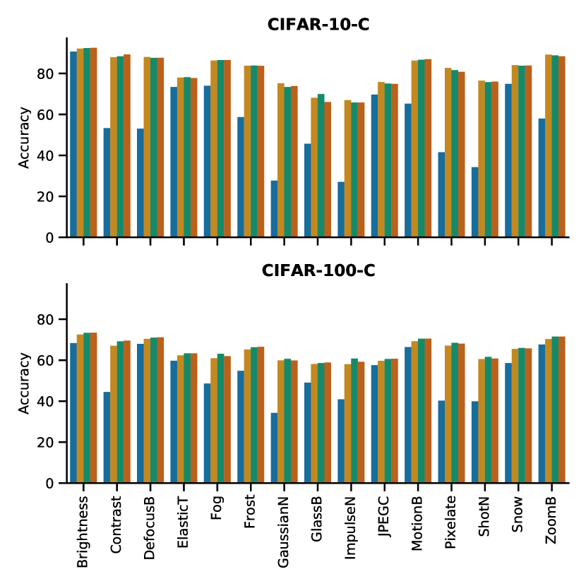
Figure 1: Performance comparisons for CIFAR-10-C and CIFAR-100-C datasets for unadapted, Tent, Augmix, Randaugment variants of our method. Our proposed method, independent of the augmentation strategy used, gives a considerable improvement over the baseline. It is also on par or slightly better than Tent for all corruption categories.

Appendix D Ablations

In this section, we provide ablations of three of the important hyperparameters of our algorithm, number of SGD steps, learning rate, and testing batch size, here. We use the VisDA-C experimental setup and show our results for RandAugment setup with default hyperparameters. The other hyperparameters remain the defaults set in the main paper, unless they are being ablated on. The three ablations refer to Figure 2. For all the ablations in this section, we show performance as $\%$ accuarcy on the test set.

D.1 Number of SGD update steps

The loss function in Equation 4 is minimized over several SGD steps, and we plot the evolution of performance with number of steps. We see an asymptotic rise in the performance with number of steps, and we use $5$ steps for all other steps. However this increases the run-time of our algorithm at test time, and thus we recommend a number dependent on the running time requirements.

D.2 Learning rate

We change our learning rate on a logarithmic scale from $10^{-6}$ to $10^{-1}$, and we see that our method is reasonably robust to the choice, with the best learning rate is around $10^{-4}$.

D.3 Batch size

We find that our method is stable for range of batch sizes, but does have a lower threshold around $16$. We hypothesize this is due to training the normalization layers in the networks used. We were limited by the hardware available to run larger batch sizes.

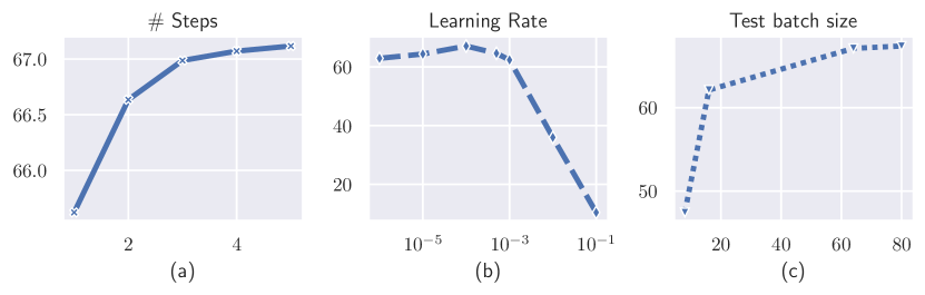
Figure 2: Ablation experiments. With an unadapted performance of $44.1\%$, we show the importance of the factors. We see an asymptotically improving performance with the number of SGD steps used. In (b), we see that our method is relatively stable over a wide range of learning rates. Our method is dependent on batch size as in (c). The necessity of larger batch size can pose constraints on the direct applicability of our method. This method

D.4 Ablation of terms in Equation 4

Our loss function in Equation 4 is a summation of two terms. Here we present the results obtained by considering each of them terms. We see that in Table 5, the usage of Equation 1 leads to a performance higher than that of Tent, and the combination of Equations 1 and 3 leads to better results, albeit at a higher run-time requirement.

Table 5: Ablations of the loss terms in Equation 4.

Unadapted	$\mathcal{L}_{cons}$	$\mathcal{L}$
44.08	63.41	67.1

D.5 Augmentation parameters

We vary the augmentation hyperparameters for both RandAugment, and AugMix in Figures 3 and 4. For this, we show results on CIFAR-10-C for each of the corruptions. We show results with only consistency loss (Equation 1), and width and brightness of each circle represents the overall final accuracy. We find that for nearly all the corruptions, lower amount of augmentation results in better performance compared to ones with higher augmentation. We hypothesize this is because lower intensity augmentations result in samples closer to the input sample, and thus results in samples from the image manifold.

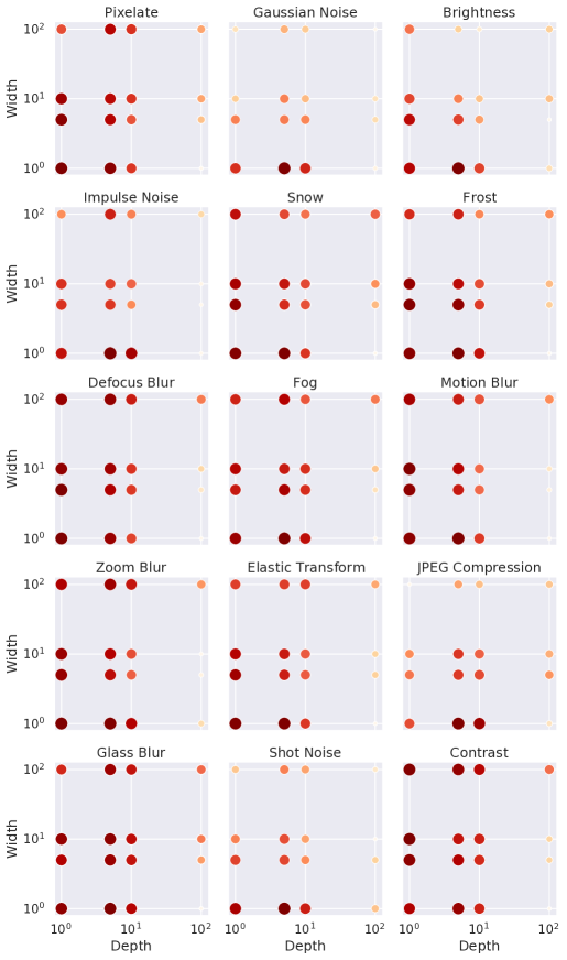
Figure 3: AugMix hyperparameters for CIFAR-10-C. We see that lesser augmentations result in better results.

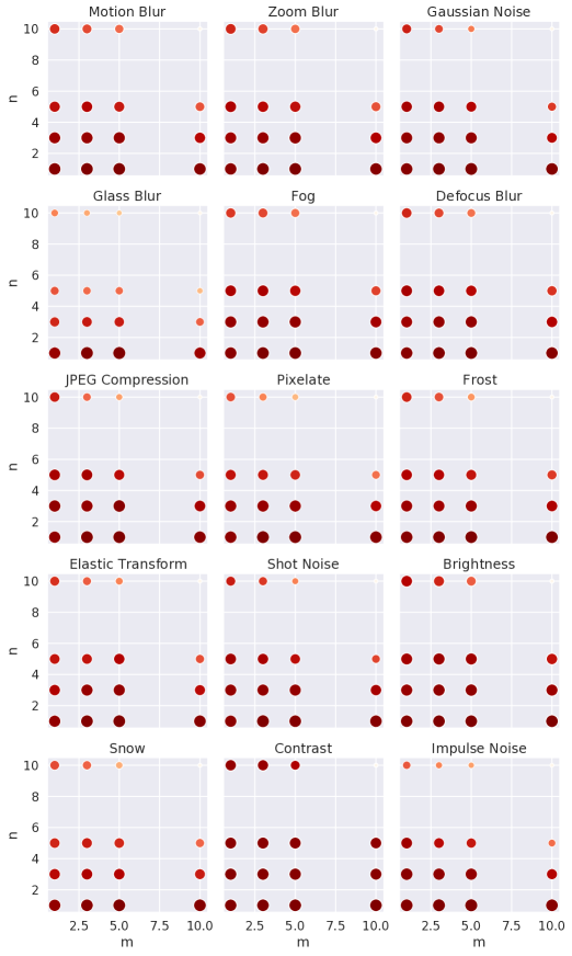
Figure 4: RandAugment hyperparameters for CIFAR-10-C. We see that lesser augmentations result in better results.

References

- Bachman et al. [2014] Philip Bachman, Ouais Alsharif, and Doina Precup. Learning with pseudo-ensembles. In Proceedings of the 27th International Conference on Neural Information Processing Systems - Volume 2, NIPS’14, page 3365–3373, Cambridge, MA, USA, 2014. MIT Press.
- Berthelot et al. [2019] David Berthelot, Nicholas Carlini, Ian Goodfellow, Nicolas Papernot, Avital Oliver, and Colin A Raffel. Mixmatch: A holistic approach to semi-supervised learning. Advances in Neural Information Processing Systems, 32, 2019.
- Bobu et al. [2018] Andreea Bobu, Eric Tzeng, Judy Hoffman, and Trevor Darrell. Adapting to continuously shifting domains, 2018. URL https://openreview.net/forum?id=BJsBjPJvf.
- Bousquet and Elisseeff [2002] Olivier Bousquet and André Elisseeff. Stability and generalization. The Journal of Machine Learning Research, 2:499–526, 2002.
- Chaudhari et al. [2017] P. Chaudhari, A. Choromańska, Stefano Soatto, Y. LeCun, Carlo Baldassi, C. Borgs, J. Chayes, Levent Sagun, and R. Zecchina. Entropy-sgd: Biasing gradient descent into wide valleys. ArXiv, abs/1611.01838, 2017.
- Chen et al. [2020] Ting Chen, Simon Kornblith, Mohammad Norouzi, and Geoffrey Hinton. A simple framework for contrastive learning of visual representations. arXiv preprint arXiv:2002.05709, 2020.
- Chidlovskii et al. [2016] Boris Chidlovskii, Stephane Clinchant, and Gabriela Csurka. Domain adaptation in the absence of source domain data. In Proceedings of the 22nd ACM SIGKDD International Conference on Knowledge Discovery and Data Mining, pages 451–460, 2016.
- Croce et al. [2020] Francesco Croce, Maksym Andriushchenko, Vikash Sehwag, Edoardo Debenedetti, Nicolas Flammarion, Mung Chiang, Prateek Mittal, and Matthias Hein. Robustbench: a standardized adversarial robustness benchmark. arXiv preprint arXiv:2010.09670, 2020.
- Cubuk et al. [2019a] E. D. Cubuk, B. Zoph, D. Mane, V. Vasudevan, and Q. V. Le. Autoaugment: Learning augmentation strategies from data. In 2019 IEEE/CVF Conference on Computer Vision and Pattern Recognition (CVPR), pages 113–123, Los Alamitos, CA, USA, jun 2019a. IEEE Computer Society. doi: 10.1109/CVPR.2019.00020. URL https://doi.ieeecomputersociety.org/10.1109/CVPR.2019.00020.
- Cubuk et al. [2019b] Ekin D. Cubuk, Barret Zoph, Jonathon Shlens, and Quoc V. Le. Randaugment: Practical data augmentation with no separate search. CoRR, abs/1909.13719, 2019b. URL http://arxiv.org/abs/1909.13719.
- Elsayed et al. [2018] Gamaleldin F. Elsayed, Dilip Krishnan, Hossein Mobahi, Kevin Regan, and Samy Bengio. Large margin deep networks for classification. In Proceedings of the 32nd International Conference on Neural Information Processing Systems, NIPS’18, page 850–860, Red Hook, NY, USA, 2018. Curran Associates Inc.
- Ganin et al. [2016] Yaroslav Ganin, Evgeniya Ustinova, Hana Ajakan, Pascal Germain, Hugo Larochelle, François Laviolette, Mario March, and Victor Lempitsky. Domain-adversarial training of neural networks. Journal of Machine Learning Research, 17(59):1–35, 2016. URL http://jmlr.org/papers/v17/15-239.html.
- Grandvalet and Bengio [2005] Yves Grandvalet and Yoshua Bengio. Semi-supervised learning by entropy minimization. Advances in Neural Information Processing Systems, 17:529–536, 2005.
- He et al. [2016] Kaiming He, Xiangyu Zhang, Shaoqing Ren, and Jian Sun. Deep residual learning for image recognition. In 2016 IEEE Conference on Computer Vision and Pattern Recognition (CVPR), pages 770–778, 2016. doi: 10.1109/CVPR.2016.90.
- Hendrycks and Dietterich [2019] Dan Hendrycks and Thomas Dietterich. Benchmarking neural network robustness to common corruptions and perturbations. Proceedings of the International Conference on Learning Representations, 2019.
- Hendrycks et al. [2020] Dan Hendrycks, Norman Mu, Ekin D. Cubuk, Barret Zoph, Justin Gilmer, and Balaji Lakshminarayanan. AugMix: A simple data processing method to improve robustness and uncertainty. Proceedings of the International Conference on Learning Representations (ICLR), 2020.
- Huang et al. [2018] Sheng-Wei Huang, Che-Tsung Lin, Shu-Ping Chen, Yen-Yi Wu, Po-Hao Hsu, and Shang-Hong Lai. Auggan: Cross domain adaptation with gan-based data augmentation. In Proceedings of the European Conference on Computer Vision (ECCV), September 2018.
- Huang et al. [2020] W. Ronny Huang, Zeyad Emam, Micah Goldblum, Liam Fowl, Justin K. Terry, Furong Huang, and Tom Goldstein. Understanding generalization through visualizations. In Jessica Zosa Forde, Francisco Ruiz, Melanie F. Pradier, and Aaron Schein, editors, Proceedings on ”I Can’t Believe It’s Not Better!” at NeurIPS Workshops, volume 137 of Proceedings of Machine Learning Research, pages 87–97. PMLR, 12 Dec 2020. URL https://proceedings.mlr.press/v137/huang20a.html.
- Jo and Bengio [2017] Jason Jo and Yoshua Bengio. Measuring the tendency of cnns to learn surface statistical regularities. arXiv preprint arXiv:1711.11561, 2017.
- Keskar et al. [2016] Nitish Shirish Keskar, Dheevatsa Mudigere, Jorge Nocedal, Mikhail Smelyanskiy, and Ping Tak Peter Tang. On large-batch training for deep learning: Generalization gap and sharp minima. arXiv preprint arXiv:1609.04836, 2016.
- Krizhevsky et al. [2012] Alex Krizhevsky, Ilya Sutskever, and Geoffrey E Hinton. Imagenet classification with deep convolutional neural networks. Advances in neural information processing systems, 25:1097–1105, 2012.
- Laine and Aila [2017] Samuli Laine and Timo Aila. Temporal ensembling for semi-supervised learning. In 5th International Conference on Learning Representations, ICLR 2017, Toulon, France, April 24-26, 2017, Conference Track Proceedings. OpenReview.net, 2017. URL https://openreview.net/forum?id=BJ6oOfqge.
- Leen [1994] Todd K. Leen. From data distributions to regularization in invariant learning. In NIPS, pages 223–230, 1994. URL http://papers.nips.cc/paper/925-from-data-distributions-to-regularization-in-invariant-learning.
- Li et al. [2020] Rui Li, Qianfen Jiao, Wenming Cao, Hau-San Wong, and Si Wu. Model adaptation: Unsupervised domain adaptation without source data. In 2020 IEEE/CVF Conference on Computer Vision and Pattern Recognition (CVPR), pages 9638–9647, 2020. doi: 10.1109/CVPR42600.2020.00966.
- Liang et al. [2020] Jian Liang, Dapeng Hu, and Jiashi Feng. Do we really need to access the source data? source hypothesis transfer for unsupervised domain adaptation. In International Conference on Machine Learning (ICML), pages 6028–6039, July 13–18 2020.
- Mishra et al. [2021] Samarth Mishra, Kate Saenko, and Venkatesh Saligrama. Surprisingly simple semi-supervised domain adaptation with pretraining and consistency. CoRR, abs/2101.12727, 2021. URL https://arxiv.org/abs/2101.12727.
- Miyato et al. [2018] Takeru Miyato, Shin-ichi Maeda, Masanori Koyama, and Shin Ishii. Virtual adversarial training: a regularization method for supervised and semi-supervised learning. IEEE transactions on pattern analysis and machine intelligence, 41(8):1979–1993, 2018.
- Nado et al. [2021] Zachary Nado, Shreyas Padhy, D. Sculley, Alexander D’Amour, Balaji Lakshminarayanan, and Jasper Snoek. Evaluating prediction-time batch normalization for robustness under covariate shift, 2021.
- Novak et al. [2018] Roman Novak, Yasaman Bahri, Daniel A. Abolafia, Jeffrey Pennington, and Jascha Sohl-Dickstein. Sensitivity and generalization in neural networks: an empirical study. In International Conference on Learning Representations, 2018. URL https://openreview.net/forum?id=HJC2SzZCW.
- Peng et al. [2018] Xingchao Peng, Ben Usman, Neela Kaushik, Dequan Wang, Judy Hoffman, and Kate Saenko. Visda: A synthetic-to-real benchmark for visual domain adaptation. In Proceedings of the IEEE Conference on Computer Vision and Pattern Recognition Workshops, pages 2021–2026, 2018.
- Rasmus et al. [2015] Antti Rasmus, Harri Valpola, Mikko Honkala, Mathias Berglund, and Tapani Raiko. Semi-supervised learning with ladder networks. In Proceedings of the 28th International Conference on Neural Information Processing Systems - Volume 2, NIPS’15, page 3546–3554, Cambridge, MA, USA, 2015. MIT Press.
- Ratner et al. [2017] Alexander J. Ratner, Henry R. Ehrenberg, Zeshan Hussain, Jared Dunnmon, and Christopher Ré. Learning to compose domain-specific transformations for data augmentation. In Proceedings of the 31st International Conference on Neural Information Processing Systems, NIPS’17, page 3239–3249, Red Hook, NY, USA, 2017. Curran Associates Inc. ISBN 9781510860964.
- Recht et al. [2019] Benjamin Recht, Rebecca Roelofs, Ludwig Schmidt, and Vaishaal Shankar. Do ImageNet classifiers generalize to ImageNet? In Kamalika Chaudhuri and Ruslan Salakhutdinov, editors, Proceedings of the 36th International Conference on Machine Learning, volume 97 of Proceedings of Machine Learning Research, pages 5389–5400. PMLR, 09–15 Jun 2019. URL http://proceedings.mlr.press/v97/recht19a.html.
- Sajjadi et al. [2016] Mehdi Sajjadi, Mehran Javanmardi, and Tolga Tasdizen. Regularization with stochastic transformations and perturbations for deep semi-supervised learning. In Proceedings of the 30th International Conference on Neural Information Processing Systems, NIPS’16, page 1171–1179, Red Hook, NY, USA, 2016. Curran Associates Inc. ISBN 9781510838819.
- Schneider et al. [2020] Steffen Schneider, Evgenia Rusak, Luisa Eck, Oliver Bringmann, Wieland Brendel, and Matthias Bethge. Removing covariate shift improves robustness against common corruptions. CoRR, abs/2006.16971, 2020.
- Shorten and Khoshgoftaar [2019] Connor Shorten and T. Khoshgoftaar. A survey on image data augmentation for deep learning. Journal of Big Data, 6:1–48, 2019.
- Sun et al. [2020] Yu Sun, Xiaolong Wang, Zhuang Liu, John Miller, Alexei Efros, and Moritz Hardt. Test-time training with self-supervision for generalization under distribution shifts. In Hal Daumé III and Aarti Singh, editors, Proceedings of the 37th International Conference on Machine Learning, volume 119 of Proceedings of Machine Learning Research, pages 9229–9248. PMLR, 13–18 Jul 2020. URL http://proceedings.mlr.press/v119/sun20b.html.
- Tarvainen and Valpola [2017] Antti Tarvainen and Harri Valpola. Mean teachers are better role models: Weight-averaged consistency targets improve semi-supervised deep learning results. In Proceedings of the 31st International Conference on Neural Information Processing Systems, NIPS’17, page 1195–1204, Red Hook, NY, USA, 2017. Curran Associates Inc. ISBN 9781510860964.
- Teja and Fleuret [2021] Prabhu Teja and Francois Fleuret. Uncertainty reduction for model adaptation in semantic segmentation. In Proceedings of the IEEE/CVF Conference on Computer Vision and Pattern Recognition (CVPR), pages 9613–9623, June 2021.
- Toldo et al. [2020] Marco Toldo, Andrea Maracani, Umberto Michieli, and Pietro Zanuttigh. Unsupervised domain adaptation in semantic segmentation: a review. Technologies, 8(2):35, 2020.
- Vergara et al. [2012] Alexander Vergara, Shankar Vembu, Tuba Ayhan, Margaret A. Ryan, Margie L. Homer, and Ramón Huerta. Chemical gas sensor drift compensation using classifier ensembles. Sensors and Actuators B: Chemical, 166-167:320–329, 2012. ISSN 0925-4005. doi: https://doi.org/10.1016/j.snb.2012.01.074. URL https://www.sciencedirect.com/science/article/pii/S0925400512002018.
- Volpi et al. [2018] Riccardo Volpi, Pietro Morerio, Silvio Savarese, and Vittorio Murino. Adversarial feature augmentation for unsupervised domain adaptation. In Proceedings of the IEEE Conference on Computer Vision and Pattern Recognition, pages 5495–5504, 2018.
- Vu et al. [2019] Tuan-Hung Vu, Himalaya Jain, Maxime Bucher, Mathieu Cord, and Patrick Pérez. Advent: Adversarial entropy minimization for domain adaptation in semantic segmentation. In CVPR, 2019.
- Wang et al. [2021] Dequan Wang, Evan Shelhamer, Shaoteng Liu, Bruno Olshausen, and Trevor Darrell. Tent: Fully test-time adaptation by entropy minimization. In International Conference on Learning Representations, 2021. URL https://openreview.net/forum?id=uXl3bZLkr3c.
- Weng [2021] Lilian Weng. Contrastive representation learning. lilianweng.github.io/lil-log, 2021. URL https://lilianweng.github.io/lil-log/2021/05/31/contrastive-representation-learning.html.
- Yeo et al. [2021] Teresa Yeo, Oğuzhan Fatih Kar, and Amir Zamir. Robustness via cross-domain ensembles. arXiv, 2021.
- Zagoruyko and Komodakis [2016] Sergey Zagoruyko and Nikos Komodakis. Wide residual networks. In Edwin R. Hancock Richard C. Wilson and William A. P. Smith, editors, Proceedings of the British Machine Vision Conference (BMVC), pages 87.1–87.12. BMVA Press, September 2016. ISBN 1-901725-59-6. doi: 10.5244/C.30.87. URL https://dx.doi.org/10.5244/C.30.87.
- Zbontar et al. [2021] Jure Zbontar, Li Jing, Ishan Misra, Yann LeCun, and Stéphane Deny. Barlow twins: Self-supervised learning via redundancy reduction. arXiv preprint arXiv:2103.03230, 2021.
- Zhuang et al. [2021] Fuzhen Zhuang, Zhiyuan Qi, Keyu Duan, Dongbo Xi, Yongchun Zhu, Hengshu Zhu, Hui Xiong, and Qing He. A comprehensive survey on transfer learning. Proceedings of the IEEE, 109(1):43–76, 2021. doi: 10.1109/JPROC.2020.3004555.