TeSLA: Test-Time Self-Learning With Automatic Adversarial Augmentation

Abstract

Most recent test-time adaptation methods focus on only classification tasks, use specialized network architectures, destroy model calibration or rely on lightweight information from the source domain. To tackle these issues, this paper proposes a novel Test-time Self-Learning method with automatic Adversarial augmentation dubbed TeSLA for adapting a pre-trained source model to the unlabeled streaming test data. In contrast to conventional self-learning methods based on cross-entropy, we introduce a new test-time loss function through an implicitly tight connection with the mutual information and online knowledge distillation. Furthermore, we propose a learnable efficient adversarial augmentation module that further enhances online knowledge distillation by simulating high entropy augmented images. Our method achieves state-of-the-art classification and segmentation results on several benchmarks and types of domain shifts, particularly on challenging measurement shifts of medical images. TeSLA also benefits from several desirable properties compared to competing methods in terms of calibration, uncertainty metrics, insensitivity to model architectures, and source training strategies, all supported by extensive ablations. Our code and models are available on GitHub.

1 Introduction

Deep neural networks (DNNs) perform exceptionally well when the training (source) and test (target) data follow the same distribution. However, distribution shifts are inevitable in real-world settings and propose a major challenge to the performance of deep networks after deployment. Also, access to the labeled training data may be infeasible at test time due to privacy concerns or transmission bandwidth. In such scenarios, source-free domain adaptation (SFDA) [25, 1, 23] and test-time adaptation (TTA) methods [39, 19, 28] aim to adapt the pre-trained source model to the unlabeled distributionally shifted target domain while easing access to source data. While SFDA methods have access to all full target data through multiple training epochs (offline setup), TTA methods usually process test images in an online streaming fashion and represent a more realistic domain adaptation. However, most of these methods are applied: (i) only to classification tasks, (ii) evaluated on the non-real-world domain shifts, e.g., the non-measurement shift; (iii) destroy model calibration—entropy minimizing with overconfident predictions [45] on incorrectly classified samples, and (iv) use specialized network architectures or rely on the source dataset feature statistics [28].

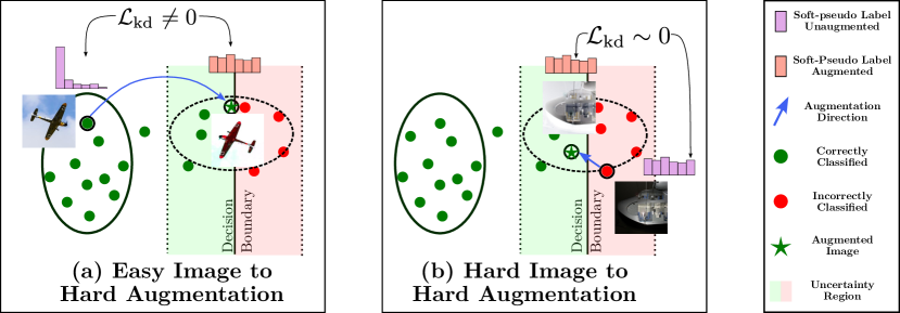
Figure 1: Knowledge distillation with adversarial augmentations. (a) Easy images with confident soft-pseudo labels and (b) Hard images with unconfident soft-pseudo labels are adversarially augmented and pushed to the uncertainty region (high entropy) near the decision boundary. The model is updated for (a) to match its output on the augmented views with non-augmented views of Easy test images using KL-Divergence $\mathcal{L}_{\text{kd}}\neq 0$, while not updated for (b) as $\mathcal{L}_{\text{kd}}\sim 0$ between Hard images and their augmented views.

We address these issues by proposing a new test-time adaptation method with automatic adversarial augmentation called TeSLA, under which we further define realistic TTA protocols. Self-learning methods often supervise the model adaptation on the unlabeled test images using their predicted pseudo-labels. As the model can easily overfit on its own pseudo-labels, a weight-averaged teacher model (slowly updated by the student model) is employed for obtaining the pseudo-labels [41, 47]. The student model is then trained with cross-entropy ($\mathbb{CE}$) loss between the one-hot pseudo-labels and its predictions on the test images. In this paper, we instead propose to minimize flipped cross-entropy between the student model’s predictions and the soft pseudo-labels (notice the reverse order) with the negative entropy of its marginalized predictions over the test images. In Sec. 3, we show that the proposed formulation is an equivalence to mutual information maximization implicitly corrected by the teacher-student knowledge distillation via pseudo-labels, yielding performance improvement on various test-time adaptation protocols and compared to the basic $\mathbb{CE}$ optimization (cf. ablation in Fig. 5-(1)).

Motivated by teacher-student knowledge distillation, another central tenet of our method is to assist the student model during adaptation in improving its performance on the hard-to-classify (high entropy) test images. For this purpose, we propose learning automatic adversarial augmentations (see Fig. 1) as a proxy for simulating images in the uncertainty region of the feature space. The model is then updated to ensure consistency between predictions of high entropy augmented images and soft-pseudo labels from the respective non-augmented versions. Consequently, the model is self-distilled on Easy test images with confident soft-pseudo labels (Fig. 1a). In contrast, the model update on Hard test images is discarded (Fig. 1b), resulting in better class-wise feature separation.

In summary, our contributions are: (i) we propose a novel test-time self-learning method based on flipped cross-entropy (f-$\mathbb{CE}$) through the tight connection with the mutual information between the model’s predictions and the test images; (ii) we propose an efficient plug-in test-time automatic adversarial augmentation module used for online knowledge distillation from the teacher to the student network that consistently improves the performance of test-time adaptation methods, including ours; and (iii) TeSLA achieves new state-of-the-art results on several benchmarks, from common image corruption to realistic measurement shifts for classification and segmentation tasks. Furthermore, TeSLA outperforms existing TTA methods in terms of calibration and uncertainty metrics while making no assumptions about the network architecture and source domain’s information, e.g., feature statistics or training strategy.

2 Related Work

In general, domain adaptation methods aim to distill knowledge from source data that are well-generalizable to target data and relax the assumption of i.i.d. between source and target datasets. To circumvent expensive and cumbersome annotation of new target data, unsupervised domain adaptation (UDA) emerges, and there has been a large corpus of UDAs[32, 51, 17, 13] to match the distribution of domains on both labeled source data and unlabeled target data. Nonetheless, the above-mentioned methods demand source data to achieve the domain adaptation process, which is often impractical in real-world scenarios, e.g., due to privacy restrictions. The above issue motivates research into source-free domain adaptation (SFDA) [26, 25, 1, 23] and test-time training or adaptation (TTA) [39, 19, 28, 45], which are more closely relevant to our problem setup.

SFDA approaches formulate domain adaptation through pseudo labeling [26, 23], target feature clustering [49], synthesizing extra training samples [24], or feature restoration [12]. SHOT [26] proposed feature clustering via information maximization while incorporating pseudo-labeling as additional supervision. BAIT [48] leverages the fixed source classifier as source anchors and uses them to achieve feature alignment between the source and target domain. CPGA [35] proposed the SFDA method based on matching feature prototypes between source and target domains. AaD-SFDA [50] proposed to optimize an objective by encouraging prediction consistency of local neighbors in feature space. Nevertheless, SFDA methods require apriori access to all target data in advance, and the current pseudo-labeling approach, e.g., SHOT [26], used offline pseudo-label refinement on a per-epoch basis. In a more realistic domain adaptation scenario, SFDA will still be incompetent to perform inference and adaptation simultaneously.

TTA methods [45, 4] propose alleviating the domina shift by online (or streaming) adapting a model at test time. Still, we argue that there are ambiguities over the problem setup of TTA in the literature, particularly on whether sequential inference on target test data is feasible upon arrival [19, 45] or whether training objectives must be adapted [28, 40]. TTT [40] proposed fine-tuning the model parameters via rotation classification task as a proxy. On-target adaptation [44] used pseudo-labeling and contrastive learning to initialize the target-domain feature; each performed independently in their method. T3A [19] utilized pseudo-labeling to adjust the classifier prototype. More recently, TTAC [39] leveraged the clustering scheme to match target domain clusters to source domain categories. Nevertheless, existing TTA methods rely on specialized neural network architectures or only update a fraction of model weights yielding limited performance gain on the target data. For instance, TENT [45] proposed updating affine parameters in the batchnorm layers of convolutional neural networks (CNN), while AdaContrast [4] and SHOT [26] used an additional weight normalization classification layer with a projection head. In contrast, we show our methods’ superiority for various neural network architectures, including CNNs and vision transformers (ViTs) [11], without additional architectural requirements and different source model training strategies. Moreover, we update all model parameters, and our method is stable over a wide range of hyper-parameters, e.g., learning rate.

Test time augmentation methods [29, 2] are another popular line of domain adaptation research. GPS [29] learns optimal augmentation sub-policies by combining image transformations of RandAugment [10] that minimize calibrated log-likelihood loss [2] on the validation set. OptTTA [42] optimized the magnitudes of augmentation sub-policies using gradient descent to maximize mutual information and match feature statistics over augmented images. Though effective, these methods [29, 42, 46] are computationally expensive as all augmentation sub-policies need to be evaluated, making their real-time application difficult. Instead, our proposed adversarial augmentation policies can be learned online and are several orders faster than the existing learnable test-time augmentation strategies, e.g., [42].

3 Methodology

Overview. We first introduce our flipped cross-entropy (f-$\mathbb{CE}$) loss through the tight connection with the mutual information between the model’s predictions and the test images. (Sec. 3.1). Using this equivalence, we derive our test-time loss function that implicitly incorporates teacher-student knowledge distillation. In Sec. 3.2, we propose to enhance the test-time teacher-student knowledge distillation by utilizing the consistency of the student model’s predictions on the proposed adversarial augmentations with their corresponding refined soft-pseudo labels from the teacher model. We refine the soft-pseudo labels by averaging the teacher model’s predictions on (1) weakly augmented test images; (2) nearest neighbors in the feature space. Furthermore, we propose an efficient online algorithm for learning adversarial augmentations (Sec. 3.3). Finally, in Sec. 3.4, we summarize our online test-time adaptation method, TeSLA, based on self-learning with the proposed automatic adversarial augmentation. The overall framework is shown in Fig. 2.

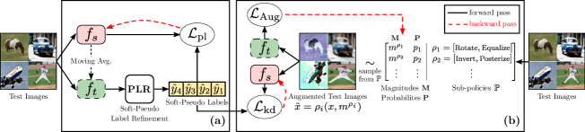
Figure 2: Overview of TeSLA Framework. (a) The student model $f_{s}$ is adapted on the test images by minimizing the proposed test-time objective $\mathcal{L}_{\text{pl}}$. The high-quality soft-pseudo labels required by $\mathcal{L}_{\text{pl}}$ are obtained from the exponentially weighted averaged teacher model $f_{t}$ and refined using the proposed Soft-Pseudo Label Refinement (PLR) on the corresponding test images. The soft-pseudo labels are further utilized for teacher-student knowledge distillation via $\mathcal{L}_{\text{kd}}$ on the adversarially augmented views of the test images. (b) The adversarial augmentations are obtained by applying learned sub-policies sampled i.i.d from $\mathbb{P}$ using the probability distribution $P$ with their corresponding magnitudes selected from $M$. The parameters $M$ and $P$ of the augmentation module are updated by the unbiased gradient estimator (Eq. 13) of the loss $\mathcal{L}_{\text{Aug}}$ computed on the augmented test images.

Problem setup. Given an existing model $f_{\theta_{0}}$, parametrized by $\theta_{0}$ and pre-trained on the inaccessible source data, we aim to improve its performance by updating all its parameters using the unlabeled streaming test data $\mathbf{X}$ during adaptation. Motivated by the concept of mean teacher [41] as the weight-averaged model over training steps that can yield a more accurate model, we build our online knowledge distillation framework upon teacher-student models. We utilize identical network architecture for teacher and student models. Each model $f=h\circ g$ comprises a backbone encoder $g:\mathbf{X}\to\mathbb{R}^{D}$ mapping unlabeled test image $\boldsymbol{x}\in\mathbf{X}$ to the feature representation $\mathbf{z}=g\left(\boldsymbol{x}\right)\in\mathbb{R}^{D}$ and a classifier (hypothesis) head $h:\mathbb{R}^{D}\to\mathbb{R}^{K}$ mapping $\mathbf{z}$ to the class prediction $\boldsymbol{y}\in\mathbb{R}^{K}$, where $D$ and $K$ denote the feature dimension and number of classes. The parameters of teacher $\theta_{t}$ and student $\theta_{s}$ are first initialized from the source model parameters $\theta_{0}$. Then the teacher model’s parameters $\theta_{t}$ are updated from the student model’s parameters $\theta_{s}$ using an exponential moving average (EMA) with momentum coefficient $\alpha$ as: $\theta_{t}\leftarrow\alpha\cdot\theta_{t}+(1-\alpha)\cdot\theta_{s}$. Following [26], we freeze the classifier $h$’s parameters and only update the encoder $g$’s parameters during test-time adaptation.

3.1 Rationale Behind the f-CE Objective

We start by analyzing the rationale behind the proposed f-$\mathbb{CE}$ loss and its benefit for self-learning through the tight connection with the mutual information between the model’s predictions and unlabeled test images. Before that, we first define the notations.

Notations. We define the random variables of unlabeled test images and the predictions from the student model $f_{s}$ as $\mathbf{X}$ and $\mathbf{Y}$ and those of the teacher model $f_{t}$’s soft pseudo-label predictions as $\hat{\mathbf{Y}}$. Furthermore, let $p_{\mathbf{Y}}$ denotes the marginal distribution over $\mathbf{Y}$, $p_{\left(\mathbf{Y},\mathbf{X}\right)}$ be the joint distribution of $\mathbf{Y}$ and $\mathbf{X}$, and $p_{\mathbf{Y}\mid\mathbf{X}}$ be the conditional distribution of $\mathbf{Y}$ given $\mathbf{X}$. Then, the entropy of $\mathbf{Y}$ and the conditional entropy of $\mathbf{Y}$ given $\mathbf{X}$ can be defined as $\mathcal{H}\left(\mathbf{Y}\right):=\mathbb{E}_{p_{\mathbf{Y}}}\left[-\log p_{\mathbf{Y}}\left(\mathbf{Y}\right)\right]$ and $\mathcal{H}\left(\mathbf{Y}\mid\mathbf{X}\right):=\mathbb{E}_{p_{\left(\mathbf{Y},\mathbf{X}\right)}}\left[-\log p_{\mathbf{Y}\mid\mathbf{X}}\left(\mathbf{Y}\mid\mathbf{X}\right)\right]$, respectively. Besides, let the flipped cross-entropy (f-$\mathbb{CE}$) given $\mathbf{X}$ be $\mathcal{H}\left(\mathbf{Y};\hat{\mathbf{Y}}\mid\mathbf{X}\right):=\mathbb{E}_{{p_{\left(\mathbf{Y},\mathbf{X}\right)}}}\left[-\log p_{\hat{\mathbf{Y}}\mid\mathbf{X}}\left(\mathbf{Y}\mid\mathbf{X}\right)\right]$.

Self-learning and mutual information. Based on the above definitions, the f-$\mathbb{CE}$ between $\mathbf{Y}$ and $\hat{\mathbf{Y}}$ conditioned over $\mathbf{X}$ has the tight connection with the mutual information $\mathcal{I}\left(\mathbf{Y};\mathbf{X}\right)$ between unlabeled test images $\mathbf{X}$ and the predictions from the student model $\mathbf{Y}$ as follows:

$$\mathcal{H}\left(\mathbf{Y};\hat{\mathbf{Y}}\mid\mathbf{X}\right)=\mathcal{H}\left(\mathbf{Y}\mid\mathbf{X}\right)+\mathcal{D}_{\text{KL}}\left(\mathbf{Y}\parallel\hat{\mathbf{Y}}\mid\mathbf{X}\right)$$ (1)

$$=-\mathcal{I}\left(\mathbf{Y};\mathbf{X}\right)+\mathcal{H}\left(\mathbf{Y}\right)+\mathcal{D}_{\text{KL}}\left(\mathbf{Y}\parallel\hat{\mathbf{Y}}\mid\mathbf{X}\right)$$

This implies that minimizing the f-$\mathbb{CE}$ ($\mathcal{H}\left(\mathbf{Y};\hat{\mathbf{Y}}\mid\mathbf{X}\right)$ in Eq. 1) and maximizing the entropy of class-marginal prediction $\mathcal{H}\left(\mathbf{Y}\right)$ is equivalent to maximizing the mutual information between the test images and the student model’s predictions $\mathcal{I}\left(\mathbf{Y};\mathbf{X}\right)$ with a correction KL-divergence term $\mathcal{D}_{\text{KL}}\left(\mathbf{Y}\parallel\hat{\mathbf{Y}}\mid\mathbf{X}\right)$ involving soft-pseudo labels as:

$$\underbrace{\mathcal{H}\left(\mathbf{Y};\hat{\mathbf{Y}}\mid\mathbf{X}\right)}_{\text{{f-$\mathbb{CE}$}}}-\mathcal{H}\left(\mathbf{Y}\right)=-\underbrace{\mathcal{I}\left(\mathbf{Y};\mathbf{X}\right)}_{\text{Mutual Info.}}+\mathcal{D}_{\text{KL}}\left(\mathbf{Y}\parallel\hat{\mathbf{Y}}\mid\mathbf{X}\right)$$ (2)

Thus, minimizing the left side of Eq. 2 with respect to the student model’s parameters $\theta_{s}$ allows the student model to cluster test images using mutual information and criterion-corrected knowledge distillation from soft-pseudo labels. Using the above formulation, we define the following test-time objective to train the student model $f_{s}$ on a batch of $B$ test images $X=\{\boldsymbol{x}_{1},\dots,\boldsymbol{x}_{B}\}$ with their corresponding soft-pseudo labels from teacher model $\hat{Y}=\{\hat{\boldsymbol{y}}_{1},\dots,\hat{\boldsymbol{y}}_{B}\}$.

$$\mathcal{L}_{\text{pl}}(X,\hat{Y})=-\frac{1}{B}\sum_{i=1}^{B}\sum_{k=1}^{K}f_{s}(\boldsymbol{x}_{i})_{k}\log((\hat{\boldsymbol{y}}_{i})_{k})\\ +\sum_{k=1}^{K}\hat{f_{s}}(X)_{k}\log(\hat{f_{s}}(X))_{k}$$ (3)

where $\hat{f_{s}}(X)=\frac{1}{B}\sum_{i=1}^{B}f_{s}(\boldsymbol{x}_{i})$ denotes the marginal class distribution over the batch of test images $X$.

3.2 Knowledge Distillation via Augmentation

Self-learning from adversarial augmentations. As illustrated in Fig. 1, adversarial augmentations are learned by pushing their feature representations toward the decision boundary (Expansion phase), followed by updating the student model $f_{s}$ to match its prediction on these augmented images with their corresponding soft-pseudo label (Separation phase), yielding better separation of features into their respective classes. In our method setup, we continually learn automatic augmentations of the test images (Sec. 3.3) that are adversarial to the current teacher model $f_{t}$ and enforce consistency between the student model’s $f_{s}$ predictions on the augmented views and the corresponding soft-pseudo labels. Since we freeze the classifier module, $f_{s}$ and $f_{t}$ share the common decision boundary. Let $\tilde{\boldsymbol{x}}$ denote the learned adversarial augmented view of $\boldsymbol{x}$ and $\hat{\boldsymbol{y}}$ denote the corresponding soft-pseudo label. We minimize the following knowledge distillation loss $\mathcal{L}_{\text{kd}}$ using KL-divergence to distill knowledge from the teacher model to the student model:

$$\mathcal{L}_{\text{kd}}(\tilde{\boldsymbol{x}},\hat{\boldsymbol{y}})=\mathcal{D}_{\text{KL}}(\hat{\boldsymbol{y}}\|f_{s}(\tilde{\boldsymbol{x}}))$$ (4)

Soft pseudo label refinement (PLR). We refine the quality of soft pseudo-labels and the feature representations by averaging the teacher model’s outputs on multiple weakly augmented image views $\rho_{w}(\boldsymbol{x})$ (via flipping, cropping augmentations) of the same test image $\boldsymbol{x}$ as follows:

$$\mathbf{z}_{t},\boldsymbol{y}_{t}\leftarrow\mathbb{E}_{\mathbf{u}\in\rho_{w}(\boldsymbol{x})}[g_{t}(\mathbf{u}),h_{t}(g_{t}(\mathbf{u}))]$$ (5)

The refined feature representations $\mathbf{z}_{t}$ and the softmaxed pseudo labels $\boldsymbol{y}_{t}$ from the encoder $g_{t}$ and the classifier $h_{t}$ are further stored in an online memory queue $\mathbf{Q}$ of fixed size. The final soft pseudo-label is computed by averaging the refined soft pseudo-labels of $n$-nearest neighbors of the current test image in the feature space as follows:

$$\begin{gathered}\mathbf{Q}[\arg\max(\boldsymbol{y}_{t})]\text{.append}(\{\mathbf{z}_{t},\boldsymbol{y}_{t}\})\\ \hat{\boldsymbol{y}}=\frac{1}{n}\sum\mathcal{N}_{\mathbf{Q},n}(\mathbf{z}_{t})\end{gathered}$$ (6)

where $\mathbf{Q}$ denotes an online memory of class-balanced queues (with size $|\mathbf{Q}[\arg\max(\boldsymbol{y}_{t})]|\leq N_{\mathbf{Q}}$) of the refined feature representations and the softmaxed label predictions on the previously seen test images, and $\mathcal{N}_{\mathbf{Q},n}(\mathbf{z}_{t})$ denotes soft labels of $n$-nearest neighbors of $\mathbf{z}_{t}$ from $\mathbf{Q}$.

3.3 Learning Adversarial Data Augmentation

This section presents our efficient online method for learning adversarial data augmentation for the current teacher $f_{t}$. We first introduce our adversarial augmentation search space. Then, we describe our differentiable strategy to optimize and sample adversarial augmentations that push the feature representations of the test images toward the uncertain region in the close vicinity of the decision boundary.

Policy search space. Let $\mathbb{O}$ be a set of all image transformation operations $\mathcal{O}:\mathbb{R}^{H\times W\times 3}\rightarrow\mathbb{R}^{H\times W\times 3}$ defined in our search space. In particular, we use image transformations Auto-Contrast, Equalize, Invert, Solarize, Posterize, Contrast, Brightness, Color, ShearX, ShearY, TranslateX, TranslateY, Rotate, and Sharpness. Each transformation $\mathcal{O}$ is specified with its magnitude parameter $m\in[0,1]$. Since the output of some image operations may not be conditional on its magnitude (e.g., Equalize) or may not be differentiable (e.g., Posterize), for such image operations, we use the straight-through gradient estimate w.r.t. each pixel as: $\partial\mathcal{O}\left(\boldsymbol{x}_{ij}\right)/\partial m=\mathbf{1}$ for magnitude optimization.

We define a sub-policy $\rho$ as a combination of $N$ image operations (sub-policy dimension) from $\mathbb{O}$ that is applied sequentially to a given image $\boldsymbol{x}$ as:

$$\rho\left(\boldsymbol{x},m^{\rho}\right)=\mathcal{O}_{1}^{\rho}\cdots\mathcal{O}_{N}^{\rho}\left(\boldsymbol{x},m_{N}^{\rho}\right)$$ (7)

where $m^{\rho}=[m_{1}^{\rho},\dots,m_{N}^{\rho}]$ denotes the magnitude set of the sub-policy $\rho$. We also define $\mathbb{P}=\{\rho_{1},\rho_{2},\dots\}$ as the set of all possible sub-policies.

Policy evaluation. We propose learnable adversarial augmentation, aiming to optimize and sample data augmentations as a proxy for simulating data in the uncertain region of the feature space. Given the teacher model $f_{t}$, a sub-policy $\rho$ with magnitude $m$ is evaluated for a test image $\boldsymbol{x}$ using the following adversarial objective:

$$\mathcal{L}_{\text{aug}}(\boldsymbol{x},\rho)=\sum_{k=1}^{K}f_{t}\left(\tilde{\boldsymbol{x}}\right)\log\left(f_{t}\left(\tilde{\boldsymbol{x}}\right)\right)+\lambda_{1}r(\tilde{\boldsymbol{x}},\boldsymbol{x})$$ (8)

where $\tilde{\boldsymbol{x}}=\rho\left(\boldsymbol{x},m\right)$ denotes the adversarial augmented image and $r\left(\cdot,\cdot\right)$ regularizes augmentation severity. The hyperparameter $\lambda_{1}$ controls the augmentation severity. We optimize the adversarial augmentation loss $\mathcal{L}_{\text{aug}}$ with respect to the sub-policy $\rho$’s parameters. Minimizing $\mathcal{L}_{\text{aug}}$ is equivalent to maximizing the entropy of the teacher model’s prediction on the augmented image $\tilde{\boldsymbol{x}}$, thus pushing its feature representation towards the decision boundary (first term). For the augmentation regularization (second term), we use the mean squared distance function between the teacher encoder’s $L$ internal layers’ activations of the adversarial augmentation and non-augmented versions of image $\boldsymbol{x}$ defined as:

$$r(\tilde{\boldsymbol{x}},\boldsymbol{x})=\frac{1}{L}\sum_{l=1}^{L}\|\mu_{l}(\tilde{\boldsymbol{x}})-\mu_{l}(\boldsymbol{x})\|^{2}$$ (9)

where $\mu_{l}\left(\cdot\right)$ denotes the mean activation of the $l^{th}$ layer of the teacher encoder $g_{t}$.

Policy optimization. Let $M=[m^{\rho_{1}},\dots,m^{\rho_{\|\mathbb{P}\|}}]$ denote the set of magnitudes $m^{\rho}$ of all sub-policies $\rho\in\mathbb{P}$ and $P=[p_{1},\dots,p_{\|\mathbb{P}\|}]$ denote the probability of selecting a sub-policy from $\mathbb{P}$. The expected policy evaluation loss (Eq. 8) for an image $\boldsymbol{x}$ over the policy search space is given by:

$$\mathbb{E}[\mathcal{L}_{\text{aug}}(\boldsymbol{x})]=\sum_{i=1}^{\|\mathbb{P}\|}p_{i}\cdot\mathcal{L}_{\text{aug}}(\boldsymbol{x},\rho_{i})$$ (10)

Evaluating the gradient of $\mathbb{E}[\mathcal{L}_{\text{aug}}(\boldsymbol{x})]$ w.r.t. $M$ and $P$ can become computationally expensive as $\|\mathbb{P}\|\sim\binom{\|\mathbb{O}\|}{N}$. Thus, we use the following re-parameterization trick to estimate its unbiased gradient:

$$\nabla\mathbb{E}[\mathcal{L}_{\text{aug}}(x)]=\delta(\boldsymbol{x},\mathbb{P})=\sum_{i=1}^{\|\mathbb{P}\|}\nabla(p_{i}\cdot\mathcal{L}_{\text{aug}}(\boldsymbol{x},\rho_{i}))$$ (11)

$$=\sum_{i=1}^{\|\mathbb{P}\|}p_{i}(\nabla\mathcal{L}_{\text{aug}}(\boldsymbol{x},\rho_{i})+\mathcal{L}_{\text{aug}}(\boldsymbol{x},\rho_{i})\cdot\nabla\log p_{i})$$

Thus, an unbiased estimator of $\delta(\boldsymbol{x},\mathbb{P})$ can be written as:

$$\hat{\delta}(\boldsymbol{x},\rho_{i})=\nabla\mathcal{L}_{\text{aug}}(\boldsymbol{x},\rho_{i})+\mathcal{L}_{\text{aug}}(\boldsymbol{x},\rho_{i})\cdot\nabla\log p_{i}$$ (12)

where index $i$ is sampled from the probability distribution $P$. For an online batch of $B$ test images $\{\boldsymbol{x}_{1},\boldsymbol{x}_{2},\dots,\boldsymbol{x}_{B}\}$, we apply augmentation sub-policies $\{\rho_{i_{1}},\rho_{i_{2}}\dots,\rho_{i_{B}}\}$ from $\mathbb{P}$ where $\{i_{1},i_{2},\dots,i_{B}\}$ are sampled i.i.d from distribution $P$, and update the parameters $P$ and $M$ with the following stochastic gradient update rule:

$$[P,M]\leftarrow[P,M]-\frac{\gamma}{B}\sum_{j=1}^{B}\hat{\delta}(\boldsymbol{x}_{j},\rho_{i_{j}})$$ (13)

where $\gamma$ is the learning rate. We set $\gamma=0.1$ for all experiments without the need for hyperparameter tuning.

3.4 Self-Learning With Adversarial Augmentation

We minimize the following overall objective $\mathcal{L}_{\text{TeSLA}}$ for training the student model $f_{s}$ on a batch of $B$ test images $X=\{\boldsymbol{x}_{1},\dots,\boldsymbol{x}_{B}\}$ and their adversarial augmented views $\tilde{X}=\{\tilde{\boldsymbol{x}}_{1},\dots,\tilde{\boldsymbol{x}}_{B}\}$ with the corresponding refined soft-pseudo labels from the teacher model $\hat{Y}=\{\hat{\boldsymbol{y}}_{1},\dots,\hat{\boldsymbol{y}}_{B}\}$:

$$\mathcal{L}_{\text{TeSLA}}(X,\tilde{X},\hat{Y})=\mathcal{L}_{\text{pl}}(X,\hat{Y})+\frac{\lambda_{2}}{B}\sum_{i=1}^{B}\mathcal{L}_{\text{kd}}(\tilde{\boldsymbol{x}}_{i},\hat{\boldsymbol{y}}_{i})$$ (14)

where $\lambda_{2}$ is a hyper-parameter for the knowledge distillation. The adversarial augmented views $\tilde{X}$ are obtained by sampling i.i.d. augmentation sub-policies from $\mathbb{P}$ for every test image in $X$ with probability $P$ and applying the corresponding magnitude from $M$. Concurrently, we also optimize $M$ and $P$ using the policy optimization mentioned in Sec. 3.3.

4 Experiments

4.1 Datasets and Experimental Settings

We evaluate and compare TeSLA against state-of-the-art (SOTA) test-time adaptation algorithms for both classification and segmentation tasks under three types of test-time distribution shifts resulting from (1) common image corruption, (2) synthetic to real data transfer, and (3) measurement shifts on medical images. The latter is characterized by a change in medical imaging systems, e.g., different scanners across hospitals or various staining techniques.

TTA protocols. We adopt the TTA protocols in [39] and categorize competing methods based on two factors: (i) source training objective and (ii) sequential or non-sequential inference. First, unlike [39], we use Y to indicate if access to the source domain’s information, e.g., feature statistics is possible or if the source training objective is allowed to be modified; otherwise, we use N. Next, we use O to indicate a one-pass adaptation and evaluation protocol (one epoch) for sequential test data and M to show a multi-pass adaptation on all test data and inference after several epochs. Thus, we end up with four possible TTA protocols, namely N-M, Y-M, N-O, and Y-O. Unlike previous works [28, 39], TeSLA does not rely on any source domain feature distribution, yielding two realistic TTA protocols: N-M and N-O.

Hyperparameters for all experiments. We set $\lambda_{1}=\lambda_{2}=1.0$ for all experiments (cf. ablation in Appendix E). For the adversarial augmentation module, we use sub-policy dimension $N=2$ (except for VisDA-C [33], $N=4/3$ for N-O/N-M protocols) (cf. Appendix E) and Adam optimizer [22]. For pseudo-label refinement (PLR), we use five weak augmentations composed of random flips and resize crop. More details of hyperparameters used for each experiment can be found in Appendix A.

Common image corruptions. To evaluate TeSLA’s efficacy for the classification task, we use CIFAR10-C/CIFAR100-C [16] and large-scale ImageNet-C [16] datasets each containing 19 types of corruptions applied to the clean test set with five levels of severity. We perform validation on 4 out of 19 types of corruption (Spatter, Gaussian Blur, Speckle Noise, Saturate) to select hyperparameters and test on the remaining 15 corruptions at the maximum severity level of 5. Following [28], we train the ResNet50 [15] on the clean CIFAR10/CIFAR100/ImageNet training set and adapt it to classify the unlabeled corrupted test set.

Synthetic to real data adaption. We use challenging and large-scale VisDA-C, and VisDA-S [33] datasets for evaluating synthetic-to-real data adaptation at test-time for classification and segmentation tasks, respectively. Following [4, 26], we adapt the ResNet101 network pre-trained on synthetic images to classify 12 vehicle classes on the photo-realistic images of VisDA-C. While for VisDA-S, we adapt the DeepLab-v3 [5] backbone pre-trained on synthetic GTA5 [36] to the Cityscapes [7] to segment 19 classes.

Measurement shifts on medical images. We access TeSLA on staining variations for the tissue type classification of hematoxylin & eosin (H&E) stained patches from colorectal cancer tissue slides. We use MobileNetV2 [38] trained on the source Kather-19 dataset [20] and adapt it to the target Kather-16 dataset [21] on four tissue categories: tumor, stroma, lymphocyte, and mucosa. We also evaluate TeSLA for variations in scanners and imaging protocols in multi-site medical images on two magnetic resonance imaging (MRI) datasets for the segmentation task, namely the multi-site prostate MRI [27] and spinal cord grey matter segmentation (SCGM) [34]. Following [42], we adapt the U-Net [37] from site 1 to sites {2,3,4} of the spinal cord dataset, and from sites {A,B} to sites {D,E,F} of the prostate dataset.

Competing baselines. We compare TeSLA with the following SFDA and TTA baselines, including direct inference of the trained source model on the target test data without adaptation (Source). We also implement the SFDA-based pseudo-labeling baselines from a basic pseudo-labeling approach (PL) to the SHOT approach [26] based on training the feature extraction module by adopting the information maximization loss to make globally diverse but individually certain predictions on the target domain. For recent TTA methods, we compare our method against TTT++ [28], AdaContrast [4], CoTTA [47], basic TENT [45] and BN [18] as representative methods based on feature distribution alignment via stored statistics, contrastive learning, augmentation-averaged predictions, entropy minimization, and batch normalization statistic. Furthermore, we compare TeSLA to more recent methods based on test-time augmentation policy learning, OptTTA [42], and anchor clustering TTAC [39]. By default,  [26, 18, 4] follow the N-M protocol, and we adapt them to the N-O protocol, while  [45, 42, 47], by default, follow the N-O protocol and adapt them to the N-M protocol setting. Using source features distribution, TTAC and TTT++ follow Y-O and Y-M. We report error rates on classification tasks and Mean Intersection over Union (mIoU)/ Dice scores on segmentation tasks. For consistency across baselines and TTA protocols, we do not use any specialized model architectures (e.g., projection head, weight-normalized classifier layer) for SHOT [26] and AdaContrast [4].

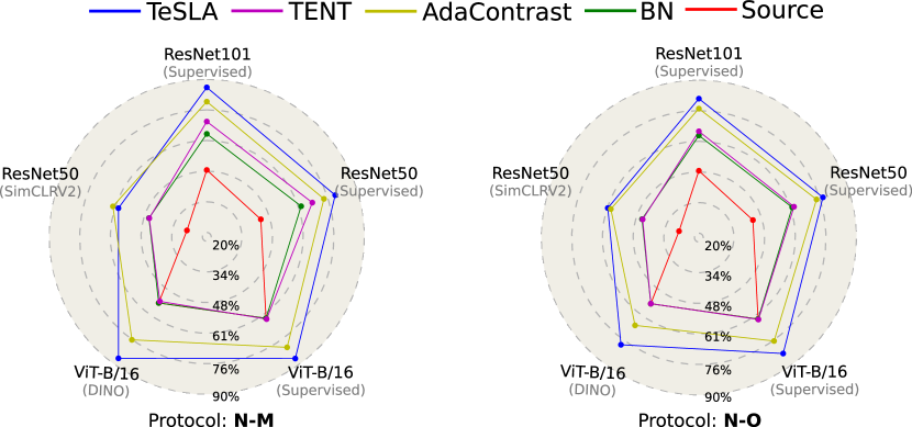
(a)

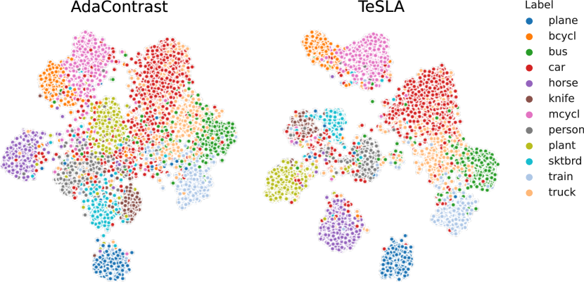
(b)

Figure 3: Ablation experiments on the VisDA-C. (a) Source training strategy and model architecture. TeSLA outperforms the competing TTA methods across varied source training strategies (Supervised, SimCLRV2[6], and DINO[3]) and model architectures (ResNet50, ResNet101 [15], and ViT-B/16[11]) using the same set of hyperparameters for both protocols (N-O/N-M). Each vertex represents the mean class avg accuracy over 3 seeds. (b) t-SNE visualization [43] comparison of feature embeddings for AdaContrast [4] and TeSLA.

Table 1: Comparison of SOTA TTA methods under different protocols evaluated on CIFAR-10/100-C, ImageNet-C, VisDA-C and Kather-16 datasets. We report the average error computed over 15 test corruptions for the common image corruption shifts. We also report Class Avg. in % error rates for synthetic-to-real and measurement shifts over 3 and 10 seeds, respectively.

Method	Protocol	Common Image Corruptions						Syn-to-Real		Measurement Shift
		CIFAR10-C		CIFAR100-C		ImageNet-C		VisDA-C		Kather-16
		O	M	O	M	O	M	O	M	O	M
Source	N	29.1		60.4		81.8		51.5		32.0
BN [30, 18]	N	15.6	15.4	43.7	43.3	67.7	67.6	35.4	35.0	18.3	18.2
TENT [45]	N	14.1	12.9	39.0	36.5	57.4	54.2	33.5	29.3	16.2	12.0
SHOT [26]	N	13.9	14.2	39.2	38.7	68.7	68.2	29.4	24.5	14.7	12.0
AdaContrast [4]	N	-						23.1	20.2	-
TTT++ [28]	Y	15.8	9.8	44.4	34.1	59.3	-	35.2	34.1	16.7	7.9
TTAC [39]	Y	13.4	9.4	41.7	33.6	58.7	-	32.2	31.1	9.6	5.5
TeSLA	N	12.5	9.7	38.2	32.9	55.0	51.5	17.8	13.5	9.2	3.3
TeSLA-s	Y	12.1	9.7	37.3	32.6	53.1	-	24.0	17.9	9.9	3.1

4.2 Results

Classification task. In Table 1, we summarize the average (Avg) classification error rates (%) of TeSLA against several SOTA SFDA and TTA baselines on the common image corruptions of CIFAR10-C, CIFAR100-C, ImageNet-C; synthetic to real data domain shifts of VisDA-C; and measurement shifts on the Kather-16 dataset. We also report per-class top-1 accuracies for VisDA-C and Kather-16 datasets and corruption-wise error rates on CIFAR-10-C/CIFAR-100-C and ImageNet-C datasets in Appendix B. TeSLA easily surpasses all competing methods under the protocols N-O and N-M on all the datasets. In particular, TeSLA outperforms the second-best baseline under N-O/N-M protocol by a (%) margin 1.4/3.2 on CIFAR10-C, 0.8/3.6 on CIFAR100-C, 2.4/2.7 on ImageNet-C, 5.3/6.7 on VisDA-C, and 5.5/8.7 on the Kather-16 datasets. Despite not utilizing any source feature statistic, TeSLA (N-O/N-M) is either competitive or surpasses TTAC[39] and TTT++[28] (Y-O/Y-M) that benefit from the source dataset feature statistics during adaptation. Including the global source feature alignment module of TTAC with TeSLA (TeSLA-s) could further improve its performance under (Y-O/Y-M) protocols for slight domain shifts (e.g., common image corruptions). We report the results of AdaContrast for VisDA-C only as the implementation for other datasets are not provided. We do not report TeSLA-s results on ImageNet-C under the Y-M protocol, as previous baselines were evaluated only Y-O protocol.

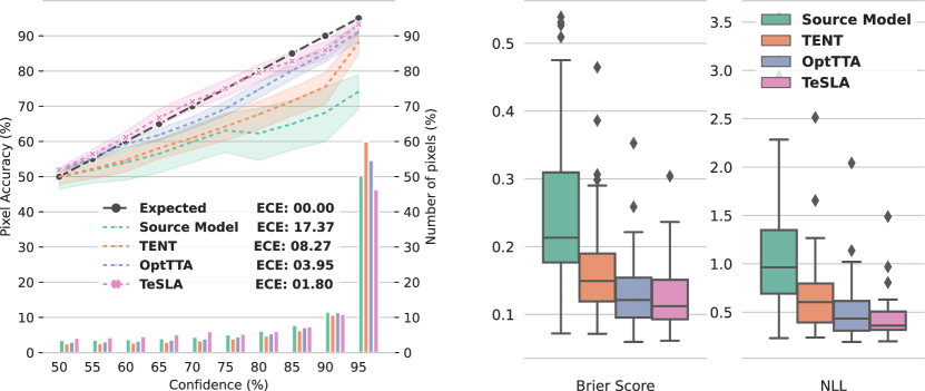
Figure 4: Model calibration and uncertainty estimation. Model calibration using reliability diagrams [31] and model uncertainty estimation using Brier Score and Negative Log Likelihood (NLL) of the Source Model, TENT[45], OptTTA[42] and, TeSLA on the prostate dataset for test-time adaptation.

Table 2: Semantic segmentation results (Class Avg. mIoU in %) on the VisDA-S (GTA5 $\rightarrow$ Cityscapes) test-time adaptation task.

Protocol		Source	BN[30]	TENT[45]	PL	CoTTA[47]	TeSLA
N	O	35.3	36.7	38.3	38.8	37.0	44.5
N	M		38.4	39.2	38.6	39.9	46.0

Table 3: Semantic segmentation results (Class Avg. volume-wise mean Dice in %) on the cross-site spinal cord and prostate MRI test-time adaptation tasks.

Protocol		Source	BN[30]	TENT[45]	PL	OptTTA[42]	TeSLA
Spinal Cord   $\texttt{Site}\left\{\texttt{1}\right\}\rightarrow\texttt{Sites}\left\{\texttt{2,3,4}\right\}$
N	O	76.0$\pm$11.8	81.6$\pm$8.3	81.1$\pm$9.1	81.7$\pm$8.6	84.1$\pm$4.8	85.3$\pm$5.8
N	M		84.3$\pm$4.8	84.4$\pm$4.7	84.3$\pm$4.7	84.3$\pm$4.4	85.4$\pm$4.4
Prostate   $\texttt{Sites}\left\{\texttt{A,B}\right\}\rightarrow\texttt{Sites}\left\{\texttt{D,E,F}\right\}$
N	O	60.5$\pm$27.0	72.1$\pm$15.2	74.7$\pm$17.9	72.4$\pm$15.2	83.1$\pm$7.7	83.5$\pm$6.5
N	M		73.1$\pm$18.0	81.2$\pm$9.3	81.1$\pm$9.2	83.4$\pm$7.7	84.3$\pm$5.8

Segmentation task. Unlike TeSLA, several TTA methods e.g., AdaContrast[4], SHOT[26], TTT++[28], TTAC[39], have only been evaluated on the classification task. Therefore, we compare TeSLA against the current SOTA TTA methods applied to the segmentation task on synthetic-to-real data transfer of the VisDA-S dataset in Table 2. TeSLA significantly outperforms the competing methods and achieves the best mIOU scores for both N-O and N-M protocols, beating the second-best baseline by a margin of +5.7% and +6.1%, respectively. In Table 3, we compare TeSLA against the recent SOTA test-time augmentation policy method, OptTTA[42] and other TTA baselines for the inter-site adaptation on two challenging MRI datasets mentioned in Sec. 4.1. TeSLA convincingly outperforms all other methods on severe measurement shifts across sites under N-O and N-M protocols.

Computational cost for adversarial augmentations. As shown in Table 4, TeSLA learns the adversarial augmentation in an online manner, and thus its runtime is several orders faster than learnable test-time augmentation OptTTA [42], while comparable to that of static augmentation policies with an additional overhead of only 0.10 GPU hours/epoch on the VisDA-C dataset.

Test-time feature visualization. Fig. 3(b) compares t-SNE projection [43] of the encoder’s features of AdaContrast[4] with TeSLA on the VisDA-C. TeSLA shows better inter-class separation for features than AdaContrast, as supported by an improved silhouette score from $0.149$ to $0.271$.

Model calibration and uncertainty estimation. Entropy minimization-based TTA methods [45, 26] explicitly make the model confident in their predictions, resulting in poor model calibration. For trusting the adapted model, it should output reliable confidence estimates matching its true underlying performance on the test images. Such a well-behaved model is characterized by expected calibration error (ECE) through reliability diagram [31], and uncertainty metrics of brier score and negative log-likelihood (NLL) [14]. In Fig. 4, we plot the reliability diagram (dividing the probability range $\left[0,0.5\right]$ into 10 bins), and uncertainty metrics of the Source model, TENT[45] and OptTTA[42] against TeSLA for the inter-site model adaptation on the prostate dataset [27]. We observe that TeSLA achieves the best model calibration (lowest ECE of 1.80%) and lowest Brier and NLL scores of 0.12 and 0.24 ($p$ $<$ 0.006 against TENT).

Table 4: Performance comparison of adversarial augmentation learned by TeSLA during adaptation against the prior art augmentation methods on runtime (GPU hours/epoch on NVIDIA GeForce RTX 3090) and Class Avg. accuracy in % on the VisDA-C dataset.

Augmentation Type	OptTTA	TeSLA RA[10]	TeSLA AA[8]	TeSLA $N=2$	TeSLA $N=3$
Runtime	4.50	0.05	0.06	0.16	0.18
Class Avg. Acc. (N-O)	-	80.2	81.2	81.5	82.2
Class Avg. Acc. (N-M)	-	84.7	85.7	86.3	86.5

4.3 Ablation Studies

In this section, we scrutinize the roles played by different components of TeSLA. All ablations are performed on the synthetic-to-real test data adaptation of the VisDA-C dataset.

Loss functions for self-learning. We compare TTA performance of our self-learning objective $\mathcal{L}_{\text{pl}}$ with the proposed flipped cross-entropy loss f-$\mathbb{CE}$ and the basic cross-entropy loss $\mathbb{CE}$ in Fig. 5-(1). We do not use the proposed augmentation module and pseudo-label refinement in this experiment. We observe that f-$\mathbb{CE}$ alone improves the accuracy of the Source model in the N-M protocol by +23.1% compared to +16.6% improvement by $\mathbb{CE}$. Using $\mathcal{L}_{\text{pl}}$ (Eq. 3) further improves the accuracy to a margin of +23.8%.

Contribution of individual components: PLR, $\mathcal{L}_{\text{pl}}$, and $\mathcal{L}_{\text{kd}}$. Our test-time objective $\mathcal{L}_{\text{TeSLA}}$ has three components– (i) self-learning loss $\mathcal{L}_{\text{pl}}$, (ii) pseudo-label refinement (PLR), and (iii) knowledge distillation $\mathcal{L}_{\text{kd}}$ with adversarial augmentation. In Fig. 5-(3), we study the effect of accruing individual components to $\mathcal{L}_{\text{TeSLA}}$ (starting from source trained model) for the test-time adaptation accuracy. We observe that $\mathcal{L}_{\text{pl}}$ alone improves the model’s accuracy from 48.5% to 72.3% while adding PLR and $\mathcal{L}_{\text{kd}}$ further boosts it to 81.6% (+9.3) and 86.3% (+4.7), respectively.

PLR: ensembling on weak augmentations (Ens) and nearest neighbor averaging (NN). We also conduct an ablation on the two pseudo-label refinement approaches – (i) ensembling the teacher model’s output on five weak augmentations. (ii) averaging soft pseudo labels of $n=10$ nearest neighbors in the feature space (cf. sensitivity test in Appendix E). Fig. 5-(2) shows that combining both approaches gives better results than using them individually.

Adversarial augmentation. Table 4 shows the benefit of using our adversarial augmentation ($N=2,3$) with TeSLA against (i) RandAugment (RA) [10], (ii) AutoAugment (AA) [9] (optimized for ImageNet), and (iii) OptTTA [42]. We achieve far better Class Avg. accuracy on the VisDA-C at the cost of slight runtime overhead compared to static augmentation policies for protocols (N-O, N-M). In addition, TeSLA augmentation (TeAA) consistently improves the performance of other TTA methods (Table 5).

Table 5: Class Avg. accuracy (%) of TeSLA augmentation (TeAA) with other TTA objectives under N-O protocol on VisDA-C dataset.

TENT	+TeAA	SHOT	+TeAA	AdaContrast	+TeAA
66.5	72.0	70.6	73.1	76.9	79.1

Source training strategies and model architectures. The ablation results (Fig. 3(a)) on the VisDA-C show that TeSLA surpasses competing TTA baselines for different source training strategies, including Supervised and self-supervised (SimCLRV2 [6], DINO[3]). Moreover, we ablate TeSLA over different architectures, ranging from ResNet-50/101[15] to the recent vision transformer ViT-B [11] using the same set of hyperparameters, showing the merits of no reliance on the network architecture or source training strategy.

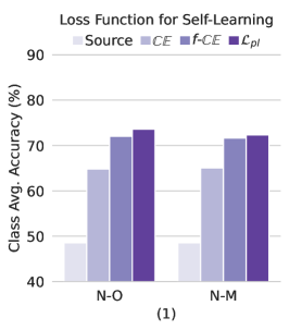
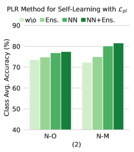
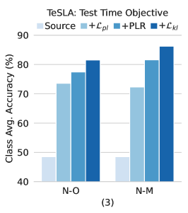
Figure 5: Ablation experiments on the VisDA-C. (left to right) (1) Ablation results for self-learning loss functions, including f-$\mathbb{CE}$, $\mathbb{CE}$, and $\mathcal{L}_{\text{pl}}$; (2) ablation on different PLR methods: ensembling predictions on 5 weak augmentations, averaging predictions of the 10 nearest neighbors in the feature space; (3) ablation on different components of TeSLA’s objective function: $\mathcal{L}_{\text{pl}}$, PLR, and $\mathcal{L}_{\text{kd}}$.

5 Conclusion

We introduced TeSLA, a novel self-learning algorithm for test-time adaptation that utilizes automatic adversarial augmentation. TeSLA is agnostic to the model architecture and source training strategies and gives better model calibration than other TTA methods. Through extensive experiments on various domain shifts (measurement, common corruption, synthetic to real), we show TeSLA’s superiority over previous TTA methods on classification and segmentation tasks. Note that TeSLA assumes class uniformly when implicitly maximizing mutual information and can be improved by incorporating prior, e.g., class label distribution statistics.

Overview. This Appendix provides important additional details about our proposed method TeSLA. In Appendix A, we provide hyperparameters details for each test-time adaptation experiment on the common image corruptions, synthetic-to-real, and medical measurement shift datasets. In Appendix B, we provide additional quantitative results, including class top-1 accuracies for the VisDA-C [33] and Kather-16 [21] datasets and corruption-wise error rates on the CIFAR-10-C/CIFAR-100-C [16], and ImageNet-C [16] datasets. In addition, we also provide segmentation class-wise mean Intersection over Union (mIoU) for the VisDA-S dataset [33] and class average Dice score for different sites of the target test domain on the spinal cord [34] and prostate dataset [27] for the competing test time adaptation methods. All quantitative results are included for both one-pass (O) and multi-pass (M) protocols. Appendix C provides an overall runtime computation cost of TeSLA along with other Test Time adaptation methods on VisDA-C [33] dataset, while Appendix D discusses TeSLA’s equivalence to TENT [45] and [26] without mean teacher and adversarial augmentations. We include additional ablation experiments and hyperparameter sensitivity tests in Appendix E. Finally, we provide other qualitative results, including a sanity check on TeSLA’s adversarial augmentations, uncertainty evaluation, and segmentation visualization in Appendix F.

Appendix A Hyperparameter Settings

Table A.1 and Table A.2 present the hyperparameters’ values of TeSLA used for individual experiments on different classification and segmentation datasets, respectively. These hyperparameters include the batch size $B$, learning rate, optimizer, EMA momentum coefficient $\alpha$, number of epochs for test-time adaptation (M protocol), the number of weak augmentations $|\rho_{w}|$; the number of nearest neighbors $n$; class-wise queue size $N_{Q}$ used by soft pseudo-label refinement (PLR) module, number of image operations for augmentation sub-policy $N$ used by the adversarial augmentation module, the augmentation severity controller coefficient $\lambda_{1}$ and the knowledge distillation coefficient $\lambda_{2}$ for $\mathcal{L}_{\text{kd}}$ loss term.

Table A.1: Hyperparameter setting used for the proposed methods TeSLA/TeSLA-s on different classification datasets.

Hyperparameters	CIFAR10-C		CIFAR100-C		ImageNet-C		VisDA-C		Kather-16
	O	M	O	M	O	M	O	M	O	M
Batch size $B$	128	128	128	128	128	128	128	128	32	32
Learning rate	0.001	0.001	0.001	0.001	0.001	0.001	0.001	0.001	0.005	0.005
Optimizer	Adam	Adam	Adam	Adam	SGD	SGD	SGD	SGD	Adam	Adam
Momentum coefficient $\alpha$	0.99	0.999	0.99	0.999	0.9	0.996	0.9	0.996	0.9	0.96
Number of epochs	1	70	1	70	1	5	1	5	1	70
Number of weak augmented views $|\rho_{w}|$	5	5	5	5	5	5	5	5	5	5
Number of nearest neighbors $n$	1	4	1	1	1	1	10	10	8	8
Class-wise queue size $N_{\mathbf{Q}}$	1	256	1	1	1	1	256	256	32	256
Sub-policy dimension $N$	2	2	2	2	2	2	4	3	2	2
Augmentation severity controller $\lambda_{1}$	1	1	1	1	1	1	1	1	1	1
Knowledge distillation weight $\lambda_{2}$	1	1	1	1	1	1	1	1	1	1

Table A.2: Hyperparameter setting used for the proposed method TeSLA on different segmentation datasets.

Hyperparameters	VisDA-S		Spinal Cord		Prostate
	O	M	O	M	O	M
Batch size $B$	8	8	16	16	16	16
Learning rate	0.001	0.001	0.0002	0.0002	0.0002	0.0002
Optimizer	AdamW	AdamW	AdamW	AdamW	AdamW	AdamW
Momentum coefficient $\alpha$	0.996	0.999	0.996	0.996	0.996	0.996
Number of epochs	1	3	1	5	1	3
Number of weak augmented views $|\rho_{w}|$	3	3	5	5	5	5
Number of nearest neighbors $n$	1	1	1	1	1	1
Class-wise queue size $N_{\mathbf{Q}}$	1	1	1	1	1	1
Sub-policy dimension $N$	3	3	3	3	3	3
Augmentation severity controller $\lambda_{1}$	1	1	1	1	1	1
Knowledge distillation weight $\lambda_{2}$	1	1	1	1	1	1

Appendix B Additional Quantitative Results

In Table B.1, we compare TeSLA against state-of-the-art test-time adaptation methods for the classification task on the Kather-16 dataset. We present the class top-1 accuracies (%) for each of the four tissue categories of tumor, stroma, lymphocyte, and mucosa. In addition, we report the class average accuracy (Avg.).

Furthermore, in Table B.2, we present the corruption-wise average class error rates for different competing test time adaptation baselines, including the proposed TesLA and TeSLA-s on the CIFAR10-C, CIFAR100-C and ImageNet-C. We use the following image corruptions for the evaluation at the maximum severity level of 5: [Gaussian Noise, Shot Noise, Impulse Noise, Defocus Blur, Glass Blur, Motion Blur, Zoom Blur, Snow, Frost, Fog, Brightness, Contrast, Elastic Transformation, Pixelate, JPEG Compression]. We also use the ResNet-50 backbone for all experiments.

In Table B.3, we include the overall and class-wise accuracies for test time adaptation of ResNet-101 trained on synthetic vehicle images (training) and tested on the photo-realistic vehicle images (validation) of the VisDA-C dataset. The photo-realistic images are classified into 12 categories: plane, bicycle, bus, car, horse, knife, motor-cycle, person, plant, skate-board, train, and truck.

In Table B.4, we present segmentation results (class Avg. volume-wise mean %Dice score) for test-time adaptation baselines on two multi-site magnetic resonance imaging (MRI) benchmarks - spinal cord [34] and prostate dataset [27]. For the spinal cord dataset, we report results for test-time adaptation of the U-Net segmentation model trained on site 1 to site 2, site 3, and site 4. Similarly, we report results of the U-Net segmentation model trained on the sites A and B, which are adapted on the sites D, site E, and site F.

Table B.5 presents the results of competing test-time adaptation methods applied to the segmentation adaptation task from the synthetic images of GTA [36] to the photo-realistic images of Cityscapes [7] dataset. We report the class-wise mean Intersection over Union (mIoU) over 19 classes: road, side-walk, building, wall, fence, pole, light, sign, vegetation, terrain, sky, person, rider, car, truck, bus, train, motor-cycle, and bicycle.

Table B.1: Comparison of state-of-the-art TTA methods under different protocols on the Kather-16 dataset. We report the class top-1 accuracies (%) for each of the four classes and the per-class average accuracy (Avg.). Each result is averaged over ten seeds.

Method	Protocol	tumor	stroma	lymphocyte	mucosa	Avg.
Source	N	84.5$\pm$4.0	91.6$\pm$3.0	0.9$\pm$1.2	95.0$\pm$1.3	68.0$\pm$1.3
BN	N-O	89.3$\pm$2.5	85.5$\pm$2.6	61.7$\pm$2.2	90.2$\pm$0.6	81.7$\pm$1.0
Tent	N-O	89.8$\pm$4.0	89.3$\pm$3.4	67.2$\pm$2.2	88.9$\pm$1.0	83.8$\pm$1.8
SHOT	N-O	84.7$\pm$5.7	95.7$\pm$2.0	67.9$\pm$3.9	92.8$\pm$0.8	85.3$\pm$2.5
TTT++	Y-O	82.8$\pm$8.5	85.1$\pm$7.6	73.7$\pm$3.8	91.4$\pm$1.7	83.3$\pm$2.7
TTAC	Y-O	92.6$\pm$2.6	96.6$\pm$1.9	78.3$\pm$4.3	93.9$\pm$1.0	90.4$\pm$1.1
TeSLA	N-O	93.5$\pm$1.8	98.2$\pm$1.2	77.3$\pm$4.1	94.3$\pm$0.7	90.8$\pm$1.1
TeSLA-s	Y-O	90.7$\pm$4.6	98.0$\pm$1.0	77.9$\pm$5.6	94.0$\pm$1.7	90.1$\pm$1.4
BN	N-M	86.3$\pm$3.6	86.1$\pm$1.9	66.9$\pm$1.2	87.7$\pm$0.7	81.8$\pm$1.0
Tent	N-M	96.4$\pm$4.2	99.5$\pm$0.4	62.6$\pm$9.0	93.7$\pm$1.5	88.0$\pm$3.3
SHOT	N-M	84.6$\pm$4.4	98.5$\pm$0.6	77.1$\pm$5.2	91.7$\pm$0.8	88.0$\pm$2.4
TTT++	Y-M	95.6$\pm$1.4	93.9$\pm$2.8	85.2$\pm$5.3	93.6$\pm$1.8	92.1$\pm$2.0
TTAC	Y-M	92.9$\pm$12.6	98.1$\pm$1.1	92.4$\pm$4.7	94.4$\pm$1.8	94.5$\pm$4.7
TeSLA	N-M	97.1$\pm$1.0	99.6$\pm$0.3	94.4$\pm$2.0	95.6$\pm$0.9	96.7$\pm$0.5
TeSLA-s	Y-M	97.4$\pm$0.4	99.5$\pm$0.3	95.1$\pm$2.0	95.7$\pm$1.0	96.9$\pm$0.6

Table B.2: Comparison of state-of-the-art TTA methods under different protocols on common image corruptions datasets, including CIFAR10-C, CIFAR100-C, and ImageNet-C. We report the error rates (%) on 15 test images’ corruptions.

Method	Protocol	Gaus.	Shot	Impu.	Defo.	Glas.	Moti.	Zoom	Snow	Fros.	Fog	Brig.	Cont.	Elas.	Pixe.	Jpeg	Avg.
CIFAR10-C
Source	N	48.7	44.0	57.0	11.8	50.8	23.4	10.8	21.9	28.2	29.4	7.0	13.3	23.4	47.9	19.5	29.1
BN	N-O	18.2	17.2	28.1	9.8	26.6	14.2	8.0	15.5	13.8	20.2	7.9	8.3	19.3	13.3	13.8	15.6
Tent	N-O	16.0	14.8	24.5	9.2	23.8	13.1	7.7	14.9	13.0	16.5	8.2	8.3	17.9	10.9	13.3	14.1
SHOT	N-O	16.5	15.3	23.6	9.0	23.4	12.7	7.5	14.0	12.4	16.1	7.5	8.0	17.4	12.5	13.1	13.9
TTT++	Y-O	18.0	17.1	30.8	10.4	29.9	13.0	9.9	14.8	14.1	15.8	7.0	7.8	19.3	12.7	16.4	15.8
TTAC	Y-O	17.9	15.8	22.5	8.5	23.5	11.2	7.6	11.9	12.9	13.3	6.9	7.6	17.3	12.3	12.6	13.4
TeSLA	N-O	13.3	12.5	20.8	8.8	21.1	11.8	7.3	12.6	11.2	15.6	7.6	7.6	16.2	9.7	11.6	12.5
TeSLA-s	Y-O	13.0	12.2	20.3	8.5	20.8	11.2	7.2	12.0	11.0	15.5	7.3	7.2	15.6	9.1	11.3	12.1
BN	N-M	17.3	16.2	28.0	9.8	26.1	14.0	7.9	16.1	13.7	20.4	8.3	8.3	19.6	11.8	14.0	15.4
Tent	N-M	15.1	13.7	22.2	8.5	22.4	11.8	7.1	12.7	11.9	12.9	7.6	7.6	16.9	9.8	12.6	12.9
SHOT	N-M	15.8	14.8	24.9	9.2	23.6	13.2	7.5	14.5	12.8	17.5	8.1	8.2	18.1	10.8	13.4	14.2
TTT++	Y-M	13.2	11.8	11.1	7.9	16.5	8.9	6.6	9.5	9.7	8.6	5.2	5.6	13.1	8.8	11.1	9.8
TTAC	Y-M	11.6	10.3	15.8	6.8	15.9	7.5	5.8	8.7	9.0	8.5	5.6	5.7	12.7	8.0	9.7	9.4
TeSLA	N-M	10.7	9.8	15.2	7.0	15.8	9.1	6.1	10.0	8.9	10.9	6.0	6.2	13.0	7.9	9.6	9.7
TeSLA-s	Y-M	10.4	9.8	14.9	7.3	16.1	9.0	6.2	9.5	9.1	11.5	5.9	5.8	12.9	7.9	9.5	9.7
CIFAR100-C
Source	N	80.8	77.8	87.8	39.6	82.3	54.2	38.4	54.6	60.2	68.1	28.9	50.9	59.5	72.3	50.0	60.4
BN	N-O	48.2	46.4	61.1	33.8	58.2	41.4	31.9	46.1	42.5	54.7	31.3	33.3	48.4	39.0	39.6	43.7
Tent	N-O	43.3	41.2	52.7	31.2	50.8	36.1	29.3	41.9	38.9	43.6	30.1	31.0	43.5	34.4	36.5	39.0
SHOT	N-O	44.1	41.8	53.3	31.5	50.6	36.0	29.6	40.7	40.1	41.9	29.5	33.6	44.0	34.9	36.6	39.2
TTT++	Y-O	50.2	47.7	66.1	35.8	61.0	38.7	35.0	44.6	43.8	48.6	28.8	30.8	49.9	39.2	45.5	44.4
TTAC	Y-O	47.7	45.7	58.1	32.5	55.3	36.6	31.2	40.3	40.8	44.7	30.0	39.9	47.1	37.8	38.3	41.7
TeSLA	N-O	40.0	38.9	51.5	32.2	49.1	36.9	29.7	40.4	37.4	46.0	29.3	30.7	42.7	32.9	34.6	38.2
TeSLA-s	Y-O	39.1	38.5	50.0	30.6	48.6	35.9	29.1	38.9	36.4	46.2	28.3	29.7	41.9	32.1	33.9	37.3
BN	N-M	47.4	45.5	60.0	33.9	56.9	40.8	31.8	46.4	42.6	54.2	32.3	33.1	48.5	37.2	39.4	43.3
Tent	N-M	41.0	38.4	49.2	30.0	47.4	33.1	28.1	38.1	38.0	37.5	28.3	29.0	41.1	32.8	35.6	36.5
SHOT	N-M	41.6	40.6	51.7	31.4	49.5	36.2	29.3	42.4	38.4	45.4	29.9	31.3	43.1	33.5	36.0	38.7
TTT++	N-M	38.4	37.7	41.3	29.1	44.1	32.9	27.8	34.3	34.4	34.7	25.4	26.6	39.2	32.3	33.6	34.1
TTAC	N-M	37.8	36.8	45.1	28.2	45.3	30.7	26.6	35.3	35.7	36.7	26.8	27.4	39.6	30.6	34.2	33.6
TeSLA	N-M	34.4	33.5	42.2	28.0	41.9	32.1	25.9	35.1	32.6	38.3	25.0	27.4	37.5	28.6	30.6	32.9
TeSLA-s	Y-M	33.9	33.0	42.1	27.5	42.0	31.6	26.1	34.2	32.2	39.4	24.8	26.3	36.8	28.1	30.3	32.6
ImageNet-C
Source	N	97.0	96.3	97.4	82.1	90.3	85.3	77.5	83.4	76.9	76.0	40.9	94.6	83.5	79.1	67.4	81.8
BN	N-O	83.5	82.6	82.9	84.4	84.2	73.1	60.5	65.1	66.3	51.5	34.0	82.6	55.3	50.3	58.7	67.7
Tent	N-O	70.8	68.7	69.1	72.5	73.3	59.3	50.8	53.0	59.1	42.7	32.6	74.5	45.5	41.6	47.8	57.4
SHOT	N-O	77.0	74.6	76.4	81.2	79.3	72.5	61.7	65.7	66.3	55.6	56.0	92.7	57.1	56.3	58.2	68.7
TTAC	Y-O	71.5	67.7	70.3	81.2	77.3	64	54.4	51.1	56.9	45.4	32.6	79.1	46.0	43.7	48.6	59.3
TTT++	Y-O	69.4	66	69.7	84.2	81.7	65.2	53.2	49.3	56.2	44.4	32.8	75.7	43.9	41.6	46.9	58.7
TeSLA	N-O	65.0	62.9	63.5	69.4	69.2	55.4	49.5	49.1	56.6	41.8	33.7	77.9	43.3	40.4	46.6	55.0
TeSLA-s	Y-O	61.4	58.8	60.3	67.3	66.2	54.0	48.2	46.9	53.1	40.9	32.4	81.2	41.1	39.2	44.8	53.1
BN	N-M	83.4	82.6	82.8	84.4	84.2	73.2	60.3	64.9	66.4	51.2	34.0	82.6	54.9	49.9	58.8	67.6
Tent	N-M	66.1	63.7	64.2	68.9	69.6	52.6	47.4	48.4	58.4	39.8	31.6	77.9	41.7	28.7	44.5	54.2
SHOT	N-M	75.8	73.7	73.7	78.3	77.1	71.8	60.9	64.2	66.1	55.4	59.8	95.5	56.1	57.3	58.1	68.2
TeSLA	N-M	62.3	60.9	60.6	64.3	65.7	50.4	46.2	46.1	54.7	39.1	32.2	68.5	40.9	37.5	43.5	51.5

Table B.3: Comparison of state-of-the-art TTA methods under different protocols on the VisDA-C dataset. We report the class top-1 accuracies (%) for each of the 12 classes. We also report the overall accuracy (Acc.) and the per-class average accuracy (Avg.). Each result is averaged over three seeds.

Method

Protocol

plane

bicycle

bus

car

horse

knife

mcycl

person

plant

sktbrd

train

truck

Acc.

Avg.

Source

N

3.8$\pm$4.5

23.3$\pm$0.7

56.0$\pm$3.9

82.5$\pm$0.9

70.8$\pm$3.1

1.6$\pm$0.3

84.4$\pm$1.3

9.1$\pm$2.2

78.0$\pm$5.4

22.1$\pm$3.7

79.3$\pm$2.4

1.6$\pm$0.7

55.6$\pm$0.7

48.5$\pm$1.0

BN

N-O

86.9$\pm$2.2

57.8$\pm$2.3

75.4$\pm$1.2

52.9$\pm$1.3

86.7$\pm$0.6

54.2$\pm$4.0

85.5$\pm$0.9

55.4$\pm$2.0

64.9$\pm$2.7

41.6$\pm$2.3

85.7$\pm$1.2

28.8$\pm$2.5

64.5$\pm$0.3

64.6$\pm$0.5

Tent

N-O

86.9$\pm$2.2

57.7$\pm$3.0

77.4$\pm$1.4

56.8$\pm$1.5

87.3$\pm$0.8

62.4$\pm$3.8

86.6$\pm$0.8

62.9$\pm$2.9

71.2$\pm$1.7

39.9$\pm$2.8

84.8$\pm$1.2

24.7$\pm$3.4

66.3$\pm$0.3

66.5$\pm$0.6

SHOT

N-O

90.5$\pm$1.0

77.0$\pm$0.9

76.2$\pm$0.7

47.5$\pm$0.5

87.9$\pm$0.2

62.1$\pm$4.0

75.9$\pm$0.2

74.4$\pm$1.1

83.3$\pm$0.3

47.0$\pm$6.6

84.2$\pm$0.9

41.6$\pm$0.4

68.6$\pm$0.6

70.6$\pm$1.0

AdaContrast

N-O

95.2$\pm$0.3

78.2$\pm$0.3

81.8$\pm$0.1

67.9$\pm$1.2

94.9$\pm$0.5

87.4$\pm$3.3

87.9$\pm$0.6

82.0$\pm$1.5

90.7$\pm$0.7

36.8$\pm$16.1

88.6$\pm$0.1

31.5$\pm$3.6

76.2$\pm$0.7

76.9$\pm$1.4

TTT++

Y-O

86.4$\pm$1.5

60.5$\pm$2.6

75.7$\pm$2.2

51.7$\pm$3.6

86.5$\pm$0.9

55.3$\pm$2.1

85.2$\pm$2.7

55.8$\pm$1.1

64.5$\pm$2.7

41.3$\pm$2.1

86.4$\pm$1.9

28.4$\pm$2.6

64.4$\pm$0.8

64.8$\pm$0.7

TTAC

Y-O

90.0$\pm$1.2

64.7$\pm$12.5

69.7$\pm$0.9

48.5$\pm$1.7

84.3$\pm$1.8

82.8$\pm$3.6

84.7$\pm$4.1

64.7$\pm$7.2

72.1$\pm$1.3

40.2$\pm$6.3

86.5$\pm$1.2

25.5$\pm$5.6

65.5$\pm$1.6

67.8$\pm$2.1

TeSLA

N-O

95.4$\pm$0.2

87.4$\pm$0.2

83.8$\pm$0.6

70.1$\pm$0.8

95.1$\pm$0.1

90.0$\pm$1.0

84.8$\pm$3.1

83.2$\pm$1.3

93.6$\pm$0.1

67.9$\pm$19.9

85.4$\pm$0.8

49.3$\pm$1.2

80.3$\pm$1.3

82.2$\pm$1.9

TeSLA-s

Y-O

92.0$\pm$0.2

81.2$\pm$2.0

77.1$\pm$1.9

56.5$\pm$0.9

90.2$\pm$0.4

91.0$\pm$0.9

82.9$\pm$1.8

79.8$\pm$0.8

91.3$\pm$0.1

48.9$\pm$3.5

81.2$\pm$1.5

40.1$\pm$2.4

73.5$\pm$0.3

76.0$\pm$0.3

BN

N-M

87.2$\pm$1.4

58.0$\pm$1.1

76.4$\pm$1.4

53.7$\pm$1.9

87.2$\pm$1.3

54.2$\pm$3.6

86.2$\pm$0.3

55.5$\pm$1.6

64.9$\pm$2.3

42.1$\pm$2.7

85.6$\pm$1.3

29.3$\pm$2.2

64.9$\pm$0.1

65.0$\pm$0.4

Tent

N-M

89.1$\pm$2.0

56.4$\pm$5.9

82.4$\pm$1.0

69.2$\pm$0.5

89.3$\pm$1.3

95.2$\pm$0.5

91.4$\pm$0.5

79.5$\pm$1.0

86.1$\pm$0.3

16.3$\pm$1.9

84.7$\pm$0.4

8.4$\pm$3.5

70.9$\pm$0.4

70.7$\pm$0.6

SHOT

N-M

93.9$\pm$0.5

82.6$\pm$0.7

76.6$\pm$0.8

49.7$\pm$1.8

92.0$\pm$0.2

79.0$\pm$21.6

75.3$\pm$2.0

80.9$\pm$2.4

89.5$\pm$0.6

50.5$\pm$19.0

83.8$\pm$0.9

52.2$\pm$1.1

72.7$\pm$1.8

75.5$\pm$3.4

AdaContrast

N-M

95.6$\pm$0.6

82.8$\pm$1.0

76.5$\pm$2.4

72.4$\pm$5.3

96.7$\pm$0.3

91.3$\pm$2.2

88.6$\pm$1.2

85.4$\pm$0.8

95.3$\pm$0.5

30.1$\pm$51.3

93.6$\pm$0.7

48.9$\pm$2.1

79.7$\pm$1.3

79.8$\pm$3.9

TTT++

Y-M

87.2$\pm$2.0

61.8$\pm$2.0

74.7$\pm$1.3

52.7$\pm$3.6

86.1$\pm$1.7

65.0$\pm$7.0

84.9$\pm$2.3

62.1$\pm$6.0

67.2$\pm$1.6

36.6$\pm$1.3

86.2$\pm$0.1

27.1$\pm$3.6

65.3$\pm$0.3

65.9$\pm$1.0

TTAC

Y-M

86.8$\pm$4.2

73.5$\pm$1.3

69.3$\pm$2.1

44.2$\pm$2.5

78.8$\pm$5.1

73.1$\pm$6.7

84.7$\pm$1.6

67.3$\pm$8.6

78.6$\pm$5.6

52.9$\pm$4.1

84.7$\pm$2.6

33.2$\pm$3.9

66.0$\pm$2.0

68.9$\pm$2.4

TeSLA

N-M

96.6$\pm$0.2

91.3$\pm$0.1

85.1$\pm$1.0

69.3$\pm$0.0

96.7$\pm$0.3

97.1$\pm$0.8

88.0$\pm$0.9

85.2$\pm$0.4

96.3$\pm$0.2

87.7$\pm$9.3

87.4$\pm$0.2

57.3$\pm$0.8

83.4$\pm$0.6

86.5$\pm$0.9

TeSLA-s

Y-M

96.1$\pm$0.4

89.4$\pm$0.4

83.0$\pm$0.4

62.4$\pm$0.5

94.4$\pm$0.1

94.5$\pm$1.1

87.3$\pm$0.3

83.3$\pm$0.5

95.5$\pm$0.2

63.9$\pm$14.9

85.7$\pm$0.7

49.4$\pm$3.3

79.3$\pm$1.0

82.1$\pm$1.5

Table B.4: Segmentation results for test-time adaptation methods (class Avg. volume-wise mean Dice score in %) on the spinal cord dataset (site $\left\{\texttt{1}\right\}\rightarrow\texttt{2,3,4}$) and prostate dataset (sites $\left\{\texttt{A,B}\right\}\rightarrow\texttt{D,E,F}$), respectively.

Method	Protocol	Spinal Cord				Prostate
Sites		$\left\{\texttt{1}\right\}\rightarrow\left\{\texttt{2}\right\}$	$\left\{\texttt{1}\right\}\rightarrow\left\{\texttt{3}\right\}$	$\left\{\texttt{1}\right\}\rightarrow\left\{\texttt{4}\right\}$	$\left\{\texttt{1}\right\}\rightarrow\left\{\texttt{2,3,4}\right\}$	$\left\{\texttt{A,B}\right\}\rightarrow\left\{\texttt{D}\right\}$	$\left\{\texttt{A,B}\right\}\rightarrow\left\{\texttt{E}\right\}$	$\left\{\texttt{A,B}\right\}\rightarrow\left\{\texttt{F}\right\}$	$\left\{\texttt{A,B}\right\}\rightarrow\left\{\texttt{D,E,F}\right\}$
		Class Avg.	Class Avg.	Class Avg.	Avg.	Class Avg.	Class Avg.	Class Avg.	Avg.
Source	N	77.4$\pm$6.6	64.8$\pm$11.7	85.9$\pm$3.8	76.0 $\pm$11.8	75.8$\pm$8.9	65.9$\pm$18.5	38.4$\pm$32.3	60.5$\pm$27.0
BN	N-O	85.2$\pm$2.1	70.6$\pm$3.6	88.9$\pm$1.7	81.6$\pm$8.3	75.9$\pm$9.4	74.4$\pm$7.4	65.7$\pm$22.4	72.1$\pm$15.2
TENT	N-O	85.7$\pm$1.8	68.7$\pm$2.8	88.9$\pm$1.7	81.1$\pm$9.1	78.8$\pm$6.2	77.9$\pm$6.9	67.0$\pm$28.4	74.7$\pm$17.9
PL	N-O	85.3$\pm$2.1	71.0$\pm$3.6	88.9$\pm$1.7	81.7$\pm$8.6	76.1$\pm$9.4	74.8$\pm$7.5	66.2$\pm$22.4	72.4$\pm$15.2
OptTTA	N-O	84.4$\pm$2.3	80.2$\pm$5.1	87.5$\pm$2.0	84.1$\pm$4.8	84.9$\pm$6.9	80.3$\pm$8.4	84.0$\pm$6.6	83.1$\pm$7.7
TeSLA	N-O	86.3$\pm$1.5	80.3$\pm$7.3	89.3$\pm$1.4	85.3$\pm$5.8	86.1$\pm$3.3	79.8$\pm$7.5	84.3$\pm$6.3	83.5$\pm$6.5
BN	N-M	85.5$\pm$1.6	78.5$\pm$3.2	88.8$\pm$1.5	84.3$\pm$4.8	77.8$\pm$9.6	77.3$\pm$7.2	63.8$\pm$26.7	73.1$\pm$18.0
TENT	N-M	85.5$\pm$1.6	79.0$\pm$3.3	88.8$\pm$1.5	84.4$\pm$4.7	81.6$\pm$7.7	79.0$\pm$10.4	82.8$\pm$9.2	81.2$\pm$9.3
PL	N-M	85.5$\pm$1.7	78.8$\pm$3.3	88.8$\pm$1.5	84.3$\pm$4.7	81.2$\pm$7.9	79.1$\pm$10.1	82.8$\pm$9.1	81.1$\pm$9.2
OptTTA	N-M	84.3$\pm$2.5	80.7$\pm$4.9	87.7$\pm$2.0	84.3$\pm$4.4	86.2$\pm$5.2	78.6$\pm$8.6	85.0$\pm$6.7	83.4$\pm$7.7
TeSLA	N-M	86.4$\pm$1.7	80.4$\pm$3.2	89.3$\pm$1.7	85.4$\pm$4.4	85.9$\pm$4.0	81.2$\pm$6.7	85.6$\pm$5.4	84.3$\pm$5.8

Table B.5: Segmentation results for test-time adaptation methods (mIoU%) for adaptation from synthetic GTA5 dataset to Cityscapes dataset (O and M protocols).

Method	Protocol	road	sidewalk	building	wall	fence	pole	light	sign	vegetation	terrain	sky	person	rider	car	truck	bus	train	motocycle	bicycle	mIoU
Source	N	72.9	20.0	81.4	21.7	22.9	19.2	25.3	10.6	78.9	26.4	85.9	54.9	20.7	53.0	30.6	16.2	1.9	20.0	7.5	35.3
BN	N-O	84.3	31.8	79.2	24.1	20.5	21.5	23.5	10.5	74.6	32.0	75.3	52.1	14.4	77.6	28.1	20.6	6.0	14.9	6.2	36.7
PL	N-O	84.0	31.1	80.6	25.5	20.7	21.5	24.7	11.4	77.3	34.0	79.4	54.2	17.1	78.3	30.1	21.7	9.7	18.5	8.1	38.3
Tent	N-O	88.0	34.3	80.7	27.7	17.8	19.3	22.1	10.0	80.1	40.5	77.6	51.8	15.7	81.8	32.6	24.0	8.9	18.8	5.8	38.8
CoTTA	N-O	85.8	35.3	79.1	26.5	20.3	19.8	21.7	9.9	76.7	36.2	74.6	53.2	14.4	77.8	29.0	19.3	3.6	13.2	5.8	37.0
TeSLA	N-O	90.4	52.2	82.5	29.6	25.5	28.1	32.5	29.7	79.7	39.0	75.2	59.0	21.3	84.0	29.3	24.6	14.5	23.0	26.1	44.5
BN	N-M	84.3	31.1	80.7	25.4	21.0	22.6	25.6	11.8	76.7	32.7	77.6	54.8	17.2	79.7	29.7	21.7	9.3	18.7	8.5	38.4
PL	N-M	85.1	30.6	80.9	25.7	20.6	21.5	24.7	11.3	77.9	33.9	80.2	54.4	17.4	80.0	30.0	21.9	9.2	19.0	8.3	38.6
Tent	N-M	89.0	35.1	81.0	28.4	17.0	19.5	22.9	9.8	80.8	41.8	76.7	52.4	16.3	83.6	33.0	24.8	7.1	20.6	5.7	39.2
CoTTA	N-M	88.6	40.2	80.6	30.0	20.4	19.2	25.9	16.0	77.1	32.7	75.3	55.7	23.1	82.8	30.1	19.4	9.8	19.9	11.3	39.9
TeSLA	N-M	90.1	51.4	83.1	29.0	27.7	28.7	34.8	34.0	78.7	35.7	73.0	62.0	26.5	83.9	28.5	25.0	25.7	27.3	29.4	46.0

Appendix C Runtime Analysis

We compare the computational runtime cost of several test-time adaptation methods, including BN [18, 30], TTAC [39], SHOT-IM [26], TENT [45], AdaContrast [4] and our proposed method TeSLA in Table C.1. We also include overall TesLA runtimes using static, pre-optimized RandAugment (RA) / AutoAugment (AA) augmentation policies instead of the proposed Adversarial Augmentations.

Table C.1: Runtime (GPU hours) per epoch on GeForce RTX-3090 for ResNet-101 with batch size of 128 on the VisDA-C. RA implies RandAugment [10], AA implies AutoAugment [9].

BN	TTAC	SHOT-IM	TENT	AdaContrast	TeSLA	TeSLA (RA)	TeSLA (AA)
0.04	0.14	0.16	0.05	0.22	0.38	0.27	0.28

Appendix D Equivalence to other Test-Time Objectives

Our proposed flipped cross-entropy loss f-$\mathbb{CE}$ of Eq. 1 without soft-pseudo labels from the teacher is equivalent to entropy minimization of TENT [45], while our final objective $\mathcal{L}_{\text{TeSLA}}$ of Eq. 14 without the knowledge distillation from adversarial augmentation is equivalent to SHOT-IM [26] as $\mathcal{D}_{\text{KL}}\left(\mathbf{Y}\parallel\hat{\mathbf{Y}}\mid\mathbf{X}\right)=0$ when the teacher network is an instant update of the student (momentum $\alpha$ is 0). Thus, without the mean-teacher and adversarial augmentation, our method would have similar shortcomings as that of TENT and SHOT. Incorporating the soft-pseudo labels from the mean teacher alone improves TeSLA’s accuracy on VisDA-C from 82.0% to 86.5%.

Appendix E Sensitivity Tests and Aditional Ablations

E.1 Sensitivity Tests

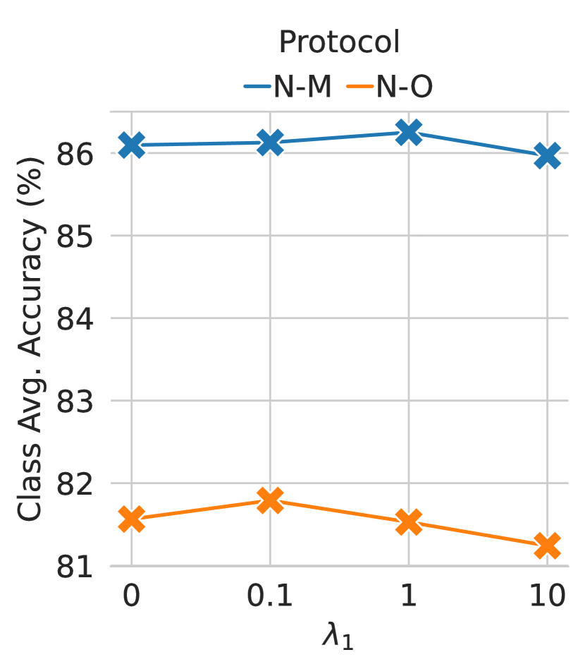
(a)

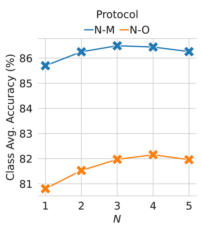
(b)

Figure E.1: Sensitivity test for adversarial augmentation hyperparameters of TeSLA on the VisDA-C dataset for classification task on various TTA protocols. We plot the class Avg. accuracy (%) on the VisDA-C dataset for (a) augmentation severity controller $\lambda_{1}\in\{0,0.1,1,10\}$ and (b) sub-policy dimension $N\in[1,5]$.

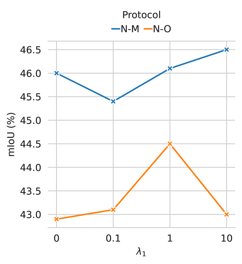
(a)

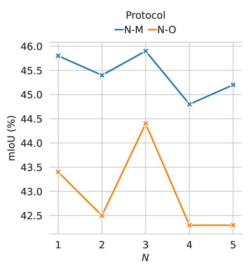
(b)

Figure E.2: Sensitivity test for adversarial augmentation hyperparameters of TeSLA on the VisDA-S dataset for segmentation task on various TTA protocols. We plot the mIoU (%) on the VisDA-S dataset for (a) augmentation severity controller $\lambda_{1}\in\{0,0.1,1,10\}$ and (b) sub-policy dimension $N\in[1,5]$, respectively.

Automatic Adversarial Augmentation.

We additionally provide the sensitivity test results for the hyperparameters of the automatic adversarial augmentation module ($\lambda_{1}$ and sub-policy dimension $N$) on the VisDA-C and VisDA-S datasets. In Fig. E.1, we show how the class average (Avg.) accuracy (%) varies with the hyperparameter $\lambda_{1}$ controlling the severity of augmentations and the sub-policy dimension $N$ on the VisDA-C dataset. Similarly, Fig. E.2 shows the effect of changing $\lambda_{1}$ and $N$ on the segmentation scores measured by mIoU (%) on the VisDA-S dataset. We observe that the performance of our method TeSLA is stable over a wide range of $\lambda_{1}$ and $N$ for both classification and segmentation tasks.

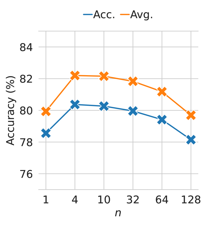
(a)

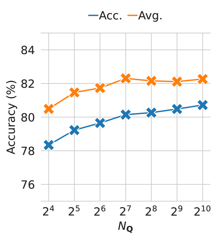
(b)

Figure E.3: Sensitivity test for PLR hyperparameters: (a) the number of nearest neighbors $n$ and (b) the class memory queue size $N_{\mathbf{Q}}$ on the VisDA-C dataset. We report the overall accuracy (Acc.) and the class average accuracy (Avg.) in % on the ViSDA-C under the N-O protocol.

PLR hyperparameters.

We present sensitivity tests for the hyperparameters of the soft pseudo-label refinement (PLR) module. In Fig. E.3, we show the test-time adaptation classification performance of TeSLA on the VisDA-C (N-O) for varying numbers of nearest neighbors $n\in\{1,4,10,32,64,128\}$, and class memory queue size $N_{\mathbf{Q}}\in\{16,32,64,128,256,512,1024\}$. TeSLA outperforms competing baselines under a wide range of choices. Moreover, the number of examples in the queue can be as small as less than 0.5% of the dataset size and still maintains on-par performance.

Fig. E.4 shows the classification performance of TeSLA on the CIFAR10-C and CIFAR100-C and various corruptions [Gaussian Blur, Spatter, Speckle Noise, Saturate] under multiple protocols and the number of weak augmentation for ensembling $|\rho_{w}|\in\{2,3,5,9\}$. These plots show that increasing the number of views decreases the average error rate in both protocols. While we report the results with $|\rho_{w}|=5$ in the main, we observe we could further decrease the error rate with $|\rho_{w}|=9$. However, this choice would multiply the computational cost by two as the number of forward passes is linearly proportional to this hyperparameter. For this reason, we opt $|\rho_{w}|=5$, which gathers the benefit of ensembling and reasonable computational cost.

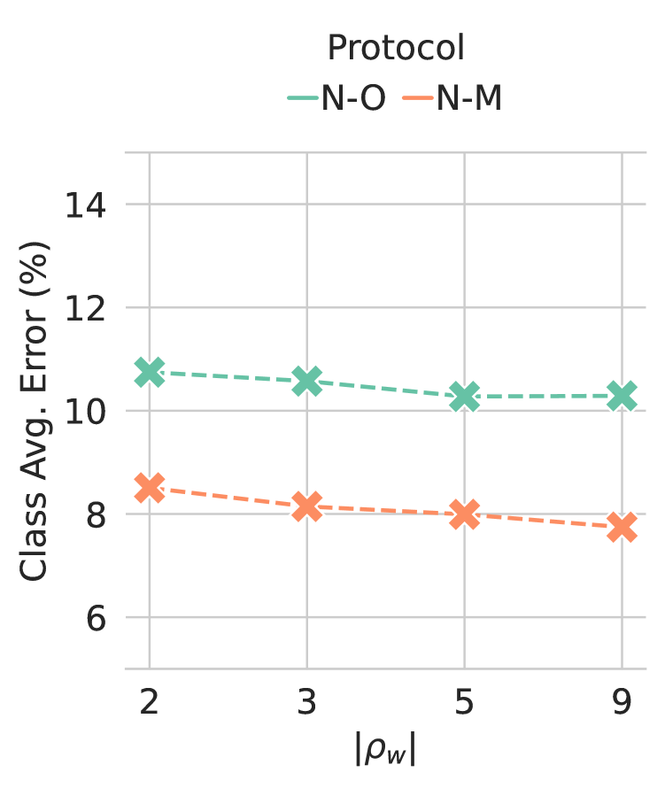
(a) CIFAR10-C

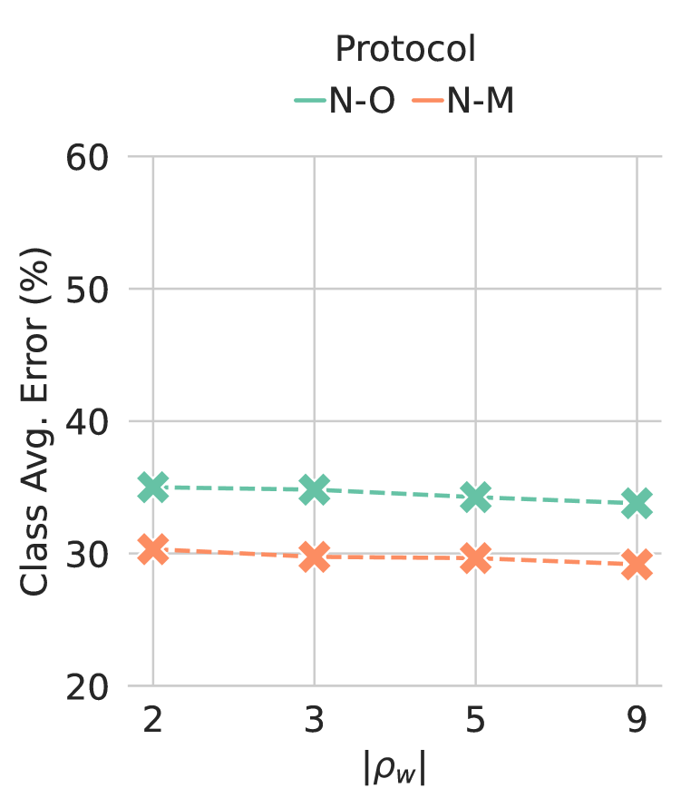
(b) CIFAR100-C

Figure E.4: Sensitivity test on the number of weak augmentation ($|\rho_{w}|$) for ensembling soft-pseudo labels for Soft-Pseudo Label Refinement (PLR) on (a) CIFAR10-C and (b) CIFAR100-C datasets. We report, for each case, the average error rate over 4 validation corruptions.

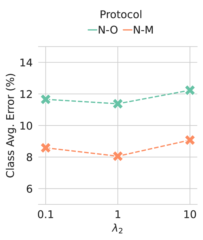
(a) CIFAR10-C

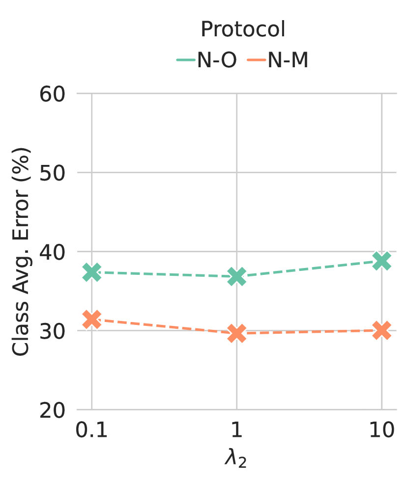
(b) CIFAR100-C

Figure E.5: Sensitivity test on the scalar coefficient $\lambda_{2}$ of $\mathcal{L}_{\text{kd}}$ term of the test time loss $\mathcal{L}_{\text{TeSLA}}$. We report, for each case, the average error rate over the 4 validation corruptions.

Knowledge distillation coefficient.

Finally, we report the sensitivity test results for the knowledge distillation weight $\lambda_{2}$. In Fig. E.5, we show the classification adaptation performance of TeSLA on the CIFAR10-C and CIFAR100-C datasets is not very sensitive to the selection of $\lambda_{2}\in\{0.1,1,10\}$.

E.2 Ablations

EMA coefficient of teacher model.

In Fig. E.6, we show the effect of changing the EMA coefficient $\alpha$ used for updating the teacher model from the student model for the one-pass (O protocol) and multi-pass (M protocol) on the CIFAR10-C and CIFAR100-C datasets. We observe that for the multi-pass protocol (M), decreasing $\alpha$ leads to better performance, while for the one-pass protocol (O), optimal $\alpha$ depends on the number of test images observed in one epoch. If $\alpha$ is large (close to 1.0), the teacher is updated very slowly and thus requires more updates to reach better performance. Therefore, for a one-pass online evaluation, the accuracy decreases. On the other hand, if we set $\alpha$ to a minimal value, it results in unstable convergence.

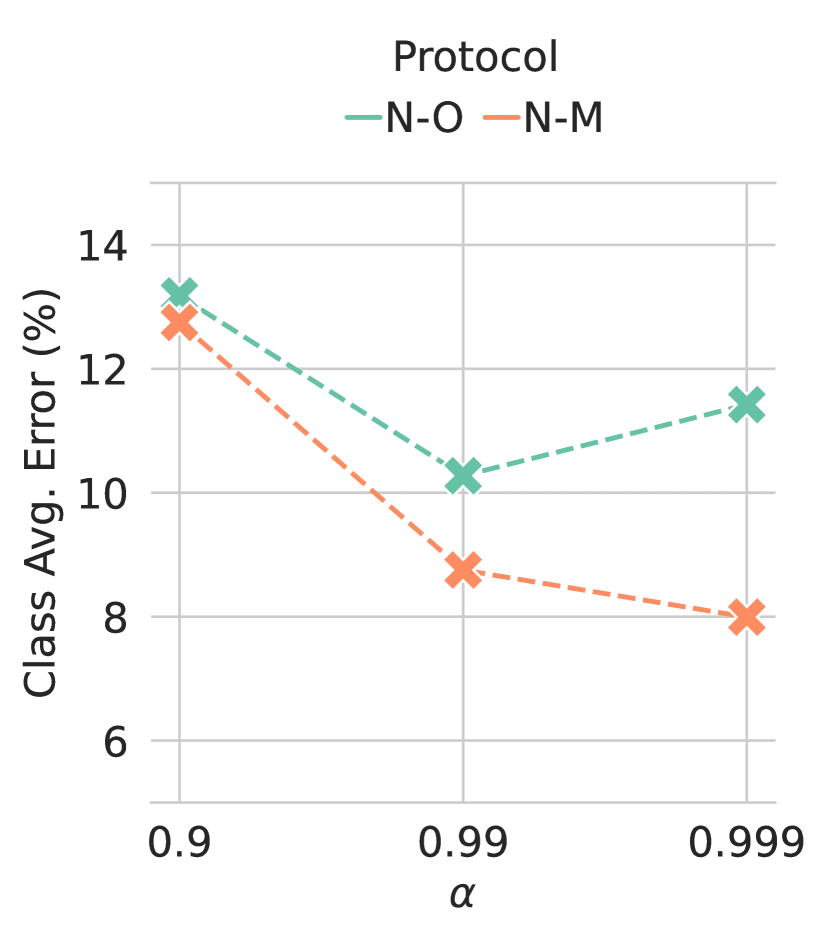
(a) CIFAR10-C

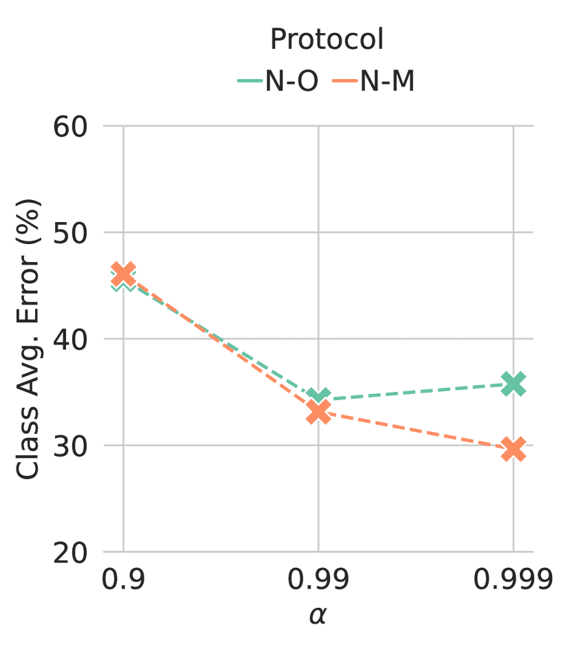
(b) CIFAR100-C

Figure E.6: Sensitivity test on the EMA coefficient of the teacher model $\alpha$ on the (a) CIFAR10-C and (b) CIFAR100-C datasets. We report the average error rate over four corruptions for each dataset.

Batch size and learning rate.

In Fig. E.7, we show the effect of batch size and learning rate on the proposed method TeSLA along with TENT[45], SHOT[26], and TTAC[39] on CIFAR10-C for N-O protocol. We observe that increasing batch size helps reduce test time error rates, and the model performs best with the same batch size used during source model training. Similarly, increasing the learning rate reduces the error rate until it becomes too large for unstable gradient model updates.

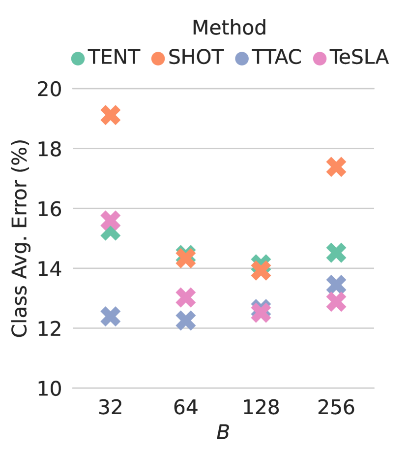
(a)

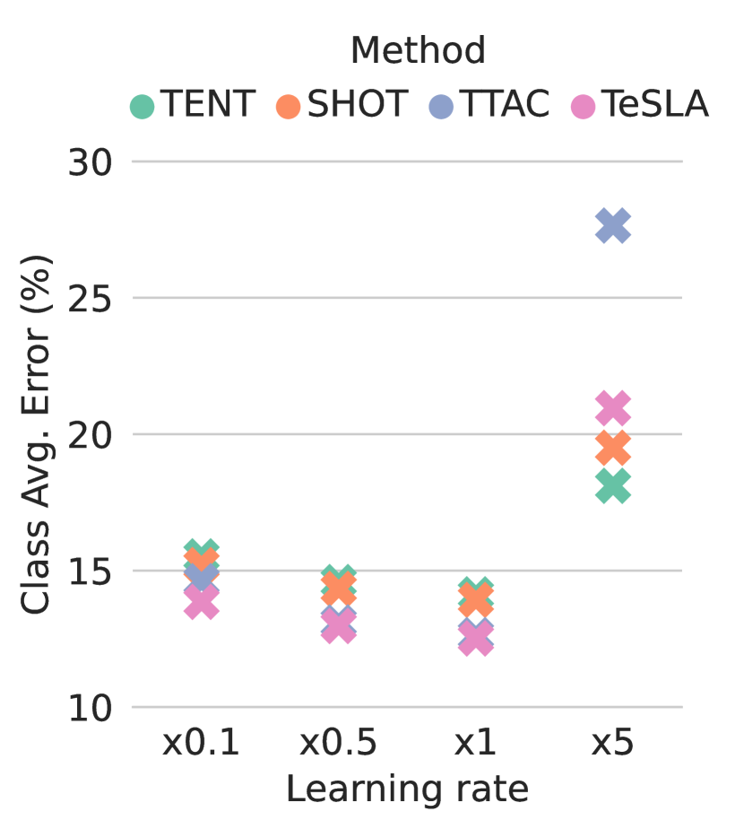
(b)

Figure E.7: Ablation study for the roles played by the (a) batch size $B$ and (b) the learning rate scale with respect to the default value. We report, for each baseline, the average error rate (in %) over four validation corruption sets of the CIFAR10-C under the N-O protocol.

Appendix F Additional Qualitative Results

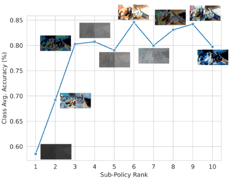
Figure F.1: Adversarial augmentation sanity check. We report the per-class average accuracy (%) of TeSLA’s student model on the VisDA-C augmented by the ten most adversarial sub-policies optimized by our automatic augmentation module.

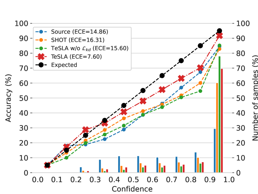
Figure F.2: Calibration performance comparison of TeSLA (with and without adversarial augmentations) against other baselines via a reliability diagram on the VisDA-C dataset for N-O protocol.

F.1 Sanity Check for Adversarial Augmentation

To assess the adversarial effect of the proposed automatic augmentations, we conduct a sanity check for the optimized sub-policies. in particular, in Fig. F.1, we rank the sub-policies optimized by our automatic augmentation module on the VisDA-C for N-M protocol after one epoch by decreasing the order of sampling probability. Then, we evaluate the performance of the student model on the test-test images from VisDA-C that are augmented using the above sub-policies. We observe that reducing the hardness level of sub-policies, the more the student model is accurate in recognizing the images. This is supported by the Pearson correlation of 0.7 between the sub-policy rank and the accuracy $(p=0.02)$, demonstrating our module’s capability to optimize and sample adversarial examples.

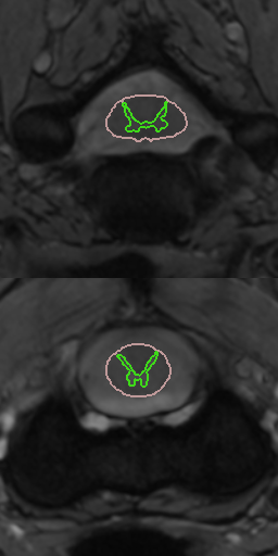
(a)

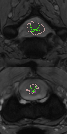
(b)

(c)

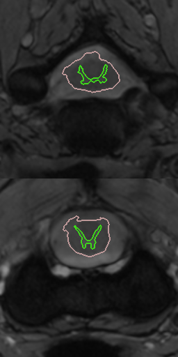
(d)

(e)

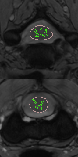
(f)

Figure F.3: Qualitative segmentation results of test-time adaptation methods trained on site 1 and tested on site 3 of the spinal cord dataset. From left to right: (a) Ground Truth, (b) Source Model, (c) BN[30], (d) TENT[45], (e) PL, and (f) TeSLA, respectively.

(a)

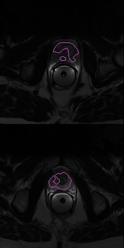
(b)

(c)

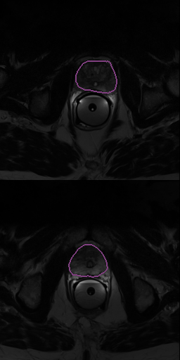
(d)

(e)

(f)

Figure F.4: Qualitative segmentation results of test-time adaptation method trained on site A and site B and tested on site F of the prostate dataset. From left to right: (a) Ground Truth, (b) Source Model, (c) BN[30], (d) TENT[45], (e) PL, and (f) TeSLA, respectively.

F.2 Uncertainty Evaluation

We evaluate the model reliability on the ViSDA-C classification adaptation task (N-O protocol). In Fig. F.2, we show the reliability diagram (dividing the probability range [0, 1.0] into ten bins) and report the expected calibration error (ECE) [31] for the Source model without adaptation, SHOT [26], and TeSLA with and without adversarial augmentations. The proposed TeSLA gives the lowest calibration error with an 8.71% improvement over SHOT. It is interesting to observe that the ECE of TeSLA without adversarial augmentations is on-par with the SHOT method. The adversarial augmentation module improves the TeSLA’s ECE by 8%, which shows the benefit of test-time adversarial augmentation on the model’s reliability.

F.3 Qualitative Segmentation Results

In Fig. F.3 and Fig. F.4, we show the qualitative segmentation results of TeSLA for test-time adaptation on the spinal cord and prostate MRI datasets and compare it with TENT[45], BN[30], and Pseudo Labeling (PL). Compared to other baselines, TeSLA outputs more accurate segmentation results closer to the provided ground truth.

References

- [1] Peshal Agarwal, Danda Pani Paudel, Jan-Nico Zaech, and Luc Van Gool. Unsupervised robust domain adaptation without source data. In Proceedings of the IEEE/CVF Winter Conference on Applications of Computer Vision, pages 2009–2018, 2022.
- [2] Arsenii Ashukha, Alexander Lyzhov, Dmitry Molchanov, and Dmitry Vetrov. Pitfalls of in-domain uncertainty estimation and ensembling in deep learning. In International Conference on Learning Representations, 2019.
- [3] Mathilde Caron, Hugo Touvron, Ishan Misra, Hervé Jégou, Julien Mairal, Piotr Bojanowski, and Armand Joulin. Emerging properties in self-supervised vision transformers. In Proceedings of the IEEE/CVF International Conference on Computer Vision, pages 9650–9660, 2021.
- [4] Dian Chen, Dequan Wang, Trevor Darrell, and Sayna Ebrahimi. Contrastive test-time adaptation. In Proceedings of the IEEE/CVF Conference on Computer Vision and Pattern Recognition, pages 295–305, 2022.
- [5] Liang-Chieh Chen, George Papandreou, Florian Schroff, and Hartwig Adam. Rethinking atrous convolution for semantic image segmentation. arXiv preprint arXiv:1706.05587, 2017.
- [6] Ting Chen, Simon Kornblith, Kevin Swersky, Mohammad Norouzi, and Geoffrey E Hinton. Big self-supervised models are strong semi-supervised learners. Advances in neural information processing systems, 33:22243–22255, 2020.
- [7] Marius Cordts, Mohamed Omran, Sebastian Ramos, Timo Rehfeld, Markus Enzweiler, Rodrigo Benenson, Uwe Franke, Stefan Roth, and Bernt Schiele. The cityscapes dataset for semantic urban scene understanding. In Proc. of the IEEE Conference on Computer Vision and Pattern Recognition (CVPR), 2016.
- [8] Ekin D Cubuk, Barret Zoph, Dandelion Mane, Vijay Vasudevan, and Quoc V Le. Autoaugment: Learning augmentation policies from data. arXiv preprint arXiv:1805.09501, 2018.
- [9] Ekin D Cubuk, Barret Zoph, Dandelion Mane, Vijay Vasudevan, and Quoc V Le. Autoaugment: Learning augmentation strategies from data. In Proceedings of the IEEE/CVF Conference on Computer Vision and Pattern Recognition, pages 113–123, 2019.
- [10] Ekin D Cubuk, Barret Zoph, Jonathon Shlens, and Quoc V Le. Randaugment: Practical automated data augmentation with a reduced search space. In Proceedings of the IEEE/CVF conference on computer vision and pattern recognition workshops, pages 702–703, 2020.
- [11] Alexey Dosovitskiy, Lucas Beyer, Alexander Kolesnikov, Dirk Weissenborn, Xiaohua Zhai, Thomas Unterthiner, Mostafa Dehghani, Matthias Minderer, Georg Heigold, Sylvain Gelly, Jakob Uszkoreit, and Neil Houlsby. An image is worth 16x16 words: Transformers for image recognition at scale. ICLR, 2021.
- [12] Cian Eastwood, Ian Mason, Christopher K. I. Williams, and Bernhard Schölkopf. Source-free adaptation to measurement shift via bottom-up feature restoration. In International Conference on Learning Representations, 2022.
- [13] Yaroslav Ganin and Victor Lempitsky. Unsupervised domain adaptation by backpropagation. In International conference on machine learning, pages 1180–1189. PMLR, 2015.
- [14] Alvaro Gomariz, Tiziano Portenier, César Nombela-Arrieta, and Orcun Goksel. Probabilistic spatial analysis in quantitative microscopy with uncertainty-aware cell detection using deep bayesian regression of density maps. arXiv preprint arXiv:2102.11865, 2021.
- [15] Kaiming He, Xiangyu Zhang, Shaoqing Ren, and Jian Sun. Deep residual learning for image recognition. In Proceedings of the IEEE conference on computer vision and pattern recognition, pages 770–778, 2016.
- [16] Dan Hendrycks and Thomas Dietterich. Benchmarking neural network robustness to common corruptions and perturbations. In International Conference on Learning Representations, 2019.
- [17] Judy Hoffman, Eric Tzeng, Taesung Park, Jun-Yan Zhu, Phillip Isola, Kate Saenko, Alexei Efros, and Trevor Darrell. Cycada: Cycle-consistent adversarial domain adaptation. In International conference on machine learning, pages 1989–1998. Pmlr, 2018.
- [18] Sergey Ioffe and Christian Szegedy. Batch normalization: Accelerating deep network training by reducing internal covariate shift. In International conference on machine learning, pages 448–456. PMLR, 2015.
- [19] Yusuke Iwasawa and Yutaka Matsuo. Test-time classifier adjustment module for model-agnostic domain generalization. Advances in Neural Information Processing Systems, 34:2427–2440, 2021.
- [20] Jakob Nikolas Kather, Johannes Krisam, Pornpimol Charoentong, Tom Luedde, Esther Herpel, Cleo-Aron Weis, Timo Gaiser, Alexander Marx, Nektarios A Valous, Dyke Ferber, et al. Predicting survival from colorectal cancer histology slides using deep learning: A retrospective multicenter study. PLoS medicine, 16(1):e1002730, 2019.
- [21] Jakob Nikolas Kather, Frank Gerrit Zöllner, Francesco Bianconi, Susanne M Melchers, Lothar R Schad, Timo Gaiser, Alexander Marx, and Cleo-Aron Weis. Collection of textures in colorectal cancer histology, May 2016.
- [22] Diederik P Kingma and Jimmy Ba. Adam: A method for stochastic optimization. arXiv preprint arXiv:1412.6980, 2014.
- [23] Jogendra Nath Kundu, Naveen Venkat, R Venkatesh Babu, et al. Universal source-free domain adaptation. In Proceedings of the IEEE/CVF Conference on Computer Vision and Pattern Recognition, pages 4544–4553, 2020.
- [24] Jogendra Nath Kundu, Naveen Venkat, Ambareesh Revanur, R Venkatesh Babu, et al. Towards inheritable models for open-set domain adaptation. In Proceedings of the IEEE/CVF Conference on Computer Vision and Pattern Recognition, pages 12376–12385, 2020.
- [25] Rui Li, Qianfen Jiao, Wenming Cao, Hau-San Wong, and Si Wu. Model adaptation: Unsupervised domain adaptation without source data. In Proceedings of the IEEE/CVF Conference on Computer Vision and Pattern Recognition, pages 9641–9650, 2020.
- [26] Jian Liang, Dapeng Hu, and Jiashi Feng. Do we really need to access the source data? source hypothesis transfer for unsupervised domain adaptation. In International Conference on Machine Learning, pages 6028–6039. PMLR, 2020.
- [27] Quande Liu, Qi Dou, Lequan Yu, and Pheng Ann Heng. Ms-net: Multi-site network for improving prostate segmentation with heterogeneous mri data. IEEE Transactions on Medical Imaging, 2020.
- [28] Yuejiang Liu, Parth Kothari, Bastien Germain van Delft, Baptiste Bellot-Gurlet, Taylor Mordan, and Alexandre Alahi. TTT++: When does self-supervised test-time training fail or thrive? In A. Beygelzimer, Y. Dauphin, P. Liang, and J. Wortman Vaughan, editors, Advances in Neural Information Processing Systems, 2021.
- [29] Alexander Lyzhov, Yuliya Molchanova, Arsenii Ashukha, Dmitry Molchanov, and Dmitry Vetrov. Greedy policy search: A simple baseline for learnable test-time augmentation. In Conference on Uncertainty in Artificial Intelligence, pages 1308–1317. PMLR, 2020.
- [30] Zachary Nado, Shreyas Padhy, D Sculley, Alexander D’Amour, Balaji Lakshminarayanan, and Jasper Snoek. Evaluating prediction-time batch normalization for robustness under covariate shift. arXiv preprint arXiv:2006.10963, 2020.
- [31] Alexandru Niculescu-Mizil and Rich Caruana. Predicting good probabilities with supervised learning. In Proceedings of the 22nd international conference on Machine learning, pages 625–632, 2005.
- [32] Xingchao Peng, Qinxun Bai, Xide Xia, Zijun Huang, Kate Saenko, and Bo Wang. Moment matching for multi-source domain adaptation. In Proceedings of the IEEE/CVF international conference on computer vision, pages 1406–1415, 2019.
- [33] Xingchao Peng, Ben Usman, Neela Kaushik, Judy Hoffman, Dequan Wang, and Kate Saenko. Visda: The visual domain adaptation challenge, 2017.
- [34] Ferran Prados, John Ashburner, Claudia Blaiotta, Tom Brosch, Julio Carballido-Gamio, Manuel Jorge Cardoso, Benjamin N Conrad, Esha Datta, Gergely Dávid, Benjamin De Leener, et al. Spinal cord grey matter segmentation challenge. Neuroimage, 152:312–329, 2017.
- [35] Zhen Qiu, Yifan Zhang, Hongbin Lin, Shuaicheng Niu, Yanxia Liu, Qing Du, and Mingkui Tan. Source-free domain adaptation via avatar prototype generation and adaptation. In International Joint Conference on Artificial Intelligence, 2021.
- [36] Stephan R. Richter, Vibhav Vineet, Stefan Roth, and Vladlen Koltun. Playing for data: Ground truth from computer games. In Bastian Leibe, Jiri Matas, Nicu Sebe, and Max Welling, editors, European Conference on Computer Vision (ECCV), volume 9906 of LNCS, pages 102–118. Springer International Publishing, 2016.
- [37] Olaf Ronneberger, Philipp Fischer, and Thomas Brox. U-net: Convolutional networks for biomedical image segmentation. In International Conference on Medical image computing and computer-assisted intervention, pages 234–241. Springer, 2015.
- [38] Mark Sandler, Andrew Howard, Menglong Zhu, Andrey Zhmoginov, and Liang-Chieh Chen. Mobilenetv2: Inverted residuals and linear bottlenecks. In Proceedings of the IEEE conference on computer vision and pattern recognition, pages 4510–4520, 2018.
- [39] Yongyi Su, Xun Xu, and Kui Jia. Revisiting realistic test-time training: Sequential inference and adaptation by anchored clustering. In Thirty-Sixth Conference on Neural Information Processing Systems, 2022.
- [40] Yu Sun, Xiaolong Wang, Zhuang Liu, John Miller, Alexei Efros, and Moritz Hardt. Test-time training with self-supervision for generalization under distribution shifts. In International conference on machine learning, pages 9229–9248. PMLR, 2020.
- [41] Antti Tarvainen and Harri Valpola. Mean teachers are better role models: Weight-averaged consistency targets improve semi-supervised deep learning results. Advances in neural information processing systems, 30, 2017.
- [42] Devavrat Tomar, Guillaume Vray, Jean-Philippe Thiran, and Behzad Bozorgtabar. OptTTA: Learnable test-time augmentation for source-free medical image segmentation under domain shift. In Medical Imaging with Deep Learning, 2022.
- [43] Laurens Van der Maaten and Geoffrey Hinton. Visualizing data using t-sne. Journal of machine learning research, 9(11), 2008.
- [44] Dequan Wang, Shaoteng Liu, Sayna Ebrahimi, Evan Shelhamer, and Trevor Darrell. On-target adaptation. arXiv preprint arXiv:2109.01087, 2021.
- [45] Dequan Wang, Evan Shelhamer, Shaoteng Liu, Bruno Olshausen, and Trevor Darrell. Tent: Fully test-time adaptation by entropy minimization. In International Conference on Learning Representations, 2021.
- [46] Guotai Wang, Wenqi Li, Michael Aertsen, Jan Deprest, Sébastien Ourselin, and Tom Vercauteren. Aleatoric uncertainty estimation with test-time augmentation for medical image segmentation with convolutional neural networks. Neurocomputing, 338:34–45, 2019.
- [47] Qin Wang, Olga Fink, Luc Van Gool, and Dengxin Dai. Continual test-time domain adaptation. In Proceedings of the IEEE/CVF Conference on Computer Vision and Pattern Recognition, pages 7201–7211, 2022.
- [48] Shiqi Yang, Yaxing Wang, Joost van de Weijer, Luis Herranz, and Shangling Jui. Casting a bait for offline and online source-free domain adaptation. arXiv preprint arXiv:2010.12427, 2020.
- [49] Shiqi Yang, Yaxing Wang, Joost van de Weijer, Luis Herranz, and Shangling Jui. Generalized source-free domain adaptation. In Proceedings of the IEEE/CVF International Conference on Computer Vision, pages 8978–8987, 2021.
- [50] Shiqi Yang, Yaxing Wang, Kai Wang, Shangling Jui, and Joost van de Weijer. Attracting and dispersing: A simple approach for source-free domain adaptation. arXiv preprint arXiv:2205.04183, 2022.
- [51] Yifan Zhang, Ying Wei, Qingyao Wu, Peilin Zhao, Shuaicheng Niu, Junzhou Huang, and Mingkui Tan. Collaborative unsupervised domain adaptation for medical image diagnosis. IEEE Transactions on Image Processing, 29:7834–7844, 2020.