Non–adiabatic effects lead to the breakdown of the semi–classical phonon picture

Abstract

Phonon properties of realistic materials are routinely calculated within the Density Functional Perturbation Theory (DFPT). This is a semi–classical approach where the atoms are assumed to oscillate along classical trajectories immersed in the electronic Kohn–Sham density, treated quantistically. In this work I demonstrate that, in metals, non–adiabatic effects induce a gap between the DFTP phonon frequencies and the fully quantistic solution of the phonon Dyson equation. A gap that increases with the phonon energy width reflecting the breakdown of the semi–classical DFPT description. The final message is that non–adiabatic phonon effects can be included only by using a fully quantistic approach.

I Introduction

The research on the physics induced or mediated by the lattice vibrations is crucial in many and disparate fields of modern solid–state physics: infrared spectroscopy, Raman, neutron-diffraction spectra, thermal transport are just a few of them Stefano Baroni (2001). Density Functional Theory (DFT) R.M.Dreizler and E.K.U.Gross (1990) and Density Functional Perturbation Theory(DFPT) Stefano Baroni (2001); Gonze (1995, 1997) have emerged as successful and widely used approaches to calculate the structural, electronic properties and also atomic dynamics in a fully ab–initio, framework. DFT and DFPT  are, nowadays, available in many public scientific codesGiannozzi et al. (2017); Gonze et al. (2009) and routinely used to calculate phonon frequencies and related properties.

Within DFT and DFPT  the atoms are treated classically and the atoms are assumed to move around the minimum of the Born–Oppenheimer surface Tavernelli (2015), with the electrons tightly bound to the atoms during their oscillations. In metallic materials the electronic excitations resonant with the phonon frequency cause a retardation between the electronic and atomic oscillations. This retardation is a non–adiabatic effect that induces, for example, the broadening of the phonon energy.

Indeed, from the experimental point of view it is well–known that the phonon peaks observed in the inelastic X–Ray scattering Shukla et al. (2003) or in the Raman spectra Ferrante et al. (2018) have an intrinsic energy width. This energy width is a natural concept within the Many–Body Perturbation Theory (MBPT) Stefanucci and van Leeuwen (2013); Marini (2023); Giustino (2017); van Leeuwen (2004); Marini et al. (2015); Stefanucci et al. (2023); Marini and Pavlyukh (2018), while the actual possibility to describe it in a semi–classical theory like DFPT  is still debated. Some works Lazzeri and Mauri (2006); Saitta et al. (2008); Calandra et al. (2010)have used perturbation theory to propose a frequency dependent extension of DFPT (FD–DFPT). This theory leads to the introduction of a frequency dependent and non–hermitian dynamical matrix whose eigenvalues, the phonons frequencies, are complex. FD–DFPT provides, thus, a picture conceptually equivalent to MBPT where non–adiabatic effects induce a renormalization and broadeding of the phonon energies. Moreover the enormous simplicity of FD–DFPT compared to the more involved MBPT approaches and its availability in many ab–initio  codes, has favored the application of the semi–classical DFPT  phonon concept beyond the adiabatic regime. The FD–DFPT has been applied to calculate, for examples: phonon widths Shukla et al. (2003); Lazzeri et al. (2005); Calandra et al. (2010), dynamical Kohn anomaliesPiscanec et al. (2004); Lazzeri and Mauri (2006), Raman spectra Saitta et al. (2008); Ferrante et al. (2018); Pisana (rint); Caudal et al. (2007) and non–adiabatic Born effective charges Dreyer et al. (2022); Binci et al. (2021).

These works have cemented the idea that a description based on a semi–classical representation of the atomic degrees of freedom is formally equivalent to the more involved Many–Body approach, with the difference that FD–DFPT relies on the change of the electronic density while MBPT requires to solve complicated equations written in terms of non–local phonon and electron Green’s functions.

In this work I mathematically demonstrate that, within non–adiabatic Density Functional Perturbation Theory, phonon widths are strictly zero. This implies that semi–classical atomic oscillations never decay in time, even when they are resonant with quantistic electron–hole pairs. I show that an infinite phonon lifetime is necessary to ensure that the dynamics conserves the total energy. The FD–DFPT approach will be demonstrated to correspond to the energy violating, and thus nonphysical, solution of the TD–DFPT equation. I conclude the work by comparing the TD–DFPT and MBPT phonon frequencies. I show that the two solutions diverge as the MBPT phonon width increases thus demonstrating that non–adiabatic effects can be described only by using a fully quantistic approach.

II The Hamiltonian and the problem

In order to describe non–adiabatic effects I rewrite DFPT in the time domain. I start from the perturbed DFT Hamiltonian written in second quantization:

$$\hat{H}=\sum_{i}\epsilon_{i}\hat{\rho}_{ii}+\sum_{\lambda}\biggl{[}\frac{\omega_{\lambda}}{2}\hat{p}_{\lambda}^{\dagger}\hat{p}_{\lambda}+\frac{\left(\omega_{\lambda}-C^{e-n}_{\lambda}\right)}{2}\hat{u}^{\dagger}_{\lambda}\hat{u}_{\lambda}\\ +\sum_{ij}g_{ji}^{\lambda}\Delta\hat{\rho}_{ij}\hat{u}_{\lambda}\biggr{]}+\sum_{ij}\Delta V^{Hxc}_{ji}\hat{\rho}_{ij}.$$ (1)

This Hamiltonian has been introduced by several authorsMarini (2023); Giustino (2017); van Leeuwen (2004); Marini et al. (2015); Stefanucci et al. (2023); Marini and Pavlyukh (2018) to discuss the connection between DFTP and MBPT. The procedure to derive Eq. (1) from the full DFT Hamiltonian is outlined in the Supplementary MaterialSection A.

Eq. (1) is written in terms of the single–particle DFT electronic and DFPT phononic energies, $\epsilon_{i}$ and $\omega_{\lambda}$. $\hat{\rho}_{ij}$ is the density matrix and $\hat{u}_{\lambda}$ and $\hat{p}_{\lambda}$ are the atomic displacement and momentum. $g^{\lambda}_{ji}$ is the bare electron–phonon potential that appears together with the variation of the the Hartree plus exchange–correlation potential (Hxc), $\Delta V^{Hxc}_{ji}$. $\hat{\rho}_{ij}$ is written in terms of the electronic creation and annihilation operators: $\hat{c}^{\dagger}_{i}/\hat{c}_{j}$ and $\Delta\hat{\rho}_{ij}=\hat{c}^{\dagger}_{i}\hat{c}_{j}-\left\langle\hat{c}^{\dagger}_{i}\hat{c}_{j}\right\rangle$.

In Eq. (1) $C^{e-n}_{\lambda}$ is the electron–nuclei (e–n) component of the reference DFPT phonon dynamical matrix. As it has been explained in Ref.Marini (2023); Marini et al. (2015); Stefanucci et al. (2023) this terms is already included in the $\omega_{\lambda}$ definition and needs to be removed in order to avoid double counting effects.

III Equations of motion: semi–classical trajectories and quantum fluctuations

The Hamiltonian $\hat{H}$ induces a time–dependent dynamics of all operators, electronic and atomic. These equations are derived in details in the Section B.

In the case of the atomic displacement operator we have

$$\hat{\mbox{$\mathcal{D}$}}_{\lambda}\left(t\right)\hat{u}_{\lambda}\left(t\right)=i\sum_{ij}g_{ji}^{\lambda}\int_{0}^{t}e^{i\Delta\epsilon_{ij}\left(t-\tau\right)}\\ \left[\underline{\hat{\rho}}\left(\tau\right),\underline{g}^{\lambda}\hat{u}_{\lambda}\left(\tau\right)+\underline{\Delta V}^{Hxc}\left[\rho\right]\right]_{ij}$$ (2)

with $\hat{\mbox{$\mathcal{D}$}}_{\lambda}\left(t\right)=\frac{1}{\omega_{\lambda}}\biggl{(}\frac{\mathrm{d}^{2}}{\mathrm{d}t^{2}}-\omega_{\lambda}\left(C^{e-n}_{\lambda}-\omega_{\lambda}\right)\biggr{)}$. $t=0$ is the initial time, underlined quantities are matrices in the single–particle basis, and $\Delta\epsilon_{ij}=\epsilon_{i}-\epsilon_{j}$.

The role of the $\underline{\Delta V}^{Hxc}$ potential is to dress the e–p interaction, as demonstrated in the Section C. In practice this means that we can remove $\underline{\Delta V}^{Hxc}$ from Eq. (2) and replace, in the commutator, $\underline{g}^{\lambda}$ with the screened and frequency dependent electron–phonon interaction, $\tilde{\underline{g}}^{\lambda}\left(\omega\right)=\underline{\underline{\epsilon}}^{-1}\left(\omega\right)\underline{g}^{\lambda}$, with $\underline{\underline{\epsilon}}^{-1}$ the dielectric tensor. For simplicity here we ignore the time dependence of $\underline{\underline{\epsilon}}^{-1}$ and assume $\tilde{\underline{g}}^{\lambda}\left(\omega\right)\approx\tilde{\underline{g}}^{\lambda}\left(\omega=0\right)$LK .

If we now take the average of both sides of Eq. (2) we note that it appears, in the r.h.s., the term $\left\langle\underline{\hat{\rho}}\left(t\right)\hat{u}_{\lambda}\left(t\right)\right\rangle$. This term prevents Eq. (2) to be written in terms of the electronic density matrix $\underline{\rho}\left(t\right)=\left\langle\underline{\hat{\rho}}\left(t\right)\right\rangle$ and atomic trajectory $u_{\lambda}\left(t\right)=\left\langle\hat{u}_{\lambda}\left(t\right)\right\rangle$ because

$$\left\langle\underline{\hat{\rho}}\left(t\right)\hat{u}_{\lambda}\left(t\right)\right\rangle=\underline{\rho}\left(t\right)u_{\lambda}\left(t\right)+\left\langle\underline{\Delta\hat{\rho}}\left(t\right)\Delta\hat{u}_{\lambda}\left(t\right)\right\rangle.$$ (3)

In Eq. (3) $\Delta{\hat{u}}\left(t\right)=\hat{u}\left(t\right)-u\left(t\right)$. The first term in Eq. (3) corresponds to the classical mean–field approximation and the second term represents the quantum corrections. From a physical point of view Eq. (3) makes clear that the mean–field term describes the trajectory ($\left\langle\hat{u}_{\lambda}\left(t\right)\right\rangle$) while the second term describes the fluctuations ($\left\langle\Delta\underline{\hat{\rho}}\left(t\right)\Delta\hat{u}_{\lambda}\left(t\right)\right\rangle$) around the classical trajectories. The term $\left\langle\Delta\underline{\hat{\rho}}\left(t\right)\Delta\hat{u}_{\lambda}\left(t\right)\right\rangle$ can be written in terms of the phonon propagator and self–energyMarini (2023); Giustino (2017); van Leeuwen (2004); Marini et al. (2015); Stefanucci et al. (2023); Marini and Pavlyukh (2018).

The semi–classical picture corresponds to assume $\left\langle\underline{\hat{\rho}}\left(t\right)\hat{u}_{\lambda}\left(t\right)\right\rangle\approx\underline{\rho}\left(t\right)u_{\lambda}\left(t\right)$. It is semi–classical because the atomic dynamics is described by a trajectory ($u_{\lambda}\left(t\right)$) while the electronic sub–system is treated fully quantistic.

As we are in the harmonic approximation we can further assume that the atomic displacements are tiny enough to approximate $\rho_{ij}\left(t\right)\sim f_{i}\delta_{ij}$, with $f_{i}$ the electronic occupations. It follows that

$$\hat{\mbox{$\mathcal{D}$}}_{\lambda}\left(t\right)u_{\lambda}\left(t\right)=-\int_{0}^{t}C_{\lambda}\left(t-\tau\right)u_{\lambda}\left(\tau\right)\mathrm{d}\tau,$$ (4a)

$$C_{\lambda}\left(t\right)=-\mathrm{i}\sum_{ij}\Delta f_{ij}g_{ji}^{\lambda}\tilde{g}^{\lambda}_{ij}e^{\mathrm{i}\Delta\epsilon_{ij}t},$$ (4b)

with $\Delta f_{ij}=f_{i}-f_{j}$. Eq. (4) is the Time–Dependent DFPT equation of motion whose solution is defined in terms of the the boundary conditions at $t=0$. Here we define $u_{\lambda}\left(0\right)=u^{0}_{\lambda}$ and $\frac{\mathrm{d}}{\mathrm{d}t}u_{\lambda}\left(0\right)=v^{0}_{\lambda}$.

IV The adiabatic limit: DFPT

The adiabatic DFPT can now be obtained from Eq. (4) by assuming $\Delta\epsilon_{ij}\gg\omega_{\lambda}$. This implies that during the rapid electronic oscillations the atoms do not move and, in the r.h.s. of Eq. (4), $u_{\lambda}\left(\tau\right)\approx u_{\lambda}\left(t\right)$. In this way the r.h.s. of Eq. (4) can be calculated analytically to give

$$\hat{\mbox{$\mathcal{D}$}}_{\lambda}\left(t\right)u_{\lambda}\left(t\right)=-C^{st}_{\lambda}u_{\lambda}\left(t\right)+\sum_{ij}\frac{\Delta f_{ij}g_{ji}^{\lambda}\tilde{g}^{\lambda}_{ij}}{\Delta\epsilon_{ij}}e^{\mathrm{i}\Delta\epsilon_{ij}t},$$ (5)

with $C^{st}_{\lambda}=\sum_{ij}\frac{\Delta f_{ij}g_{ji}^{\lambda}\tilde{g}^{\lambda}_{ij}}{\Delta\epsilon_{ij}}$. As $\Delta\epsilon_{ij}\gg\omega_{\lambda}$ Eq. (5) can be time integrated over an electronic period much shorter than the phonon period, where the integral of the last term in the r.h.s. of Eq. (5) vanishes. This means that, within the adiabatic approximation, $\omega_{\lambda}$ represents the frequency of the slow oscillation of the solution of Eq. (5) when $C^{e-n}_{\lambda}=C^{st}_{\lambda}$ confirming that DFPT corresponds to the take the static (adiabatic) limit of the TD–DFPT kernel.

V TD–DFPT

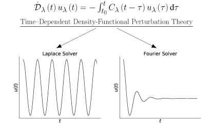
Figure 1: The two solvers (Laplace and Fourier) of the TD–DFPT equation, Eq. (4), are schematically compared. $u\left(t\right)$ is the atomic displacement function. While the Laplace approach leads to persistent oscillations the Fourier solution produces an artificial damping that violates the energy conservation. The Fourier solution corresponds to the frequency–dependent DFPT proposed by Ref.Lazzeri and Mauri (2006); Saitta et al. (2008); Calandra et al. (2010) and currently implemented in many ab–initio  DFPT codes publicly released.

In metals the adiabatic ansatz breaks down as the metallic electronic transition and atomic oscillation energies are similar, $\Delta\epsilon_{ij}\sim\omega_{\lambda}$. Therefore non–adiabatic effects appear and, in Eq. (4), it is not possible to assume $u_{\lambda}\left(\tau\right)\sim u_{\lambda}\left(t\right)$.

The TD–DFPT phonon frequencies correspond, therefore, to the solution of Eq. (4). This is a second–order Volterra linear integro–differential equation Wazwaz (2011) with a separable kernel ($e^{\mathrm{i}\Delta\epsilon_{ij}\left(t-\tau\right)}$). The Volterra equations are the subject of an intense mathematical research activity as they appear in many physical contexts like, for example, the dynamics of viscoelastic materials Alabau-Boussouira et al. (2008) or applications of physical engineering Zakęś and Śniady (2016).

A crucial property of Eq. (4) is that, being based on the mean–field approximation, leads to an energy conserving dynamics. This means that if $E=\left\langle\hat{H}\right\rangle$ the solution of Eq. (4) must lead to a time independent and constant $E$.

To solve Eq. (4) I use the Laplace transformation, which is commonly used to solve the free quantum harmonic oscillator equation Wazwaz (2011); Boas (2015)

$$f\left(z\right)=\mbox{$\mathcal{L}$}[f]\left(z\right)=\int_{0}^{\infty}e^{-zt}f\left(t\right)d\,t.$$ (6)

When $z=-\mathrm{i}\omega$ Eq. (6) reduces to the Fourier transformation. We consider here both transformations because, as it will demonstrated shortly, the use of the Fourier will lead to the FD–DFPT theory proposed in  Lazzeri and Mauri (2006); Saitta et al. (2008); Calandra et al. (2010), and widely used in the literature, which predicts the non–adiabatic effects to induce a finite phonon energy indetermination, corresponding to complex phonon frequencies.

We now proceed to apply Eq. (6) to Eq. (4) and we note that, when $z=-\mathrm{i}\omega$ (Fourier), $\mbox{$\mathcal{L}$}[\hat{\mbox{$\mathcal{D}$}}_{\lambda}u_{\lambda}]\left(-\mathrm{i}\omega\right)$ is well defined only and only if $u_{\lambda}\left(t=\infty\right)=0$. The mathematical reason is that, in order to transform the time differential operator, we need to use the integration by parts method which requires the integrand of Eq. (6) to vanish at $t=\infty$ (Section D). This means, in practice, that the Fourier case can be used only by applying a tiny exponential prefactor, $e^{-\eta t}$, and send $\eta$ to zero at the end of derivation. We thus consider $f\left(z\right)$ and $f\left(-\mathrm{i}\omega+\eta\right)$, with $\eta\rightarrow 0$.

By using Eq. (6) it follows that

$$u_{\lambda}\left(z\right)=\frac{zu_{\lambda}^{0}+v_{\lambda}^{0}}{z^{2}+\omega^{2}_{\lambda}+\omega_{\lambda}\Delta C_{\lambda}\left(z\right)},$$ (7a)

with $$\Delta C_{\lambda}\left(z\right)=C_{\lambda}\left(z\right)-C_{\lambda}^{e-n}$$ and

$$C_{\lambda}\left(z\right)=-\mathrm{i}\sum_{ij}g_{ji}^{\lambda}\tilde{g}_{ij}^{\lambda}\frac{\Delta f_{ij}}{z-\mathrm{i}\Delta\epsilon_{ij}}.$$ (7b)

$u_{\lambda}\left(t\right)$ can be analytically obtained from $u_{\lambda}\left(z\right)$ by using the Bromwhich integral Boas (2015) method that involves a complex plane integral of $u_{\lambda}\left(z\right)$. From Eq. (7) it follows that the solution of Eq. (4) is equivalent to find the poles of $u_{\lambda}\left(z\right)$. In the Laplace case this corresponds to find the zeros of

$$z^{2}+\omega^{2}_{\lambda}+\omega_{\lambda}\Delta C_{\lambda}\left(z\right)=0,$$ (8a)

while in the Fourier case we have

$$-\omega^{2}+\omega^{2}_{\lambda}+\omega_{\lambda}\lim_{\eta\rightarrow 0}\Delta C_{\lambda}\left(-\mathrm{i}\omega+\eta\right)=0.$$ (8b)

We now remind that $\lim_{\eta\rightarrow 0}\frac{1}{\omega+\Delta\epsilon_{ij}+\mathrm{i}\eta}=\mbox{$\mathcal{P}$}\left[\frac{1}{\omega+\Delta\epsilon_{ij}}\right]-\mathrm{i}\pi\delta\left(\omega+\Delta\epsilon_{ij}\right)$, with $\mathcal{P}$ the Cauchy principal and real value. Therefore it follows that

$$\lim_{\eta\rightarrow 0}\Delta C_{\lambda}\left(-\mathrm{i}\omega+\eta\right)=\mbox{$\mathcal{P}$}\left[\Delta C_{\lambda}\left(-\mathrm{i}\omega\right)\right]+\mathrm{i}\Gamma_{\lambda}\left(\omega\right),$$ (9)

with

$$\Gamma_{\lambda}\left(\omega\right)=-\pi\sum_{ij}g_{ji}^{\lambda}\tilde{g}_{ij}^{\lambda}\Delta f_{ij}\delta\left(\omega+\Delta\epsilon_{ij}\right).$$ (10)

Eq. (9) implies that the poles defined by Eq.(8b) are complex. In the Laplace case, instead, we observe that by definition $C_{\lambda}^{e-n}\in\mathbb{R}$ and $\Delta C_{\lambda}\left(z\right)=\mbox{$\mathcal{P}$}\left[C_{\lambda}\left(z\right)\right]$. It follows that the Laplace solution leads to imaginary poles corresponding to real frequencies.

If we call the zeros of Eq.(8a) $\Omega^{CM}_{\lambda}$ we thus finally get

$$u_{\lambda}\left(t\right)=\sum_{s=\pm}\begin{cases}e^{\mathrm{i}s\Omega^{CM}_{\lambda}t}u_{\lambda s}&Laplace\\ e^{\mathrm{i}s{\rm Re}\left[\Omega^{CM}_{\lambda}\right]t}e^{-\mathrm{i}{\rm Im}\left[\Omega^{CM}_{\lambda}\right]t}u_{\lambda s}&Fourier\end{cases}$$ (11)

In Eq. (11) the $u_{\lambda s}$ constants are defined in terms of the initial position and velocity, $u_{\lambda}^{0}$ and $v_{\lambda}^{0}$. Eq. (11) demonstrates that $u_{\lambda}\left(t\rightarrow\infty\right)=0$ only when the TD–DFPT master equation is solved by using the Fourier transformation. In this case we recover the FD–DFPT Lazzeri and Mauri (2006); Saitta et al. (2008); Calandra et al. (2010).

FD–DFPT is obtained, therefore, when $u_{\lambda}\left(t\right)$ and the kernel $C_{\lambda}\left(t\right)$ are artificially dumped (via $e^{-\eta t}$) from the beginning. Even if $\eta\rightarrow 0$ at the end of the derivation the solution remains damped and produces an artificial decay of the oscillations. This decay is nonphysical as it makes $\left\langle H\right\rangle$ time–dependent while the Hamiltonian, Eq. (1) is not time–dependent. More importantly, as we are in the linear regime and $f_{i}$ is time–independent, decaying atomic oscillations lead to a decaying total energy. This is in contrast with the fact that within the mean–field approximation the energy is conserved. The Laplace solution instead corresponds to persistent oscillating solutions which represent a set of un–damped independent harmonic oscillators whose total energy is constant and conserved.

VI MBPT phonons

Now the natural question is what is the impact om the phonon energies of the absence, in the semi–classical TD–DFPT case, of any energy indetermination. Are the TD–DFPT phonon energies still reliable?

In order to answer this question we need to estimate the impact of the phonon line–width on its energy. To do this we use the MBPT approach where the phonon frequencies are defined as solution of the Dyson equation for the phonon Green’s function, $D_{\lambda}\left(t,t^{\prime}\right)=-\mathrm{i}\left\langle\mbox{$\mathcal{T}$}\{\Delta\hat{u}_{\lambda}\left(t\right)\Delta\hat{u}\left(t^{\prime}\right)\}\right\rangle$Stefanucci and van Leeuwen (2013). The poles of the Fourier transformed $D_{\lambda}\left(-\mathrm{i}\omega\right)$ (using the convention defined by Eq. (6)) with respect to $\left(t-t^{\prime}\right)$ are the MBPT phonon energies, $\Omega^{QM}_{\lambda}+\mathrm{i}\gamma^{QM}_{\lambda}$. Here I use the Quantum Mechanics (QM) label for MBPT quantities. Those poles are solution of the fixed point equation

$$\omega^{2}-\omega^{2}_{\lambda}+\omega_{\lambda}C^{e-n}_{\lambda}-\omega_{\lambda}\Pi_{\lambda}\left(-\mathrm{i}\omega\right)=0.$$ (12)

The usual interpretation is that while $\Omega^{QM}_{\lambda}$ is the renormalized phonon energy, $\gamma^{QM}_{\lambda}$ defines its energy indetermination.

In Eq. (12) $\Pi_{\lambda}\left(-\mathrm{i}\omega\right)$ is the Fourier transformed of the Phonon self-energy:

$$\Pi_{\lambda}\left(-\mathrm{i}\omega\right)=\sum_{ij}g_{ji}^{\lambda}\tilde{g}_{ij}^{\lambda}\frac{\Delta f_{ij}}{\omega+\Delta\epsilon_{ij}+\mathrm{i}\xi}.$$ (13)

In Eq. (13) $\xi$ is a tiny positive number that appears because of the adiabatic switching on of the interaction. Thanks to the Gell–Mann&Low theorem Alexander L. Fetter (1971) it is possible to send $\xi\rightarrow 0$. Thanks to this basic theorem of MBPT $\Pi_{\lambda}\left(-\mathrm{i}\omega\right)$ acquires a finite imaginary part and, consequently, provides the phonon with a finite energy indetermination.

The formally analogy of Eq. (13) and Eq.(8b) has instilled the idea that non–adiabatic effects can be described by DFPT with the same accuracy of MBPT. From a physical point of view this would mean that a fully quantistic approach is equivalent to treat the atoms semi–classically. Here, instead, I demonstrated that this not true and the semi–classical TD–DFPT approach has no access to the phonon energy indetermination.

VII TD–DFPT versus MBPT and the breakdown of the semi–classical phonon picture

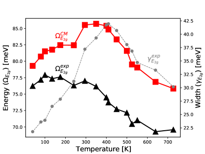
Figure 2: MgB₂ experimental width ($\gamma_{E_{2g}}^{exp}$, gray line, circles) and energy ($\Omega_{E_{2g}}^{exp}$, black line, triangles) of the E_2g phonon mode as a function of the temperaturePonosov and Streltsov (2017) compared with the semi–classical TD–DFPT phonon energies ($\Omega_{E_{2g}}^{CM}$, red line, boxes). MgB₂ is well known to manifest strong non–adiabatic effects that result in a phonon width that, at room temperature, is almost half of the phonon energy. This very large width causes an equally large (15%) TD–DFPT overestimation of the phonon frequency.

In order to estimate the impact of the difference $\Omega^{CM}_{\lambda}-\Omega^{QM}_{\lambda}$ in realistic materials let’s compare the solution of Eq. (12) with Eq.(8a) in MgB₂, a paradigmatic material characterized by very large non–adiabatic effects Choi et al. (2002). We can safely assume that ${\rm Re}\left[\Pi_{\lambda}\left(-\mathrm{i}\omega\right)\right]\sim\mbox{$\mathcal{P}$}\left(C_{\lambda}\left(-\mathrm{i}\omega\right)\right)$. It follows that we can rewrite the real part of Eq. (12) as

$$\left(\Omega^{QM}_{\lambda}\right)^{2}+\left(\gamma^{QM}_{\lambda}\right)^{2}=\left(\Omega^{CM}_{\lambda}\right)^{2}.$$ (14)

Eq. (14) is demonstrated analytically in Section F, and it represents another result of this work. It provides an easy recipe to estimate the deviation of the TD–DFPT phonon energy from the MBPT result when the phonon acquires a finite width. First of all, we see that $\Omega^{CM}_{\lambda}>\Omega^{QM}_{\lambda}$ which means that the semi–classical phonon frequency is always larger than the MBPT one. More importantly we can apply Eq. (14) to any material whose experimental phonon energies and widths have been either calculated or measured experimentally.

Indeed if we suppose to use the exact MBPT self–energy, then $\Omega^{QM}_{\lambda}$ ($\gamma^{QM}_{\lambda}$) is, by definition, equal to the experimental frequency (width). So we can use a slightly modified version of Eq. (14):

$$\Omega^{CM}_{\lambda}=\sqrt{\left(\Omega^{exp}_{\lambda}\right)^{2}+\left(\gamma^{exp}_{\lambda}\right)^{2}}.$$ (15)

In the case of MgB₂ we can apply Eq. (15) to the $E_{2g}$ mode measured via Raman scattering by Ponoso and Streltsov in Ref.Ponosov and Streltsov (2017), whose energy (black line) and width (gray line) are reported as a function of the temperature in Fig.2. We notice that at $T\sim 410$K $\gamma^{exp}_{E_{2g}}$ reaches its maximum, $41.9$ meV, that corresponds to $\sim$57% of the frequency ($73.7$ meV). In this case Eq. (15) gives $\Omega^{CM}_{\lambda}=84.83$ meV, which corresponds to a 15% overestimation of the experimental value.

In Ref.Saitta et al. (2008) the DFPT approach has been applied to several conventional and layered metals finding deviations of the experimental phonon frequencies from the adiabatic DFTP results ranging from $\sim 4.5$% (CaC₆ at 300K) to $\sim 24.5$%(KC₈). These deviations are of the same order of magnitude of the $\Omega^{CM}_{\lambda}-\Omega^{QM}_{\lambda}$. This confirms that non–adiabatic effects cannot be described by TD–DFPT and impose the use of a fully quantistic approach.

VIII Conclusions

In this work I propose a time–dependent formulation of Density Functional Perturbation Theory that extends the semi–classical phonon concept to the non–adiabatic regime. By solving exactly the integro–differential equation which governs the atomic oscillations dynamics I have demonstrated that phonon energies are purely real and that a semi–classical description has no access to the phonon energy indetermination.

By comparing the TD–DFPT solution with the quasi–phonon Many–Body picture I derive a simple equation that allows to estimate, even experimentally, the impact of the semi–classical phonon assumption. This method is applied to MgB₂ showing large ($15$% of the bare phonon frequency) overestimation of the experimental phonon energy when using TD–DFPT. This overestimation reflects the breakdown of the semi–classical picture. The final results is that the semi–classical DFTP phonon approach cannot describe non–adiabatic effects. In this case a fully quantistic scheme is needed. The present results open several questions in many different fields of physics and call for further research on the impact of non–adiabatic effects on the atomic dynamics within and beyond the harmonic approximation.

IX Acknowledgments

A.M. would like to acknowledge F. Paleari, G. Stefanucci and E. Perfetto for helpful discussions. A.M. acknowledges the funding received from the European Union projects: MaX Materials design at the eXascale H2020-INFRAEDI-2018-2020/H2020-INFRAEDI-2018-1, Grant agreement n. 824143; Nanoscience Foundries and Fine Analysis – Europe | PILOT H2020-INFRAIA-03-2020, Grant agreement n. 101007417; PRIN: Progetti di Ricerca di rilevante interesse Nazionale Bando 2020, Prot. 2020JZ5N9M.

Appendix A The initial Hamiltonian

The perturbed Density Functional Theory (DFT) Hamiltonian has been introduced by several authors Marini (2023); Giustino (2017); van Leeuwen (2004); Marini et al. (2015); Stefanucci et al. (2023); Marini and Pavlyukh (2018). I take as reference eq. 24 of Ref.Marini (2023):

$$\widehat{H}=\sum_{i}\epsilon_{i}\hat{c}^{\dagger}_{i}\hat{c}_{i}+\widehat{H}_{e-e}+\\ +\sum_{\lambda}\biggl{[}\frac{\omega_{\lambda}}{2}\left(\hat{u}^{\dagger}_{\lambda}\hat{u}_{\lambda}+\hat{p}^{\dagger}_{\lambda}\hat{p}_{\lambda}\right)+\\ +\left(\hat{\mbox{$\mathcal{L}$}}_{\lambda}+\sum_{\mu}\hat{\mbox{$\mathcal{Q}$}}_{\mu\lambda}\hat{\phi}_{+\mu}\right)\hat{\phi}_{+\lambda}\biggr{]}$$ (16)

where $\hat{\mbox{$\mathcal{L}$}}_{\lambda}$, $\hat{\mbox{$\mathcal{Q}$}}_{\lambda\mu}$ are defined in eq. 25 of Ref.Marini (2023) .

As I am working within DFT the electron–electron interaction is replaced by the exact mean–field exchange–correlation potential, $\underline{\Delta V}^{Hxc}$.

In the present context I assume that the equilibrium positions the atoms are oscillating around are well described by the adiabatic DFPT, with negligible non–adiabatic corrections. Thanks to this assumption

$$\hat{\mbox{$\mathcal{L}$}}_{\lambda}=\sum_{ij}g_{ji}^{\lambda}\Delta\hat{\rho}_{ij}.$$ (17)

Similarly I neglect second–order terms in Eq. (16) in $\hat{\phi}_{s\lambda}$ which induces non–harmonic corrections to the atomic equation of motion. Thanks to this approximation

$$\hat{\mbox{$\mathcal{Q}$}}_{\lambda\mu}=-\frac{1}{2}C^{e-n}_{\lambda\mu}.$$ (18)

I further assume $C^{e-n}_{\lambda\mu}\sim C^{e-n}_{\lambda\mu}\delta_{\lambda\mu}$.

By using Eqs. (17)–(18) in Eq. (16) we obtain Eq.(2) of the body of this work.

The notation used in Eq. (16) is very general. The $i$ label can represent any one–body quantum number. If we consider, for example, the electronic momentum ${\mathbf{k}}$ (bold symbols are vectors) Eq. (16) turns into

$$\widehat{H}=\sum_{{\mathbf{k}}}\epsilon_{{\mathbf{k}}}\hat{c}^{\dagger}_{{\mathbf{k}}}\hat{c}_{{\mathbf{k}}}+\sum_{\lambda{\mathbf{q}}}\biggl{[}\frac{\omega_{{\mathbf{q}}\lambda}}{2}\left(\hat{u}^{\dagger}_{{\mathbf{q}}\lambda}\hat{u}_{{\mathbf{q}}\lambda}+\hat{p}^{\dagger}_{{\mathbf{q}}\lambda}\hat{p}_{{\mathbf{q}}\lambda}\right)+\\ +\sum_{{\mathbf{k}}}\biggl{(}g_{{\mathbf{q}}}^{\lambda}\hat{u}_{{\mathbf{q}}\lambda}+V^{Hxc}_{\mathbf{q}}\biggr{)}\hat{c}^{\dagger}_{{\mathbf{k}}}\hat{c}_{{\mathbf{k}}-{\mathbf{q}}}\biggr{]}.$$ (19)

From Eq. (19), the very same procedure described in the main text leads to

$$C_{{\mathbf{q}}\lambda}\left(z\right)=-\mathrm{i}g_{{\mathbf{q}}}^{\lambda}\tilde{g}_{-{\mathbf{q}}}^{\lambda}\sum_{\mathbf{k}}\frac{f_{{\mathbf{k}}}-f_{{\mathbf{k}}+{\mathbf{q}}}}{z-\mathrm{i}\left(\epsilon_{{\mathbf{k}}}-\epsilon_{{\mathbf{k}}+{\mathbf{q}}}\right)}.$$ (20)

Eq. (20) is equivalent to Eq.(145) of Ref.Giustino (2017), for example. In a similar way band indexes can be added. The derivation of the main text will not depend on the specific notation used as it is completely agnostic of the underling one–body representation.

Appendix B Equations of motion for the electronic and bosonic operators

The Hamiltonian defined in Eq.(2) of the main text induces a dynamics of all operators, electronic and atomic. These equations have been recently reviewed in Ref.Marini (2023); Marini et al. (2015); Stefanucci et al. (2023). The second–order time derivative of the displacement is

$$\frac{\mathrm{d}^{2}}{\mathrm{d}t^{2}}\hat{u}_{\lambda}\left(t\right)=\omega_{\lambda}\left(\Pi^{st}_{\lambda}-\omega_{\lambda}\right)\hat{u}_{\lambda}\left(t\right)-\omega_{\lambda}\sum_{ij}g_{ji}^{\lambda}\Delta\hat{\rho}_{ij}\left(t\right),$$ (21)

while the equation of motion for the density matrix is

$$i\frac{\mathrm{d}}{\mathrm{d}t}\hat{\rho}_{ij}\left(t\right)=-\Delta\epsilon_{ij}\hat{\rho}_{ij}\left(t\right)\\ +\sum_{\lambda}\left[\underline{\hat{\rho}}\left(t\right),\underline{g}^{\lambda}\hat{u}_{\lambda}\left(t\right)\right]_{ij}+\left[\underline{\hat{\rho}}\left(t\right),\Delta\underline{V}^{Hxc}\left[\rho\left(t\right)\right]\right]_{ij}$$ (22)

Eqs. (21)–(22) completely solve the Many–Body problem and produce the equations governing the classical atomic motion as an approximation as explained in main text.

Appendix C Electron–phonon interaction dynamical dressing

The role of $V^{Hxc}$ in Eq. (22) is to screen the electron–phonon interaction $g^{\lambda}_{ji}$. In order to see it we observe that Marques et al. (2012)

$$\underline{\Delta V}^{Hxc}\left[\rho\right]\left(t\right)=\int\mathrm{d}\tau\,t^{\prime}\underline{\underline{f}}^{Hxc}\left(t-\tau\right)\delta\underline{\rho}\left(\tau\right)=\\ \sum_{\lambda}\int\mathrm{d}\tau\,t^{\prime}\underline{\underline{f}}^{Hxc}\left(t-\tau\right)\underline{\underline{\chi}}\left(\tau-t^{\prime}\right)\underline{g}^{\lambda}u_{\lambda}\left(t^{\prime}\right),$$ (23)

with $\underline{\underline{\chi}}$ the tensorial reducible response function and $\underline{\underline{f}}^{Hxc}$ the Hartree plus exchange–correlation kernel, defined as $\frac{\delta\underline{V}^{Hxc}\left[\rho\right]\left(t\right)}{\delta\underline{\rho}\left(t^{\prime}\right)}$. The single underlined quantities are matrices ($\underline{M}_{ij}$) while the doubly underlined are tensors ($\underline{\underline{M}}_{\begin{subarray}{c}ij\\ kl\end{subarray}}$) in the electron–hole pairs space. If we now plug Eq. (23) in Eq. (22) and take the average of both terms we get

$$\underline{g}^{\lambda}u_{\lambda}\left(t\right)+\underline{\Delta V}^{Hxc}\left[\rho\left(t\right)\right]=\sum_{\mu}\int\mathrm{d}t^{\prime}\biggl{[}\underline{\underline{\delta}}\delta_{\lambda\mu}\delta\left(t-t^{\prime}\right)+\\ +\int d\tau\underline{\underline{f}}^{Hxc}\left(t-\tau\right)\underline{\underline{\chi}}\left(\tau-t^{\prime}\right)\biggr{]}\underline{g}^{\mu}u_{\mu}\left(t^{\prime}\right)\sim\\ \int\mathrm{d}t^{\prime}\underline{\underline{\varepsilon}}^{-1}\left(t-t^{\prime}\right)\underline{g}^{\lambda}u_{\lambda}\left(t^{\prime}\right).$$ (24)

In Eq. (24) it appears the TD–DFT inverse test–electron Marini et al. (2015) dielectric matrix, $\underline{\underline{\varepsilon}}^{-1}\left(t-t^{\prime}\right)$, and I have neglected the $\lambda\neq\mu$ terms.

If we now use Eq. (24) in Eq. (22) we get

$$\Delta\underline{\rho}\left(t\right)=\int\mathrm{d}t^{\prime}\underline{\underline{\chi}}\left(t-t^{\prime}\right)\underline{g}^{\lambda}u_{\lambda}\left(t^{\prime}\right),$$ (25)

that corresponds to the TD–DFT Kubo equation. If we now use the Källén–Lehmann spectral representation of $\underline{\underline{\chi}}\left(t-t^{\prime}\right)$ Alexander L. Fetter (1971) we can expand Eq. (25) over the poles ($E_{I}$) and residuals ($\underline{\underline{\chi}}^{I}$) of $\underline{\underline{\chi}}$:

$$\rho_{ij}\left(t\right)=\sum_{I}\left[\underline{\underline{\chi}}^{I}\underline{g}^{\lambda}\right]_{ij}\int\mathrm{d}t^{\prime}e^{\mathrm{i}E_{I}\left(t-t^{\prime}\right)}u_{\lambda}\left(t^{\prime}\right),$$ (26)

From Eq. (26) it follows that the effect of the time–dependent exchange–correlation DFT potential is to replace the independent particle energies with the poles of the full TD–DFT response function. Again, Eq. (26) does not lead to any change in the main derivations of the work where, for simplicity, I use the static screening approximation and write

$$\rho_{ij}\left(t\right)\approx\tilde{g}^{\lambda}_{ij}\int\mathrm{d}t^{\prime}e^{\mathrm{i}\Delta\epsilon_{ij}\left(t-t^{\prime}\right)}u_{\lambda}\left(t^{\prime}\right),$$ (27)

with $\underline{\tilde{g}}^{\lambda}\sim\underline{\underline{\varepsilon}}^{-1}\left(\omega=0\right)\underline{g}^{\lambda}$.

Appendix D On the Laplace and Fourier transformations of the differential operator

The Laplace and Fourier transformations are, apparently, very similar:

$$g^{f}\left(\omega\right)=\int_{0}^{\infty}e^{\mathrm{i}\omega t}g\left(t\right)\mathrm{d}t,$$ (28a)

$$g^{l}\left(\omega\right)=\int_{0}^{\infty}e^{-\omega t}g\left(t\right)\mathrm{d}t.$$ (28b)

In Eq. (28) I have assumed $g\left(t\right)=0$ when $t<0$, which is the case of a classical pendulous displaced from the equilibrium position at $t=0$.

The Fourier transformation is not listed among the solvers of the integro–differential Volterra equationWazwaz (2011); Boas (2015) and the reason is simple. If we apply Eq.(28a) to the differential operator ($\frac{\mathrm{d}^{2}}{\mathrm{d}t^{2}}$) we get

$$\int_{0}^{\infty}e^{\mathrm{i}\omega t}\frac{\mathrm{d}^{2}u_{\lambda}\left(t\right)}{\mathrm{d}t^{2}}\mathrm{d}t=\left.e^{\mathrm{i}\omega t}\frac{\mathrm{d}u_{\lambda}\left(t\right)}{\mathrm{d}t}\right|_{0}^{\infty}\\ -\mathrm{i}\omega\left[\left.e^{\mathrm{i}\omega t}u_{\lambda}\left(t\right)\right|_{0}^{\infty}-\mathrm{i}\omega u_{\lambda}^{f}\left(\omega\right)\right],$$ (29)

with $u_{\lambda}^{f}\left(\omega\right)$ the Fourier transformation of $u\left(t\right)$. From Eq. (29) it is evident that in order for the differential operator to be Fourier transformable we do need to impose the condition $\left.\frac{\mathrm{d}u_{\lambda}\left(t\right)}{\mathrm{d}t}\right|_{t=\infty}=u_{\lambda}\left(t=\infty\right)=0$. Therefore the Fourier transformation can be used if and only if it is assumed from the beginning that the solution will decay in time.

This a peculiar property of the Volterra equation: if we start from the sub–space of function that decay for $t\rightarrow\infty$ the solution will decay as well even if at the end of the derivation we extend the initial sub–space of functions to the entire space.

Appendix E Regularization of the Laplace transformation of the time–dependent DFPT kernel

We now notice that $C_{\lambda}\left(\mathrm{i}\Delta\epsilon_{km}\right)=\infty$ for any $\Delta\epsilon_{km}$. This means that $u_{\lambda}\left(z\right)$ is ill defined when $z$ approaches the electron–hole energies. However let’s rewrite $C_{\lambda}\left(\omega\right)$ as

$$C_{\lambda}\left(\omega\right)=\left(-\mathrm{i}\right)\frac{\sum_{J}R^{\lambda}_{J}\prod_{I\neq J}\left(\omega-\mathrm{i}\Delta\epsilon_{I}\right)}{\prod_{I}\left(\omega-\mathrm{i}\Delta\epsilon_{I}\right)},$$ (30)

with $I=\left(i,j\right)$ and $R_{I}=g_{ji}^{\lambda}\tilde{g}_{ij}^{\lambda}\Delta f_{ij}$. If we now use Eq. (30) to rewrite $u_{\lambda}\left(z\right)$ we get

$$\frac{u_{\lambda}\left(z\right)}{\left(zu_{\lambda}^{0}+v_{\lambda}^{0}\right)}=\left[z^{2}-\omega_{\lambda}\left(C_{\lambda}^{e-n}-\omega_{\lambda}\right)+\omega_{\lambda}C_{\lambda}\left(z\right)\right]^{-1}=\\ \frac{\prod_{I}\left(\omega-\mathrm{i}\Delta\epsilon_{I}\right)}{\left[z^{2}-\omega_{\lambda}\left(C_{\lambda}^{e-n}-\omega_{\lambda}\right)\right]\prod_{I}\left(\omega-\mathrm{i}\Delta\epsilon_{I}\right)-\mathrm{i}\omega_{\lambda}\sum_{J}R^{\lambda}_{J}\prod_{I\neq J}\left(\omega-\mathrm{i}\Delta\epsilon_{I}\right)}.$$ (31)

From Eq. (31) it follows that, if we use $\Delta\epsilon_{km}\rightarrow\Delta\epsilon_{K}$ we get

$$u_{\lambda}\left(\mathrm{i}\Delta\epsilon_{K}\right)=\frac{\mathrm{i}}{\omega_{\lambda}}\frac{0}{R^{\lambda}_{K}\prod_{I\neq K}\mathrm{i}\left(\Delta\epsilon_{K}-\Delta\epsilon_{I}\right)}=0.$$ (32)

This means that the points $z=\mathrm{i}\Delta\epsilon_{K}$ can be safely excluded from the complex plane integral as they do not give any contribution. This implies that we can replace $C_{\lambda}\left(z\right)$ with its Cauchy principal value, $C_{\lambda}\left(z\right)\rightarrow\mbox{$\mathcal{P}$}\left[C_{\lambda}\left(z\right)\right]$ which leads to a well defined Bromwhich integral.

Appendix F Solution of the TD–DFPT and MBPT fixed–point equations

Let’s start from the TD–DFPT and MBPT equations for the phonon energy and width:

$$z^{2}+\omega^{2}_{\lambda}+\omega_{\lambda}\Delta C_{\lambda}\left(z\right)=0,$$ (33a)

$$\omega^{2}-\omega^{2}_{\lambda}+\omega_{\lambda}C^{e-n}_{\lambda}-\omega_{\lambda}\Pi_{\lambda}\left(-\mathrm{i}\omega\right)=0.$$ (33b)

We now rotate the Laplace equation to the imaginary axis $z\rightarrow-\mathrm{i}\omega$ so that the first equation becomes:

$$-\omega^{2}+\omega^{2}_{\lambda}+\omega_{\lambda}\Delta C_{\lambda}\left(-\mathrm{i}\omega\right)=0.$$ (34)

I now introduce a quasi–phonon form of the energy dependence of $C_{\lambda}$ and $\Pi_{\lambda}-C^{e-n}_{\lambda}$:

$$\Pi_{\lambda}\left(-\mathrm{i}\omega\right)-\omega_{\lambda}C^{e-n}_{\lambda}\sim\alpha_{\lambda}\frac{\omega^{2}}{\omega_{\lambda}}+\mathrm{i}\beta_{\lambda}\omega,$$ (35)

with $\alpha_{\lambda}$ and $\beta_{\lambda}$ to constants that can be easily defined by comparing Eq. (35) with the analytic expression of $\Pi_{\lambda}$.

We now assume $\Delta C_{\lambda}\left(-\mathrm{i}\omega\right)\approx\mbox{$\mathcal{P}$}\left[\Pi_{\lambda}\left(-\mathrm{i}\omega\right)-C^{e-n}_{\lambda}\right]$. This is a very good approximation as the phonon self–energy and the TD–DFPT kernel have a very similar analytic form. If we define $\Omega_{\lambda}^{CM}$ the solution of Eq. (34), from Eq. (35) it follows that

$$\left(\Omega_{\lambda}^{CM}\right)^{2}=\frac{\omega_{\lambda}^{2}}{1-\alpha_{\lambda}}.$$ (36)

Similarly if we define $\Omega^{QM}_{\lambda}+\mathrm{i}\gamma^{QM}_{\lambda}$ the solution of Eq.(33b) we get

$$\left(\Omega^{QM}_{\lambda}\right)^{2}-\left(\gamma^{QM}_{\lambda}\right)^{2}=\left(\Omega_{\lambda}^{CM}\right)^{2}-\frac{\beta_{\lambda}\gamma^{QM}_{\lambda}\omega_{\lambda}}{1-\alpha_{\lambda}},$$ (37a)

$$\gamma^{QM}_{\lambda}=\frac{\beta_{\lambda}\omega_{\lambda}}{2\left(1-\alpha_{\lambda}\right)}.$$ (37b)

If we now replace Eq.(37b) in Eq.(37a) we get

$$\left(\Omega^{QM}_{\lambda}\right)^{2}+\left(\gamma^{QM}_{\lambda}\right)^{2}=\left(\Omega_{\lambda}^{CM}\right)^{2}.$$ (38)

References

- Stefano Baroni (2001) A. D. C. P. G. Stefano Baroni, Stefano de Gironcoli, REVIEWS OF MODERN PHYSICS 73, 515 (2001).
- R.M.Dreizler and E.K.U.Gross (1990) R.M.Dreizler and E.K.U.Gross, Density Functional Theory (Springer-Verlag, 1990).
- Gonze (1995) X. Gonze, Phys. Rev. A 52, 1086 (1995).
- Gonze (1997) X. Gonze, Phys. Rev. B 55, 10337 (1997).
- Giannozzi et al. (2017) P. Giannozzi, O. Andreussi, T. Brumme, O. Bunau, M. Buongiorno Nardelli, M. Calandra, R. Car, C. Cavazzoni, D. Ceresoli, M. Cococcioni, N. Colonna, I. Carnimeo, A. Dal Corso, S. de Gironcoli, P. Delugas, R. A. DiStasio, A. Ferretti, A. Floris, G. Fratesi, G. Fugallo, R. Gebauer, U. Gerstmann, F. Giustino, T. Gorni, J. Jia, M. Kawamura, H.-Y. Ko, A. Kokalj, E. Küccükbenli, M. Lazzeri, M. Marsili, N. Marzari, F. Mauri, N. L. Nguyen, H.-V. Nguyen, A. Otero-de-la Roza, L. Paulatto, S. Poncé, D. Rocca, R. Sabatini, B. Santra, M. Schlipf, A. P. Seitsonen, A. Smogunov, I. Timrov, T. Thonhauser, P. Umari, N. Vast, X. Wu, and S. Baroni, J. Phys.: Condens. Matter 29, 465901 (2017).
- Gonze et al. (2009) X. Gonze, B. Amadon, P.-M. Anglade, J.-M. Beuken, F. Bottin, P. Boulanger, F. Bruneval, D. Caliste, R. Caracas, M. C?t?, T. Deutsch, L. Genovese, P. Ghosez, M. Giantomassi, S. Goedecker, D. Hamann, P. Hermet, F. Jollet, G. Jomard, S. Leroux, M. Mancini, S. Mazevet, M. Oliveira, G. Onida, Y. Pouillon, T. Rangel, G.-M. Rignanese, D. Sangalli, R. Shaltaf, M. Torrent, M. Verstraete, G. Zerah, and J. Zwanziger, Computer Physics Communications 180, 2582 (2009), 40 YEARS OF CPC: A celebratory issue focused on quality software for high performance, grid and novel computing architectures.
- Tavernelli (2015) I. Tavernelli, Acc. Chem. Res. 48, 792 (2015).
- Shukla et al. (2003) A. Shukla, M. Calandra, M. d’Astuto, M. Lazzeri, F. Mauri, C. Bellin, M. Krisch, J. Karpinski, S. M. Kazakov, J. Jun, D. Daghero, and K. Parlinski, Phys. Rev. Lett. 90, 020513 (2003).
- Ferrante et al. (2018) C. Ferrante, A. Virga, L. Benfatto, M. Martinati, D. De Fazio, U. Sassi, C. Fasolato, A. K. Ott, P. Postorino, D. Yoon, G. Cerullo, F. Mauri, A. C. Ferrari, and T. Scopigno, Nat Commun 9, 611 (2018).
- Stefanucci and van Leeuwen (2013) G. Stefanucci and R. van Leeuwen, Nonequilibrium Many-Body Theory of Quantum Systems (Cambridge University Press, 2013).
- Marini (2023) A. Marini, Phys. Rev. B 107 (2023), 10.1103/PhysRevB.107.024305.
- Giustino (2017) F. Giustino, Rev. Mod. Phys. 89, 015003 (2017).
- van Leeuwen (2004) R. van Leeuwen, PHYSICAL REVIEW B 69, 115110 (2004).
- Marini et al. (2015) A. Marini, S. Poncé, and X. Gonze, Phys. Rev. B 91, 224310 (2015).
- Stefanucci et al. (2023) G. Stefanucci, R. van Leeuwen, and E. Perfetto, Phys. Rev. X 13, 142 (2023).
- Marini and Pavlyukh (2018) A. Marini and Y. Pavlyukh, Phys. Rev. B 98, 236 (2018).
- Lazzeri and Mauri (2006) M. Lazzeri and F. Mauri, Phys. Rev. Lett. 97 (2006), 10.1103/PhysRevLett.97.266407.
- Saitta et al. (2008) A. M. Saitta, M. Lazzeri, M. Calandra, and F. Mauri, Phys. Rev. Lett. 100 (2008), 10.1103/PhysRevLett.100.226401.
- Calandra et al. (2010) M. Calandra, G. Profeta, and F. Mauri, Phys. Rev. B 82, 165111 (2010).
- Lazzeri et al. (2005) M. Lazzeri, S. Piscanec, F. Mauri, A. C. Ferrari, and J. Robertson, Phys. Rev. Lett. 95, 236802 (2005).
- Piscanec et al. (2004) S. Piscanec, M. Lazzeri, F. Mauri, A. C. Ferrari, and J. Robertson, Phys. Rev. Lett. 93, 185503 (2004).
- Pisana (rint) M. C. C. N. K. S. G. A. K. F. A. C. M. F. Pisana, Simone Lazzeri, Nat Mater 6, 198 (2007/03//print).
- Caudal et al. (2007) N. Caudal, A. M. Saitta, M. Lazzeri, and F. Mauri, Phys. Rev. B 75 (2007), 10.1103/PhysRevB.75.115423.
- Dreyer et al. (2022) C. E. Dreyer, S. Coh, and M. Stengel, Phys. Rev. Lett. 128, 095901 (2022).
- Binci et al. (2021) L. Binci, P. Barone, and F. Mauri, Phys. Rev. B 103, 134304 (2021).
- (26) The static screening approximation can be easily avoided by using the Källén–Lehmann spectral representation of the response function as discussed in Section C. The use of the exact TD–DFT response function, , would correspond to replace , with the poles of the .
- Wazwaz (2011) A.-M. Wazwaz, Linear and Nonlinear Integral Equations (Springer Berlin Heidelberg, 2011).
- Alabau-Boussouira et al. (2008) F. Alabau-Boussouira, P. Cannarsa, and D. Sforza, Journal of Functional Analysis 254, 1342 (2008).
- Zakęś and Śniady (2016) F. Zakęś and P. Śniady, Shock and Vibration 2016, 1 (2016).
- Boas (2015) M. L. Boas, Mathematical methods in the physical sciences (Wiley, 2015).
- Note (1) The mathematical proof is provided in Section E.
- Note (2) In Eq. (13\@@italiccorr) I have assumed that the screening in the MBPT case is equal to the one appearing in the TD–DFPT. This is only approximately true. For a detailed discussion see Ref.Marini et al. (2015).
- Alexander L. Fetter (1971) J. D. W. Alexander L. Fetter, Quantum Theory of Many-particle Systems (McGraw-Hill, 1971).
- Ponosov and Streltsov (2017) Y. S. Ponosov and S. V. Streltsov, Phys. Rev. B 96, 3401 (2017).
- Choi et al. (2002) H. J. Choi, D. Roundy, H. Sun, M. L. Cohen, and S. G. Louie, Nature 418, 758 (2002).
- Marques et al. (2012) M. A. Marques, N. T. Maitra, F. M. Nogueira, E. Gross, and A. Rubio, eds., Fundamentals of Time-Dependent Density Functional Theory (Springer Berlin Heidelberg, 2012).