Improving Entropy-Based Test-Time Adaptation from a Clustering View

Abstract

Domain shift is a common problem in the realistic world, where training data and test data follow different data distributions. To deal with this problem, fully test-time adaptation (TTA) leverages the unlabeled data encountered during test time to adapt the model. In particular, Entropy-Based TTA (EBTTA) methods, which minimize the prediction’s entropy on test samples, have shown great success. In this paper, we introduce a new perspective on the EBTTA, which interprets these methods from a view of clustering. It is an iterative algorithm: 1) in the assignment step, the forward process of the EBTTA models is the assignment of labels for these test samples, and 2) in the updating step, the backward process is the update of the model via the assigned samples. Based on the interpretation, we can gain a deeper understanding of EBTTA, where we show that the entropy loss would further increase the largest probability. Accordingly, we offer an alternative explanation for why existing EBTTA methods are sensitive to initial assignments, outliers, and batch size. This observation can guide us to put forward the improvement of EBTTA. We propose robust label assignment, weight adjustment, and gradient accumulation to alleviate the above problems. Experimental results demonstrate that our method can achieve consistent improvements on various datasets. Code is provided in the supplementary material.

Introduction

Deep neural networks (DNNs) have been increasingly applied to various fields in computer vision, including classification (He et al. 2016; Dosovitskiy et al. 2020), segmentation (Kirillov et al. 2023) and detection (Redmon et al. 2016; Ren et al. 2015). DNNs generalize well when training (source) data and test (target) data follow the same distributions (He et al. 2016). However, the IID assumption might not be held in the real world. For example, test samples may be corrupted by unexpected conditions, like lighting changes or camera moving (Hendrycks and Dietterich 2019) in practice. This phenomenon is also referred to as domain shift problem, which can easily result in a performance drop. Therefore, how to deal with the domain shift problem becomes an urgent demand for DNN deployment in the realistic world.

One of the research fields that has been put forth is the fully test-time adaptation (TTA), where data from the source domain no longer exists but we can access the source model and unlabeled test data to adapt the model at test time. Various kinds of TTA methods (Wang et al. 2021; Iwasawa and Matsuo 2021; Wang et al. 2022; Tomar et al. 2023) have been proposed to address the domain shift problem. For instance, T3A (Iwasawa and Matsuo 2021) classified the test sample by computing the distance to the pseudo-prototypes. TeSLA (Tomar et al. 2023) was a test-time self-learning method for adapting the source model. Among these methods, entropy-based TTA (EBTTA) (Wang et al. 2021; Niu et al. 2022, 2023) are simple and effective approaches. Given test samples, EBTTA only conducts entropy minimization (Niu et al. 2023) on these test samples. The most representative work of EBTTA is TENT (Wang et al. 2021), which modulates the Batch Normalization (BN) (Bjorck et al. 2018) layers by minimizing the prediction’s entropy using stochastic gradient descent.

Despite the success of EBTTA, the performance of EBTTA would still vary greatly across different situations, e.g., Zhao et al. (Zhao et al. 2023) had shown that TENT holds empirical sensitivity and batch dependency through extensive experiments. Hence, it is necessary to gain a more thorough understanding of EBTTA, and then come up with a better solution.

In this paper, we provide a new perspective to better understand EBTTA through a clustering view. Clustering (Guo et al. 2017) is a traditional and effective way of unsupervised learning. The entropy-based methods and clustering both belong to unsupervised learning, where entropy minimization tries to reduce uncertainty about which category the sample belongs to, and clustering aims to map data into different clusters. Observing that, we show that entropy minimization and clustering have a lot in common, which makes it possible to use a clustering view to revisit the EBTTA. That is we can view the forward process in entropy minimization as the assignment step in clustering and the backward process (loss back-propagation and gradient descent) as the center updating step in clustering (see Section Interpretation for Entropy-Based Methods for detailed discussions).

Based on the interpretation, we can set the stage for improving the EBTTA. We first show that the entropy loss reduces the uncertainty by simply increasing the probability of the class with the largest value for each sample. According to this observation, several questions can be easily answered when we use the clustering view to revisit EBTTA, e.g., the initial assignments, outliers, and batch dependency problems. With the analysis, we propose robust label assignment, weight adjustment, and gradient accumulation three simple modules to further improve the EBTTA. In summary, we propose to interpret the EBTTA from the view of clustering, which can guide us to develop better approaches for EBTTA.

Our contributions can be summarized as :

• We revisit EBTTA from a clustering view: the forward process can be interpreted as the label assignment while the backward process of EBTTA can be interpreted as the update of centers in clustering methods.

• The clustering view can guide us to put forward the improvement of EBTTA, where the robust label assignment, weight adjustment, and gradient accumulation are proposed to improve EBTTA.

• We evaluate our method on various benchmark datasets, which demonstrates our method can gain consistent improvements over existing EBTTA.

Related Work

Test-Time Adaptation

Fully test-time adaptation (TTA) aims to solve the problem of domain shift, where the training (source) domain and the test (target) domain follow different distributions. In order to fulfill this target, TTA online adapts the model using test samples, and a large amount of TTA methods have been proposed. For example, T3A (Iwasawa and Matsuo 2021) and Wang et al. (Wang et al. 2023) proposed to compute prototypes for each class and online updates the prototypes during adaptations; TeSLA (Tomar et al. 2023), RoTTA (Yuan, Xie, and Li 2023) and RMT (Döbler, Marsden, and Yang 2023) enforced the consistency between the teacher and student model; TIPI (Nguyen et al. 2023) and MEMO (Zhang, Levine, and Finn 2022) proposed to learn a model invariant of transformations.

The entropy-based test-time adaptation is a simple yet effective practice in the test-time adaptation, which minimizes the prediction’s entropy of test samples to adapt the model at test time. The most representative work of EBTTA is TENT (Wang et al. 2021), which conducted entropy minimizing via stochastic gradient descent and only modulated the BN layers. Then, several methods have been proposed to improve TENT. For example, ETA (Niu et al. 2022) and SAR (Niu et al. 2023) also minimized prections’s entropy but only selects the reliable samples as inputs. SHOT (Liang, Hu, and Feng 2020) augmented TENT by adding a divergence loss. CoTTA (Wang et al. 2022) used TENT to implement continual TTA, where the target domain changes sequentially. Despite the success of EBTTA, several works have found that the performance of EBTTA may sharply drop in some cases, e.g., when adapting on high-entropy samples (Niu et al. 2022) or when batch size is small (Wang et al. 2021; Nguyen et al. 2023). To explain this, we propose to view EBTTA as a clustering method and further make improvements on EBTTA based on the clustering view.

Mini-Batch Clustering

Similar to the TTA, clustering is also a well-known unsupervised method. The classifier in TTA and k-means (Béjar Alonso 2013) both aim to partition objects into $K$ groups without supervision. When the size of the dataset is large, mini-batch k-means (Bottou and Bengio 1994) also use batches of data to update the centers. Though computationally effective, mini-batch clustering has several well-known disadvantages: (1) Clustering algorithms are highly sensitive to initial centers (Chavan et al. 2015; Celebi, Kingravi, and Vela 2013). (2) Clustering algorithms are sensitive to outliers since even a few such samples can significantly influence the means of their respective clusters (Celebi, Kingravi, and Vela 2013; Yu, Yang, and Lee 2011). (3) Mini-batch clustering is also sensitive to batch size, and increasing the batch size can improve the quality of the final partition (Béjar Alonso 2013).

Clustering Interpretation of Entropy-based TTA

Preliminary

We denote the source model as a DNN $f_{s}$ and the target model $f_{t}$ is initialized as the source model $f_{t}=f_{s}$. The target data arrives without label in the form of batches, and a batch of target samples can be denoted as $X=\{x_{1},...,x_{N}\}$, where $N$ is the batch size. The $P(x)=\sigma(f_{t}(x))\in\mathrm{R}^{1\times K}$ denotes the probabilities of the test sample $x$ belonging to the $K$ classes, where $\sigma$ is softmax function.

Since the ground truth label is unknown, the entropy loss $\mathcal{L}_{\mathrm{TENT}}$ for a batch of samples has been proposed:

$$\mathcal{L}_{\mathrm{TENT}}(X)=\frac{1}{N}\sum_{i=1}^{N}H(x_{i}),$$ (1)

where entropy $H(x_{i})=-\sum_{k=1}^{K}[\sigma(f_{t}(x_{i})]_{k}\mathrm{log}[\sigma(f_{t}(x_{i})]_{k}$. This simple entropy-based method has shown great success for TTA.

Mini-Batch K-Means: We also give a brief description of mini-batch k-means (Bottou and Bengio 1994; Béjar Alonso 2013), which is used to interpret EBTTA methods. In the mini-batch k-means, the centers are first initialized, and then the A (assign) and U (update) steps are conducted alternately (see Appendix A for a more formal description).

A-step: Assign the center to each data point by means of the nearest neighbor.

U-step: Update the centers by averaging features of relevant data points in a batch.

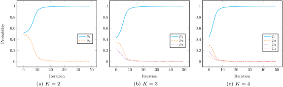
Figure 1: The probabilities of classes when applying entropy minimization on probabilities via gradient descent, where $K$ is the number of classes. The largest probability will get larger after each iteration of gradient descent.

Interpretation for Entropy-Based Methods

We take TENT (Wang et al. 2021) for example. To easily present our main find, we first consider the binary case, where the number of classes is 2, i.e., $K=2$. Let $c^{+}$ and $c^{-}$ denote the positive and negative labels. We denote $p(x;c^{+})$ and $p(x;c^{-})$ as the probabilities that the test sample $x$ belongs to the positive and negative labels.

A-step: In the entropy-based TTA, a test sample goes through the deep model and obtains a $P(x)=\sigma(f_{t}(x))=[p(x;c^{+}),p(x;c^{-})]$ in the forward process. This process is similar to the clustering methods that assign the cluster to each data point. Please note that clustering methods further assign the nearest center via $\hat{c}(x)=\mathop{\arg\max}\limits_{c\in\{c^{+},c^{-}\}}p(x;c)$. EBTTA does not explicitly perform this step and keeps uncertain probabilities.

U-step: With the probability $P(x)$ for each sample, EBTTA uses the entropy loss to update the model. This process is similar to the clustering methods that update the centers. In the clustering methods, the $i$-th center is updated by averaging features of the samples that were assigned to the $i$-th center in the A-step. We first give a lemma, which shows that the entropy loss also aims to further increase the samples’ probability belonging to the $i$-th class, where these samples have the largest probability of the $i$-th class in the forward process. The backward process of EBTTA is very similar to the U-step of clustering, that is both methods use the assigned samples to update the model/centers.

For the entropy loss, we have the following lemma, which indicates that the entropy loss aims to minimize the uncertainty of each sample that is assigned to the class labels.

Lemma 1

The entropy loss would increase the probability of the class with the largest value, and decrease the sum of probabilities of the other classes.

It is easy to verify in the binary classification. Without loss of generality, suppose that $p(x;c^{+})>p(x;c^{-})$ in the A-step. Since SGD is used to update the model, i.e., $p(x;c^{+})\leftarrow p(x;c^{+})-\alpha\frac{dH(x)}{dp(x;c^{+})}$ ($\alpha>0$ is the learning rate), we only need to show that the gradient of the maximum class is less than zero, i.e., $\frac{dH(x)}{dp(x;c^{+})}<0$.

Let $p=p(x;c^{+})$, the derivative of entropy $H(x)$ with respect to $p$ is calculated by:

$$\frac{dH(x)}{dp} =\frac{d[-p\mathrm{log}p-(1-p)\mathrm{log}(1-p)]}{dp}$$ (2)

$$=\mathrm{log}\frac{1-p}{p}.$$

According to the assumption $p(x;c^{+})>p(x;c^{-})$ and $p(x;c^{+})+p(x;c^{-})=1$, we have $p(x_{c^{+}};c^{+})>\frac{1}{2}$. Therefore we have $\frac{dH(x)}{dp(x;c^{+})}<0$ since $\mathrm{log}\frac{1-p}{p}<0$. The update of the entropy loss by gradient descent can make $p(x;c^{+})$ larger.

The proof of multi-classification is given in Appendix B. Lemma 1 shows that the entropy loss reduces the uncertainty by further increasing the largest probability. For example, if $p(x;c^{+})>p(x;c^{-})$, the entropy loss will further increase the value of $p(x;c^{+})$ and thus decrease the probability of $p(x;c^{-})$. Some examples of the changes of probabilities after each iteration via entropy minimization are shown in Figure 1.

Remark 1: Lemma 1 does not mean that the largest probabilities of the classes in the mini-batch are always the largest. It only always holds when the batch size is 1. The gradients of multiple samples will be averaged to update a shared model. Hence, the largest probability of the data point may be changed due to the averaged gradients. This is similar to the clustering method. For example, $x_{1}$ is assigned to the positive class in the current iteration. After the update of cluster centers, $x_{1}$ may possibly be assigned to the negative class in the next iteration.

From the view of clustering, we can gain a more thorough understanding of EBTTA. Several questions can be more easily answered.

Q1: What information does the source model provide during adaptation?

In the TTA method, the source model is used as an initiated model to be updated. From the clustering view, the source model also provides the initial probabilities belonging to the $K$ classes. As we had discussed above, the entropy loss tries to further increase the largest probability of each test sample. Thus the initial source model is very important, and we can achieve excellent performance with good initial probabilities, otherwise the entropy loss may hurt the performances. This is similar to clustering methods that are also sensitive to the initial cluster centers.

Q2: Why do some EBTTA works need to select low-entropy samples?

Several methods, e.g., ETA (Niu et al. 2022) and SAR (Niu et al. 2023), had proposed to use only the low-entropy samples to update the model, and the high-entropy samples were removed. The effectiveness of this technique has been verified by experiments but a detailed analysis is missing. From the clustering view, we can easily give an explanation: outliers should be suppressed. In Remark 1, we had shown that the gradients will be averaged to update the model. When the directions of the gradients are wrong (caused by the outliers), they may cause more mistakes in the updated model.

Q3: Why is batch size so important for EBTTA?

The EBTTA methods are sensitive to the batch size (Wang et al. 2021; Nguyen et al. 2023). This can also be easily answered using the clustering view. As the deep model is updated via the averaged assigned samples’ gradients, more samples can provide more stable gradients. That is, when the batch size is small, the variance will be large. This is similar to the clustering methods, where the centers are updated by averaging features of assigned samples. When the number of samples is small, the calculated centers also will have large variance.

def forward(x, counter):

outputs = model(x)

aug_outputs = model(aug(x)).detach()

# Robust Label Assignment

outputs = (outputs + aug_outputs)/2

ent = softmax_entropy(outputs)

# Weight Adjustment

weight = ent.pow(-$\tau$).detach()

loss = (weight * ent).mean()

loss = loss / Q

loss.backward()

# Gradient Accumulation

if counter % Q == 0:

optimizer.step()

optimizer.zero_grad()

return outputs

Algorithm 1 Pytorch-like pseudo-code for TTC; $x$ is a batch of unlabeled test samples; $counter$ is the number of batches encountered.

Method	gaus	shot	impul	defcs	gls	mtn	zm	snw	frst	fg	brt	cnt	els	px	jpg	Avg
SOURCE	27.7	34.3	27.1	53.0	45.7	65.2	58.0	74.9	58.7	74.0	90.7	53.3	73.4	41.5	69.7	56.5
NORM	71.9	73.8	63.9	87.4	65.0	86.2	87.9	82.7	82.5	84.9	91.9	86.7	76.8	80.6	72.9	79.7
T3A	32.6	38.6	28.9	55.4	48.3	66.5	60.7	74.9	59.6	74.2	90.4	53.9	73.2	42.9	69.4	58.0
ETA	71.8	73.6	63.9	87.2	65.1	86.3	87.7	82.4	82.1	84.8	91.5	87.0	76.2	80.0	72.2	79.5
TIPI	75.2	77.1	67.4	84.7	66.3	82.8	86.1	83.4	82.6	83.5	90.9	85.5	76.8	79.1	77.8	79.9
TENT	75.7	77.1	67.8	87.7	68.6	86.9	88.6	84.1	83.8	86.2	92.0	87.8	77.6	83.3	75.4	81.5
TTC(ours)	77.6	79.4	70.1	89.0	70.4	88.0	89.8	85.4	85.6	87.3	92.7	90.1	79.7	84.6	77.4	83.1

Table 1: Accuracy(%) of different methods on CIFAR-10-C with WideResnet28-10.

Method	gaus	shot	impul	defcs	gls	mtn	zm	snw	frst	fg	brt	cnt	els	px	jpg	Avg
SOURCE	16.6	15.0	3.0	8.5	9.9	7.4	8.4	8.5	5.9	1.4	10.8	1.2	9.7	11.7	13.6	8.8
NORM	55.1	54.5	48.5	54.2	50.4	52.7	55.5	52.7	54.0	32.4	57.7	35.7	52.2	54.7	55.2	51.0
T3A	19.5	18.2	5.3	9.7	11.3	9.3	10.5	10.4	7.6	1.9	13.1	1.2	11.7	13.5	15.3	10.6
ETA	50.2	48.1	44.0	49.7	45.8	49.3	50.8	49.1	49.5	43.0	53.1	37.4	48.6	49.1	50.2	47.9
TIPI	38.1	39.7	29.1	43.1	34.2	36.3	38.9	41.6	39.0	13.5	48.6	6.4	38.4	40.9	37.8	35.0
TENT	52.2	51.8	49.3	50.2	46.2	51.7	52.5	51.7	51.7	45.3	53.7	24.9	47.9	52.8	50.2	48.8
TTC(ours)	54.1	53.9	50.9	53.7	49.3	52.8	54.9	53.5	53.7	46.7	55.9	40.4	50.3	53.7	52.7	51.8

Table 2: Accuracy(%) of different methods on on CIFAR-100-C with WideResnet28-10.

Method	gaus	shot	impul	defcs	gls	mtn	zm	snw	frst	fg	brt	cnt	els	px	jpg	Avg
SOURCE	2.2	2.9	1.9	17.9	9.8	14.8	22.5	16.9	23.3	24.4	58.9	5.4	17.0	20.6	31.6	18.0
NORM	15.6	16.4	16.3	15.4	15.8	27.1	39.8	35.0	33.8	48.7	65.9	17.3	45.2	50.2	40.7	32.2
T3A	2.2	2.8	1.9	12.8	7.5	9.7	16.6	13.2	17.4	20.4	45.5	4.5	15.4	15.5	23.0	13.9
ETA	29.2	31.8	31.0	20.3	21.4	44.9	50.3	50.2	43.5	59.2	66.7	34.3	56.9	59.8	53.9	43.6
TIPI	21.6	5.9	27.3	4.9	4.2	20.3	36.8	41.9	38.5	46.7	63.1	3.0	50.3	54.1	52.2	31.4
TENT	25.9	30.8	30.3	25.0	25.1	45.4	51.0	50.1	37.4	59.2	67.7	14.7	57.1	60.3	54.4	42.3
TTC(ours)	31.5	32.9	33.0	30.0	29.1	43.0	51.4	49.3	43.6	59.4	68.7	32.1	56.2	60.4	54.3	45.0

Table 3: Accuracy(%) of different methods on ImageNet-C with Resnet50.

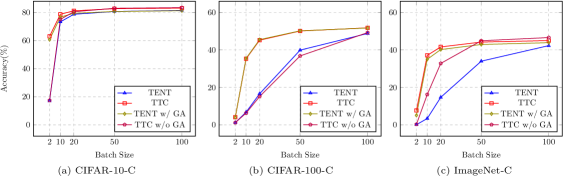
Figure 2: Accuracy(%) on various datasets with different batch sizes. Gradient accumulation (GA) can boost performance significantly when the batch size is small.

Test-Time Clustering (TTC)

Based on the observations that EBTTA is sensitive to initial probabilities, outliers, and batch size, we propose to improve TENT from these three aspects accordingly. First, we suggest to obtain a more robust initial label assignment in order to get high-quality initial probabilities. Second, we propose to adjust the weight of test samples to alleviate the negative effects of outliers. Third, we recommend to use gradient accumulation to overcome the problem of small batch size.

Robust Label Assignment

As discussed in Q1, we can see that label assignment in the A-step is very important for the EBTTA, which also provides a good initial probability for each test sample.

In order to get a better assignment, we simply apply data augmentation inspired by the success of self-supervised learning. Then we combine the two predictions to obtain a more robust probability:

$$\bar{f}_{t}(x)\leftarrow\frac{f_{t}(x)+f_{t}(\mathrm{aug}(x))}{2},\bar{P}(x)=\sigma(\bar{f}_{t}(x)),$$ (3)

where $\mathrm{aug}(x)$ is the data augmentation function, and $\bar{P}(x)$ is a more robust initial probability for test sample $x$. Here we only choose horizontal flip which is a weak augmentation function, rather than other strong augmentation functions. This is because a weakly-augmented unlabeled sample can preserve more semantic information and generate a better pseudo-label than the strongly augmented functions (Yang et al. 2022). Note that stop-gradient operation is applied to $f_{t}(\mathrm{aug}(x))$ in Eq. (3), which can save computational resources.

Weight Adjustment

With the robust label assignment, the entropy becomes

$$\bar{H}(x_{i})=-\sum_{k=1}^{K}[\sigma(\bar{f}_{t}(x_{i})]_{k}\mathrm{log}[\sigma(\bar{f}_{t}(x_{i})]_{k}.$$ (4)

We can see that each sample has the same weight $1/N$ in Eq. (1). According to the discussion in Q2, we set high weights for low-entropy samples and low weights for high-entropy samples, which is inspired by sample-weighted clustering (Yu, Yang, and Lee 2011) where different samples may have different weights and outliers have lower weights. The weight is formulated as

$$w_{i}=\frac{[\bar{H}(x_{i})]^{-\tau}}{N},$$ (5)

where $\tau>0$ is a hyper-parameter. The loss function is calculated as:

$$\mathcal{L}_{\mathrm{TTC}}=\sum_{i=1}^{N}w_{i}\bar{H}(x_{i}).$$ (6)

Note that stop-gradient operation is applied to $w_{i}$ in Eq.(5), which is treated as a constant term.

Gradient Accumulation

When the batch size is limited, we propose to use gradient accumulation to collect information from multiple batches, which is equivalent to increasing the batch size (Lin et al. 2017). In practice, we don’t update the parameters immediately once we get the gradient of one batch. Instead, we collect the gradients for $Q$ batches and then conduct gradient descending.

The pseudo-code of our method is shown in Algorithm 1.

Experiments

In this section, we evaluate our method on various datasets. Besides, we have conducted ablation study to explore the characteristics of our methods. Further, we visualize the feature distribution of different methods.

Datasets and Evaluation Metric

Datasets

We conduct experiments on three common benchmark datasets for TTA evaluation:

• CIFAR-10/100-C (Hendrycks and Dietterich 2019): The source models are trained on the training set of CIFAR-10/100 (Krizhevsky, Hinton et al. 2009), which contains 50,000 images with 10/100 classes. Then models are tested on CIFAR-10/100-C, which contains 10,000 images. CIFAR-10/100-C is the corrupted version of the test set of CIFAR-10/100.

• ImageNet-C (Hendrycks and Dietterich 2019): The source models are first trained on the training set of ImageNet (Russakovsky et al. 2015), which includes 1.2 million images with 1,000 classes. Models are then adapted on the corrupted test set ImageNet-C including 50,000 images.

Corruption types include Gaussian noise (gaus), shot noise (shot), impulse noise (impul), defocus blur (defcs), glass blur (gls), motion blur (mtn), zoom blur (zm), snow (snw), frost (frst), fog (fg), brightness (brt), contrast (cnt), elastic transform (els), pixelate (px), and JPEG compression (jpg). For all datasets, we choose the highest corruption severity level for testing.

Evaluation Metric

We use accuracy to measure the performance of methods on datasets. Here we denote the number of test samples as $N_{\mathrm{test}}$. Accuracy is a widely used measurement in classification tasks, which can be calculated as:

$$\mathrm{Accuracy}=\frac{\sum_{i=1}^{N_{\mathrm{test}}}\mathbb{I}_{\{\mathop{\arg\max}P(x_{i})==y_{i}\}}}{N_{\mathrm{test}}},$$ (7)

where $y_{i}$ is the true label of $x_{i}$.

Compared Methods

We compare our method with the following TTA methods:

• SOURCE: the baseline method where no adaptation is conducted.

• NORM (Schneider et al. 2020)(NIPS 2020): this method only updates the statistics of BN layers.

• T3A (Iwasawa and Matsuo 2021)(NIPS 2021): it constructs and updates pseudo-prototype for each class and performs nearest neighbour classification during adaptation.

• TENT (Wang et al. 2021)(ICLR 2021): it updates the BN layers by entropy minimizing via SGD.

• ETA (Niu et al. 2022)(ICML 2022): it conducts selective entropy minimizing during adaptation.

• TIPI (Nguyen et al. 2023)(CVPR 2023): this method uses a variance regularizer to adapt the model.

Method	gaus	shot	impul	defcs	gls	mtn	zm	snw	frst	fg	brt	cnt	els	px	jpg	Avg
SOURCE	79.8	81.0	69.2	81.0	80.5	79.4	82.2	81.2	79.6	39.2	85.2	21.1	83.3	85.8	87.4	74.4
NORM	88.2	88.5	85.9	87.7	84.6	86.5	88.0	85.6	87.0	70.8	88.8	80.5	85.6	88.1	88.6	85.6
T3A	79.9	80.8	69.3	80.4	80.5	78.4	82.0	79.3	78.6	36.3	84.2	20.9	82.6	84.5	86.6	73.6
ETA	87.8	88.0	85.7	87.0	84.2	86.0	87.8	85.4	86.5	71.3	88.4	80.3	85.2	87.7	87.9	85.3
TIPI	87.0	86.7	84.9	84.9	82.7	84.3	87.2	86.0	86.3	70.9	88.6	66.8	84.5	86.7	87.7	83.7
TENT	88.8	89.6	86.7	88.5	85.4	87.2	89.4	87.7	89.0	82.6	90.2	83.6	86.8	89.2	88.8	87.6
TTC(ours)	89.6	89.8	87.6	89.4	86.0	88.2	90.4	88.1	88.9	83.2	90.7	84.5	87.6	89.9	89.8	88.2

Table 4: Accuracy(%) of different methods on CIFAR-10-C with Resnet18.

Method	gaus	shot	impul	defcs	gls	mtn	zm	snw	frst	fg	brt	cnt	els	px	jpg	Avg
SOURCE	70.3	72.5	63.0	83.8	80.3	81.0	85.9	83.3	80.2	42.1	88.7	18.9	84.3	87.1	88.8	74.0
NORM	78.8	78.5	76.5	78.2	73.6	76.6	79.4	75.0	76.0	62.9	81.9	70.4	76.5	78.9	79.8	76.2
T3A	71.3	73.2	64.1	83.3	80.0	80.5	85.3	83.1	80.1	41.0	88.1	19.2	83.7	86.7	88.0	73.8
ETA	78.6	79.6	76.4	79.0	74.7	77.6	79.5	75.1	77.0	64.6	81.0	70.2	76.1	78.4	79.6	76.5
TIPI	73.9	77.7	69.3	67.2	70.2	69.6	72.2	71.4	77.7	50.6	80.6	46.6	71.2	75.8	80.1	70.3
TENT	77.4	78.2	75.9	75.6	70.8	71.3	80.4	76.5	76.2	72.8	79.9	63.5	72.2	76.9	77.8	75.0
TTC(ours)	81.9	80.8	79.5	80.0	74.6	76.1	83.4	80.8	80.7	76.7	82.6	74.9	75.9	79.8	80.8	79.2

Table 5: Accuracy(%) of different methods on CIFAR-10-C with Resnet50.

Implementation Details

For a fair comparison, all methods use the same model and the same optimizer. Following TIPI (Nguyen et al. 2023), for CIFAR-10-C and CIFAR-100-C, we use model WideResnet28-10 (Zagoruyko and Komodakis 2016) and optimizer Adam (Kingma and Ba 2014) as a default setting; for ImageNet-C, we use model Resnet50 (He et al. 2016) and optimizer SGD as default. All methods share the same learning rate 0.001 for CIFAR-10/100-C and 0.002 for ImageNet-C. The batch size $N$ is 100 for all methods. For TTC, we set $\tau=0.5$ and $Q=\frac{200}{N}$ and only update BN layers as TENT does. Other details of our method can be found in the provided code.

Comparison on Various Datasets

The comparison results are shown in Table 1, Table 2 and Table 3. The results show that our method can achieve consistent improvements w.r.t. accuracy on all three datasets. The average (avg) accuracy is calculated on all corruption types. More detailed analysis is as follows.

CIFAR-10-C. The results are shown in Table 1. We can see that our method achieves the best average accuracy 83.1%, which is 1.6% superior to the second-best method TENT. Besides, TTC performs better TENT on all corruption types. Specifically, TTC is 2.3% superior to TENT w.r.t. shot corruption. Since TENT is the most relevant work, the comparison results indicate that the proposed improvements are effective.

CIFAR-100-C. As shown in Table 2, our model still achieves the best average accuracy, which is 0.8% better than the second-best model NORM. Although NORM performs better than our method in most corruption types, our method achieves more stable performances. For example, NORM is only 0.3% better than TTA w.r.t. frst corruption while our method is 14.3% better than NORM w.r.t. fg corruption.

ImageNet-C. The results of Table 3 show that our method achieves the best average accuracy 45.0%, and the accuracy of the second-best model ETA is 43.6%. Note that previous entropy-based methods achieve excellent performance, even so, our method performs better than them.

Ablation Studies

In this set of experiments, we conduct ablation studies to analyze the characteristics of our method.

Analysis of Different Components

We conduct experiments to analyze the improvements caused by different components of our method individually. Specifically, we use TENT as the base model. We apply different components individually to TENT and the average accuracies for datasets are shown in Table 6. We shall see Robust Label Assignment (RLA) and weight adjustment (WA) can both bring about improvements for TENT on CIFAR-10-C and ImageNet-C. Gradient accumulation (GA) can make significant improvements on CIFAR-100-C and ImageNet-C. Please note that the batch size in Table 6 is 100, which is not too small. Thus it may be the reason why TENT+GA has similar result to TENT on CIFAR-10-C dataset. Detailed analysis of GA for different batch sizes can be found in Section Analysis of Different Batch Sizes, where GA can boost the performance significantly when the batch size is small.

Method	CIFAR-10-C	CIFAR-100-C	ImageNet-C
TENT	81.5	48.8	42.3
+RLA	82.6(+1.1)	49.2(+0.4)	45.7(+3.4)
+WA	82.3(+0.8)	48.7(-0.1)	44.5(+2.2)
+GA	81.2(-0.3)	51.7(+2.9)	43.9(+1.6)

Table 6: Effects of different components applied to TENT individually.

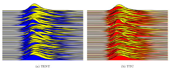
Figure 3: Density plots of test-time feature distribution on ImageNet-C with Gaussian noise. The color for the feature distribution of the supervised learning as reference is yellow. The color for the feature distribution of TENT is blue. The color for the feature distribution of TTC is red. Each horizontal axis represents a channel. More overlapping areas means more alignment, hence TTC is more aligned with supervised learning.

Analysis of Different Augmentations

We conduct experiments to explore the effect of different augmentation functions $\mathrm{aug}(x)$ in Eq.(3). The augmentation functions are horizontal flip (HorFlip), vertical flip (VerFlip), random rotation (RandRot), random resized crop (RRCrop), and Gaussian noise (GausNoise). From the average accuracies for datasets in Table 7, we shall see that horizontal flip provides a better pseudo-label and makes the performance better.

Aug	CIFAR-10-C	CIFAR-100-C	ImageNet-C
HorFlip	83.1	51.8	45.0
VerFlip	74.0	36.2	37.2
RandRot	74.8	30.2	35.5
RRCrop	77.1	40.0	38.3
GausNoise	82.0	48.9	43.6

Table 7: Ablation study of our method varying augmentation function.

Analysis of Different $\tau$

In this part, we explore the sensitivity to hyper-parameter $\tau$ in Eq.(5) of our method. When $\tau=\infty$, only the entropy loss of the sample with the highest weight will be considered in a batch during adaptation. When $\tau=0$, each sample shares the same weight in the batch. As shown in Table 8, the choosing of $\tau$ has a great impact on the performance. Our method strikes a good balance w.r.t. average accuracies on all datasets when $\tau$ is a moderate value 0.5.

$\tau$	CIFAR-10-C	CIFAR-100-C	ImageNet-C
10	10.7	47.0	0.2
5	80.6	41.9	0.3
1	83.9	48.5	44.9
0.5	83.1	51.8	45.0
0.1	82.6	52.0	45.2
0.05	82.5	52.0	45.3

Table 8: Ablation study of our method with different $\tau$.

Analysis of Different Batch Sizes

We further conduct an ablation study to explore the effect of the batch size, and the average accuracies on datasets are shown in Figure 2. We shall see that all four methods perform better when batch size increases. Moreover, when applying gradient accumulation (GA) for small batch sizes, we can get a large performance improvement for TENT and TTC.

Analysis of Different Models

We also test our method on CIFAR-10-C using other models: ResNet18 (He et al. 2016) and ResNet50 (He et al. 2016). The results are shown in Table 4 and Table 5, which demonstrates that our methods can keep leading performance with various models compared to other methods.

Feature Visualization

We follow  (Wang et al. 2021; Nguyen et al. 2023; Mirza et al. 2022) to draw the density plots of the feature distributions. Figure 3 compares the feature distributions obtained by TENT and TTC on ImageNet-C with Gaussian noise. The feature distribution for supervised learning serves as a reference target. We can see that the feature distribution of our method can be more aligned with that of supervised learning, which implies a better performance.

Conclusion

In this paper, we revisited existing EBTTA methods from the view of clustering. We found that the forward process can be interpreted as the label assignment while the backward process of EBTTA can be interpreted as the update of centers in clustering. This view can guide us to improve EBTTA by overcoming weaknesses in clustering methods, which are sensitive to initial assignments, outliers, and batch size. We proposed to assign robust labels, adjust weights, and accumulate gradients. Conducted experimental results have demonstrated the superiority of our proposed method. In our future work, we wish to give a better theoretical explanation for more test-time adaptation methods.

Appendix A Mini-Batch K-Means

Inspired by DeepCluster (Caron et al. 2018), we can theoretically express the learning procedure as:

$$\min\limits_{C}\frac{1}{N}\sum_{i=1}^{N}\min\limits_{y_{i}}\left(\parallel z(x_{i})-Cy_{i}\parallel_{2}^{2}\right)$$ (8)

where $z(x_{i})$ is the feature of sample $x_{i}$, $y_{i}$ is the assignment result of $x_{i}$, and $C$ is the matrix of centers. The problem in Eq. (8) can be solved by an alternating algorithm, fixing one set of variables while solving for the other set. Formally, we can alternate between solving these two sub-problems:

$$y_{i}^{j}\leftarrow\arg\min\limits_{y_{i}}\parallel z(x_{i})-C^{j-1}y_{i}\parallel_{2}^{2},$$ (9)

$$C^{j}\leftarrow\arg\min\limits_{C}\frac{1}{N}\sum_{i=1}^{N}\left(\parallel z(x_{i})-Cy_{i}^{j}\parallel_{2}^{2}\right),$$ (10)

where $j$ is the time step of alternation. We can see that Eq. (9) is the A-step while Eq. (10) is the U-step.

Appendix B The Proof of Multi-classification in the Lemma 1

We assume that in probabilities $P=\{p_{i}\}_{i=1}^{K}$ (we omit the symbol $x$ for simplicity), the change of the largest one $p_{m}$ is the opposite of all the other possibilities, for example, when $p_{m}$ increases, $\{p_{i}\}_{i\neq m}$ decrease (a natural result of the softmax function):

$$p_{1}\leftarrow p_{1}+dp_{1}$$ (11)

$$\vdots$$

$$p_{m}\leftarrow p_{m}+dp_{m}$$

$$\vdots$$

$$p_{K}\leftarrow p_{K}+dp_{K},$$

where $dp_{m}>0$, $dp_{i}<0$($i\neq m$).

Since the probabilities sum up to 1, we have:

$$p_{m}+\sum_{i\neq m}p_{i}=1,$$ (12)

and

$$p_{m}+dp_{m}+\sum_{i\neq m}(p_{i}+dp_{i})=1.$$ (13)

Therefore,

$$-\sum_{i\neq m}\frac{dp_{i}}{dp_{m}}=-\frac{d\sum_{i\neq m}p_{i}}{dp_{m}}=-\frac{d(1-p_{m})}{p_{m}}=1.$$ (14)

The total derivative of $H$ w.r.t. $p_{m}$ is:

$$\frac{dH}{dp_{m}}(P)= \sum_{i=1}^{K}\frac{\partial H}{\partial p_{i}}(P)\cdot\frac{dp_{i}}{dp_{m}}$$ (15)

$$= \frac{\partial H}{\partial p_{m}}(P)+\sum_{i\neq m}\frac{\partial H}{\partial p_{i}}(P)\cdot\frac{dp_{i}}{dp_{m}}$$

$$= -(1+\mathrm{log}(p_{m}))+\sum_{i\neq m}\frac{dp_{i}}{dp_{m}}[-(1+\mathrm{log}(p_{i})]$$

$$= -(1+\mathrm{log}(p_{m}))-\sum_{i\neq m}\frac{dp_{i}}{dp_{m}}$$

$$-\sum_{i\neq m}\frac{dp_{i}}{dp_{m}}\mathrm{log}(p_{i}).$$

Substituting Eq. (14) into Eq. (LABEL:eq2) we have:

$$\frac{dH}{dp_{m}}(P)=-\mathrm{log}(p_{m})-\sum_{i\neq m}\frac{dp_{i}}{dp_{m}}\mathrm{log}(p_{i}).$$ (17)

Suppose that the second largest probability $p_{n}=\mathrm{max}(\{p_{i}\}_{i\neq m})$, then considering $\frac{dp_{i}}{dp_{m}}<0(i\neq m)$ and Eq. (14) we have:

$$-\sum_{i\neq m}\frac{dp_{i}}{dp_{m}}\mathrm{log}(p_{i})\leq-\sum_{i\neq m}\frac{dp_{i}}{dp_{m}}\mathrm{log}(p_{n})=\mathrm{log}(p_{n}).$$ (18)

Since the largest probability $p_{m}$ must hold $p_{m}>p_{n}$, substituting Eq. (18) into Eq. (17) we have :

$$\frac{dH}{dp_{m}}(P)\leq-\mathrm{log}(p_{m})+\mathrm{log}(p_{n})<0.$$ (19)

Therefore, the minimizing of entropy loss via gradient descent can increase the largest probability.

References

- Béjar Alonso (2013) Béjar Alonso, J. 2013. K-means vs Mini Batch K-means: a comparison.
- Bjorck et al. (2018) Bjorck, N.; Gomes, C. P.; Selman, B.; and Weinberger, K. Q. 2018. Understanding batch normalization. Advances in neural information processing systems, 31.
- Bottou and Bengio (1994) Bottou, L.; and Bengio, Y. 1994. Convergence properties of the k-means algorithms. Advances in neural information processing systems, 7.
- Caron et al. (2018) Caron, M.; Bojanowski, P.; Joulin, A.; and Douze, M. 2018. Deep clustering for unsupervised learning of visual features. In Proceedings of the European conference on computer vision (ECCV), 132–149.
- Celebi, Kingravi, and Vela (2013) Celebi, M. E.; Kingravi, H. A.; and Vela, P. A. 2013. A comparative study of efficient initialization methods for the k-means clustering algorithm. Expert systems with applications, 40(1): 200–210.
- Chavan et al. (2015) Chavan, M.; Patil, A.; Dalvi, L.; and Patil, A. 2015. Mini batch K-Means clustering on large dataset. Int. J. Sci. Eng. Technol. Res, 4(07): 1356–1358.
- Döbler, Marsden, and Yang (2023) Döbler, M.; Marsden, R. A.; and Yang, B. 2023. Robust mean teacher for continual and gradual test-time adaptation. In Proceedings of the IEEE/CVF Conference on Computer Vision and Pattern Recognition, 7704–7714.
- Dosovitskiy et al. (2020) Dosovitskiy, A.; Beyer, L.; Kolesnikov, A.; Weissenborn, D.; Zhai, X.; Unterthiner, T.; Dehghani, M.; Minderer, M.; Heigold, G.; Gelly, S.; et al. 2020. An image is worth 16x16 words: Transformers for image recognition at scale. arXiv preprint arXiv:2010.11929.
- Guo et al. (2017) Guo, X.; Liu, X.; Zhu, E.; and Yin, J. 2017. Deep clustering with convolutional autoencoders. In Neural Information Processing: 24th International Conference, ICONIP 2017, Guangzhou, China, November 14-18, 2017, Proceedings, Part II 24, 373–382. Springer.
- He et al. (2016) He, K.; Zhang, X.; Ren, S.; and Sun, J. 2016. Deep residual learning for image recognition. In Proceedings of the IEEE conference on computer vision and pattern recognition, 770–778.
- Hendrycks and Dietterich (2019) Hendrycks, D.; and Dietterich, T. 2019. Benchmarking neural network robustness to common corruptions and perturbations. arXiv preprint arXiv:1903.12261.
- Iwasawa and Matsuo (2021) Iwasawa, Y.; and Matsuo, Y. 2021. Test-time classifier adjustment module for model-agnostic domain generalization. Advances in Neural Information Processing Systems, 34: 2427–2440.
- Kingma and Ba (2014) Kingma, D. P.; and Ba, J. 2014. Adam: A method for stochastic optimization. arXiv preprint arXiv:1412.6980.
- Kirillov et al. (2023) Kirillov, A.; Mintun, E.; Ravi, N.; Mao, H.; Rolland, C.; Gustafson, L.; Xiao, T.; Whitehead, S.; Berg, A. C.; Lo, W.-Y.; et al. 2023. Segment anything. arXiv preprint arXiv:2304.02643.
- Krizhevsky, Hinton et al. (2009) Krizhevsky, A.; Hinton, G.; et al. 2009. Learning multiple layers of features from tiny images.
- Liang, Hu, and Feng (2020) Liang, J.; Hu, D.; and Feng, J. 2020. Do we really need to access the source data? source hypothesis transfer for unsupervised domain adaptation. In International conference on machine learning, 6028–6039. PMLR.
- Lin et al. (2017) Lin, Y.; Han, S.; Mao, H.; Wang, Y.; and Dally, W. J. 2017. Deep gradient compression: Reducing the communication bandwidth for distributed training. arXiv preprint arXiv:1712.01887.
- Mirza et al. (2022) Mirza, M. J.; Micorek, J.; Possegger, H.; and Bischof, H. 2022. The norm must go on: Dynamic unsupervised domain adaptation by normalization. In Proceedings of the IEEE/CVF Conference on Computer Vision and Pattern Recognition, 14765–14775.
- Nguyen et al. (2023) Nguyen, A. T.; Nguyen-Tang, T.; Lim, S.-N.; and Torr, P. H. 2023. TIPI: Test Time Adaptation with Transformation Invariance. In Proceedings of the IEEE/CVF Conference on Computer Vision and Pattern Recognition, 24162–24171.
- Niu et al. (2022) Niu, S.; Wu, J.; Zhang, Y.; Chen, Y.; Zheng, S.; Zhao, P.; and Tan, M. 2022. Efficient test-time model adaptation without forgetting. In International conference on machine learning, 16888–16905. PMLR.
- Niu et al. (2023) Niu, S.; Wu, J.; Zhang, Y.; Wen, Z.; Chen, Y.; Zhao, P.; and Tan, M. 2023. Towards stable test-time adaptation in dynamic wild world. arXiv preprint arXiv:2302.12400.
- Redmon et al. (2016) Redmon, J.; Divvala, S.; Girshick, R.; and Farhadi, A. 2016. You only look once: Unified, real-time object detection. In Proceedings of the IEEE conference on computer vision and pattern recognition, 779–788.
- Ren et al. (2015) Ren, S.; He, K.; Girshick, R.; and Sun, J. 2015. Faster r-cnn: Towards real-time object detection with region proposal networks. Advances in neural information processing systems, 28.
- Russakovsky et al. (2015) Russakovsky, O.; Deng, J.; Su, H.; Krause, J.; Satheesh, S.; Ma, S.; Huang, Z.; Karpathy, A.; Khosla, A.; Bernstein, M.; et al. 2015. Imagenet large scale visual recognition challenge. International journal of computer vision, 115: 211–252.
- Schneider et al. (2020) Schneider, S.; Rusak, E.; Eck, L.; Bringmann, O.; Brendel, W.; and Bethge, M. 2020. Improving robustness against common corruptions by covariate shift adaptation. Advances in neural information processing systems, 33: 11539–11551.
- Tomar et al. (2023) Tomar, D.; Vray, G.; Bozorgtabar, B.; and Thiran, J.-P. 2023. TeSLA: Test-Time Self-Learning With Automatic Adversarial Augmentation. In Proceedings of the IEEE/CVF Conference on Computer Vision and Pattern Recognition, 20341–20350.
- Wang et al. (2021) Wang, D.; Shelhamer, E.; Liu, S.; Olshausen, B.; and Darrell, T. 2021. Tent: Fully Test-Time Adaptation by Entropy Minimization. In International Conference on Learning Representations.
- Wang et al. (2022) Wang, Q.; Fink, O.; Van Gool, L.; and Dai, D. 2022. Continual test-time domain adaptation. In Proceedings of the IEEE/CVF Conference on Computer Vision and Pattern Recognition, 7201–7211.
- Wang et al. (2023) Wang, S.; Zhang, D.; Yan, Z.; Zhang, J.; and Li, R. 2023. Feature alignment and uniformity for test time adaptation. In Proceedings of the IEEE/CVF Conference on Computer Vision and Pattern Recognition, 20050–20060.
- Yang et al. (2022) Yang, X.; Hu, X.; Zhou, S.; Liu, X.; and Zhu, E. 2022. Interpolation-based contrastive learning for few-label semi-supervised learning. IEEE Transactions on Neural Networks and Learning Systems.
- Yu, Yang, and Lee (2011) Yu, J.; Yang, M.-S.; and Lee, E. S. 2011. Sample-weighted clustering methods. Computers & mathematics with applications, 62(5): 2200–2208.
- Yuan, Xie, and Li (2023) Yuan, L.; Xie, B.; and Li, S. 2023. Robust test-time adaptation in dynamic scenarios. In Proceedings of the IEEE/CVF Conference on Computer Vision and Pattern Recognition, 15922–15932.
- Zagoruyko and Komodakis (2016) Zagoruyko, S.; and Komodakis, N. 2016. Wide residual networks. arXiv preprint arXiv:1605.07146.
- Zhang, Levine, and Finn (2022) Zhang, M.; Levine, S.; and Finn, C. 2022. Memo: Test time robustness via adaptation and augmentation. Advances in Neural Information Processing Systems, 35: 38629–38642.
- Zhao et al. (2023) Zhao, H.; Liu, Y.; Alahi, A.; and Lin, T. 2023. On Pitfalls of Test-Time Adaptation. In International Conference on Machine Learning, volume 202, 42058–42080.