Abstract

Experiencing domain shifts during test-time is nearly inevitable in practice and likely results in a severe performance degradation. To overcome this issue, test-time adaptation continues to update the initial source model during deployment. A promising direction are methods based on self-training which have been shown to be well suited for gradual domain adaptation, since reliable pseudo-labels can be provided. In this work, we address two problems that exist when applying self-training in the setting of test-time adaptation. First, adapting a model to long test sequences that contain multiple domains can lead to error accumulation. Second, naturally, not all shifts are gradual in practice. To tackle these challenges, we introduce GTTA. By creating artificial intermediate domains that divide the current domain shift into a more gradual one, effective self-training through high quality pseudo-labels can be performed. To create the intermediate domains, we propose two independent variations: mixup and light-weight style transfer. We demonstrate the effectiveness of our approach on the continual and gradual corruption benchmarks, as well as ImageNet-R. To further investigate gradual shifts in the context of urban scene segmentation, we publish a new benchmark: CarlaTTA. It enables the exploration of several non-stationary domain shifts.

1 Introduction

Figure 1: Illustration of a gradually evolving domain. In the beginning $t=0$, perfect classification is possible. At time step $t=1$, the domain has gradually changed and the original source decision boundary $\beta_{0}$ still separates both classes. When the domain further evolves ($t=2$), the original decision boundary cannot separate the data anymore. When updating the model through self-training at time step $t=1$, a good classification would still be possible at time step $t=2$, as indicated by the dashed line.

Deep neural networks achieve remarkable performance under the assumption that training and test data originate from the same distribution. However, when a neural network is deployed in the real world, this assumption is often violated. This effect is known as data shift Quiñonero-Candela . (2008) and leads to a potentially large drop in performance on the test data. While it is possible to improve robustness and generalization directly during training Hendrycks . (2019, 2021); Muandet . (2013); Tobin . (2017); Tremblay . (2018), the effectiveness remains limited due to the wide range of potential data shifts Mintun . (2021) that are unknown during training. Thus, another area of research, namely test-time adaptation (TTA), follows the idea to adapt the pre-trained source model during deployment, as the encountered test data provides information about the current distribution shift.

Recent work on TTA focuses on the setting where the model only has to adapt to a single test domain. Needless to say, in practice this setting is very unlikely; it is much more likely that a model encounters different domains without the knowledge when a change occurs. Q. Wang ., 2022 denotes the setting where a model is adapted during deployment to a sequence of test domains as continual test-time adaptation. Due to potentially infinitely long test sequences and the encounter of different domain shifts, test-time adaptation, which is usually based on self-training and entropy minimization, is prone to error accumulation Q. Wang . (2022).

Clearly, the larger a shift is, the more likely it becomes that a model introduces errors. In the case of self-training, this likely results in an unsuccessful model adaptation due to the lack of reliable pseudo-labels Kumar . (2020). On the contrary, Kumar ., 2020 showed both theoretically and empirically that a model can be adapted successfully if the experienced shifts are small enough. Hence, adaptation to large shifts can be successful if divided into smaller gradual shifts, as illustrated in Figure 1.

Looking at the nature of shifts in reality, for many applications they do not occur abruptly, but evolve gradually over time. While the change from day to night is only one example, Kumar ., 2020 mentions, among others, evolving road conditions Bobu . (2018) and sensor aging Vergara . (2012). Of course, gradual shifts are not given in all settings or the gap of the experienced gradual shift is still too large for a successful model adaptation. Therefore, we propose to leverage source data to artificially create intermediate domains where, optimally, correct labels can be utilized to prevent the incorporation of additional errors. Even though requiring source data can be a limitation, we argue that having access to the initial source data is commonly the case. Now, for the creation of the intermediate domains we suggest two independent approaches: the first is based on mixup where the intermediate domains are created by linearly interpolating source and test images. The second idea uses a content-preserving light-weight style transfer model that is adapted online to new target styles. Since mixup and style transfer have their limitations and only mitigate the current domain gap, we rely on self-training to close the remaining gap. Assuming that mixup or style transfer moves the model closer to the test distribution, better self-training through more reliable pseudo-labels can be performed.

To demonstrate the effectiveness of our approach, we consider the continual and gradual corruption benchmark, as well as ImageNet-R. Due to the lack of datasets containing non-stationary domain shifts, we introduce and publish a new benchmark for the task of urban scene segmentation: CarlaTTA. It includes various non-stationary domain shifts in the setting of autonomous driving. We achieve new state-of-the-art results on all benchmarks. We summarize our main contributions as follows:

• We introduce a new framework Gradual Test-time Adaptation (GTTA), which conducts effective self-training by converting the current arbitrary domain shift into a gradual one. This is achieved by generating artificial intermediate domains using either mixup or light-weight style transfer.

• We publish a new benchmark for urban scene segmentation that enables the exploration of several non-stationary domain shifts during test-time in the field of autonomous driving.

2 Related Work

Unsupervised Domain Adaptation Recently, there has been a growing interest in mitigating the distributional discrepancy between two domains using unsupervised domain adaptation (UDA). Common approaches for UDA try to align either the input space Hoffman . (2018); Marsden, Wiewel . (2022); Z. Wu . (2019), the feature space Q. Zhang . (2019); Marsden, Bartler . (2022), the output space Tsai . (2018, 2019), or several spaces in parallel Y. Li . (2019); Yang  Soatto (2020). One line of work relies on adversarial learning, where a domain classifier tries to discriminate whether some feature maps Ganin  Lempitsky (2015) or network outputs Tsai . (2018); Vu . (2019) belong to the source or target domain. It is also possible to exploit adversarial learning or adaptive instance normalization (AdaIN) Huang  Belongie (2017) for transferring the target style to source images Hoffman . (2018); Marsden, Wiewel . (2022). Lately, self-training has gained a lot of attraction Tranheden . (2021); Mei . (2020); P. Zhang . (2021); Hoyer . (2022); G. Li . (2020). Self-training utilizes a pre-trained (source) model to create predictions for the unlabeled target data. These predictions can then be treated as pseudo-labels to minimize, for example, the cross-entropy. Since high quality pseudo-labels are essential to this approach, most methods differ in how they select or create reliable pseudo-labels.

One-shot Unsupervised Domain Adaptation As pointed out in Luo ., 2020, even collecting unlabeled target data can be challenging. Therefore, Luo ., 2020 introduced one-shot UDA, where only one single target image is available during the model adaptation. To address this problem, Luo ., 2020 extends the adaptive instance normalization framework of Huang  Belongie, 2017 with a variational autoencoder. By selecting styles for which the segmentation model is uncertain, the domain gap is mitigated. Differently, X. Wu ., 2021 uses a style mixing component within the segmentation model and further adds patch-wise prototypical matching.

Test-time Adaptation Although generalizing to any test distribution would solve many problems, the lack of information about the test environment during training imposes a great challenge. However, during model deployment, one can gain some insight into the test distribution by using the current test sample(s). This circumstance is also exploited in recent work, where Schneider ., 2020 showed that even adapting the batch normalization (BN) statistics during test-time can significantly improve the performance on corrupted data. More sophisticated approaches perform source model optimization during test-time. For example, D. Wang ., 2020 update the BN layers by entropy minimization. M. Zhang ., 2021 create an ensemble prediction through test-time augmentation Krizhevsky . (2009) and then minimize the entropy with respect to all parameters. Other methods rely on self-supervised learning, using either pre-text tasks to adapt the model Y. Sun . (2020); Liu . (2021); Bartler . (2022) or apply contrastive learning D. Chen . (2022). Recent works make use of diversity regularizers Liang . (2020); Mummadi . (2021) to prevent the collapse to trivial solutions potentially caused by confidence maximization.

Continual Test-time Adaptation Continual test-time adaptation considers online TTA with continually changing target domains. While some of the existing methods can be applied to the continual setting, such as the online version of TENT D. Wang . (2020), they are often prone to error accumulation due to miscalibrated predictions Q. Wang . (2022). CoTTA Q. Wang . (2022) uses weight and augmentation-averaged predictions to reduce error accumulation and stochastic restore to circumvent catastrophic forgetting McCloskey  Cohen (1989).

Gradual Domain Adaptation Recent work has indicated that when the domain discrepancy is too large, adapting a model through self-training can be very challenging due to noisy pseudo-labels Kumar . (2020). Therefore, numerous methods consider the setting of gradual domain adaptation Hoffman . (2014); HY. Chen  Chao (2021); Y. Zhang . (2021), where several intermediate domains exist between source and target. While some of the proposed approaches successively adapt the model using adversarial learning Wulfmeier . (2018); Bobu . (2018), it has been shown that self-training can be very powerful in this setting Kumar . (2020).

3 Methodology

Since in many practical applications environmental conditions can change over time, a model pre-trained on source data $(\mathcal{X}^{S},\mathcal{Y}^{S})$ can quickly become sub-optimal for the current test data $x_{t}^{T}$ at time step $t$. Online test-time adaptation counteracts the performance deterioration by updating the model based on the current test data $x_{t}^{T}$. As already presented by the theory for gradual domain adaptation Kumar . (2020), self-training can be particularly successful when guaranteed that the domain shift is small enough. Clearly, in reality this is not always given, since the domain shift can occur at different rates and severities. Therefore, in this work, we present a framework, depicted in Figure 2, that performs TTA in two steps: First, current test images $x_{t}^{T}$ and a batch of randomly sampled source images $x^{S}$ are utilized to generate an intermediate domain. Since we rely on content-preserving methods to create intermediate domains, the transformed images $\tilde{x}(x_{t}^{T},x^{S})$ and the corresponding source labels $y^{S}$ are used to minimize the cross-entropy loss $\mathcal{L}_{\text{CE}}^{S}(y^{S},\tilde{p})$, where $\tilde{p}$ are the softmax predictions of the transformed images $\tilde{x}$. In a second step, reliable self-training can now be carried out to close the remaining domain gap. This is accomplished by minimizing the cross-entropy $\mathcal{L}_{\text{CE}}^{T}(\hat{y}_{t}^{T},p_{t}^{T})$, using sharpened softmax outputs $\hat{y}_{t}^{T}$ from the current test images $x_{t}^{T}$ and the corresponding softmax predictions $p_{t}^{T}$.

Figure 2: Our framework GTTA performs test-time adaptation in two steps. First, utilizing the current test samples, we create intermediate domains by transforming a batch of source samples. This is accomplished by relying either on mixup or style transfer based on AdaIN layers. The transformed samples and the corresponding source labels are subsequently used to minimize a cross-entropy loss $\mathcal{L}_{\text{CE}}^{S}(y^{S},\tilde{p}^{S})$. Second, self-training is performed with filtered pseudo-labels by minimizing the cross-entropy $\mathcal{L}_{\text{CE}}^{T}(\hat{y}_{t}^{T},p_{t}^{T})$.

3.1 Generating intermediate domains

To generate intermediate domains, we propose two ideas: mixup known for improving robustness H. Zhang . (2017) and content-preserving light-weight style transfer. Either mixup or style transfer can be chosen depending on the type of domain shifts and computational requirements.

Mixup The original idea of mixup is that linear interpolations in the input space should lead to linear interpolations in the output space. Since we do not want to introduce additional label-noise during test-time, we adapt the original idea of mixup in the sense that we do not interpolate labels. Instead we only rely on our noise-free source labels and linearly interpolate between source and test samples to close the gap between these two domains:

$$\tilde{x}_{j}=(1-\lambda_{\text{mix}})x_{j}^{S}+\lambda_{\text{mix}}x_{ti}^{T}.$$ (1)

To reduce the mixup of samples belonging to different classes, we interpolate source sample $x_{j}^{S}$ with the test sample $x_{ti}^{T}$ from the current test batch $x_{t}^{T}$ that has the highest similarity in terms of the largest dot product in the output softmax probability space. Investigations about the mixup strength $\lambda_{\text{mix}}$ are presented in Appendix A.4.

Style transfer Another possibility to create intermediate domains is to leverage style transfer. However, performing style transfer during test-time imposes some challenges. It should be of light weight to enable real-time processing and the network should be easily trainable during test-time, even when only having one test sample at a time. While Kim ., 2021 introduces a method for photo-realistic style transfer during test-time, it is not suitable for our setting since it takes tens of seconds to transfer one single image-pair. This is similar to style transfer based on adversarial learning Isola . (2017); Zhu . (2017), which can be unstable during training. Therefore, we follow Huang  Belongie, 2017 and use a VGG19 based network that performs style transfer through an adaptive instance normalization (AdaIN) layer. This layer assumes that the style is mostly contained in the first two moments. In our case, the AdaIN layer re-normalizes a content feature map $z_{j}^{S}$ belonging to source image $x_{j}^{S}$ to have the same channel-wise mean $\mu$ and standard deviation $\sigma$ as a style feature map $z_{ti}^{T}$ extracted from the $i$-th test image $x_{ti}^{T}$:

$$\tilde{z}_{j}=\sigma(z_{ti}^{T})\frac{z_{j}^{S}-\mu(z_{j}^{S})}{\sigma(z_{j}^{S})}+\mu(z_{ti}^{T}).$$ (2)

Since $z_{j}^{S}$ and $z_{ti}^{T}$ are extracted with an ImageNet pre-trained and frozen VGG19 encoder, the network only needs to be trained with respect to the decoder’s parameters. Now, let $E$, $D$, and $\tilde{x}_{j}=D(\tilde{z}_{j})$ be the encoder, the decoder, and the transferred source image, respectively, then the loss minimized by the decoder can be written as:

$$\mathcal{L} =\lambda_{\mathrm{s}}\sum_{l=1}^{L}\bigg{[}\mathrm{MSE}\Big{(}\mu\big{(}E_{l}(\tilde{x}_{j})\big{)},\mu\big{(}E_{l}(x_{ti}^{T})\big{)}\Big{)}$$ (3)

$$+\mathrm{MSE}\Big{(}\sigma\big{(}E_{l}(\tilde{x}_{j})\big{)},\sigma\big{(}E_{l}(x_{ti}^{T})\big{)}\Big{)}\bigg{]}+\mathrm{MSE}(E(\tilde{x}_{j}),\tilde{z}_{j})$$

where MSE is the mean-squared-error, $E_{l}()$ represents the output of the $l$-th layer of the encoder, and $\lambda_{\mathrm{s}}$ is a weighting term, set to $\lambda_{\mathrm{s}}=0.1$. Since images for the task of urban scene segmentation usually contain multiple classes, which may also have different styles, we follow Marsden, Wiewel ., 2022 in this case and use class-specific moments to calculate Eq. 2 and Eq. 3. These moments are extracted using a resized version of the source segmentation mask for the content feature map and pseudo-labels for the style feature map. The target moments are stored in style memory $Q$, allowing to transfer source images into previous styles.

3.2 Self-training

Self-training first converts the $N_{t}$ softmax outputs $\{p_{ti}^{T}\}_{i=1}^{N_{t}}$ of the model for the current test images $\{x_{ti}^{T}\}_{i=1}^{N_{t}}$ at time step $t$ into pseudo-labels $\hat{y}_{ti}^{T}=\mathrm{argmax}(p_{ti}^{T})$. These pseudo-labels are subsequently used to minimize the following cross-entropy loss

$$\mathcal{L}_{\mathrm{CE}}^{T}(\hat{y}_{t}^{T},p_{t}^{T})=-\frac{1}{N_{t}}\sum_{i=1}^{N_{t}}\sum_{c=1}^{C}\hat{y}_{ti}^{T}\mathrm{log}(p_{tic}^{T}),$$ (4)

where $C$ denotes the total number of classes. Clearly, most problems in reality are not as simple as depicted in Figure 1, and there can already be erroneous predictions within the training domain. Since the amount of incorrect predictions can increase, especially when a domain change occurs, it is important to prevent the accumulation of the initial and subsequent errors. A factor that amplifies error accumulation when conducting self-training with pseudo-labels is that the cross-entropy loss has large gradient magnitudes for uncertain predictions Mummadi . (2021). Since it is mostly the uncertain predictions that tend to be incorrect, their incorporation into the training process will prevent a successful adaption to the current target domain. This problem can be mitigated by using a threshold which filters out all pseudo-labels below a certain (softmax) confidence level. Although defining a fixed threshold can work well when adapting the model to a single target domain, it is insufficient for a test sequence containing multiple domains. In addition, different models and problems tend to have different confidences: Over-confident networks naturally have high confidences, while datasets with many classes tend to be less confident. Therefore, we introduce an adaptively smoothed threshold with momentum $\alpha_{\text{th}}=0.1$ that leverages the current softmax probabilities as follows:

$$\gamma_{t}=(1-\alpha_{\text{th}})\,\gamma_{t-1}+\alpha_{\text{th}}\sqrt{\frac{1}{N_{t}}\sum_{i=1}^{N_{t}}\underset{c}{\mathrm{max}}(p_{tic}^{T})}.$$ (5)

clear	day2night	clear2fog
clear2rain	dynamic	highway

Figure 3: CarlaTTA: A synthetic driving dataset to explore gradual domain shifts in urban scenes.

4 Dataset: Gradual Domain Changes for Urban Scene Segmentation

Currently, there are not many datasets that are suited for investigating gradual test-time adaptation. Even though there already exist various real-world and synthetic driving datasets that contain different domains, such as Cityscapes Cordts . (2016), ACDC Sakaridis . (2021), Waymo P. Sun . (2020), BDD100K Yu . (2020), SYNTHIA Ros . (2016), and GTA5 Richter . (2016), they all involve only stationary domains and no sequences with gradual changes. To close this gap we introduce CarlaTTA: a dataset that enables the exploration of gradual test-time adaptation for urban scene segmentation. It is based on CARLA Dosovitskiy . (2017), an open-source simulator for autonomous driving research. We create five gradual test-sequences, all evolving from the stationary source domain clear which is recorded at noon in clear weather. day2night depicts one complete day-night cycle by varying the sun altitude and sun azimuth angle. Different weather changes are addressed by the sequences clear2fog and clear2rain, where clear2fog changes cloudiness and fog density, while clear2rain varies cloudiness, precipitation, puddles, and wetness. dynamic combines the domain changes day2night, clear2fog, and clear2rain. Not only does it result in overlapping domain shifts, but also introduces new shifts, such as, reflecting lights during a rainy night. To also investigate long-term behavior, dynamic contains multiple day-night and weather cycles resulting in a five times longer sequence. highway builds on top of the dynamic weather setting. In contrast to the previous datasets which mainly introduce covariate shifts, highway also introduces label distribution shifts, since the vehicle drives from the city onto the highway. Example images are shown in Figure 3. Further visualizations and insights into our dataset, including a detailed illustration of the weather parameters, are presented in Appendix C.

5 Experiments

Baselines Since BN has proven to be very effective during test-time Schneider . (2020), we consider several variations that can be derived from the following equations:

$$\begin{split}\mu_{tm}=(1-\alpha)\hat{\mu}_{m}^{S}+\alpha\mu_{tm}^{T}\\ \sigma_{tm}=(1-\alpha)\hat{\sigma}_{m}^{S}+\alpha\sigma_{tm}^{T}.\end{split}$$ (6)

While $(\hat{\mu}_{m}^{S},\hat{\sigma}_{m}^{S})$ denote the running mean and standard deviation of channel $m$ estimated during source training, $(\mu_{tm}^{T},\sigma_{tm}^{T})$ are the corresponding moments extracted from the current test batch at time step $t$. By using Eq. 6, the notation of BN related baselines can be harmonized: $\alpha=0$ refers to the commonly known source baseline (BN–0), $\alpha=1$ only exploits the current test statistics (BN–1), and $\alpha=0.1$ leverages the source statistics as a prior (BN–0.1). However, none of them exploits gradual domain shifts, since Eq. 6 is instantaneous at time step $t$. Therefore, we introduce BN–EMA, which incorporates previous domain shifts by performing an exponential moving average using the running statistics from time step $(t-1)$:

$$\begin{split}\hat{\mu}_{tm}=(1-\alpha)\hat{\mu}_{(t-1)m}+\alpha\mu_{tm}^{T}\\ \hat{\sigma}_{tm}=(1-\alpha)\hat{\sigma}_{(t-1)m}+\alpha\sigma_{tm}^{T}.\end{split}$$ (7)

To further evaluate our method, we compare to several approaches from related fields: TENT D. Wang . (2020) uses BN–1 in combination with an entropy minimization strategy with respect to the BN parameters. CoTTA Q. Wang . (2022) utilizes BN–1 and a mean teacher with test-time augmentation to perform entropy minimization. Further it introduces stochastic restore, where source pre-trained weights are restored with a certain probability. AdaContrast D. Chen . (2022) uses pseudo-label refinement for self-training and contrastive learning.

For segmentation, we additionally consider MEMO M. Zhang . (2021), which combines test-time augmentation and entropy minimization and two methods from one-shot UDA. While ASM Luo . (2020) uses an AdaIN based style transfer model to explore the style space, SM-PPM X. Wu . (2021) integrates style mixing into the segmentation network and combines it with patch-wise prototypical matching.

5.1 Adapting to shifts caused by corruptions

Table 1: Classification error rate (%) on the corruption benchmark for the online continual test-time adaptation task on the highest corruption severity level 5. We report the performance of our method averaged over 5 runs.

	Time			$t\xrightarrow{\hskip 347.12354pt}$
	Method	source-free	updates	Gaussian	shot	impulse	defocus	glass	motion	zoom	snow	frost	fog	brightness	contrast	elastic_trans	pixelate	jpeg	Mean
CIFAR10C	BN–0 (src.)	✓	-	72.3	65.7	72.9	46.9	54.3	34.8	42.0	25.1	41.3	26.0	9.3	46.7	26.6	58.5	30.3	43.5
	BN–1	✓	-	28.1	26.1	36.3	12.8	35.3	14.2	12.1	17.3	17.4	15.3	8.4	12.6	23.8	19.7	27.3	20.4
	TENT-cont.	✓	1	24.8	20.6	28.6	14.4	31.1	16.5	14.1	19.1	18.6	18.6	12.2	20.3	25.7	20.8	24.9	20.7
	AdaContrast	✓	1	29.1	22.5	30.0	14.0	32.7	14.1	12.0	16.6	14.9	14.4	8.1	10.0	21.9	17.7	20.0	18.5
	CoTTA	✓	1	24.3	21.3	26.6	11.6	27.6	12.2	10.3	14.8	14.1	12.4	7.5	10.6	18.3	13.4	17.3	16.2
	GTTA-MIX	✗	1	26.0	21.5	29.7	11.1	30.0	12.2	10.5	15.1	14.1	12.3	7.5	10.0	20.4	15.8	21.4	17.2$\pm$0.06
	GTTA-MIX	✗	4	23.4	18.3	25.5	10.1	27.3	11.6	10.1	14.1	13.0	10.9	7.4	9.0	19.4	14.5	19.8	15.6$\pm$0.04
CIFAR100C	BN–0 (src.)	✓	-	73.0	68.0	39.4	29.3	54.1	30.8	28.8	39.5	45.8	50.3	29.5	55.1	37.2	74.7	41.2	46.4
	BN–1	✓	-	42.1	40.7	42.7	27.6	41.9	29.7	27.9	34.9	35.0	41.5	26.5	30.3	35.7	32.9	41.2	35.4
	TENT-cont.	✓	1	37.2	35.8	41.7	37.9	51.2	48.3	48.5	58.4	63.7	71.1	70.4	82.3	88.0	88.5	90.4	60.9
	AdaContrast	✓	1	42.3	36.8	38.6	27.7	40.1	29.1	27.5	32.9	30.7	38.2	25.9	28.3	33.9	33.3	36.2	33.4
	CoTTA	✓	1	40.1	37.7	39.7	26.9	38.0	27.9	26.4	32.8	31.8	40.3	24.7	26.9	32.5	28.3	33.5	32.5
	GTTA-MIX	✗	1	39.4	34.4	36.6	24.7	36.8	26.6	24.3	30.1	28.9	34.6	22.8	25.1	30.7	26.9	34.7	30.4$\pm$0.01
	GTTA-MIX	✗	4	36.4	32.1	34.0	24.4	35.2	25.9	23.9	28.9	27.5	30.9	22.6	23.4	29.4	25.5	33.3	28.9$\pm$0.02
ImageNetC	BN–0 (src.)	✓	-	97.8	97.1	98.2	81.7	89.8	85.2	78.0	83.5	77.1	75.9	41.3	94.5	82.5	79.3	68.6	82.0
	BN–1	✓	-	85.0	83.7	85.0	84.7	84.3	73.7	61.2	66.0	68.2	52.1	34.9	82.7	55.9	51.3	59.8	68.6
	TENT-cont.	✓	1	81.6	74.6	72.7	77.6	73.8	65.5	55.3	61.6	63.0	51.7	38.2	72.1	50.8	47.4	53.3	62.6
	AdaContrast	✓	1	82.9	80.9	78.4	81.4	78.7	72.9	64.0	63.5	64.5	53.5	38.4	66.7	54.6	49.4	53.0	65.5
	CoTTA	✓	1	84.7	82.1	80.6	81.3	79.0	68.6	57.5	60.3	60.5	48.3	36.6	66.1	47.2	41.2	46.0	62.7
	GTTA-MIX	✗	1	80.5	74.7	72.4	77.8	75.7	64.3	54.0	57.0	58.6	44.6	33.9	67.5	49.4	44.7	49.3	60.3$\pm$0.07
	GTTA-MIX	✗	4	75.2	67.4	64.6	73.3	72.5	61.8	52.7	53.0	54.9	42.6	33.8	63.9	48.9	44.4	47.0	57.1$\pm$0.14
	GTTA-ST	✗	1	80.6	74.1	74.3	76.8	74.9	62.3	53.9	56.4	58.0	44.1	33.4	62.2	48.6	44.9	50.4	59.7$\pm$0.08
	GTTA-ST	✗	4	76.7	69.0	69.3	73.1	72.1	59.6	51.6	53.4	56.7	42.9	33.7	57.2	47.9	43.4	47.9	57.0$\pm$0.06

Corruption benchmarks CIFAR10C, CIFAR100C, and ImageNet-C were originally published to evaluate robustness of neural networks Hendrycks  Dietterich (2019). The benchmark comprises of 15 corruptions with 5 severity levels, which were applied to the validation images of ImageNet Deng . (2009) and the test images of CIFAR10 and CIFAR100 Krizhevsky . (2009), respectively. In accordance with the RobustBench benchmark Croce . (2020), a pre-trained WideResNet-28 is used for CIFAR10-to-CIFAR10C, ResNeXt-29 for CIFAR100-to-CIFAR100C, and ResNet-50 for ImageNet-to-ImageNet-C. Following the implementation and hyperparameters of Q. Wang ., 2022, a batch size of 200 is utilized for CIFAR and a batch size of 64 for ImageNet. Note that we also investigate single sample test-time adaptation in Appendix A.5. We use Adam Kingma  Ba (2014) as an optimizer with a fixed learning rate of 1e-5 for all experiments. Due to the low-resolution images of CIFAR, we only consider the mixup variant GTTA-MIX for CIFAR10C and CIFAR100C. A mixup strength of $\lambda_{\text{mix}}=\frac{1}{3}$ is used for all experiments. For ImageNet-C, we additionally compare to the style transfer variant GTTA-ST. The style transfer network consists of the same VGG19 based encoder-decoder architecture as used in Marsden, Wiewel . (2022) and is pre-trained for 20k iterations on the source domain using Adam with learning rate $1\times 10^{-4}$.

Table 2: Average classification error rate (%) for the gradual corruption benchmark across all 15 corruptions. We separately report the performance averaged over all severity levels (level 1–5) and averaged only over the highest severity level 5 (level 5). The number in brackets denotes the difference compared to the continual benchmark.

		BN–0	BN–1	TENT-cont.	AdaCont.	CoTTA	GTTA-MIX	GTTA-MIX	GTTA-ST	GTTA-ST
	src.-free	✓	✓	✓	✓	✓	✗	✗	✗	✗
	updates	-	-	1	1	1	1	4	1	4
CIFAR10C	level 1–5	24.7	13.7	20.4	12.1	10.9	10.5	9.5	-	-
	level 5	43.5	20.4	25.1 (+4.4)	15.8 (-2.7)	14.2 (-2.0)	15.0 (-2.2)	13.0 (-2.6)	-	-
CIFAR100C	level 1–5	33.6	29.9	74.8	33.0	26.3	24.3	23.9	-	-
	level 5	46.4	35.4	75.9 (+15.0)	35.9 (+2.5)	28.3 (-4.2)	27.6 (-2.8)	26.1 (-2.8)	-	-
ImageNetC	level 1–5	58.4	48.3	46.4	66.3	38.8	39.3	37.7	39.8	38.7
	level 5	82.0	68.6	58.9 (-3.7)	72.6 (+7.1)	43.1 (-19.6)	51.8 (-8.5)	47.7 (-9.4)	51.9 (-7.8)	48.3 (-8.7)

Continual corruption benchmarks We first consider the continual TTA setting, as proposed in Q. Wang ., 2022. Starting with a network pre-trained on source data, the model is adapted during test-time in an online fashion. Unlike the standard setting where the model is reset before being adapted to a new corruption type, the continual setting does not assume to have any knowledge about the current domain or shift. Test-time adaptation is performed under the highest corruption severity level 5.

The results are reported in Table 1. Simply evaluating the pre-trained source model yields an average error of 43.5% for CIFAR10C, 46.4% for CIFAR100C, and 82.0% for ImageNet-C. Using the current test batch to adapt the batch statistics (BN–1) already drastically decreases the error for all datasets. As already pointed out by Q. Wang ., 2022, TENT-continual outperforms BN–1 in early stages, but quickly deteriorates after a few corruptions. This becomes particularly evident for CIFAR100C, where TENT achieves an error of 90.4% for the last corruption. To avoid error accumulation, one can use TENT-episodic instead. However, in the episodic setup, knowledge from previous examples cannot be leveraged, resulting in a performance on par with BN–1. Another option to stabilize the training which we investigate in Appendix A.1 is source replay. This has the restriction of requiring access to source data, but stabilizes self-training and improves the performance, e.g., for TENT on all datasets. CoTTA shows its strong suits for CIFAR10C outperforming BN–1 by 4.2% and performs comparably to TENT on ImageNet-C. AdaContrast outperforms BN–1, but lacks behind CoTTA on all datasets. Our method GTTA successfully shows on all datasets that generating intermediate domains by mixup or style transfer allows a better adaptation via self-training. Performing a single update per test batch leads to state-of-the-art results on CIFAR100C and ImageNet-C. Performing four updates results in a further improvement on all datasets and also sets state-of-the-art results on CIFAR10C. Note that utilizing more update steps for source-free methods like CoTTA does not improve the performance, on the contrary. A more in-depth analysis about when multiple update steps are beneficial is discussed in Appendix A.1.

Gradual corruption benchmarks We now investigate a setting, where the test domain changes gradually. Starting from the lowest severity level 1, the severity level is incremented as follows: $1\rightarrow 2\rightarrow\dots\rightarrow 5\rightarrow\dots\rightarrow 2\rightarrow 1$. After a cycle, we switch to the next corruption type and sequentially repeat the same procedure for all corruptions.

The results for the gradual setting are reported in Table 2. For a direct comparison between the results of the continual and gradual setting, we report the average error at the highest severity level 5 in addition to the average over all severities. The effect that TENT-continual’s performance deteriorates over time is even more prominent in the gradual setup due to longer sequences. TENT and AdaContrast show both for some of the datasets a worse performance at level 5 compared to the continual setup. CoTTA and GTTA both benefit from the gradually changing domains. GTTA-MIX shows the best performance on all datasets, except for ImageNet-C at level 5 where CoTTA takes the lead. GTTA-ST performs slightly worse than GTTA-MIX.

5.2 Adapting to real-world distribution shifts

ImageNet-R To investigate the performance in the presence of distribution shifts not caused by corruptions, we also analyze ImageNet-R Hendrycks . (2021) using the same setting as for ImageNet-C. ImageNet-R consists of 30,000 samples depicting several renditions of 200 ImageNet classes. The results are shown in Table 3. While GTTA-MIX again outperforms previous methods on this benchmark, GTTA-ST shows a tremendous improvement.

Table 3: Classification error rate (%) for ImageNet-R averaged over 5 runs using a ResNet-50.

Method	source-free	updates	error rate
BN–0 (source)	✓	-	63.8
BN–1	✓	-	60.4
TENT-cont.	✓	1	57.6
AdaContrast	✓	1	59.1
CoTTA	✓	1	57.4
GTTA–MIX	✗	1	56.4$\pm$0.23
GTTA–MIX	✗	4	56.6$\pm$0.76
GTTA–ST	✗	1	53.8$\pm$0.19
GTTA–ST	✗	4	52.5$\pm$0.24

Comparing GTTA-MIX and GTTA-ST We find that mixup is especially suited for compensating domain gaps covered by the corruption benchmark and not necessarily for real-world distribution shifts where style transfer demonstrates its advantages. Since mixup in our case is a linear combination of source and test images, it is intuitive, that GTTA-MIX particularly performs well on corruptions that are additive. Examples are, Gaussian noise, snow, frost, and fog. When it comes to natural distribution shifts, such as introduced by ImageNet-R, mixup has its limitations. In contrast, style transfer based on adaptive instance normalization can perform arbitrary style transfer, as shown by the original work Huang  Belongie (2017). Even though GTTA-ST can cope with various domain shifts, as established by the results on ImageNet-C and ImageNet-R, it has a slight memory and computational overhead due to the additional style transfer network.

5.3 Experiments on CarlaTTA

Setup To demonstrate the effectiveness of our approach for natural shifts in the context of autonomous driving, we consider the CarlaTTA benchmark below. We report the mean intersection-over-union (mIoU) over the entire test sequence. All methods use the same pre-trained source model trained for 100k iterations on the stationary source domain clear. To prevent overfitting to the source domain, we apply random horizontal flipping, Gaussian blur, color jittering, as well as random scaling in the range [0.75, 2] before the image is cropped to a size of $1024\times 512$. Following the standard framework in UDA for semantic segmentation Tsai . (2018), we use the DeepLab-V2 LC. Chen . (2017) architecture with a ResNet-101 backbone. The style transfer network consists of the same architecture as described in Section 1, with the only difference that now class-conditional AdaIN layers are used.

Implementation details The segmentation model is trained with SGD using a constant learning of $2.5\times 10^{-4}$, momentum of $0.9$, and weight decay of $5\times 10^{-4}$. During test-time adaptation, we use batches consisting of two source samples and two crops of the current test sample. While one of the source samples is transferred into the current test style, the other is transferred into a previously seen style, as domain shifts may reoccur. During the online adaptation, both networks are updated once for each new test sample.

5.3.1 Results for CarlaTTA

Table 4: mIoU (%) for CarlaTTA. The source model achieves 78.4% mIoU on the clear test split.

Method	src.-free	day2night	clear2fog	clear2rain	dynamic	highway
BN–0 (source)	✓	58.4	52.8	71.8	46.6	28.7
BN–0.1	✓	62.7	56.5	72.8	52.1	37.2
BN–1	✓	62.0	56.8	71.4	52.6	32.8
BN–EMA	✓	63.4	58.3	73.4	53.9	31.9
MEMO	✓	61.0	55.1	71.6	50.3	35.2
TENT-cont.	✓	61.5	56.0	70.9	50.3	32.0
TENT-ep.	✓	61.9	56.8	71.4	52.6	32.8
CoTTA	✓	61.4	56.8	70.7	46.4	33.8
ASM	✗	58.5	53.0	69.2	50.2	39.4
SM-PPM	✗	63.1	56.7	72.7	53.2	33.4
self-training	✗	63.2	54.1	74.4	50.3	33.2
style-transfer	✗	66.0	62.2	74.6	59.1	41.9
GTTA-ST	✗	66.7	61.6	74.7	60.3	44.8

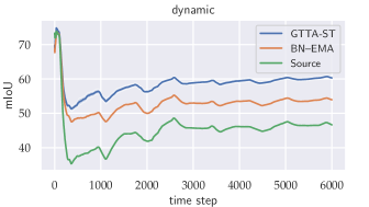
Figure 4: mIoU up to time step $t$ for the dynamic sequence.

Our results are summarized in Table 4. As expected, BN–0 (source) performs the worst by a large margin. While BN–EMA outperforms for all scenarios except highway, BN–0.1 is absolutely $4.4\%$ better than the second best (BN–1) on the highway split. Regarding TENT, we find that the episodic setting performs better than the continual setting. Nevertheless, both variants cannot surpass BN–1. Following X. Wu ., 2021, we evaluate ASM without the attention module and use 4 updates per test sample. For SM-PPM, we get the best results using 8 adaptation steps. SM-PPM performs better than TENT or ASM, however, it is still slightly worse on average compared to BN–EMA. CoTTA does not perform better than BN–1 and performance significantly drops for the longer dynamic sequence. We attribute this to the circumstances that the mean teacher always lags behind the current test domain.

In contrast, our approach GTTA-ST substantially outperforms all baselines by a large margin. Compared to the source model, the mIoU increases by more than $8\%$ in four out of five cases. While self-training alone only provides a clear advantage in two cases, it cannot effectively exploit the gradual domain shift in this setting and even suffers from error accumulation. Style transfer, on the other hand, has a clear advantage in all evaluation settings, since it does not introduce any error accumulation due to label-noise. The combination of both methods now increases the performance on day2night, dynamic, and highway as through the intermediate domain introduced by style transfer, self-training benefits from more reliable pseudo-labels.

In Figure 4, we illustrate the mIoU up to time step $t$ for the dynamic sequence. While the performance of the source model suffers heavily from the domain shift, GTTA-ST is able to maintain good performance throughout the test sequence. Further visualizations and ablation studies are located in Appendix B.

6 Conclusion

In this work we addressed current challenges in online continual and gradual test-time adaptation. Through the creation of intermediate domains by mixup or style transfer, successful self-training for arbitrary domain shifts can be performed. This is supported by experiments for the various gradual changes covered by CarlaTTA and the continual and gradual corruption benchmarks. On all presented benchmarks, we outperform existing methods by a large margin. We are certain that CarlaTTA will give other researchers the opportunity to further investigate the setting of gradual test-time adaptation.

7 Acknowledgments

This publication was created as part of the research project ”KI Delta Learning” (project number: 19A19013R) funded by the Federal Ministry for Economic Affairs and Energy (BMWi) on the basis of a decision by the German Bundestag.

 

Supplementary Materials

 

Appendix A Ablation studies for the classification benchmarks

A.1 Component analysis

Influence of individual components

We begin our ablation studies by examining each component on the continual TTA benchmarks. The results are summarized in Table 5. First, we investigate the effect of solely performing self-training and the advantages of filtering pseudo-labels. Compared to the BN–1 performance, self-training alone only improves the performance on CIFAR10C and CIFAR100C. For ImageNet-C and ImageNet-R, we experience error accumulation resulting in a drastic performance degredation on ImageNet-C. Filtering pseudo-labels according to our proposed threshold benefits all continual classification benchmarks surpassing the BN–1 performance. This is expected since less confident predictions are more likely to be incorrect and can significantly contribute to error accumulation due to large gradient magnitudes Mummadi . (2021). Utilizing source data in the form of source replay stabilizes online test-time adaptation in the sense that the performance is improved on all investigated datasets. We also analyze source replay for TENT D. Wang . (2020) and find that it is also beneficial for methods based on entropy minimization. TENT-continual with source replay achieves an error rate of 18.1%, 31.2%, 61.3%, and 57.6% on CIFAR10C, CIFAR100C, ImageNet-C, and ImageNet-R, respectively. This corresponds to an error reduction of -2.6%, -29.7%, -1.3%, and -1.0%. Especially for CIFAR100C, this is a significant improvement, as TENT-continual without source replay suffers from heavy error accumulation. Last but not least we look into the effect of omitting self-training and solely doing mixup or style transfer. While training on the intermediate domains provided either by mixup or style transfer significantly improves the performance upon BN–1, both methods are limited in mitigating the domain gap. Adding self-training to the framework further benefits the results. This highlights that self-training can have a big performance improvement when provided with reliable pseudo-labels.

Performing multiple update steps

As already shown in Table 1, GTTA-MIX and GTTA-ST benefit from doing multiple update steps. In general, performing multiple updates does not necessarily lead to a performance improvement. Assuming that a proper learning rate for a single update step was chosen, performing, e.g., four updates does not improve the performance when only doing self-training, as presented in Table 5. This especially becomes apparent for ImageNet-C and ImageNet-R, where a drastic performance degradation is experienced. This is not surprising as in the setting of online test-time adaptation only the current test batch $x_{t}^{T}$ is commonly utilized to perform adaptation. We denote this as over-adaptation, where as a result error accumulation can be very prominent. Naturally, filtering less confident predictions, which are more likely to be false predictions, reduces error accumulation. Source replay further helps in the setting of multiple updates to stabilize the adaptation and even results in a performance improvement on CIFAR10C and CIFAR100C compared to a single update. Finally, generating intermediate domains in the form of either mixup or style transfer is the key factor to benefit from multiple updates on CIFAR10C, CIFAR100C, and ImageNet-C. Since mixup has its limitations to create intermediate domains for natural shifts, as imposed by ImageNet-R, only style transfer benefits from multiple updates on this dataset.

Table 5: Component analysis for the continual classification benchmarks. The classification error rate (%) is reported as an average over 5 runs. We investigate the effect of self-training, filtering pseudo-labels, source-replay, and performing mixup and style transfer without self-training (on the right).

	BN–1	self-training		self-training		+ source replay		+ mixup		mixup	style transfer
self-training	n/a	✓		✓		✓		✓		✗	✗
threshold	n/a	✗		✓		✓		✓		n/a	n/a
	-	1	4	1	4	1	4	1	4	1	1
CIFAR10C	20.4	19.9	24.8	18.4	19.4	18.1	17.6	17.2	15.6	17.7	-
CIFAR100C	35.4	33.5	40.6	32.0	33.4	30.5	29.1	30.4	28.9	31.3	-
ImageNet-C	68.6	81.9	97.7	66.6	94.1	65.2	88.9	60.3	57.1	63.1	62.2
ImageNet-R	60.4	61.2	79.6	55.7	67.5	55.4	56.0	56.4	56.6	59.7	56.9

A.2 Trade-off between efficiency and performance

In Table 6 (a) we further explore the effect of performing different numbers of update steps for our overall approaches GTTA-MIX and GTTA-ST, since for some applications it can make sense to neglect computational efficiency in favor of a higher accuracy and vice versa. For GTTA-MIX, CIFAR10C and CIFAR100C benefit increasingly from performing multiple update steps. They show the best performance at 8 update steps reducing the error rate to 15.0% and 28.3%, respectively. For ImageNet-C the best performance is achieved at 6 update steps reducing the error rate from 60.3% for one update to 56.4%. Since mixup shows its difficulties for natural domain shifts, as covered by ImageNet-R, performing more update steps does not necessarily result in a better performance. For GTTA-ST, the best performance for ImageNet-C is again achieved at 6 update steps, resulting in an error rate of 56.3%. In contrast to mixup, style transfer can benefit from multiple update steps for ImageNet-R, achieving the best performance of 52.3% performing 8 update steps.

A.3 Amount of source samples

Since applications can vary in the amount of available memory, we show in Table 6 (b) the error rate for different percentages of saved source samples. While the performance on ImageNet-C and ImageNet-R is only marginally affected by the amount of available source samples for both GTTA-MIX and GTTA-ST, the error rate increases slightly for CIFAR10C and CIFAR100C. Still, using only 10% of the source data does not increase the error rate significantly for both CIFAR10C and CIFAR100C.

Table 6: Classification error rate (%) for different: (a) numbers of update steps; (b) amounts of saved source samples.

(a)	(b)
1 2 4 6 8 GTTA-MIX CIFAR10C 17.2 16.5 15.6 15.2 15.0 CIFAR100C 30.4 29.7 28.9 28.6 28.3 ImageNet-C 60.3 58.4 57.1 56.4 56.6 ImageNet-R 56.4 55.9 56.6 56.1 57.3 GTTA-ST ImageNet-C 59.7 58.0 57.0 56.3 57.0 ImageNet-R 53.8 52.9 52.5 52.9 52.3	100 50 25 10 5 1 CIFAR10C 17.2 17.2 17.2 17.4 17.8 18.8 CIFAR100C 30.4 30.4 30.5 30.6 30.9 32.0 ImageNet-C 60.3 60.0 60.4 60.3 60.3 60.5 ImageNet-R 56.4 56.4 56.1 56.3 55.9 56.5 ImageNet-C 59.7 59.6 59.7 59.7 59.5 59.8 ImageNet-R 53.8 54.1 54.0 54.1 54.5 54.0

A.4 Mixup strength

In Table 7 we investigate the effect of mixup, in particular, how much source or test image is taken into account to create intermediate samples. First, it can be seen that mixup is beneficial for all datasets. ImageNet-R plays a special role in the sense that only a small mixup strength $\lambda_{\text{mix}}=0.1$ marginally improves upon source replay, which corresponds to a mixup strength of $\lambda_{\text{mix}}=0$. For higher mixup strengths, the performance drastically decreases. For CIFAR10C and CIFAR100C $\lambda_{\text{mix}}=1/3$ is a good choice, corresponding to weighting source images twice as strong as test images. ImageNet-C further benefits from higher mixup strength and shows its best performance at $\lambda_{\text{mix}}=0.5$, corresponding to an equal weighting of source and test images.

Table 7: Classification error rate (%) averaged over 5 runs for different mixup strengths $\lambda_{\text{mix}}$. While $\lambda_{\text{mix}}=0$ corresponds to source replay, $\lambda_{\text{mix}}=0.5$ corresponds to the case of equally weighting source and test images.

	0	1/10	1/4	1/3	2/5	1/2
CIFAR10C	18.1	18.1	17.7	17.2	17.4	17.7
CIFAR100C	30.5	30.4	30.4	30.4	30.5	30.6
ImageNet-C	65.2	64.0	61.5	60.3	59.9	59.6
ImageNet-R	55.4	55.2	55.8	56.4	57.1	58.0

A.5 Single sample test-time adaptation

Table 8: Classification error rate (%) for batch size 1 using a sliding window approach with $b$ samples. The weight update is performed once after the complete buffer has changed.

	Time			$t\xrightarrow{\hskip 347.12354pt}$
	Method	batch size	buffer size	Gaussian	shot	impulse	defocus	glass	motion	zoom	snow	frost	fog	brightness	contrast	elastic_trans	pixelate	jpeg	Mean
CIFAR10C	BN–0 (src.)	1	-	72.3	65.7	72.9	46.9	54.3	34.8	42.0	25.1	41.3	26.0	9.3	46.7	26.6	58.5	30.3	43.5
	BN–1	1	16	30.8	28.8	39.2	15.7	37.5	16.8	15.0	20.3	20.2	17.8	10.7	15.5	27.1	23.0	29.9	23.2
	BN–1	1	32	29.3	27.3	37.7	14.2	36.5	15.4	13.8	19.0	18.8	16.8	9.4	14.3	25.2	21.4	28.8	21.9
	GTTA-MIX	1	16	26.5	21.5	28.9	12.7	30.5	13.9	12.9	16.8	15.0	13.1	9.2	10.6	23.0	17.5	22.9	18.3
	GTTA-MIX	1	32	25.5	21.4	28.2	11.9	30.1	13.2	11.9	15.8	14.8	12.8	8.6	10.6	21.4	16.5	23.0	17.7
	GTTA-MIX	200	-	26.0	21.5	29.7	11.1	30.0	12.2	10.5	15.1	14.1	12.3	7.5	10.0	20.4	15.8	21.4	17.2
CIFAR100C	BN–0 (src.)	1	-	73.0	68.0	39.4	29.3	54.1	30.8	28.8	39.5	45.8	50.3	29.5	55.1	37.2	74.7	41.2	46.4
	BN–1	1	16	46.2	44.5	47.1	31.4	46.5	33.3	31.7	39.2	38.6	45.4	30.8	34.7	40.6	37.5	45.2	39.5
	BN–1	1	32	44.1	42.4	45.2	29.6	43.6	31.0	30.0	37.1	36.7	43.8	28.7	32.6	38.0	35.3	42.9	37.4
	GTTA-MIX	1	16	40.1	36.1	37.8	28.3	40.4	29.8	28.3	32.7	31.1	34.2	26.2	27.5	33.5	30.4	38.2	33.0
	GTTA-MIX	1	32	38.9	35.0	36.8	26.6	38.3	28.0	26.5	31.2	30.1	34.0	24.4	26.2	32.1	28.6	36.4	31.5
	GTTA-MIX	200	-	39.4	34.4	36.6	24.7	36.8	26.6	24.3	30.1	28.9	34.6	22.8	25.1	30.7	26.9	34.7	30.4
ImageNet-C	BN–0 (src.)	1	-	95.3	94.6	95.3	84.9	91.1	86.9	77.2	84.4	79.7	77.3	44.4	95.6	85.2	76.9	66.7	82.4
	BN–1	1	16	86.6	85.2	86.0	86.6	86.5	75.7	65.1	67.8	70.5	55.2	37.8	84.6	59.1	55.0	63.7	71.0
	BN–1	1	32	85.4	84.0	84.9	85.6	85.0	74.1	61.9	66.8	68.4	52.6	36.1	83.9	57.1	52.3	61.7	69.3
	GTTA-MIX	1	16	80.8	73.8	71.6	79.3	79.3	70.0	61.1	58.1	59.8	47.6	37.5	73.8	54.2	51.1	53.3	63.4
	GTTA-MIX	1	32	79.8	73.4	70.7	77.3	76.0	64.6	55.8	57.4	58.5	45.5	34.4	67.1	50.5	45.7	49.4	60.4
	GTTA-MIX	64	-	80.5	74.7	72.4	77.8	75.7	64.3	54.0	57.0	58.6	44.6	33.9	67.5	49.4	44.7	49.3	60.3
	GTTA-ST	1	16	80.9	74.3	74.7	77.7	77.3	66.3	58.2	59.0	60.4	47.6	37.6	62.9	53.5	48.8	52.6	62.1
	GTTA-ST	1	32	80.5	74.4	74.0	77.3	74.8	63.5	54.3	56.4	57.6	45.2	33.5	61.8	50.0	45.7	50.7	60.0
	GTTA-ST	64	-	80.6	74.1	74.3	76.8	74.9	62.3	53.9	56.4	58.0	44.1	33.4	62.2	48.6	44.9	50.4	59.7

So far, we only considered the batch setting for the classification task. For some applications, timeliness can be critical, e.g., in autonomous driving, and production data arrives individually rather than in batches. Simply performing prediction and adaptation for a single sample for classification imposes some challenges. First, computing a good estimate of the batch normalization statistics is impossible and second, gradient updates are very noisy. One straightforward approach to overcome these challenges is to save recent data in a buffer and use a sliding window for performing prediction and adaptation. Specifically, we save the last $b$ test samples in a buffer and update the model every $b$ samples due to the strong correlation introduced by the buffer. For current test sample $x_{ti}^{T}$ at time step $t$, the sample is first added to the buffer replacing the oldest sample. Now, the whole buffer is forwarded to make a prediction for the current sample $x_{ti}^{T}$. Needless to say, this comes with a computational overhead, but allows a good estimate of the batch normalization statistics and better gradient updates.

Table 8 illustrates the results for the previously described setting on the continual corruption benchmarks using a buffer of size 16. Due to the much smaller batch size used in this setting, the performance of the baseline BN–1 slightly degrades, since the estimation of the batch statistics becomes more noisy. While the performance of our approach is also slightly worse compared to the results achieved in the batch setting of TTA, GTTA in the single-sample setting still performs on par with most state-of-the-art methods in the batch setting. Using a larger buffer size of 32 further increases the performance. On ImageNet-C the performance in the single sample setting is now comparable with the batch setting, being only 0.1% and 0.3% behind for GTTA-MIX and GTTA-ST, respectively.

Table 9: Investigation of the amount of gradual shift. $\Delta t$ corresponds to the delta time used for all our standard sequences. We report the mIoU (%) for the least common multiple, averaged over 5 runs. For comparison, BN–0 and BN–1 achieve 58.3 and 61.7 on the day2night split and 39.4 and 49.1 on the dynamic split, respectively.

	$4\Delta t$	$2\Delta t$	$\Delta t$	$\Delta t/2$	$\Delta t/4$
day2night	64.6	66.1	66.7	67.2	67.7
dynamic	53.0	55.2	55.6	57.0	56.3

Table 10: Mean intersection-over-union averaged over 5 runs for a) when no domain shift occurs and the test domain is equal to the source domain; b) the domain changes abruptly from day to night.

(a)	(b)
Method BN–0 BN–0.1 BN–1 BN–EMA GTTA-ST 78.4 78.4 76.6 77.6 77.9$\pm$0.14	Method BN–0 BN–0.1 BN–1 BN–EMA GTTA-ST 43.8 52.3 52.8 54.3 59.7$\pm$0.32

Appendix B Ablation studies for CarlaTTA

B.1 Gradual shifts for CarlaTTA

Denoting $\Delta t$ as a proxy for the gradual shift, we generate a dynamic and a day2night sequence which allow to further study the benefits of gradual TTA. By sub-sampling the sequences, we achieve varying degrees of gradual shift. For comparison, we evaluate on the least common multiple. As shown in Table 9 we further benefit from a slower gradual domain shift ($\Delta t/2$), gaining another 0.5% on day2night and 1.4% on dynamic. Having a faster domain shift corresponding to a bigger delta ($2\Delta t$, $4\Delta t$) leads to a reduced performance, indicating that exploiting small gradual shifts is indeed beneficial for our self-training setup. Considering the dynamic sequence, for very small shifts ($\Delta t/4$) we can see a slight performance degradation in comparison to $\Delta t/2$, however, the mIoU is still 0.7% better than $\Delta t$.

B.2 Investigating abrupt shifts and no shifts for CarlaTTA

Since we do not have gradual shifts all the time in the real world, we investigate two additional settings: (a) no domain shift occurs, i.e., the test domain is equal to the source domain and (b) the domain changes abruptly. The results are reported in Table 10 (a) and (b). For the setting of (a), where no domain shift occurs, BN–0, as expected, shows the best performance with a mIoU of 78.4%. Updating the batch statistics through an exponential moving average, i.e., considering BN–EMA, leads to a performance decrease of 0.8%. As a result, also GTTA-ST’s performance cannot achieve BN–0. BN–1 performs even worse at a mIoU of 76.6% illustrating that even in the setting of segmentation in an urban scene a perfect estimation of the batch normalization statistics is not possible for a single sample. For the investigation how GTTA-ST handles abrupt shifts, instead of starting at the first sample of the day2night sequence, we begin after 300 samples, corresponding to a sun altitude of 0°. After one complete night-cycle, the sequence reaches its end. Our method still shows the capability to adapt, reaching a 5.4% higher mIoU than the best BN adaptation approach, namely BN–EMA.

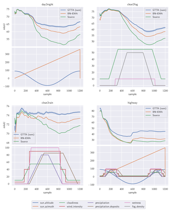
Figure 5: mIoU up to time step $t$ for day2night, clear2fog, clear2rain, and highway. Additionally, we illustrate the progression of the weather parameters to have a direct comparison when a domain shift occurs.

B.3 Performance over time on CarlaTTA

In Figure 5 we illustrate the sequences day2night, clear2fog, clear2rain, and highway and their corresponding progression of environment conditions. At time step $t$ we visualize the mean intersection-over-union averaged from the beginning $t=0$ up to time step $t$. For the day2night sequence a decline in performance can be seen at around sample 300, corresponding to the sun setting. In the setting clear2fog the increase in cloudiness does not influence the model’s performance much. With the fog density increasing, a steady decrease in performance can be seen. For clear2rain the performance of GTTA-ST stays more or less constant, while the source performance steadily decreases with the start of the rain. The highway sequence experiences the same weather behaviour as the dynamic sequence, but additionally experiences a shift of urban scenery to a highway scene. As a result, the performance decreases drastically in the beginning. At around sample 550 an increase in performance can be experienced. This is due to the car driving back into the city, leaving the city again at sample 770.

Appendix C Dataset: CarlaTTA

In the following, we will discuss the specifics about our dataset CarlaTTA. For the generation, CARLA 0.9.13 was used. The data is recorded using an RGB camera and a corresponding semantic segmentation sensor with a resolution of $1920\times 1024$ and a field of view of 40°. Both sensors are positioned 0.5 m forward and 1.2 m upward relative to the ego-vehicle. 14 classes are considered. We visualize the class priors for all sequences in Figure 8.

clear

Table 11: clear weather parameters and maximum values used for rain and fog in the settings clear2rain and clear2fog, respectively.

	sun				rain			fog
	altitude	azimuth	cloudiness	wind	precipitation	deposits	wetness	density	distance	falloff
unit	°	°	%	%	%	%	%	%	m	-
clear	90	0	10	5	0	0	0	0	0	0
night (max)	-90	180	-	-	-	-	-	-	-	-
rain (max)	-	-	55	90	80	85	100	-	-	-
fog (max)	-	-	55	90	-	-	10	50	0	0.9

The source dataset clear is the basis for the four domain changes: day2night, clear2fog, clear2rain, and dynamic. The data for clear is recorded in Town10HD due to being the only town in CARLA with high resolution textures. To increase diversity we generate multiple sequences using different seeds. Specifically, for each seed, up to 40 vehicles and 20 pedestrians are randomly sampled from all (safe) blueprints. We end up with 3500 train and 500 test samples. clear is recorded at noon (sun altitude of 90°) with a cloudiness of 10% and a wind intensity of 5%. All weather parameters are fixed in this setting. The complete overview of the weather parameters used for the clear setting is given in Table 11.

day2night, clear2fog, clear2rain, dynamic

Different domain changes are introduced by the sequences day2night, clear2fog, clear2rain, and dynamic. Each sequence starts with the weather parameters of clear and follows the behavior illustrated in Figure 6. The weather model is based on the implementation of CARLA. The maximum values used for the night, rain, and fog stetting are depicted in Table 11, with a bar indicating no change from the default parameters of clear. While the default sequence length is 1200 samples, dynamic contains 6000 samples to have the capability to study long-term behavior. Figure 7 shows every 100th sample of the mentioned domain shifts.

day2night-slow and dynamic-slow

day2night-slow and dynamic-slow are only considered for the gradual domain shift ablation study. Compared to the regular sequences, where 1200 samples correspond to one complete day-night cycle, in the slow setting, 4800 samples correspond to one day-night cyle. This enables the investigation of smaller domain shifts.

highway

Since Town10HD does not contain any other settings than urban scenery, we use Town04 for the highway sequence. For the corresponding source dataset, we use sequences generated from Town02 (urban setting, similar to Town04) and sequences from Town04 where the ego vehicles only drives in the city. The source dataset contains overall 3000 train and 500 test samples. The highway sequence starts in the city of Town04 and shortly after continues on the highway. It follows the same weather behavior as dynamic. Examples of the sub-sampled sequence are visualized in the last column in Figure 7.

Figure 6: Progression of the weather parameters for the sequences day2night, clear2fog, clear2rain, and dynamic. Note that highway follows the weather behavior of dynamic.

day2night	clear2fog	clear2rain	dynamic	highway

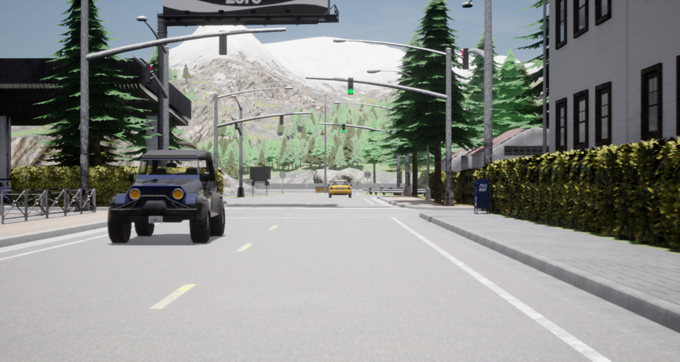
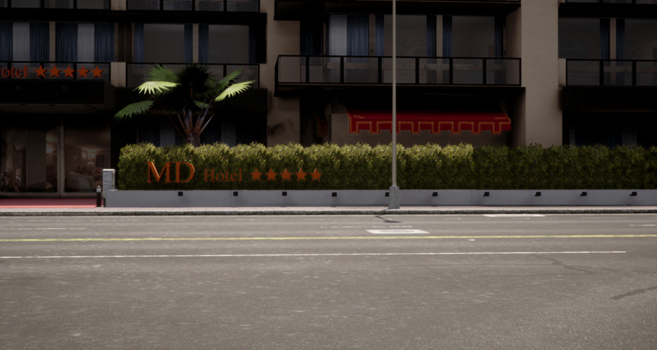
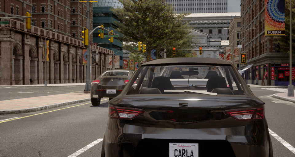
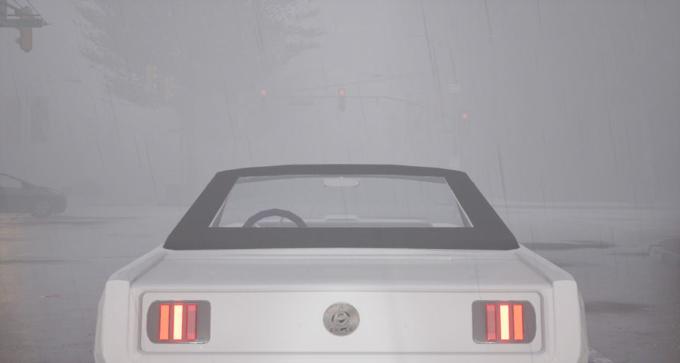
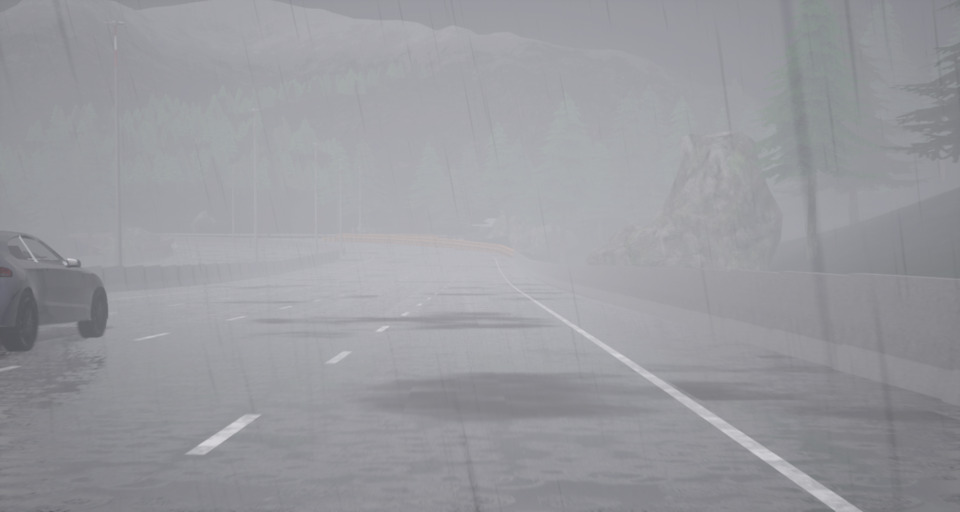
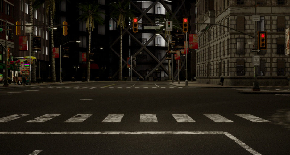
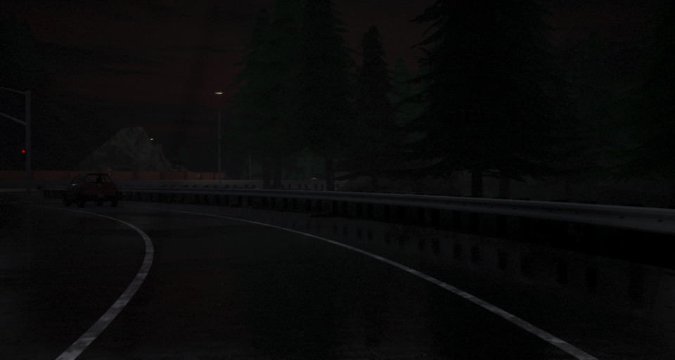
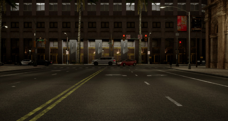
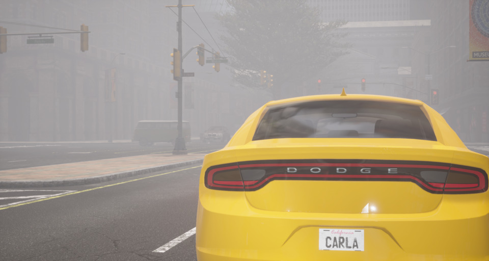
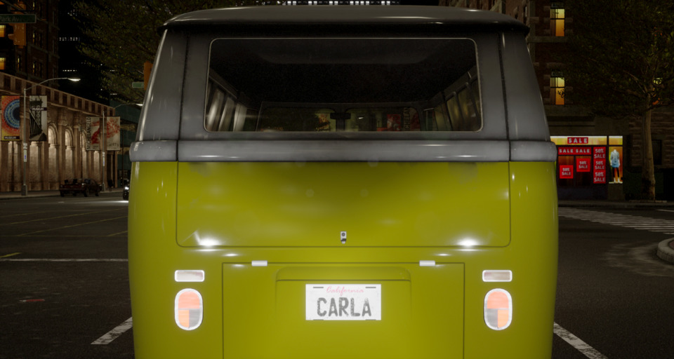
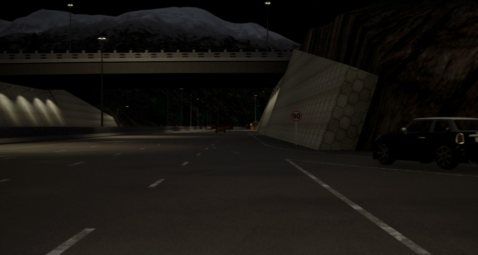
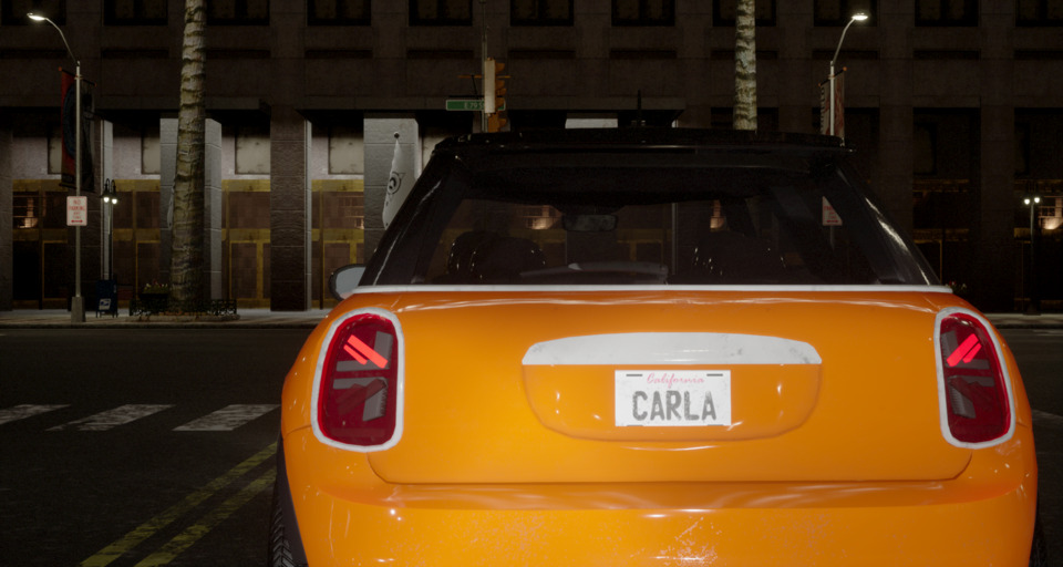
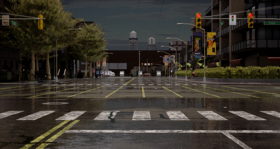
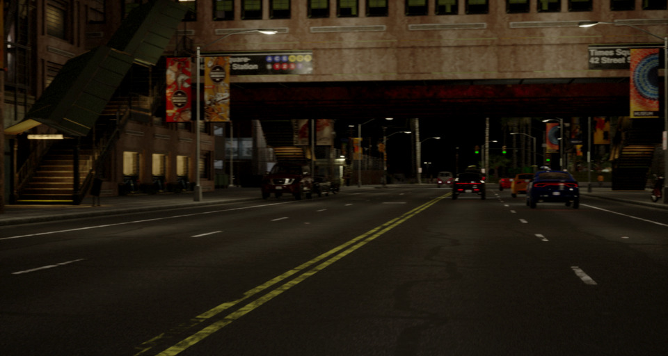
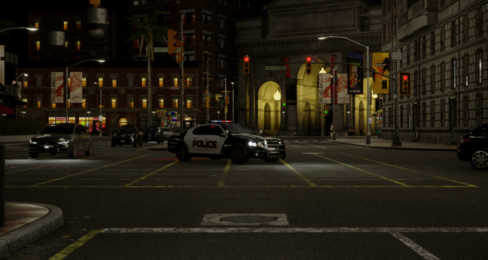
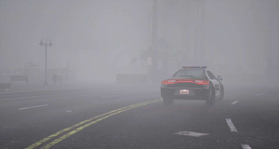
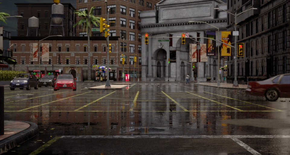
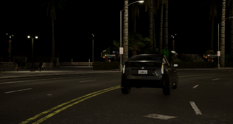
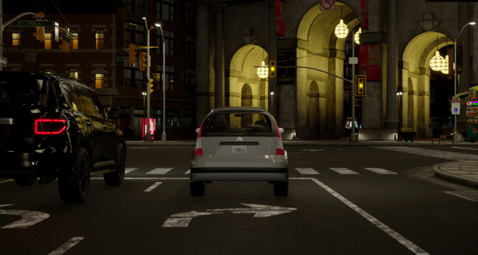
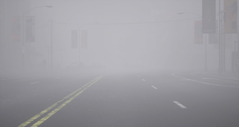
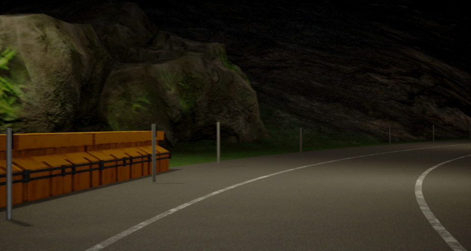
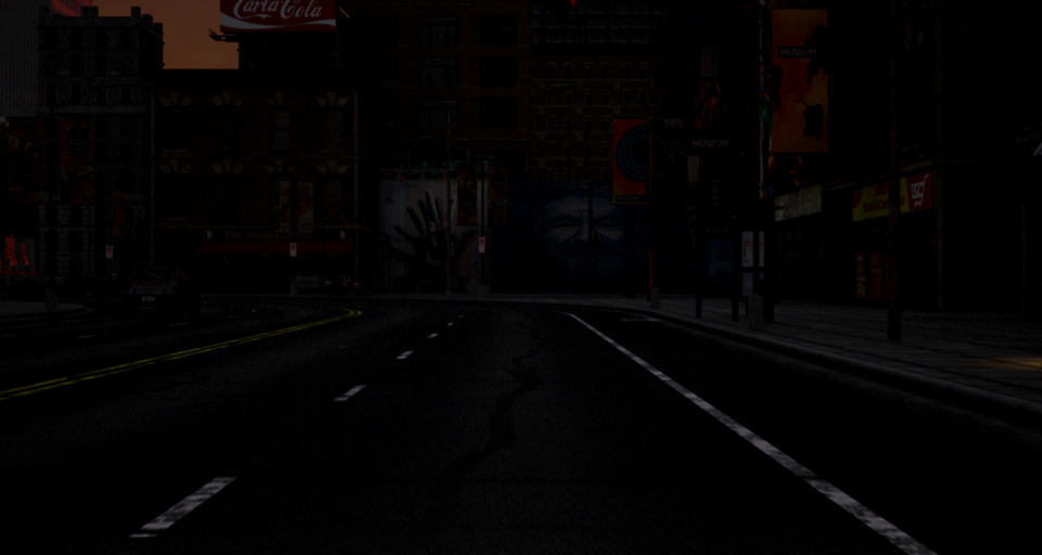
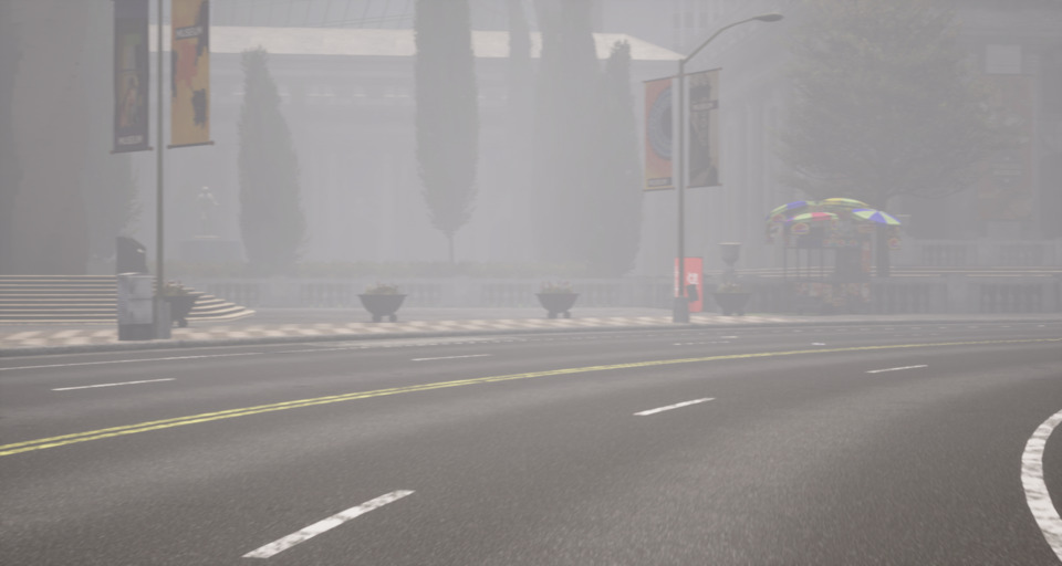
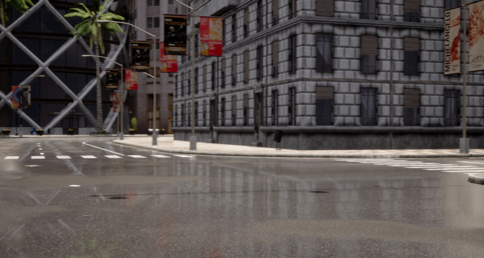
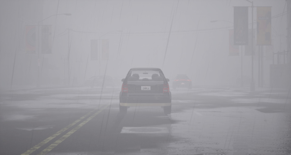
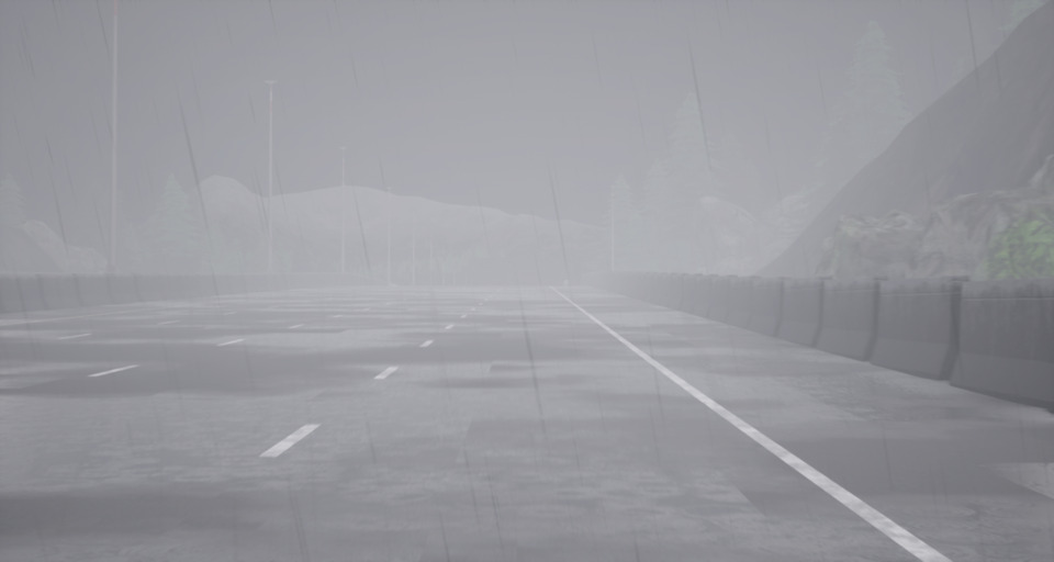
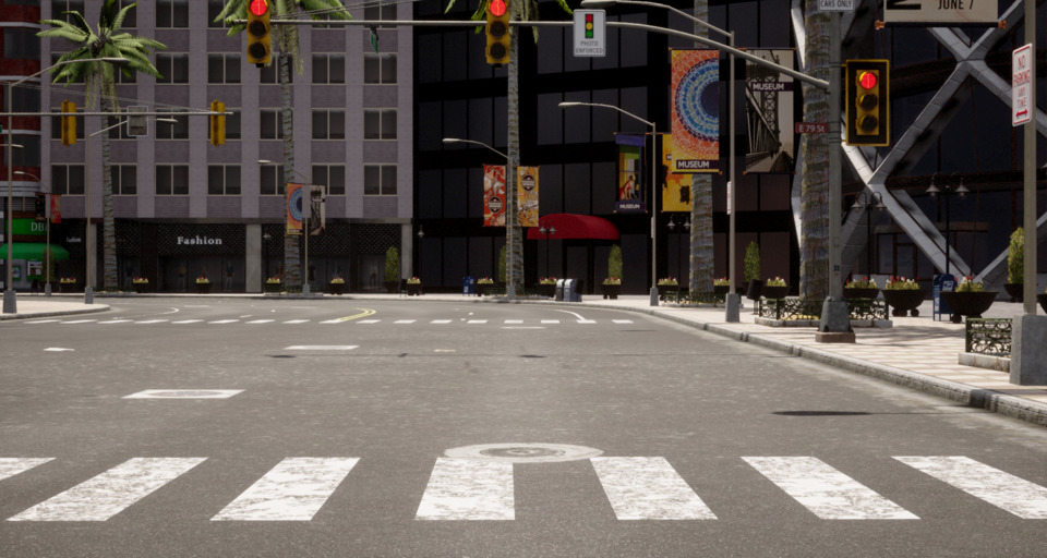
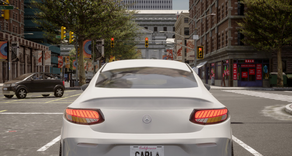
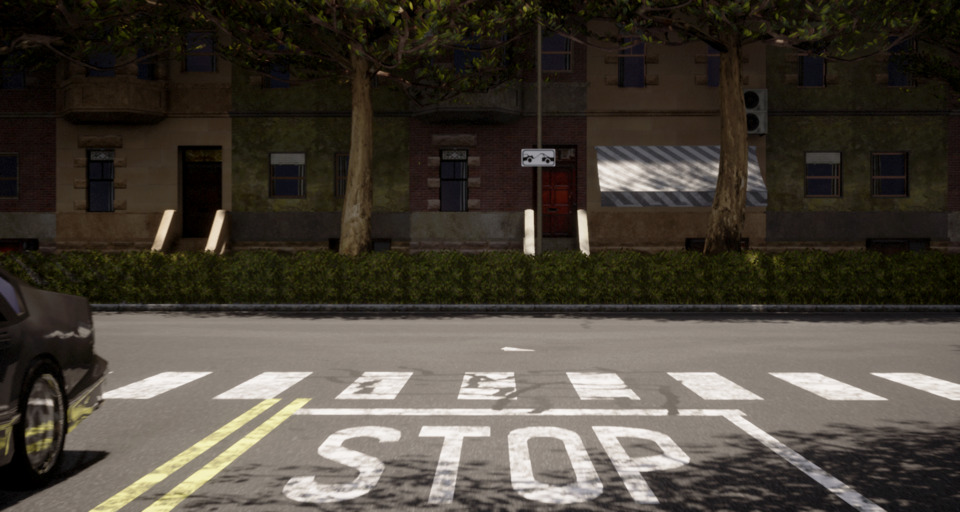
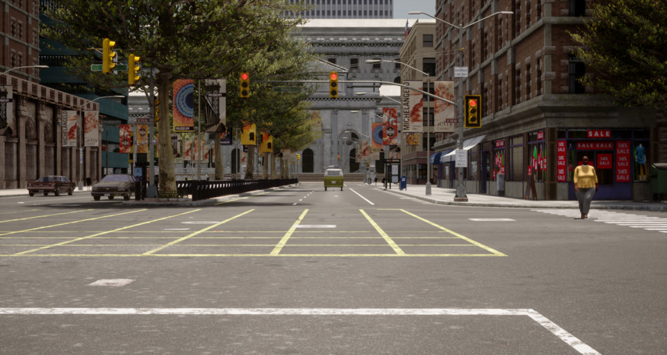
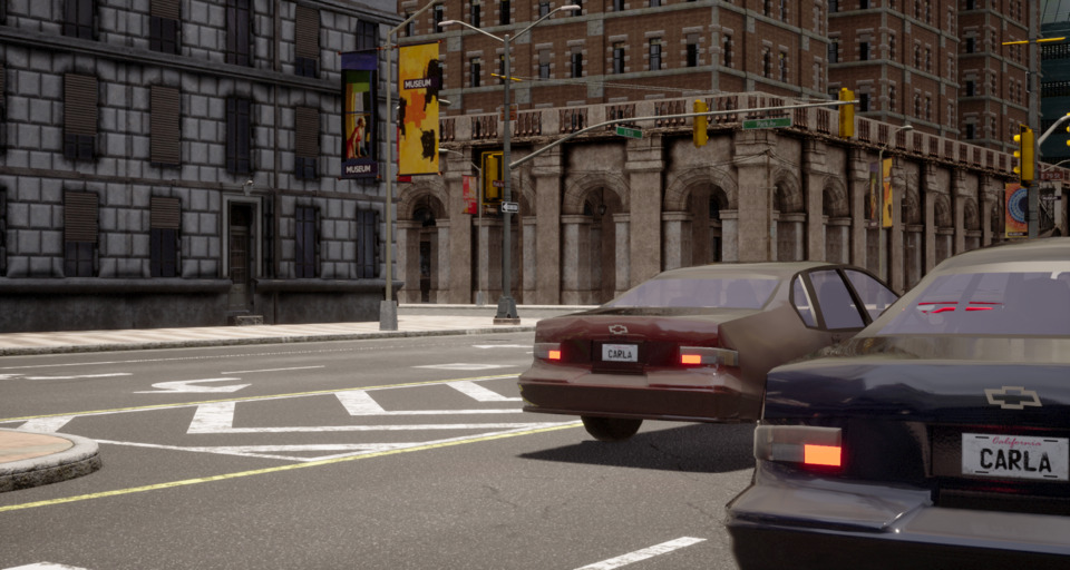
Figure 7: Sequence for the different domain changes. Every 100th example is shown.

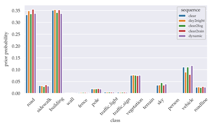
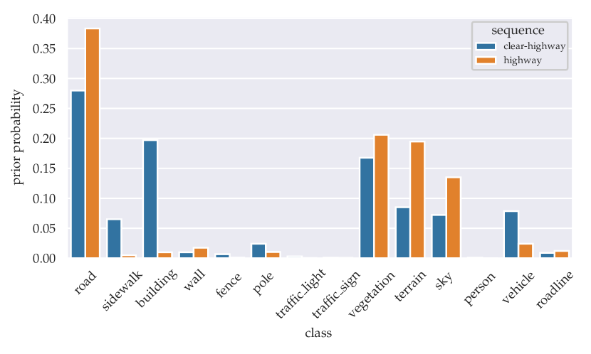
Figure 8: Prior probabilities for the 14 classes. On the top we visualize the prior probabilities corresponding to data originating from Town10HD. On the bottom, we compare clear-highway to highway. The label distribution shift is clearly prominent as the test-time sequence evolves from an urban scenery into a highway setting.

References

- Bartler \BOthers. (\APACyear2022) \APACinsertmetastarMT3{APACrefauthors}Bartler, A., Bühler, A., Wiewel, F., Döbler, M.\BCBL \BBA Yang, B. \APACrefYearMonthDay2022. \BBOQ\APACrefatitleMt3: Meta test-time training for self-supervised test-time adaption Mt3: Meta test-time training for self-supervised test-time adaption.\BBCQ \BIn \APACrefbtitleInternational Conference on Artificial Intelligence and Statistics International conference on artificial intelligence and statistics (\BPGS 3080–3090). \PrintBackRefs\CurrentBib
- Bobu \BOthers. (\APACyear2018) \APACinsertmetastarbobu2018adapting{APACrefauthors}Bobu, A., Tzeng, E., Hoffman, J.\BCBL \BBA Darrell, T. \APACrefYearMonthDay2018. \BBOQ\APACrefatitleAdapting to continuously shifting domains Adapting to continuously shifting domains.\BBCQ \PrintBackRefs\CurrentBib
- D. Chen \BOthers. (\APACyear2022) \APACinsertmetastarchen2022contrastive{APACrefauthors}Chen, D., Wang, D., Darrell, T.\BCBL \BBA Ebrahimi, S. \APACrefYearMonthDay2022. \BBOQ\APACrefatitleContrastive Test-time Adaptation Contrastive test-time adaptation.\BBCQ \BIn \APACrefbtitleCVPR. Cvpr. \PrintBackRefs\CurrentBib
- H\BHBIY. Chen \BBA Chao (\APACyear2021) \APACinsertmetastarIDOL{APACrefauthors}Chen, H\BHBIY.\BCBT \BBA Chao, W\BHBIL. \APACrefYearMonthDay2021. \BBOQ\APACrefatitleGradual Domain Adaptation without Indexed Intermediate Domains Gradual domain adaptation without indexed intermediate domains.\BBCQ \APACjournalVolNumPagesAdvances in Neural Information Processing Systems34. \PrintBackRefs\CurrentBib
- L\BHBIC. Chen \BOthers. (\APACyear2017) \APACinsertmetastarDeeplabv2{APACrefauthors}Chen, L\BHBIC., Papandreou, G., Kokkinos, I., Murphy, K.\BCBL \BBA Yuille, A\BPBIL. \APACrefYearMonthDay2017. \BBOQ\APACrefatitleDeeplab: Semantic image segmentation with deep convolutional nets, atrous convolution, and fully connected crfs Deeplab: Semantic image segmentation with deep convolutional nets, atrous convolution, and fully connected crfs.\BBCQ \APACjournalVolNumPagesIEEE transactions on pattern analysis and machine intelligence404834–848. \PrintBackRefs\CurrentBib
- Cordts \BOthers. (\APACyear2016) \APACinsertmetastarcordts2016cityscapes{APACrefauthors}Cordts, M., Omran, M., Ramos, S., Rehfeld, T., Enzweiler, M., Benenson, R.\BDBLSchiele, B. \APACrefYearMonthDay2016. \BBOQ\APACrefatitleThe cityscapes dataset for semantic urban scene understanding The cityscapes dataset for semantic urban scene understanding.\BBCQ \BIn \APACrefbtitleProceedings of the IEEE conference on computer vision and pattern recognition Proceedings of the ieee conference on computer vision and pattern recognition (\BPGS 3213–3223). \PrintBackRefs\CurrentBib
- Croce \BOthers. (\APACyear2020) \APACinsertmetastarcroce2020robustbench{APACrefauthors}Croce, F., Andriushchenko, M., Sehwag, V., Debenedetti, E., Flammarion, N., Chiang, M.\BDBLHein, M. \APACrefYearMonthDay2020. \BBOQ\APACrefatitleRobustbench: a standardized adversarial robustness benchmark Robustbench: a standardized adversarial robustness benchmark.\BBCQ \APACjournalVolNumPagesarXiv preprint arXiv:2010.09670. \PrintBackRefs\CurrentBib
- Deng \BOthers. (\APACyear2009) \APACinsertmetastarimagenet_cvpr09{APACrefauthors}Deng, J., Dong, W., Socher, R., Li, L\BHBIJ., Li, K.\BCBL \BBA Fei-Fei, L. \APACrefYearMonthDay2009. \BBOQ\APACrefatitleImageNet: A Large-Scale Hierarchical Image Database ImageNet: A Large-Scale Hierarchical Image Database.\BBCQ \BIn \APACrefbtitleCVPR09. Cvpr09. \PrintBackRefs\CurrentBib
- Dosovitskiy \BOthers. (\APACyear2017) \APACinsertmetastarosovitskiy17carla{APACrefauthors}Dosovitskiy, A., Ros, G., Codevilla, F., Lopez, A.\BCBL \BBA Koltun, V. \APACrefYearMonthDay2017. \BBOQ\APACrefatitleCARLA: An Open Urban Driving Simulator CARLA: An open urban driving simulator.\BBCQ \BIn \APACrefbtitleProceedings of the 1st Annual Conference on Robot Learning Proceedings of the 1st annual conference on robot learning (\BPGS 1–16). \PrintBackRefs\CurrentBib
- Ganin \BBA Lempitsky (\APACyear2015) \APACinsertmetastarDANN{APACrefauthors}Ganin, Y.\BCBT \BBA Lempitsky, V. \APACrefYearMonthDay2015. \BBOQ\APACrefatitleUnsupervised domain adaptation by backpropagation Unsupervised domain adaptation by backpropagation.\BBCQ \BIn \APACrefbtitleInternational conference on machine learning International conference on machine learning (\BPGS 1180–1189). \PrintBackRefs\CurrentBib
- Hendrycks \BOthers. (\APACyear2021) \APACinsertmetastarhendrycks2021many{APACrefauthors}Hendrycks, D., Basart, S., Mu, N., Kadavath, S., Wang, F., Dorundo, E.\BDBLothers \APACrefYearMonthDay2021. \BBOQ\APACrefatitleThe many faces of robustness: A critical analysis of out-of-distribution generalization The many faces of robustness: A critical analysis of out-of-distribution generalization.\BBCQ \BIn \APACrefbtitleProceedings of the IEEE/CVF International Conference on Computer Vision Proceedings of the ieee/cvf international conference on computer vision (\BPGS 8340–8349). \PrintBackRefs\CurrentBib
- Hendrycks \BBA Dietterich (\APACyear2019) \APACinsertmetastarhendrycks2019benchmarking{APACrefauthors}Hendrycks, D.\BCBT \BBA Dietterich, T. \APACrefYearMonthDay2019. \BBOQ\APACrefatitleBenchmarking neural network robustness to common corruptions and perturbations Benchmarking neural network robustness to common corruptions and perturbations.\BBCQ \APACjournalVolNumPagesarXiv preprint arXiv:1903.12261. \PrintBackRefs\CurrentBib
- Hendrycks \BOthers. (\APACyear2019) \APACinsertmetastarhendrycks2019augmix{APACrefauthors}Hendrycks, D., Mu, N., Cubuk, E\BPBID., Zoph, B., Gilmer, J.\BCBL \BBA Lakshminarayanan, B. \APACrefYearMonthDay2019. \BBOQ\APACrefatitleAugmix: A simple data processing method to improve robustness and uncertainty Augmix: A simple data processing method to improve robustness and uncertainty.\BBCQ \APACjournalVolNumPagesarXiv preprint arXiv:1912.02781. \PrintBackRefs\CurrentBib
- Hoffman \BOthers. (\APACyear2014) \APACinsertmetastarhoffman14{APACrefauthors}Hoffman, J., Darrell, T.\BCBL \BBA Saenko, K. \APACrefYearMonthDay2014. \BBOQ\APACrefatitleContinuous manifold based adaptation for evolving visual domains Continuous manifold based adaptation for evolving visual domains.\BBCQ \BIn \APACrefbtitleProceedings of the IEEE Conference on Computer Vision and Pattern Recognition Proceedings of the ieee conference on computer vision and pattern recognition (\BPGS 867–874). \PrintBackRefs\CurrentBib
- Hoffman \BOthers. (\APACyear2018) \APACinsertmetastarCYCADA{APACrefauthors}Hoffman, J., Tzeng, E., Park, T., Zhu, J\BHBIY., Isola, P., Saenko, K.\BDBLDarrell, T. \APACrefYearMonthDay2018. \BBOQ\APACrefatitleCycada: Cycle-consistent adversarial domain adaptation Cycada: Cycle-consistent adversarial domain adaptation.\BBCQ \BIn \APACrefbtitleInternational conference on machine learning International conference on machine learning (\BPGS 1989–1998). \PrintBackRefs\CurrentBib
- Hoyer \BOthers. (\APACyear2022) \APACinsertmetastarhoyer2022daformer{APACrefauthors}Hoyer, L., Dai, D.\BCBL \BBA Van Gool, L. \APACrefYearMonthDay2022. \BBOQ\APACrefatitleDaformer: Improving network architectures and training strategies for domain-adaptive semantic segmentation Daformer: Improving network architectures and training strategies for domain-adaptive semantic segmentation.\BBCQ \BIn \APACrefbtitleProceedings of the IEEE/CVF Conference on Computer Vision and Pattern Recognition Proceedings of the ieee/cvf conference on computer vision and pattern recognition (\BPGS 9924–9935). \PrintBackRefs\CurrentBib
- Huang \BBA Belongie (\APACyear2017) \APACinsertmetastarAdaIN{APACrefauthors}Huang, X.\BCBT \BBA Belongie, S. \APACrefYearMonthDay2017. \BBOQ\APACrefatitleArbitrary style transfer in real-time with adaptive instance normalization Arbitrary style transfer in real-time with adaptive instance normalization.\BBCQ \BIn \APACrefbtitleProceedings of the IEEE International Conference on Computer Vision Proceedings of the ieee international conference on computer vision (\BPGS 1501–1510). \PrintBackRefs\CurrentBib
- Isola \BOthers. (\APACyear2017) \APACinsertmetastarisola2017image{APACrefauthors}Isola, P., Zhu, J\BHBIY., Zhou, T.\BCBL \BBA Efros, A\BPBIA. \APACrefYearMonthDay2017. \BBOQ\APACrefatitleImage-to-image translation with conditional adversarial networks Image-to-image translation with conditional adversarial networks.\BBCQ \BIn \APACrefbtitleProceedings of the IEEE conference on computer vision and pattern recognition Proceedings of the ieee conference on computer vision and pattern recognition (\BPGS 1125–1134). \PrintBackRefs\CurrentBib
- Kim \BOthers. (\APACyear2021) \APACinsertmetastarkim2021deep{APACrefauthors}Kim, S., Kim, S.\BCBL \BBA Kim, S. \APACrefYearMonthDay2021. \BBOQ\APACrefatitleDeep Translation Prior: Test-time Training for Photorealistic Style Transfer Deep translation prior: Test-time training for photorealistic style transfer.\BBCQ \APACjournalVolNumPagesarXiv preprint arXiv:2112.06150. \PrintBackRefs\CurrentBib
- Kingma \BBA Ba (\APACyear2014) \APACinsertmetastarkingma2014adam{APACrefauthors}Kingma, D\BPBIP.\BCBT \BBA Ba, J. \APACrefYearMonthDay2014. \BBOQ\APACrefatitleAdam: A method for stochastic optimization Adam: A method for stochastic optimization.\BBCQ \APACjournalVolNumPagesarXiv preprint arXiv:1412.6980. \PrintBackRefs\CurrentBib
- Krizhevsky \BOthers. (\APACyear2009) \APACinsertmetastarkrizhevsky2009learning{APACrefauthors}Krizhevsky, A., Hinton, G.\BCBL \BOthersPeriod. \APACrefYearMonthDay2009. \BBOQ\APACrefatitleLearning multiple layers of features from tiny images Learning multiple layers of features from tiny images.\BBCQ \PrintBackRefs\CurrentBib
- Kumar \BOthers. (\APACyear2020) \APACinsertmetastarkumar2020understanding{APACrefauthors}Kumar, A., Ma, T.\BCBL \BBA Liang, P. \APACrefYearMonthDay2020. \BBOQ\APACrefatitleUnderstanding self-training for gradual domain adaptation Understanding self-training for gradual domain adaptation.\BBCQ \BIn \APACrefbtitleInternational Conference on Machine Learning International conference on machine learning (\BPGS 5468–5479). \PrintBackRefs\CurrentBib
- G. Li \BOthers. (\APACyear2020) \APACinsertmetastarCCM{APACrefauthors}Li, G., Kang, G., Liu, W., Wei, Y.\BCBL \BBA Yang, Y. \APACrefYearMonthDay2020. \BBOQ\APACrefatitleContent-consistent matching for domain adaptive semantic segmentation Content-consistent matching for domain adaptive semantic segmentation.\BBCQ \BIn \APACrefbtitleEuropean Conference on Computer Vision European conference on computer vision (\BPGS 440–456). \PrintBackRefs\CurrentBib
- Y. Li \BOthers. (\APACyear2019) \APACinsertmetastarBidirectional{APACrefauthors}Li, Y., Yuan, L.\BCBL \BBA Vasconcelos, N. \APACrefYearMonthDay2019. \BBOQ\APACrefatitleBidirectional learning for domain adaptation of semantic segmentation Bidirectional learning for domain adaptation of semantic segmentation.\BBCQ \BIn \APACrefbtitleProceedings of the IEEE Conference on Computer Vision and Pattern Recognition Proceedings of the ieee conference on computer vision and pattern recognition (\BPGS 6936–6945). \PrintBackRefs\CurrentBib
- Liang \BOthers. (\APACyear2020) \APACinsertmetastarliang2020we{APACrefauthors}Liang, J., Hu, D.\BCBL \BBA Feng, J. \APACrefYearMonthDay2020. \BBOQ\APACrefatitleDo we really need to access the source data? source hypothesis transfer for unsupervised domain adaptation Do we really need to access the source data? source hypothesis transfer for unsupervised domain adaptation.\BBCQ \BIn \APACrefbtitleInternational Conference on Machine Learning International conference on machine learning (\BPGS 6028–6039). \PrintBackRefs\CurrentBib
- Liu \BOthers. (\APACyear2021) \APACinsertmetastarliu2021ttt++{APACrefauthors}Liu, Y., Kothari, P., van Delft, B., Bellot-Gurlet, B., Mordan, T.\BCBL \BBA Alahi, A. \APACrefYearMonthDay2021. \BBOQ\APACrefatitleTTT++: When Does Self-Supervised Test-Time Training Fail or Thrive? Ttt++: When does self-supervised test-time training fail or thrive?\BBCQ \APACjournalVolNumPagesAdvances in Neural Information Processing Systems34. \PrintBackRefs\CurrentBib
- Luo \BOthers. (\APACyear2020) \APACinsertmetastarASM{APACrefauthors}Luo, Y., Liu, P., Guan, T., Yu, J.\BCBL \BBA Yang, Y. \APACrefYearMonthDay2020. \BBOQ\APACrefatitleAdversarial style mining for one-shot unsupervised domain adaptation Adversarial style mining for one-shot unsupervised domain adaptation.\BBCQ \APACjournalVolNumPagesAdvances in Neural Information Processing Systems3320612–20623. \PrintBackRefs\CurrentBib
- Marsden, Bartler\BCBL \BOthers. (\APACyear2022) \APACinsertmetastarmarsden2022contrastive{APACrefauthors}Marsden, R\BPBIA., Bartler, A., Döbler, M.\BCBL \BBA Yang, B. \APACrefYearMonthDay2022. \BBOQ\APACrefatitleContrastive learning and self-training for unsupervised domain adaptation in semantic segmentation Contrastive learning and self-training for unsupervised domain adaptation in semantic segmentation.\BBCQ \BIn \APACrefbtitle2022 International Joint Conference on Neural Networks (IJCNN) 2022 international joint conference on neural networks (ijcnn) (\BPGS 1–8). \PrintBackRefs\CurrentBib
- Marsden, Wiewel\BCBL \BOthers. (\APACyear2022) \APACinsertmetastarCACE{APACrefauthors}Marsden, R\BPBIA., Wiewel, F., Döbler, M., Yang, Y.\BCBL \BBA Yang, B. \APACrefYearMonthDay2022. \BBOQ\APACrefatitleContinual Unsupervised Domain Adaptation for Semantic Segmentation using a Class-Specific Transfer Continual unsupervised domain adaptation for semantic segmentation using a class-specific transfer.\BBCQ \BIn \APACrefbtitle2022 International Joint Conference on Neural Networks (IJCNN) 2022 international joint conference on neural networks (ijcnn) (\BPGS 1–8). \PrintBackRefs\CurrentBib
- McCloskey \BBA Cohen (\APACyear1989) \APACinsertmetastarmccloskey1989catastrophic{APACrefauthors}McCloskey, M.\BCBT \BBA Cohen, N\BPBIJ. \APACrefYearMonthDay1989. \BBOQ\APACrefatitleCatastrophic interference in connectionist networks: The sequential learning problem Catastrophic interference in connectionist networks: The sequential learning problem.\BBCQ \BIn \APACrefbtitlePsychology of learning and motivation Psychology of learning and motivation (\BVOL 24, \BPGS 109–165). \APACaddressPublisherElsevier. \PrintBackRefs\CurrentBib
- Mei \BOthers. (\APACyear2020) \APACinsertmetastarIAST{APACrefauthors}Mei, K., Zhu, C., Zou, J.\BCBL \BBA Zhang, S. \APACrefYearMonthDay2020. \BBOQ\APACrefatitleInstance adaptive self-training for unsupervised domain adaptation Instance adaptive self-training for unsupervised domain adaptation.\BBCQ \APACjournalVolNumPagesarXiv preprint arXiv:2008.12197. \PrintBackRefs\CurrentBib
- Mintun \BOthers. (\APACyear2021) \APACinsertmetastarmintun2021interaction{APACrefauthors}Mintun, E., Kirillov, A.\BCBL \BBA Xie, S. \APACrefYearMonthDay2021. \BBOQ\APACrefatitleOn interaction between augmentations and corruptions in natural corruption robustness On interaction between augmentations and corruptions in natural corruption robustness.\BBCQ \APACjournalVolNumPagesAdvances in Neural Information Processing Systems34. \PrintBackRefs\CurrentBib
- Muandet \BOthers. (\APACyear2013) \APACinsertmetastarmuandet2013domain{APACrefauthors}Muandet, K., Balduzzi, D.\BCBL \BBA Schölkopf, B. \APACrefYearMonthDay2013. \BBOQ\APACrefatitleDomain generalization via invariant feature representation Domain generalization via invariant feature representation.\BBCQ \BIn \APACrefbtitleInternational Conference on Machine Learning International conference on machine learning (\BPGS 10–18). \PrintBackRefs\CurrentBib
- Mummadi \BOthers. (\APACyear2021) \APACinsertmetastarmummadi2021test{APACrefauthors}Mummadi, C\BPBIK., Hutmacher, R., Rambach, K., Levinkov, E., Brox, T.\BCBL \BBA Metzen, J\BPBIH. \APACrefYearMonthDay2021. \BBOQ\APACrefatitleTest-time adaptation to distribution shift by confidence maximization and input transformation Test-time adaptation to distribution shift by confidence maximization and input transformation.\BBCQ \APACjournalVolNumPagesarXiv preprint arXiv:2106.14999. \PrintBackRefs\CurrentBib
- Quiñonero-Candela \BOthers. (\APACyear2008) \APACinsertmetastarquinonero2008dataset{APACrefauthors}Quiñonero-Candela, J., Sugiyama, M., Schwaighofer, A.\BCBL \BBA Lawrence, N\BPBID. \APACrefYear2008. \APACrefbtitleDataset shift in machine learning Dataset shift in machine learning. \APACaddressPublisherMit Press. \PrintBackRefs\CurrentBib
- Richter \BOthers. (\APACyear2016) \APACinsertmetastarRichter_2016_ECCV{APACrefauthors}Richter, S\BPBIR., Vineet, V., Roth, S.\BCBL \BBA Koltun, V. \APACrefYearMonthDay2016. \BBOQ\APACrefatitlePlaying for Data: Ground Truth from Computer Games Playing for data: Ground truth from computer games.\BBCQ \BIn B. Leibe, J. Matas, N. Sebe\BCBL \BBA M. Welling (\BEDS), \APACrefbtitleEuropean Conference on Computer Vision (ECCV) European conference on computer vision (eccv) (\BVOL 9906, \BPGS 102–118). \APACaddressPublisherSpringer International Publishing. \PrintBackRefs\CurrentBib
- Ros \BOthers. (\APACyear2016) \APACinsertmetastarros2016synthia{APACrefauthors}Ros, G., Sellart, L., Materzynska, J., Vazquez, D.\BCBL \BBA Lopez, A\BPBIM. \APACrefYearMonthDay2016. \BBOQ\APACrefatitleThe synthia dataset: A large collection of synthetic images for semantic segmentation of urban scenes The synthia dataset: A large collection of synthetic images for semantic segmentation of urban scenes.\BBCQ \BIn \APACrefbtitleProceedings of the IEEE conference on computer vision and pattern recognition Proceedings of the ieee conference on computer vision and pattern recognition (\BPGS 3234–3243). \PrintBackRefs\CurrentBib
- Sakaridis \BOthers. (\APACyear2021) \APACinsertmetastarsakaridis2021acdc{APACrefauthors}Sakaridis, C., Dai, D.\BCBL \BBA Van Gool, L. \APACrefYearMonthDay2021. \BBOQ\APACrefatitleACDC: The adverse conditions dataset with correspondences for semantic driving scene understanding Acdc: The adverse conditions dataset with correspondences for semantic driving scene understanding.\BBCQ \BIn \APACrefbtitleProceedings of the IEEE/CVF International Conference on Computer Vision Proceedings of the ieee/cvf international conference on computer vision (\BPGS 10765–10775). \PrintBackRefs\CurrentBib
- Schneider \BOthers. (\APACyear2020) \APACinsertmetastarschneider2020improving{APACrefauthors}Schneider, S., Rusak, E., Eck, L., Bringmann, O., Brendel, W.\BCBL \BBA Bethge, M. \APACrefYearMonthDay2020. \BBOQ\APACrefatitleImproving robustness against common corruptions by covariate shift adaptation Improving robustness against common corruptions by covariate shift adaptation.\BBCQ \APACjournalVolNumPagesAdvances in Neural Information Processing Systems3311539–11551. \PrintBackRefs\CurrentBib
- P. Sun \BOthers. (\APACyear2020) \APACinsertmetastarsun2020scalability{APACrefauthors}Sun, P., Kretzschmar, H., Dotiwalla, X., Chouard, A., Patnaik, V., Tsui, P.\BDBLothers \APACrefYearMonthDay2020. \BBOQ\APACrefatitleScalability in perception for autonomous driving: Waymo open dataset Scalability in perception for autonomous driving: Waymo open dataset.\BBCQ \BIn \APACrefbtitleProceedings of the IEEE/CVF conference on computer vision and pattern recognition Proceedings of the ieee/cvf conference on computer vision and pattern recognition (\BPGS 2446–2454). \PrintBackRefs\CurrentBib
- Y. Sun \BOthers. (\APACyear2020) \APACinsertmetastarTTT{APACrefauthors}Sun, Y., Wang, X., Liu, Z., Miller, J., Efros, A.\BCBL \BBA Hardt, M. \APACrefYearMonthDay2020. \BBOQ\APACrefatitleTest-time training with self-supervision for generalization under distribution shifts Test-time training with self-supervision for generalization under distribution shifts.\BBCQ \BIn \APACrefbtitleInternational Conference on Machine Learning International conference on machine learning (\BPGS 9229–9248). \PrintBackRefs\CurrentBib
- Tobin \BOthers. (\APACyear2017) \APACinsertmetastartobin2017domain{APACrefauthors}Tobin, J., Fong, R., Ray, A., Schneider, J., Zaremba, W.\BCBL \BBA Abbeel, P. \APACrefYearMonthDay2017. \BBOQ\APACrefatitleDomain randomization for transferring deep neural networks from simulation to the real world Domain randomization for transferring deep neural networks from simulation to the real world.\BBCQ \BIn \APACrefbtitle2017 IEEE/RSJ international conference on intelligent robots and systems (IROS) 2017 ieee/rsj international conference on intelligent robots and systems (iros) (\BPGS 23–30). \PrintBackRefs\CurrentBib
- Tranheden \BOthers. (\APACyear2021) \APACinsertmetastarDACS{APACrefauthors}Tranheden, W., Olsson, V., Pinto, J.\BCBL \BBA Svensson, L. \APACrefYearMonthDay2021. \BBOQ\APACrefatitleDACS: Domain Adaptation via Cross-domain Mixed Sampling Dacs: Domain adaptation via cross-domain mixed sampling.\BBCQ \BIn \APACrefbtitleProceedings of the IEEE/CVF Winter Conference on Applications of Computer Vision Proceedings of the ieee/cvf winter conference on applications of computer vision (\BPGS 1379–1389). \PrintBackRefs\CurrentBib
- Tremblay \BOthers. (\APACyear2018) \APACinsertmetastartremblay2018training{APACrefauthors}Tremblay, J., Prakash, A., Acuna, D., Brophy, M., Jampani, V., Anil, C.\BDBLBirchfield, S. \APACrefYearMonthDay2018. \BBOQ\APACrefatitleTraining deep networks with synthetic data: Bridging the reality gap by domain randomization Training deep networks with synthetic data: Bridging the reality gap by domain randomization.\BBCQ \BIn \APACrefbtitleProceedings of the IEEE conference on computer vision and pattern recognition workshops Proceedings of the ieee conference on computer vision and pattern recognition workshops (\BPGS 969–977). \PrintBackRefs\CurrentBib
- Tsai \BOthers. (\APACyear2018) \APACinsertmetastarAdaptSegNet{APACrefauthors}Tsai, Y\BHBIH., Hung, W\BHBIC., Schulter, S., Sohn, K., Yang, M\BHBIH.\BCBL \BBA Chandraker, M. \APACrefYearMonthDay2018. \BBOQ\APACrefatitleLearning to adapt structured output space for semantic segmentation Learning to adapt structured output space for semantic segmentation.\BBCQ \BIn \APACrefbtitleProceedings of the IEEE Conference on Computer Vision and Pattern Recognition Proceedings of the ieee conference on computer vision and pattern recognition (\BPGS 7472–7481). \PrintBackRefs\CurrentBib
- Tsai \BOthers. (\APACyear2019) \APACinsertmetastarPatchAlign{APACrefauthors}Tsai, Y\BHBIH., Sohn, K., Schulter, S.\BCBL \BBA Chandraker, M. \APACrefYearMonthDay2019. \BBOQ\APACrefatitleDomain adaptation for structured output via discriminative patch representations Domain adaptation for structured output via discriminative patch representations.\BBCQ \BIn \APACrefbtitleProceedings of the IEEE International Conference on Computer Vision Proceedings of the ieee international conference on computer vision (\BPGS 1456–1465). \PrintBackRefs\CurrentBib
- Vergara \BOthers. (\APACyear2012) \APACinsertmetastarvergara2012chemical{APACrefauthors}Vergara, A., Vembu, S., Ayhan, T., Ryan, M\BPBIA., Homer, M\BPBIL.\BCBL \BBA Huerta, R. \APACrefYearMonthDay2012. \BBOQ\APACrefatitleChemical gas sensor drift compensation using classifier ensembles Chemical gas sensor drift compensation using classifier ensembles.\BBCQ \APACjournalVolNumPagesSensors and Actuators B: Chemical166320–329. \PrintBackRefs\CurrentBib
- Vu \BOthers. (\APACyear2019) \APACinsertmetastarADVENT{APACrefauthors}Vu, T\BHBIH., Jain, H., Bucher, M., Cord, M.\BCBL \BBA Pérez, P. \APACrefYearMonthDay2019. \BBOQ\APACrefatitleAdvent: Adversarial entropy minimization for domain adaptation in semantic segmentation Advent: Adversarial entropy minimization for domain adaptation in semantic segmentation.\BBCQ \BIn \APACrefbtitleProceedings of the IEEE conference on computer vision and pattern recognition Proceedings of the ieee conference on computer vision and pattern recognition (\BPGS 2517–2526). \PrintBackRefs\CurrentBib
- D. Wang \BOthers. (\APACyear2020) \APACinsertmetastarTENT{APACrefauthors}Wang, D., Shelhamer, E., Liu, S., Olshausen, B.\BCBL \BBA Darrell, T. \APACrefYearMonthDay2020. \BBOQ\APACrefatitleTent: Fully test-time adaptation by entropy minimization Tent: Fully test-time adaptation by entropy minimization.\BBCQ \APACjournalVolNumPagesarXiv preprint arXiv:2006.10726. \PrintBackRefs\CurrentBib
- Q. Wang \BOthers. (\APACyear2022) \APACinsertmetastarwang2022continual{APACrefauthors}Wang, Q., Fink, O., Van Gool, L.\BCBL \BBA Dai, D. \APACrefYearMonthDay2022. \BBOQ\APACrefatitleContinual test-time domain adaptation Continual test-time domain adaptation.\BBCQ \BIn \APACrefbtitleProceedings of the IEEE/CVF Conference on Computer Vision and Pattern Recognition Proceedings of the ieee/cvf conference on computer vision and pattern recognition (\BPGS 7201–7211). \PrintBackRefs\CurrentBib
- X. Wu \BOthers. (\APACyear2021) \APACinsertmetastarSM-PPM{APACrefauthors}Wu, X., Wu, Z., Lu, Y., Ju, L.\BCBL \BBA Wang, S. \APACrefYearMonthDay2021. \BBOQ\APACrefatitleStyle Mixing and Patchwise Prototypical Matching for One-Shot Unsupervised Domain Adaptive Semantic Segmentation Style mixing and patchwise prototypical matching for one-shot unsupervised domain adaptive semantic segmentation.\BBCQ \APACjournalVolNumPagesarXiv preprint arXiv:2112.04665. \PrintBackRefs\CurrentBib
- Z. Wu \BOthers. (\APACyear2019) \APACinsertmetastarACE{APACrefauthors}Wu, Z., Wang, X., Gonzalez, J\BPBIE., Goldstein, T.\BCBL \BBA Davis, L\BPBIS. \APACrefYearMonthDay2019. \BBOQ\APACrefatitleACE: adapting to changing environments for semantic segmentation Ace: adapting to changing environments for semantic segmentation.\BBCQ \BIn \APACrefbtitleProceedings of the IEEE International Conference on Computer Vision Proceedings of the ieee international conference on computer vision (\BPGS 2121–2130). \PrintBackRefs\CurrentBib
- Wulfmeier \BOthers. (\APACyear2018) \APACinsertmetastarwulfmeier{APACrefauthors}Wulfmeier, M., Bewley, A.\BCBL \BBA Posner, I. \APACrefYearMonthDay2018. \BBOQ\APACrefatitleIncremental adversarial domain adaptation for continually changing environments Incremental adversarial domain adaptation for continually changing environments.\BBCQ \BIn \APACrefbtitle2018 IEEE International conference on robotics and automation (ICRA) 2018 ieee international conference on robotics and automation (icra) (\BPGS 4489–4495). \PrintBackRefs\CurrentBib
- Yang \BBA Soatto (\APACyear2020) \APACinsertmetastarFDA{APACrefauthors}Yang, Y.\BCBT \BBA Soatto, S. \APACrefYearMonthDay2020. \BBOQ\APACrefatitleFda: Fourier domain adaptation for semantic segmentation Fda: Fourier domain adaptation for semantic segmentation.\BBCQ \BIn \APACrefbtitleProceedings of the IEEE/CVF Conference on Computer Vision and Pattern Recognition Proceedings of the ieee/cvf conference on computer vision and pattern recognition (\BPGS 4085–4095). \PrintBackRefs\CurrentBib
- Yu \BOthers. (\APACyear2020) \APACinsertmetastaryu2020bdd100k{APACrefauthors}Yu, F., Chen, H., Wang, X., Xian, W., Chen, Y., Liu, F.\BDBLDarrell, T. \APACrefYearMonthDay2020. \BBOQ\APACrefatitleBdd100k: A diverse driving dataset for heterogeneous multitask learning Bdd100k: A diverse driving dataset for heterogeneous multitask learning.\BBCQ \BIn \APACrefbtitleProceedings of the IEEE/CVF conference on computer vision and pattern recognition Proceedings of the ieee/cvf conference on computer vision and pattern recognition (\BPGS 2636–2645). \PrintBackRefs\CurrentBib
- H. Zhang \BOthers. (\APACyear2017) \APACinsertmetastarzhang2017mixup{APACrefauthors}Zhang, H., Cisse, M., Dauphin, Y\BPBIN.\BCBL \BBA Lopez-Paz, D. \APACrefYearMonthDay2017. \BBOQ\APACrefatitlemixup: Beyond empirical risk minimization mixup: Beyond empirical risk minimization.\BBCQ \APACjournalVolNumPagesarXiv preprint arXiv:1710.09412. \PrintBackRefs\CurrentBib
- M. Zhang \BOthers. (\APACyear2021) \APACinsertmetastarMEMO{APACrefauthors}Zhang, M., Levine, S.\BCBL \BBA Finn, C. \APACrefYearMonthDay2021. \BBOQ\APACrefatitleMEMO: Test Time Robustness via Adaptation and Augmentation Memo: Test time robustness via adaptation and augmentation.\BBCQ \APACjournalVolNumPagesarXiv preprint arXiv:2110.09506. \PrintBackRefs\CurrentBib
- P. Zhang \BOthers. (\APACyear2021) \APACinsertmetastarProDA{APACrefauthors}Zhang, P., Zhang, B., Zhang, T., Chen, D., Wang, Y.\BCBL \BBA Wen, F. \APACrefYearMonthDay2021. \BBOQ\APACrefatitlePrototypical pseudo label denoising and target structure learning for domain adaptive semantic segmentation Prototypical pseudo label denoising and target structure learning for domain adaptive semantic segmentation.\BBCQ \BIn \APACrefbtitleProceedings of the IEEE/CVF Conference on Computer Vision and Pattern Recognition Proceedings of the ieee/cvf conference on computer vision and pattern recognition (\BPGS 12414–12424). \PrintBackRefs\CurrentBib
- Q. Zhang \BOthers. (\APACyear2019) \APACinsertmetastarCAG{APACrefauthors}Zhang, Q., Zhang, J., Liu, W.\BCBL \BBA Tao, D. \APACrefYearMonthDay2019. \BBOQ\APACrefatitleCategory anchor-guided unsupervised domain adaptation for semantic segmentation Category anchor-guided unsupervised domain adaptation for semantic segmentation.\BBCQ \BIn \APACrefbtitleAdvances in Neural Information Processing Systems Advances in neural information processing systems (\BPGS 435–445). \PrintBackRefs\CurrentBib
- Y. Zhang \BOthers. (\APACyear2021) \APACinsertmetastarAuxSelfTrain{APACrefauthors}Zhang, Y., Deng, B., Jia, K.\BCBL \BBA Zhang, L. \APACrefYearMonthDay2021. \BBOQ\APACrefatitleGradual Domain Adaptation via Self-Training of Auxiliary Models Gradual domain adaptation via self-training of auxiliary models.\BBCQ \APACjournalVolNumPagesarXiv preprint arXiv:2106.09890. \PrintBackRefs\CurrentBib
- Zhu \BOthers. (\APACyear2017) \APACinsertmetastarCycleGAN{APACrefauthors}Zhu, J\BHBIY., Park, T., Isola, P.\BCBL \BBA Efros, A\BPBIA. \APACrefYearMonthDay2017. \BBOQ\APACrefatitleUnpaired image-to-image translation using cycle-consistent adversarial networks Unpaired image-to-image translation using cycle-consistent adversarial networks.\BBCQ \BIn \APACrefbtitleProceedings of the IEEE international conference on computer vision Proceedings of the ieee international conference on computer vision (\BPGS 2223–2232). \PrintBackRefs\CurrentBib