Learning Efficient Abstract Planning Models
that Choose What to Predict

Abstract

An effective approach to solving long-horizon tasks in robotics domains with continuous state and action spaces is bilevel planning, wherein a high-level search over an abstraction of an environment is used to guide low-level decision-making. Recent work has shown how to enable such bilevel planning by learning abstract models in the form of symbolic operators and neural samplers. In this work, we show that existing symbolic operator learning approaches fall short in many robotics domains where a robot’s actions tend to cause a large number of irrelevant changes in the abstract state. This is primarily because they attempt to learn operators that exactly predict all observed changes in the abstract state. To overcome this issue, we propose to learn operators that ‘choose what to predict’ by only modelling changes necessary for abstract planning to achieve specified goals. Experimentally, we show that our approach learns operators that lead to efficient planning across 10 different hybrid robotics domains, including 4 from the challenging BEHAVIOR-100 benchmark, while generalizing to novel initial states, goals, and objects.

Keywords: Learning for TAMP, Abstraction Learning, Long-horizon Problems

1 Introduction

Solving long-horizon robotics problems in domains with continuous state and action spaces is extremely challenging, even when the transition function is deterministic and known. One effective strategy is to learn abstractions that capture the essential structure of the domain and then leverage hierarchical planning approaches like task and motion planning (TAMP) to solve new tasks. A typical approach is to first learn state abstractions in the form of symbolic predicates (classifiers on the low-level state, such as InGripper), then learn operator descriptions and samplers in terms of these predicates [silver2022inventing, chitnis2021learning]. The operators describe a partial transition model in the abstract space, while the samplers enable the search for realizations of abstract actions in terms of primitive actions. In this paper, we focus on the problem of learning operator descriptions from very few demonstrations given a set of predicates, an accurate low-level transition model, and a set of parameterized controllers (such as Pick(x, y, z)) that serve as primitive actions. We hope to leverage search-then-sample bilevel planning  [LOFT2021, chitnis2021learning, silver2022learning] using these operators to aggressively generalize to a highly variable set of problem domain sizes, initial states, and goals in challenging robotics tasks.

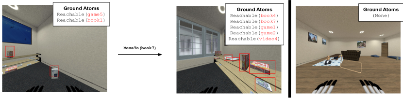
Figure 1: Example demonstration transition and evaluation task from BEHAVIOR-100 task. (Left) Visualization and high-level states for an example transition where the robot moves from being in range of picking a board game box and a book to picking 2 books, 2 board game boxes and a video game box. (Right) Visualization of an evaluation task where the robot starts out not in range of picking any objects.

A natural objective for the problem of learning a good abstract model is prediction accuracy [LOFT2021, silver2022inventing], which would be appropriate if we were using the abstract model to make precise predictions. Instead, our objective is to find an abstract model that maximally improves the performance of the bilevel planning algorithm, given the available data. The difference between these objectives is stark in many robotics domains where robot actions can affect many relationships among the robot and objects in the world. Making precise predictions about these state changes might require a very fine-grained abstract model with many complex operators. Such a model would require a lot of data to learn reliably, be very slow to plan with, and also be unlikely to generalize to novel tasks.

For example, consider the Sorting Books task from the BEHAVIOR-100 benchmark [srivastava2021behavior]. The goal is to retrieve a number of books strewn about a living room and place them on a shelf. A Reachable(?object) predicate is given to indicate when the robot is close enough to an object to pick it up. When the robot moves to pick a particular object, the set of objects that are reachable varies depending on their specific configuration. Figure 1 shows a transition where the robot moves to put itself in range of picking up book7, but happens to also be in range of picking up several other items. Optimizing prediction error on this transition would yield a very complex operator that is overfit to this specific situation and thus neither useful for efficient high-level planning nor generalizable to new tasks with different object configurations (e.g. the test situation depicted in the right panel of Figure 1, where the robot is initially not in reachable range of any objects).

⬇

Op-MoveToBook-Prediction-Error:

Args: ?objA ?objB ?objC ?objD ?objE

?objF ?objG

Preconditions: (and (Reachable ?objA)

(Reachable ?objB))

Add Effects: (and (Reachable ?objC)

(Reachable ?objD)(Reachable ?objE)

(Reachable ?objF)(Reachable ?objG))

Delete Effects: (and (Reachable ?objA)

(Reachable ?objB))

⬇

Op-MoveToBook-Necessary-Changes:

Args: ?objA

Preconditions: ()

Add Effects: (Reachable ?objA)

Delete Effects: ($\forall$?x. ?objA $\neq$ ?x $\Rightarrow$ (Reachable ?x))

In this work, we take seriously the objective of learning a set of operators that is tied to overall planning performance. We observe that, in order to generate useful high-level plans, operators need only model predicate changes that are necessary for high-level search. Optimizing this objective allows us to learn operators that generalize better and yield faster planning.

Our main contributions are (1) the formulation of a novel objective for operator learning based on planning performance, (2) a procedure for distinguishing necessary changes within the high-level states of provided demonstrations, and (3) an algorithm that leverages (1) and (2) to learn symbolic operators from demonstrations via a hill-climbing search. We test our method on a wide range of complex robotic planning problems and find that our learned operators enable bilevel planning to solve challenging tasks and generalize substantially from a small number of examples.

2 Problem Setting

We aim to develop an efficient method for solving TAMP problems in complex domains with long-horizon solutions given structured low-level continuous state and action spaces [silver2022learning, silver2022inventing, chitnis2021learning]. We assume an ‘object-oriented’ state space: a state $x\in\mathcal{X}$ is characterized by the continuous properties (e.g. pose, color, material) of a set of objects. Actions, $u\in\mathcal{U}$, are short-horizon policies with both discrete and continuous parameters, which accomplish a desired change in state (e.g., Pick(block, $\theta$) where $\theta$ is a grasp transform). These parameterized controllers can be implemented via learning or classical approaches (e.g. motion planning). We opt for the latter in all domains in this paper. Transitions are deterministic and a simulator $f:\mathcal{X}\times\mathcal{U}\to\mathcal{X}$ predicts the next state given current state and action. The state and action representations, as well as the transition function can be acquired by engineering or learning  [brady2023provably, silver2022learning, chang2017a].

PreimageBackchaining(($\Omega$,$(\overline{x},\overline{u}),\mathcal{O},g$))

      1 $n\leftarrow\text{length}(\overline{x})$ ; $\alpha_{n}\leftarrow g$

      2 for $i\leftarrow n-1,n-2,\dots,0$ do

            3 $s_{i},s_{i+1}\leftarrow\textsc{Abstract}(x_{i}),\textsc{Abstract}(x_{i+1})$

            4 $\underline{\omega}_{\text{best}}\leftarrow$ FindBestConsistentOp($\Omega$, $s_{i}$, $s_{i+1}$, $\alpha_{i+1}$, $\mathcal{O}$)

            5 if $\underline{\omega}_{\text{best}}=\text{Null}$ then

                   break

            6$\underline{\omega_{i+1}}\leftarrow\underline{\omega}_{\text{best}}$

            7 $\alpha_{i}\leftarrow\underline{P_{i+1}}\cup(\alpha_{i+1}\setminus\underline{E^{+}_{i+1}})$

            

      8return $(\underline{\omega_{i+1}},\ldots,\underline{\omega_{n}}),(\alpha_{i},\ldots,\alpha_{n})$

Algorithm 1 Preimage backchaining procedure (details in (§LABEL:appendix:data-partitioning)).

HillClimbingSearch($\mathcal{D}$)

      1 $J_{\text{last}}\leftarrow\infty$; $J_{\text{curr}}\leftarrow\textsc{J(}\Omega,\mathcal{D}{)}$

      2 $\Omega\leftarrow\emptyset$

      3 while $J_{\text{curr}}<J_{\text{last}}$ do

            4 $\Omega^{\prime}\leftarrow\textsc{ImproveCoverage(}\Omega,\mathcal{D}{)}$

            5 if $\textsc{J(}\Omega^{\prime},\mathcal{D}{)}<J_{\text{curr}}$ then

                  6 $\Omega\leftarrow\Omega^{\prime}$ ; $J_{\text{curr}}\leftarrow\textsc{J(}\Omega,\mathcal{D}{)}$

                  

            7$\Omega^{\prime}\leftarrow\textsc{ReduceComplexity(}\Omega,\mathcal{D}{)}$

            8 if $\textsc{J(}\Omega^{\prime},\mathcal{D}{)}<J_{\text{curr}}$ then

                  9 $\Omega\leftarrow\Omega^{\prime}$ ; $J_{\text{curr}}\leftarrow\textsc{J(}\Omega,\mathcal{D}{)}$

                  

            10$J_{\text{last}}\leftarrow J_{\text{curr}}$ ; $J_{\text{curr}}\leftarrow\textsc{J(}\Omega,\mathcal{D}{)}$

            

      11return $\Omega$

      

Algorithm 2 HillClimbingSearch learns operators that optimize objective $J$.

Since planning in this low-level space can be expensive and unreliable [kurutach2018learning, silver2022inventing, chitnis2021learning], we pursue a search-then-sample bilevel planning strategy in which search in an abstraction is used to guide low-level planning. We assume we are given a set of predicates $\Psi$ to define discrete properties of and relations between objects (e.g., On) via a classifier function that outputs true or false for a tuple of objects in a low-level state. Predicates induce a state abstraction $\textsc{abstract}:\mathcal{X}\to\mathcal{S}$ where $\textsc{abstract}(x)$ is the set of true ground atoms in $x$ (e.g., {HandEmpty(robot), On(b1, b2), …}). The low-level state space, action space, and simulator together with the predicates comprise an environment. To enable bilevel planning for an environment, we must learn a partial abstract transition model over the predicates in the form of symbolic operators.

We consider a standard learning-from-demonstration setting where we are given a set of training tasks with demonstrations, and must generalize to some held-out test tasks. A task $T\in\mathcal{T}$ is characterized by a set of objects $\mathcal{O}$, an initial state $x_{0}\in\mathcal{X}$, and a goal $g$. The goal is a set of ground atoms and is achieved in $x$ if $g\subseteq\textsc{abstract}(x)$. A solution to a task is a sequence of actions $\overline{u}=(u_{1},\dots,u_{n})$ that achieve the goal ($g\subseteq\textsc{abstract}(x_{n})$, and $x_{i}=f(x_{i-1},u_{i})$ for $1\leq i\leq n$) from the initial state. Each environment is associated with a task distribution. Our objective is to maximize the likelihood of solving tasks from this distribution within a planning time budget.

3 Operators for Bilevel Planning

Symbolic operators, defined in PDDL [aeronautiques1998pddl] to support efficient planning, specify a transition function over our state abstraction. Formally, an operator $\omega$ has arguments $\overline{v}$, preconditions $P$, add effects $E^{+}$, delete effects $E^{-}$, and a controller $C$. The preconditions and effects are each expressions over the arguments that describe conditions under which the operator can be executed (e.g. Reachable(?book1)) and resulting changes to the abstract state (e.g. Holding(?book1)) respectively. The controller is a policy (from the environment’s action space), parameterized by some of the discrete operator arguments, as well as continuous parameters whose values will be chosen during the sampling phase of bilevel planning. A substitution of arguments to objects induces a ground operator $\underline{\omega}=\langle\underline{P},\underline{E^{+}},\underline{E^{-}},\underline{C}\rangle$. Given a ground operator $\underline{\omega}=\langle\underline{P},\underline{E^{+}},\underline{E^{-}},\underline{C}\rangle$, if $\underline{P}\subseteq s$, then the successor abstract state $s^{\prime}$ is $(s\setminus\underline{E^{-}})\cup\underline{E^{+}}$ where $\setminus$ is set difference. We use $F(s,\underline{\omega})=s^{\prime}$ to denote this (partial) abstract transition function.

In previous work on operator learning for bilevel planning [LOFT2021, chitnis2021learning], operators are connected to the underlying environment via the following semantics: if $F(s,\underline{\omega})=s^{\prime}$, then there exists some low-level transition $(x,u,x^{\prime})$ where $\textsc{abstract}(x)=s$, $\textsc{abstract}(x^{\prime})=s^{\prime}$, and $u=\underline{C}(\theta)$ for some $\theta$. These semantics embody the “prediction error” view in that abstract must predict the entire next state ($\textsc{abstract}(x^{\prime})=s^{\prime}$). Towards implementing the alternative “necessary changes” view, we will instead only require the abstract state output by $F$ to be a subset of the atoms in the next state, that is, $\textsc{abstract}(x^{\prime})\subseteq s^{\prime}$. Thus, we permit our operators to have universally quantified single-predicate delete effects (e.g., $\forall\texttt{?v. }\texttt{Reachable(?v)}$). Intuitively, $F$ is now responsible only for predicting abstract subgoals to guide low-level planning, rather than predicting entire successor abstract states. Under these new semantics, $F$ encodes an abstract transition model where the output atoms $s^{\prime}$ represent the set of possible abstract states where these atoms hold.

Given operators, we can solve new tasks via search-then-sample bilevel planning (decribed in detail in appendix (§LABEL:appendix:bilevel-planning) and previous work [garrett2021integrated, chitnis2021learning, LOFT2021, silver2022learning, silver2022inventing]). Given the task goal $g$, initial state $x_{0}$, and corresponding abstract state $s_{0}=\textsc{abstract}(x_{0})$, bilevel planning uses AI planning techniques (e.g., helmert2006fast) to generate candidate abstract plans. An abstract plan is a sequence of ground operators $(\underline{\omega}_{1},\dots,\underline{\omega}_{n})$ where $g\subseteq s_{n}$ and $s_{i}=F(s_{i-1},\underline{\omega}_{i})$ for $1\leq i\leq n$. The corresponding abstract state sequence $(s_{1},\dots,s_{n})$ serves as a sequence of subgoals for low-level planning. The controller sequence $(\underline{C}_{1},\dots,\underline{C}_{n})$ provides a plan sketch, where all that remains is to refine the plan by “filling in” the continuous parameters. We sample continuous parameters $\theta$ for each controller starting from the first and checking if the controller achieves its corresponding subgoal $s_{i}$. If we cannot sample such parameters within a constant time budget, we backtrack and resample, and eventually even generate a new abstract plan. We adapt previous work [chitnis2021learning] to learn neural network samplers after learning operators (see (§LABEL:appendix:samplers) in the appendix for more details).

4 Learning Operators from Demonstrations

To enable efficient bilevel planning, operators must generate abstract plans corresponding to plan sketches that are likely to be refinable into low-level controller executions. Given demonstrations $\mathcal{D}$ consisting of a goal $g$, action sequence $\overline{u}$, corresponding state sequence $\overline{x}$, and set of objects $\mathcal{O}$, we wish to find the simplest set of operators such that for every training task, abstract planning with these operators is able to generate the plan sketch corresponding to the demonstration for this task.

Specifically, we minimize the following objective:

$$J(\Omega)\triangleq(1-\texttt{coverage}(\mathcal{D},\Omega))+\lambda\texttt{complexity}(\Omega)$$ (1)

where coverage is the fraction of demonstration plan sketches that planning with operator set $\Omega$ is able to produce and complexity is the number of operators. In our experiments, we set $\lambda$ to be small enough so that complexity is never decreased at the expense of coverage.

Figure 2: Environments. Visualizations for Screws, Satellites, Painting, Collecting Cans, and Sorting Books.

We will approach this optimization problem using a hill-climbing search (Algorithm 2), which benefits from having a more fine-grained interpretation of coverage defined over transitions within a trajectory instead of entire trajectories. To develop this definition, we will first introduce the notion of necessary atoms.

Definition 4.1.

Given an operator set $\Omega$, and an abstract plan $(\underline{\omega}_{1},\dots,\underline{\omega_{n}})$ in terms of $\Omega$ that achieves goal $g$, the necessary atoms at step $n$ are $\alpha_{n}\triangleq g$, and at step $0\leq i<n$ are $\alpha_{i}\triangleq\underline{P_{i+1}}\cup(\alpha_{i+1}\setminus\underline{E^{+}_{i+1}})$.

In other words, an atom is necessary if it is mentioned either in the goal, or the preconditions of a future operator in a plan. If operators in $\Omega$ model each of the necessary atoms for every timestep, then these operators must be sufficient for producing the corresponding abstract plan via symbolic planning. Moreover, each necessary atom set is minimal in that no atoms can be removed without violating either the goal or a future operator’s preconditions. Thus, we need only learn operators to model changes in these necessary atoms.

Given necessary atoms, we can now define what it means for some sequence of operators to be consistent with some part of a demonstration.