ArchEnemy: Removing scattered-light glitches from gravitational wave data.

Abstract

Data recorded by gravitational wave detectors includes many non-astrophysical transient noise bursts, the most common of which is caused by scattered-light within the detectors. These so-called “glitches” in the data impact the ability to both observe and characterize incoming gravitational wave signals. In this work we use a scattered-light glitch waveform model to identify and characterize scattered-light glitches in a representative stretch of gravitational wave data. We identify $2749$ scattered-light glitches in $5.96$ days of LIGO-Hanford data and $1306$ glitches in $5.93$ days of LIGO-Livingston data taken from the third LIGO-Virgo observing run. By subtracting identified scattered-light glitches we demonstrate an increase in the sensitive volume of a gravitational wave search for binary black hole signals by $\sim 1\%$.

1 Introduction

The Laser Interferometer Gravitational-Wave Observatory (LIGO) [1] and Virgo [2] collaborations made the first observation of gravitational waves in September 2015 [3]. The detection established the field of gravitational wave astronomy and a global network of gravitational wave detectors, now joined by KAGRA [4], has allowed for the detection of approximately 100 gravitational wave events [5, 6, 7, 8].

The detection of gravitational waves is made possible by both the sensitivity of the detectors and the search pipelines [9, 10, 11, 12, cwb_2020] which analyse raw strain data from the output of the detectors and identify observed gravitational wave signals. One of the problems that these search pipelines must deal with is the fact the data contains both non-stationary noise and short duration ‘glitches’ [13, 14, 15] where noise power increases rapidly. Glitches are caused by instrument behaviour or interactions between the instrument and the environment [16, Glanzer:2023hzf] and glitches reduce the sensitivity of the detectors [17], can potentially obscure candidate gravitational wave events [6] and can even mimic gravitational wave events [18, 19].

Different classes of glitches have been characterized using tools such as Gravity Spy [20, 21]. Of the 325,101 glitches classified by Gravity Spy in the third observing run of Advanced LIGO [22] with a confidence of $90\%$ or higher, 120,733 ($32.1\%$) were classified as “Scattered Light”. Scattered-light glitches occur in the 10-120Hz frequency band [23] which coincides with the frequency band where we observe the inspiral and merger signatures of compact binary coalescences. Scattered-light glitches are characterized by an arch-like pattern in a time-frequency spectrogram of the detector output, as seen in figure 1.

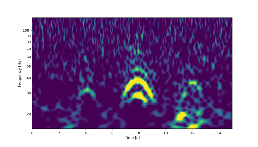
Figure 1: An Omega scan [24] of gravitational wave data containing an example of a scattered-light glitch. Scattered-light glitches are characterized by a symmetric arch-like pattern. Multiple scattered-light glitches can be seen at the 4, 8 & 12 second marks as well as multiple harmonic glitches at 8 seconds.

Scattered-light glitches occur when laser light in the interferometer is scattered from the main optical path by components within the detector. The motion of these components is coupled to seismic motion inducing a phase shift on the light being scattered as the surface moves back and forth. This scattered-light then recombines with the main laser, producing scattered-light glitches in the data. The surfaces from which scattered-light glitches originate have been objects on optical benches such as lenses, mirrors and photo-detectors [25].

Scattered-light glitches have been a significant problem when observing compact binary mergers. As an example, GW190701_203306 was coincident with a scattered-light glitch, as shown in figure 2 [6], requiring subtraction from the data before the event could be properly characterized [26]. A further 7 candidate events were found to be in coincidence with scattered-light glitches in the third observing run [8]. For this reason, it is important to reduce the effect of scattered-light glitches in the detectors and gravitational wave search pipelines. Scattered-light glitches occur as single or multiple glitches and can appear rapidly in time and simultaneously in frequency (see figure 3), which we refer to as harmonic glitches.

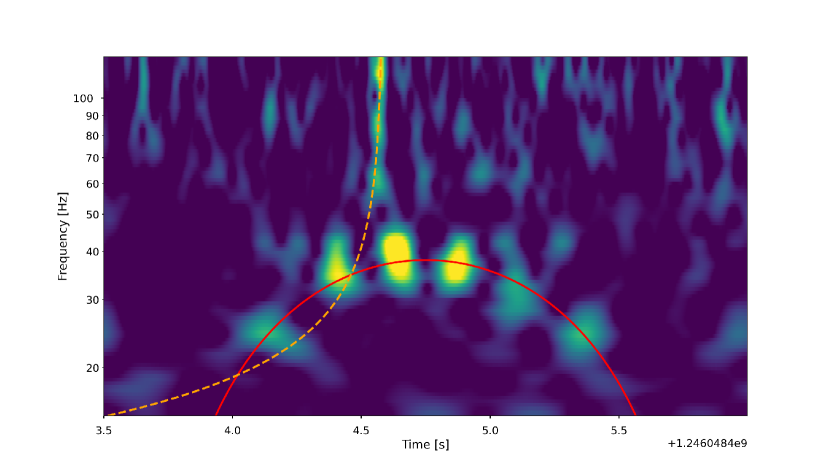
Figure 2: GW190701_203306, a gravitational wave event coincident with a scattered-light glitch in the data from the LIGO Livingston observatory. The orange dashed track shows the inferred time-frequency evolution of a gravitational wave event produced by a compact binary merger, the red solid line is an overlaid track of the approximate location of the coincident fast scattering glitches.

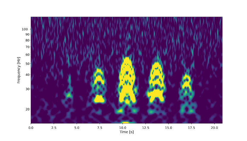
Figure 3: An Omega scan [24] of gravitational wave data containing multiple examples of scattered-light glitches. Here we see multiple scattered-light glitches repeating periodically in a $20$ second period of time. Harmonic scattered-light glitches are also seen in multiple stacks, the harmonic glitches share time period values and the glitch frequency values are $n-$multiples of the lowest frequency harmonic within the stack.

The most obvious way to remove the impact of glitches is removing the mechanisms which produce the glitches in the observatories. This has been investigated in previous works [23, 25, 27, 28, 29, 30, 31, 32], which focus on identifying the surfaces in which light is being scattered from and then mitigating the scattering by reducing the reflectivity of the surface, seismically isolating it or relocating it.

An alternative method for reducing scattered-light glitches, known as “RC tracking”, was implemented in the Advanced LIGO observatories in January 2020 [23]. The Advanced LIGO detectors employ a quadruple pendulum suspension for the test masses where two chains suspend four masses in this suspension system, one for the test mass optic and the other for the reaction mass. The reaction mass is used to impose a force upon the test mass and a significant source of scattered-light glitches was the large relative motion between the test mass chain and the reaction chain. To mitigate this effect, the relative motion between the end test mass and the reaction mass needed to be reduced. This was achieved by ensuring the two chains are moving together by applying force to the top stage of the quadruple suspension system in Advanced LIGO. The implementation of RC tracking represented a decrease from $0.01s^{-1}$ to $0.0001s^{-1}$ and $0.0072s^{-1}$ to $0.0012s^{-1}$ in the number of scattered-light glitches detected by Gravity Spy for LIGO-Hanford and LIGO-Livingston respectively.

While methods for preventing scattered-light glitches have been developed and have shown success, they have not been able to remove the problem of scattered-light glitches from the data. Additionally, as the detectors continue to be upgraded and increase in sensitivity, new sources of scattered-light glitches will continue to appear. Identifying these new sources and mitigating their effects can take many months, during which time the detectors are taking in data which might be affected by the presence of scattered-light glitches. Therefore, it is not realistic to believe that analyses will be able to regularly run on data that does not contain scattered-light glitches and this motivates us to develop a technique for mitigating the impact of these glitches when trying to identify compact binary mergers in gravitational wave data.

In this work we present a new method for identifying and removing scattered-light glitches from gravitational wave data in advance of running searches to identify compact binary mergers. We first introduce a method for identifying when scattered-light glitches are present in detector data, through the creation of a new modelled search for scattered-light glitches, similar to how we search for gravitational waves using matched filtering. We can model scattered-light glitches, generate a suitable set of glitch waveforms and perform a matched filter search on detector data. We then subtract identified glitches from the data to increase detector sensitivity. The detector data isn’t Gaussian and stationary so the matched filter does have the potential to identify non-scattered-light glitches, and potentially even gravitational wave signals, as scattered-light glitches. To prevent this we also demonstrate a new scattered-light $\chi^{2}$ test, which can distinguish between scattered-light glitches, and other glitches—and gravitational wave signals—in the data.

We begin by reviewing previous research and describing the formulation of the waveform model used for characterizing scattered-light glitches in section 2. In section 3 we introduce the various techniques used in the search to identify scattered-light glitches in gravitational wave data and the results of the scattered-light glitch search. In section 4 we describe the results of a “glitch-subtracted” gravitational wave search and any increases in sensitivity. We conclude in section 5 and discuss the implementation of this method in future observing runs.

2 Scattered-light

To identify scattered-light glitches in gravitational wave data requires an accurate model of scattered-light glitches. This section details the derivation of the model we will use for generating our scattered-light glitch filter waveforms, along with its parameterization.

2.1 Modelling scattered-light glitches - a review

Our model for scattered-light glitches draws heavily from [25], and we briefly review the main details of the model presented there. In [25], the authors construct a model to accurately predict the increase in noise due to scattered-light during periods of increased micro-seismic activity. The model in [25] is constructed from parameters related to physically measurable properties of the detector such as the mirror transmission factor, $T$, the finesse of the Fabry–Pérot cavity, $F$, or the wavelength of the light, $\lambda$.

They define the amplitude of the additional beam produced by light scattering off of a surface as

$$A_{sc}=A_{0}T\sqrt{\frac{2F}{\pi}}\sqrt{f_{sc}}e^{i\phi_{sc}}\,,$$ (1)

where $A_{0}$ is the amplitude of the light resonating in a Fabry–Pérot cavity, $f_{sc}$ is the fraction of the optical power scattered back into the main beam and $\phi_{sc}$ is the phase angle modulated by the displacement of the scattering optics, defined as

$$\phi_{sc}(t)=\frac{4\pi}{\lambda}(x_{0}+\delta x_{opt}(t)),$$ (2)

where $\delta x_{opt}$ is the displacement of the scattering surface and $x_{0}$ is the static optical path.

The total amplitude of the beam inside the arm is given by $A_{tot}=A_{0}+A_{sc}$, with a phase angle equal to the phase noise introduced by the scattered-light $\delta\Phi=\frac{A_{sc}}{A_{0}}\cdot\sin\phi_{sc}$. The noise introduced by the scattered-light, $h_{sc}$, can be approximated through the relationship $\sin(\Phi_{0}+\delta\Phi)\approx\cos(\Phi_{0})\times\sin(\delta\Phi)$ for small $\delta\Phi$, and can be expressed as

$$h_{sc}(t)=G\cdot\sin\left(\frac{4\pi}{\lambda}(x_{0}+\delta x_{sc}(t))\right),$$ (3)

where $G$ is the coupling factor, defined as $K\cdot\sqrt{f_{sc}}$ where

$$K=\frac{\lambda}{4\pi}\frac{T}{\sqrt{2F\pi}}.$$ (4)

The displacement of the scatterer when presenting with oscillatory motion is then given as

$$\delta x_{sc}(t)\simeq A_{m}\sin(2\pi f_{m}t),$$ (5)

where $f_{m}$ is the frequency-modulated signal with modulation index $m=A_{m}\frac{4\pi}{\lambda}$ and where $A_{m}$ is the amplitude of the $n$th harmonic. Finally, equation 3 can be simplified when considering only small bench motion, according to

$$h_{sc}(t)=G\cdot\cos\phi_{0}\cdot\frac{4\pi}{\lambda}\cdot\delta x_{sc}(t)\;.$$ (6)

2.2 Model

The model introduced in [25] for the gravitational wave strain noise introduced by scattered-light uses a lot of knowledge about the detector state. The model used in this work will be more phenomenological in the parameterization, allowing us to rely only on the characteristics of the glitches in the strain data and not knowledge of the detector configuration, especially in cases where this detector information might not be known. Each scattered-light glitch, as viewed in a spectrogram (see figure 1), has two easily identifiable features: the maximum frequency reached, glitch frequency ($f_{gl}$); and the period of time the glitch exists in detector data, time period ($T$). In addition we can fully describe an artifact by defining an amplitude ($A$), phase ($\psi$) and center time of the glitch ($t_{0}$).

To formulate a model of scattered-light glitches in terms of these parameters, we simplify equation 6, treating the strain noise caused by scattered-light as the sinusoidal function

$$h_{sc}(t)\propto\sin(\phi_{noise}(t)).$$ (7)

Here the induced phase noise ($\phi_{noise}$) is equal to

$$\phi_{noise}(t)=2\pi f_{rep}t,$$ (8)

and $f_{rep}$ is the frequency of repetition of the sinusoid and is directly related to the time period, $T$,

$$f_{rep}=\frac{1}{2T}.$$ (9)

The time period of a scattered-light glitch only corresponds to half of a sinusoidal wave hence the multiplier of 2 on the denominator of equation 9.

Scattered-light glitches are caused by the physical increase in the distance travelled by the light as a consequence of being reflected off of a surface. The light returning to the beamsplitter from one arm will have travelled a different path length compared to the other arm and this path difference will act as a phase difference between the two arms causing non-destructive interference. The path difference and phase difference can be related with

$$\Delta\phi_{scattering}(t)=2\cdot\frac{2\pi}{\lambda}\Delta x(t),$$ (10)

where $\Delta x(t)$ indicates the change in the path taken by the light over time. An additional multiplier of 2 indicates our path difference is occurring twice, once when the light approaches the surface and again when leaving.

We assume the scattering surfaces are oscillatory in motion and apply the same simplification made in equation 5, with an initial position $\Delta x=0$ to a maximum displacement of $x_{0}$. This produces an equation for the path difference of the light,

$$\Delta x(t)=x_{0}\sin(2\pi f_{rep}t).$$ (11)

We substitute equation 11 into equation 10 and produce an equation for the phase noise induced by scattered-light

$$\phi_{scattering}(t)=\frac{4\pi}{\lambda}x_{0}\sin(2\pi f_{rep}t)\;,$$ (12)

this equation for the phase noise induced by scattered-light, $\phi_{scattering}(t)$, and the equations for the generic phase noise, $\phi_{noise}(t)$ (equation 8), can now be used to create an equation for the strain noise caused by scattered-light.

We take the derivatives of equations 8 $\&$ 12 with respect to time:

$$\phi_{noise}^{\prime}(t)=2\pi F_{inst}(t),$$ (13)

$$\phi_{scattering}^{\prime}(t)=\frac{4\pi}{\lambda}x_{0}2\pi f_{rep}\cos(2\pi f_{rep}t)\;,$$ (14)

where $F_{inst}$ is the instantaneous frequency at a specific time. We generate scattered-light glitches from $\frac{-T}{2}$ to $\frac{T}{2}$ to ensure their maximum frequency occurs at $t=0$. We define this maximum frequency as the glitch frequency.

We equate the two derivatives and set $t=0$, this replaces $F_{inst}(t)$ with $f_{gl}$ and $\cos(2\pi f_{rep}t)$ with $1$, then re-arrange to find the maximum displacement of the scattering surface, $x_{0}$, as

$$x_{0}=\frac{f_{gl}}{f_{rep}}\frac{\lambda}{4\pi}.$$ (15)

Substituting equation 15 into equation 12 gives us an expression for the scattered-light phase noise,

$$\phi_{scattering}(t)=\frac{f_{gl}}{f_{rep}}\sin(2\pi f_{rep}t),$$ (16)

and substituting equation 16 as our $\phi_{noise}$ in equation 7 we arrive at our model of scattered-light glitches,

$$h_{sc}(t)=A\sin\left(\frac{f_{gl}}{f_{rep}}\sin(2\pi f_{rep}t)+\psi\right),$$ (17)

where $A$ and $\psi$ are amplitude and phase parameters to be maximised over.

In [32] they provide another term to describe scattered-light glitches which uses the instantaneous frequency as a function of time, allowing the identification of the correct amplitude at all frequencies. This term is due to radiation pressure coupling and is thought to be dominant at low frequencies. The relationship between our amplitude and the new amplitude depends on the power in the arm cavities and the signal recycling mirror reflectivity which we do not consider in our model and so disregard this extra term.

2.3 Harmonics

As described in [25], harmonic glitches appear at the same time with different glitch frequencies. A harmonic glitch is a glitch with a glitch frequency that is a positive integer multiple of the glitch frequency of the glitch in the stack with the lowest glitch frequency value. This lowest frequency glitch has the potential to appear below $15$Hz and will be masked by other sources of noise and therefore cannot be seen. An example of harmonics can be seen in figure 3.

3 Identifying scattered-light glitches in gravitational wave strain data

Equipped with our model for scattered-light glitches from the previous section, we now discuss how we identify and parameterize scattered-light glitches in a stretch of gravitational wave data before we apply this to searches for compact binary mergers in the next section.

3.1 Matched Filtering

Given our model of scattered-light glitches, we can consider a realization with specific values of the parameters discussed above. To identify glitches with these values of the parameterization, we follow the same technique as that commonly used to identify compact binary mergers and apply matched filtering. The matched filter is defined as [33].

$$\rho(t)=\frac{(h|s)}{\sqrt{(h|h)}}\equiv(\hat{h}|s).$$ (18)

Here $h$ is the model template, $s$ the gravitational wave data we are searching and we use the noise-weighted inner product defined between two time series $a(t)$ and $b(t)$ as

$$(a|b)=4Re\int^{\infty}_{0}\frac{\tilde{a}(f)\tilde{b}^{*}(f)}{S_{n}(f)}df.$$ (19)

The tilde on $\tilde{a}$ and $\tilde{b}$ refer to the Fourier-transform of both variables into the frequency domain. The denominator, $S_{n}(f)$, represents the one-sided power spectral density (PSD) of the data, defined as

$$\langle\tilde{s}(f)\tilde{s}(f^{\prime})\rangle=\frac{1}{2}S_{n}(f)\delta(f-f^{\prime})\;,$$ (20)

where the angle brackets denote an average over noise realizations and $\delta$ is the Dirac delta function.

Scattered-light glitches will take a range of values of the parameters describing them and we must be able to identify glitches anywhere in the parameter space. Following [33] we can analytically maximize over the amplitude, phase and the center time glitch parameters in equation 17. The matched filter naturally maximizes over amplitude when expressed in terms of signal-to-noise ratio, and can be evaluated as a function of time by including a time shift in equation 19,

$$(a|b)(t)=\left|4Re\int^{\infty}_{0}\frac{\tilde{a}(f)\tilde{b}^{*}(f)}{S_{n}(f)}e^{-2\pi ift}df\right|.$$ (21)

To maximize over phase we take the absolute value of the inner product, rather than the real part of the integral.

3.2 Template Bank

Our scattered-light glitch model is parameterized by 5 variables. As shown above, by maximizing over phase, amplitude and time, we can analytically maximize the signal-to-noise ratio over 3 of these variables. However, the remaining two describe the intrinsic evolution of the glitch and we must explicitly search over these parameters. To do this we create and use a “template bank” of scattered-light glitch waveforms, created such that it would be able to identify glitches with any value of our 2 remaining parameters, glitch frequency and time period.

To generate this template bank, a stochastic template placement algorithm [34] is used. This algorithm randomly generates a new template, places the template in the existing template bank and calculates the “distance” (how similar two templates appear) between the new template and existing templates. If the new template is too close to an existing template it is discarded, otherwise, it is accepted into the bank. The density of the bank is dependent on the allowed distance between two templates. The dominant cost of the search for scattered-light glitches is matched filtering and is approximately linear in the number of templates, a larger template bank will find all of the glitches with more accurate parameter values but the computational cost of the search will be increased. The template bank generation alone does not constitute a significant computational cost in the search.

The distance function we have chosen to evaluate templates by is the match between two glitch templates. To calculate the match, we first normalize both templates such that the matched filter between a template and itself would be equal to 1. We can then compute the inner product between the two normalized templates to find their match

$$M=\max_{t,\psi}(\hat{a}|\hat{b}).$$ (22)

The value for the match, $M$, is bounded between 0 and 1, where a value of 0 indicates orthogonal waveforms and a value of 1 indicates identical normalized waveforms. The maximum match allowed between any two templates in our bank is 0.97, which implies that a fully converged stochastic bank would have at least one waveform in it with $M\geq 0.97$ for any point in the space of parameters.

For our scattered-light glitch search, we generated a template bank with time periods $\in$ $1.8$s - $5.5$s and glitch frequencies $\in$ $20$Hz - $80$Hz. We chose to use the Advanced LIGO zero-detuned high-power sensitivity curve [35]. This allowed us to generate a template bank that contains 117,481 templates. We visualize the distribution of the templates as a function of time period and glitch frequency in figure 4, observing a greater density of templates at higher frequencies and longer durations.

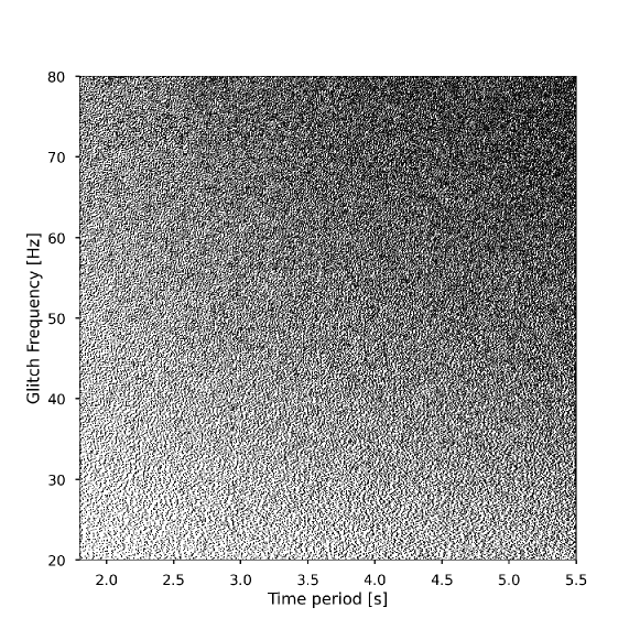
Figure 4: The template bank of scattered-light glitch templates (black points) used in the search for scattered-light glitches. The glitch frequency parameter values range from $20$Hz - $80$Hz and the time period parameter values range from $1.8$s - $5.5$s. This bank was created with a maximum match allowed between two templates of $0.97$ and contains 117,481 templates.

3.3 Identifying potential scattered-light glitches in the data

We test our method by searching through gravitational wave data from 2019-11-18 16:13:05 - 2019-11-25 22:11:09 for the LIGO-Hanford and LIGO-Livingston detectors. This time corresponds to the 25th period of data used in the LVK analysis of O3 data for compact binary mergers [8] and is prior to the implementation of RC tracking [23] in these detectors. We only analyse data that is flagged as “suitable for analysis” on the Gravitational Wave Open Science Center [36]. This corresponds to 5.96 days of analysable data for LIGO-Hanford and 5.93 days for LIGO-Livingston.

Equipped with our template bank we now identify potential scattered-light glitches in the data. We matched filter all of the data against all of the templates, producing a signal-to-noise ratio time series for every template in the bank. These signal-to-noise ratio time series will contain peaks which, when above a certain limit, indicate the presence of a scattered-light glitch at a particular time. We retain any maxima within the time series that have a signal-to-noise ratio greater than 8. However, as we do this independently for every template, we will identify multiple peaks for any given glitch, and we will also find peaks that correspond to other types of glitch, or even gravitational wave signals. We discuss how we reduce this to a list of identified scattered-light glitches in the following subsections.

3.4 Scattered-Light Signal Consistency Test

To prevent the search for scattered-light glitches from misclassifying other classes of glitches, or gravitational wave signals, we employ a $\chi^{2}$ consistency test. The $\chi^{2}$ discriminator introduced in [37] divides gravitational wave templates into a number of independent frequency bins. These bins are constructed so as to contain an equal amount of the total signal-to-noise ratio (SNR) of the original matched filter between template and data. The $\chi^{2}$ value is obtained by calculating the SNR of each bin, subtracting this from the expected SNR value for each bin and squaring the output. These values are summed for all bins and this value forms the $\chi^{2}$ statistic,

$$\chi_{r}^{2}=\frac{\chi^{2}}{\textrm{DOF}}=\frac{n}{2n-2}\sum_{i=1}^{n}\left(\frac{\rho}{\sqrt{n}}-\rho_{bin,i}\right)^{2}.$$ (23)

Here $n$ is the number of bins, $\rho$ is the SNR of the original matched filter between template and data, and $\rho_{bin}$ is the value of the SNR found when matched filtering one of the divided templates and the data. This test is constructed so as to produce large values when the data contains a glitch, or astrophysical signal, that is not well described by the template, but to follow a $\chi^{2}$ distribution if a glitch that matches well to the template is present, or if the data is Gaussian and stationary.

The $\chi^{2}$ test that we employ is similar to that of [37], however compact binary merger waveforms increase in frequency over time whereas scattered-light glitch templates are symmetric about their centre. We therefore choose to construct our $\chi^{2}$ test with four non-overlapping bins in the time domain, each of which contributes equally to the SNR, an example of the split template can be seen in figure 5. The matched filter between the bins and data is computed and the $\chi_{r}^{2}$ value is calculated using equation 23 (where $n=4$). Any glitch, or astrophysical signal, which does not exhibit symmetric morphology should not fit with this deconstruction of the template, and should result in elevated $\chi_{r}^{2}$ values.

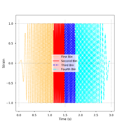
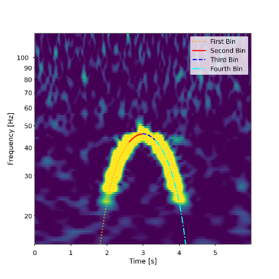
Figure 5: A scattered-light glitch template (left) where the colours and line-styles are indicative of the four equal SNR time bins to be used in calculating the $\chi_{r}^{2}$ value and re-weighting the SNR. The same scattered-light glitch template bins overlaid on an injection of the scattered-light glitch (right). The inner two bins are considerably shorter than the outer two bins which informs us that the center - higher frequency - region of the scattered-light glitch contributes a larger amount to the SNR per unit time than the lower frequency regions.

After computing the $\chi_{r}^{2}$ value for potential scattered-light glitches, we follow [38] to compute a “re-weighted signal-to-noise ratio”, which is an empirically tuned statistic depending on the signal-to-noise ratio and the $\chi_{r}^{2}$ value. The re-weighting function we use matches that presented in [38],

$$\rho_{rw}=\left\{\begin{array}[]{l@{\quad}cr}\rho&\mathrm{if}&\chi_{r}^{2}\leq 1,\\ \rho[(1+(\chi_{r}^{2})^{3})/2]^{-\frac{1}{6}}&\mathrm{if}&\chi_{r}^{2}\geq 1,\end{array}\right.$$ (24)

where $\rho_{rw}$ represents the re-weighted signal-to-noise ratio of the scattered-light glitch template calculated using the signal-to-noise ratio, $\rho$, and the $\chi_{r}^{2}$ value of that template. We do note that this re-weighting function has been tuned for compact binary merger waveforms and we did not repeat that tuning here with scattered-light glitches. One could retune this statistic, specifically targeting scattered-light glitches, using (for example) the automatic tuning procedure described in [39]. However, we demonstrate the suitability of the $\chi^{2}$ test for our purposes in figure 6 where we show the $\chi_{r}^{2}$ vs SNR distribution of the triggers found by our scattered-light glitch search when performed on data containing only scattered-light glitches and data containing a binary black hole gravitational wave injection.

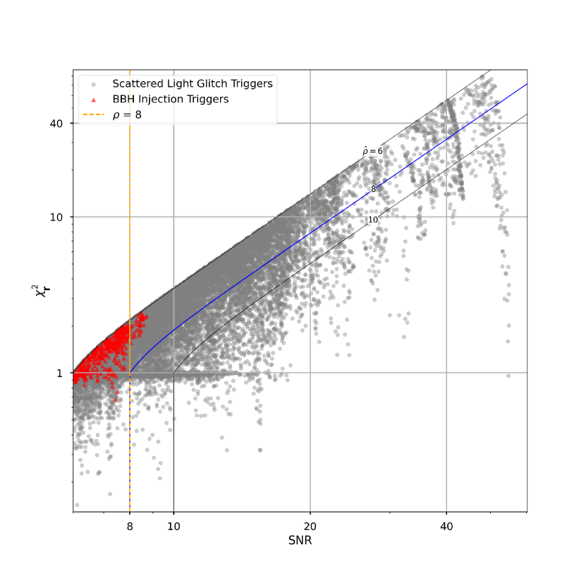
Figure 6: The signal-to-noise ratio and $\chi_{r}^{2}$ values for the triggers identified by the matched filtering and clustering of the scattered-light glitch template bank with data containing only scattered-light glitches (grey hexagons) and data containing a binary black hole gravitational wave injection (red triangles). The black contour lines represent the re-weighted signal-to-noise ratio values the trigger will take when equation 24 is applied. The orange dashed vertical line indicates the signal-to-noise ratio value limit of 8, above which we decide to perform the $\chi^{2}$ test and calculate the re-weighted signal-to-noise ratio. The blue solid contour line indicates a re-weighted signal-to-noise ratio value of 8, which is the limit at which we consider the trigger to be real. Different re-weighting parameter values will produce different contour line shapes. It can be seen that no triggers for the data containing the gravitational wave injection lie beneath the contour line and therefore no scattered-light glitches are found on the gravitational wave signal.

We note that the $\chi^{2}$ test increases the number of matched filters required by the search and therefore the computational cost of the search. Each template would require the matched filtering of an additional $4$ “binned” templates to calculate the $\chi_{r}^{2}$ value to re-weight the SNR time series of that template, increasing computational cost by a maximum factor of $5$. However, we reduce this increase by only computing the $\chi^{2}$ where it is needed, specifically for any template where the SNR time series has values above the threshold of 8.

3.5 Identifying all scattered-light glitches in the data

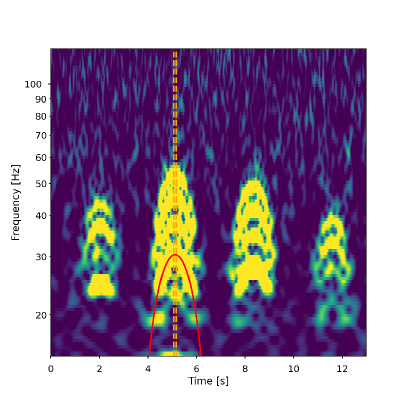
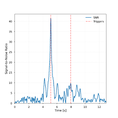
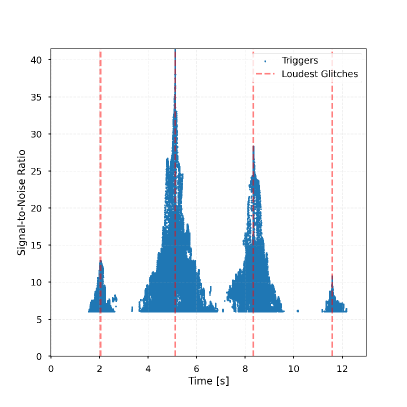
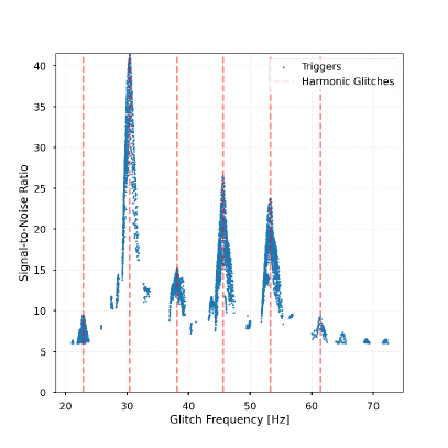
Figure 7: The process for identifying all the scattered-light glitches in a period of gravitational wave data. The red overlay in the gravitational wave data used in this example (top left) indicates the highest re-weighted signal-to-noise trigger found, the dashed vertical lines represent the time slice window around this trigger. The re-weighted signal-to-noise ratio time series resulting from the matched filter of this trigger’s template and the data (top right) is clustered in time to identify the triggers found above a signal-to-noise threshold of $8$, indicated by red vertical dashed lines. All the triggers from all of the templates in the template bank are then clustered in time (bottom left) to identify the highest re-weighted signal-to-noise glitches in the data, indicated by the orange vertical dashes lines. The triggers found within the time slice window, with a similar time period value—within $\pm 10\%$—of the highest re-weighted signal-to-noise ratio trigger (bottom right) are clustered by their glitch frequency value to find the harmonic glitches at the same time, indicated again by red dashed lines.

Our matched filtering process retains “triggers” (potential scattered-light glitches) wherever the re-weighted signal-to-noise time series is larger than 8. We retain no more than one trigger within a window size equal to half the time period of the template used to produce the re-weighted signal-to-noise time series and only store triggers at local maxima. A re-weighted signal-to-noise time series with multiple peaks and identified triggers can be seen in the top right panel in figure 7.

After matched filtering all the templates against the data we will recover multiple triggers for any potential scattered-light glitch, as we might expect to independently identify peaks in multiple templates around the true values of the glitch. We therefore collect all of the triggers generated by the template bank and cluster these in time, using a window of half of the shortest duration template - $0.9$ seconds. This will result in a list of triggers corresponding to the highest re-weighted signal-to-noise ratios, where each trigger should correspond to a unique scattered-light glitch. The bottom left panel in figure 7 shows an example of the triggers found by the search and the highest re-weighted signal-to-noise ratio triggers found by clustering.

However, we also expect to see instances of harmonic glitches which are produced by the same scattering surface and so share the same time period and have glitch frequency values equal to a multiple of the lowest frequency glitch in the harmonic stack [25]. We investigate each trigger in the list, searching for harmonic glitches occurring at the same time. We use the first list of triggers identified by all templates across the bank and filter by those that occur within $\pm 0.05$ seconds of the center time of the trigger we are investigating, an example of this window can be seen in the top left panel of figure 7. We then filter the triggers again, keeping only those with an associated time period value within $\pm 10\%$ of the trigger’s time period. Finally we cluster these remaining triggers by their associated glitch frequency using a window size of $4$Hz, a lower limit on the frequency separation of harmonic glitches, the bottom right panel in figure 7 shows the identification of harmonic glitches for the overlaid scattered-light glitch in the top left panel of figure 7.

3.6 Hierarchical subtraction to find parameter values

We now have a list of identified scattered-light glitches and their parameter values, however, these might not be fully accurate when there are many glitches close in time and frequency, as illustrated in figure 8. It is important that the parameters we find match well with the glitches in the data to remove as much power as possible.

To better identify the parameter values of the scattered-light glitches, we perform a hierarchical procedure using information about the glitches we have found so far. Firstly, we create new segments of time which we know contain scattered-light glitches, taking a window of $8$ seconds on either side of each previously identified glitch, if two glitch windows overlap they are combined into the same segment.

For each segment we then create a reduced template bank, consisting of templates “close” to the scattered-light glitches previously identified in the segment. We take the smallest and largest time period and glitch frequency glitches in the segment and bound the retained templates by these values with $\pm 0.25$ seconds on the time period and $\pm 1$Hz on the glitch frequency. For each data segment the reduced template bank is matched filtered with the data, the maximum re-weighted SNR value is found and the corresponding glitch is subtracted. We then matched filter again and remove the next largest re-weighted SNR template. This process is repeated until no templates, when matched filtered with the data, produce any re-weighted SNR values above the SNR limit of $8$. This method of hierarchical subtraction produces our final list of scattered-light glitches.

A further benefit of using these shorter data segments is that we are estimating the PSD of the data using only a short period of data close to the scattered-light glitches being removed. This protects us from a rapidly changing PSD in non-stationary data, which might cause Gaussian noise to be identified with larger SNR in the periods where the PSD is larger. This can be resolved by including the variation in the power spectral density as an additional statistic in the re-ranking of triggers, which has been done for compact binary coalescence gravitational wave searches in [40].

We demonstrate the hierarchical subtraction step on an amount of data which contains four injected scattered-light glitches in a single harmonic stack, this can be seen in figure 9. As shown, the scattered-light glitches are found and subtracted from the data leaving behind a cleaned segment of gravitational wave data with no excess noise. Figure 8 shows the identified scattered-light glitch triggers before and after performing the hierarchical subtraction step on a stretch of data containing real scattered-light glitches. We identify more triggers prior to performing hierarchical subtraction, however there are more errant mismatches between scattered-light glitches and the overlaid templates. By performing the hierarchical subtraction, we more accurately identify scattered-light glitches, however, we miss some glitches that were previously identified. There is still some imperfection in this process and we do not refine the method further in this work, but highlight this as useful direction for future studies in removing scattered-light glitches.

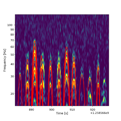
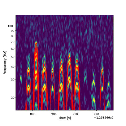
Figure 8: LIGO-Hanford data from 2019-11-23 17:54:22 - 2019-11-23 17:55:12 containing scattered-light glitches which have been identified by the ArchEnemy search (left), there is a misalignment in the template found for a number of glitches in this period of data and some missed glitches. Scattered-light glitches remaining after running the hierarchical subtraction search (right) for the same period of data, we have missed more scattered-light glitches however misalignments have been removed. The highest harmonic at approximately $892$ seconds has been incorrectly split into two separate templates.

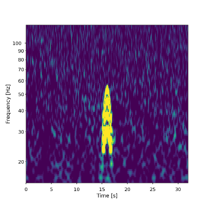
Figure 9: Data containing an injected stack of harmonic scattered-light glitches (left) and the corresponding data found when running the hierarchical subtraction search and subtracting the identified scattered-light glitches from the data (right).

3.7 Identified scattered-light glitches

The methodology described in previous sections is implemented in our “ArchEnemy” pipeline, which is capable of searching for scattered-light glitches in gravitational wave data using a pre-generated bank of glitch templates. We use ArchEnemy to analyse the aforementioned data, which produced a list of $2749$ scattered-light glitches in data from the LIGO-Hanford observatory and $1306$ from the LIGO-Livingston observatory.

The number of scattered-light glitches found by the ArchEnemy pipeline can be compared to Gravity Spy for the same period of time. Gravity Spy finds $2731$ and $1396$ for LIGO-Hanford and LIGO-Livingston respectively [20]. There will be a difference in the number of glitches found by ArchEnemy and Gravity Spy for at least two reasons: Gravity Spy treats an entire stack of harmonic glitches as a single scattered-light glitch whereas ArchEnemy will identify each glitch as a separate occurrence. Gravity Spy can also identify scattered-light glitches which are not symmetric and fall outside our template bank, for example, the scattered-light glitches shown in figure 10.

Figure 8 is an example of the results of the ArchEnemy pipeline and how well it has identified scattered-light glitches in a period of data. A majority of the glitches have been identified with the correct parameter values and even in cases where the chosen template is not visually perfect, there is a good match between the template and the identified power in the data, particularly in the case of slightly asymmetric glitches. Figure 10 demonstrates a period of time where the ArchEnemy pipeline has not fitted well the scattered-light glitches in the data. The glitches at this time are improperly fit by the templates due to asymmetry of the morphology of the glitches and because some of the glitches are outside of our template bank parameter range. However, we note that this is a very extreme period of scattered-light glitching and immediately after this time the detector data is no longer flagged as “suitable for analysis”.

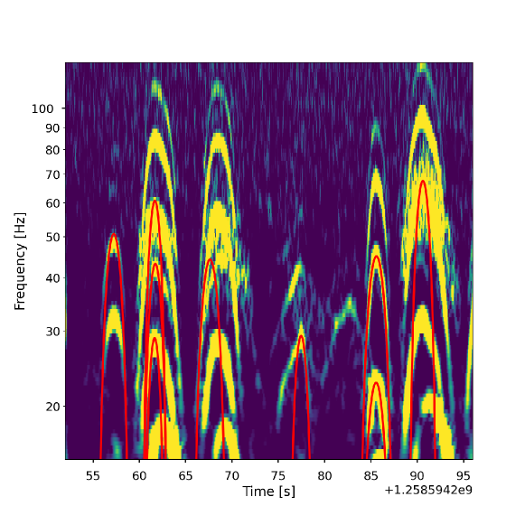
Figure 10: LIGO-Livingston data from 2019-11-24 01:30:32 - 2019-11-24 01:31:20 containing a very large number of scattered-light glitches at multiple times and frequencies over-plotted with the scattered-light glitches identified by the ArchEnemy search. Very few overlays match well onto scattered-light glitches. The template bank used in this search terminates at $80$ Hz and so the scattered-light glitches located above this value will not be correctly identified. There are also asymmetric scattered-light glitches located which will not be identified correctly by our search which assumes symmetry in the scattered-light glitch.

We have demonstrated the ArchEnemy pipeline on a stretch of data from O3 and have identified and characterized a list of scattered-light glitches, which could be removed from the data. We do note that there are cases where the identification has not worked well, but we expect that subtracting our list of glitches from the data will reduce their effect on the gravitational wave search. In the next section we will demonstrate this by quantifying sensitivity with the PyCBC pipeline.

3.8 Safety of scattered-light identification

The data we have searched through contains no previously identified gravitational wave signals [8]. However, there is a risk that the ArchEnemy search would identify real gravitational wave signals as scattered-light glitches. To assess this possibility we simulate and add a large number of gravitational wave signals into the data and assess whether any signals are misidentified.

To do this, we use three separate sets of simulated gravitational wave signals (or “injection sets”), one for BBHs, another for binary neutron stars (BNSs) and a third for neutron star black hole (NSBH) systems. We use the same simulations as the LVK search of this data, detailed in the appendix of [8]. Each injection set consists of $6200$ simulated signals spaced between $82$ and $120$ seconds apart. We treat these injection sets exactly the same as for the injection-less data, adding the simulations to the data, and then running ArchEnemy to produce a list of scattered-light glitches for each injection set.

To determine whether we have misidentified any gravitational wave injections as scattered-light glitches we look for glitches we have found within the overlapping frequency band of gravitational wave signals and our scattered-light glitch template bank. This corresponds to approximately $15$ second before merger time for the injections. The simulated signals occur every $\sim 100$ seconds so we expect to see glitches within this $15$ second window, therefore, we also require that there must be more triggers identified in the scattered-light glitch search with injections when compared to the search without injections within the window. The details of the number of gravitational wave injections with overlapping scattered-light triggers can be seen in table 1.

Table 1: For both interferometers and all $3$ injection sets we identify the number of injections which are found to have scattered-light glitches identified within $15$ seconds of merger time (“Injections with Coincident Triggers”), along with the number of scattered-light glitches found within this window for these injections (“Scattered-Light Coincident Triggers”). We investigated each of these injections and recorded the number which actually had scattered-light glitches identified due to the injected gravitational wave signal (“Actual Overlapped Injections”).

		Injections with	Scattered-Light	Actual Overlapped
Interferometer	Injection Set	Coincident Triggers	Coincident Triggers	Injections
H1	BBH	20	45	1
	BNS	23	50	2
	NSBH	38	73	7
L1	BBH	13	21	2
	BNS	18	30	2
	NSBH	35	56	16

A scattered-light glitch will be identified close to a gravitational wave signal in two cases: the ArchEnemy search is misidentifying the gravitational wave signal as a glitch or the simulated signal was added close to actual glitches and a change in the data has meant a different number of glitches has been identified. The presence of real scattered-light glitches means we might miss a gravitational wave signal, therefore, we do want to find and subtract glitches close to gravitational wave signals, but we do not want to subtract power from the gravitational wave signal itself. The scattered-light glitch $\chi^{2}$ test was designed to prevent the matching of scattered-light glitch templates on other causes of excess power, however, these results show it is not perfect.

We investigate each injection with coincident scattered-light triggers, seeing how many had misidentified scattered-light glitches on the inspiral of the gravitational wave signal, this number can be seen in the column “Actual Overlapped Injections” in table 1. We have included an example of the matching of scattered-light glitches onto gravitational wave injections in figure 11, the right panel shows the gravitational wave data post glitch subtraction where it can be seen there is a portion of the power being subtracted from the signal. Although power is being removed from the signal, the gravitational wave injection is still found by the search for gravitational waves, which we will describe later. For the cases that we have investigated, we note that the behaviour shown in figure 11 only happens for signals that have very large signal-to-noise ratio, and are therefore unphysically close to us. A similar effect is observed with the “autogating” process, described in [9], which prevents the detection of these loud signals. In contrast to the “autogating” though, signals like that illustrated in figure 11 are still identified as gravitational wave signals by the PyCBC search after scattered-light glitch removal.

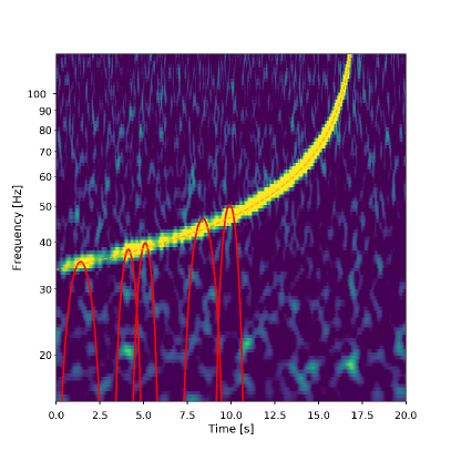
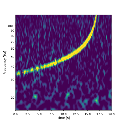
Figure 11: An injected binary neutron star compact binary coalescence gravitational wave signal, with the scattered-light glitches identified by the ArchEnemy search pipeline overlayed in red (left). The same injected signal but with the scattered-light glitches removed from the data (right). It can be seen that power is removed from the signal track and also there is an amount of power added to the data above the track.

4 Assessing sensitivity gain from removing scattered-light glitches

We now assess whether removing our identified list of scattered-light glitches results in a sensitivity gain when searching for compact binary mergers. We do this by comparing the results from the offline PyCBC search on the original data, to the results of the same search but analysing data where the glitches have been removed.

4.1 Comparing search results with and without glitch subtraction

The PyCBC pipeline is able to assess significance of potential compact binary mergers in a given stretch of data, and does the same with a set of simulated signals. This significance is quoted in terms of a “false-alarm rate”, which denotes how often we would expect to see a non-astrophysical event at least as significant as the coincident trigger being considered. In this work we assess sensitivity at a false-alarm threshold of 2 background events every year.

The data we have searched over contained no previously found gravitational wave signals [8] and our search after subtracting scattered-light glitches identified no new gravitational wave signals. While the search hasn’t found any gravitational waves, we can still measure the improvement in the sensitivity of the detectors by comparing the number of simulated signals identified with a false-alarm rate below 2 per year for each injection set (described in section 3.8) with and without removing glitches from the data. Table 2 shows the number of injections found for all injection sets and both searches.

Table 2: The number of injections found by each search with a false-alarm rate less than 2 per year alongside the number of newly-found and newly-missed injections, those found by the glitch-subtracted and not the original search and vice versa. We also show the sensitivity ratio of the glitch-subtracted search and original search for each injection set.

Injection	Original	Glitch-	Sensitivity	Newly	Newly
Type	Search	Subtracted	ratio	Found	Missed
BBH	1215	1222	1.01	10	3
BNS	1315	1315	1.00	5	5
NSBH	1260	1265	1.00	8	3

We compare the number of injections found by both searches but also look at the gravitational wave injections found by the original search and missed by the glitch-subtracted search and vice versa, this information can be seen in table 2. Considering signals found by the original search and missed by the glitch-subtracted search there are $3$ binary black hole injections with false-alarm rates in the original search ranging from $0.5-0.3$ per year, one of which had a glitch removed approximately $9$ seconds after the injection, there are $5$ newly-missed binary neutron star injections with false-alarm rates ranging from $0.5-0.056$ per year, two of the five binary neutron star injections had glitches removed within $60$ seconds of the injection, and there are $3$ newly-missed neutron star black hole injections with false-alarm rates ranging from $0.5-0.086$, one had glitches removed within $60$ seconds of the injection. The other newly-missed injections showed no scattered-light glitches within a $20$ second window for binary black hole injections and a $60$ second window for binary neutron star and neutron star black hole injections.

The glitch-subtracted search identifies $10$ additional binary black hole injections, the most significant of which have false-alarm rates of 1 per $190.50$, 1 per $7633.84$ and 1 per $8643.73$ years. We illustrate the last of these in figure 12 (top). $5$ extra binary neutron star injections were found, with false-alarm rates from $0.5-0.19$ per year and $8$ neutron star black hole injections were found, where the false-alarm rate of the most significant is 1 per $9961.55$ years. This injection can also be seen in figure 12 (bottom). We find $6$ of the $10$ binary black hole injections have scattered-light glitches within a $20$ second window of the injection, $3$ of $5$ binary neutron star injections have scattered-light glitches within a $60$ second window of the injection and, $6$ of the $8$ neutron star black hole injections have scattered-light glitches within a $60$ second window of the injection. We provide more details about the newly-found and newly-missed injections in B

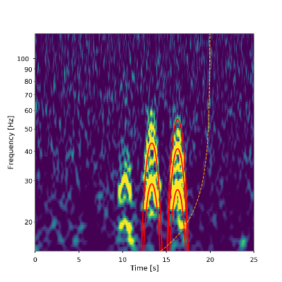
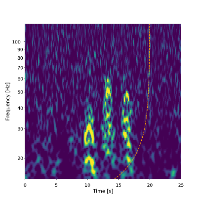
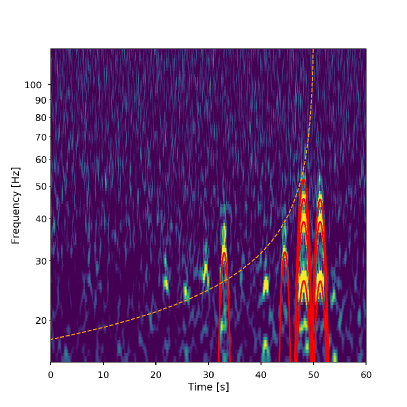
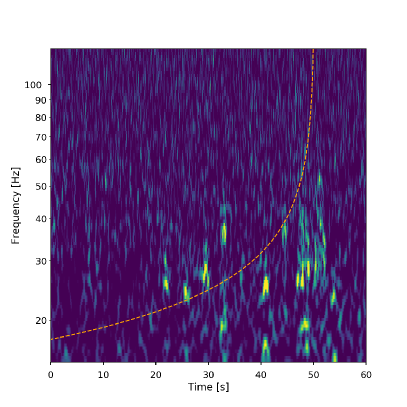
Figure 12: Two examples of gravitational wave injections found by the glitch-subtracted search for gravitational waves which were not found by the original gravitational wave search due to the presence of scattered-light glitches at the same time as the gravitational wave inspiral. Top left: A binary black hole injection with a false-alarm rate of 1 per $8643.73$ years is shown alongside the scattered-light glitches found by the ArchEnemy search and subtracted from the data prior to performing the glitch-subtracted PyCBC search for gravitational waves (top right). Bottom left: A neutron star black hole injection with a false-alarm rate of 1 per $9961.55$ years and the scattered-light glitches found by the ArchEnemy search and subtracted from the data prior to performing the glitch-subtracted PyCBC search for gravitational waves (bottom right).

To quantify the sensitivity of the search we calculate the sensitive volume in which we can observe gravitational wave signals. To calculate the sensitive volume we measure the detection efficiency of different distance bins taken from the injection sets and then multiply the efficiencies by the volume enclosed by the distance bins, these volumes are then summed to find the total volume the search is sensitive to [38]. We are then able to calculate the ratio in sensitivities between the glitch-subtracted gravitational wave search and the original gravitational wave search, revealing the improvement that subtracting scattered-light glitches has made.

Figure 13 displays the ratio of the sensitive volume measured for the glitch-subtracted gravitational wave search and the original PyCBC gravitational wave search, across different false-alarm rate values, we quote our sensitivity ratios at a false-alarm rate value of 2 per year. The same set of injected signals was used for both gravitational wave searches and therefore a direct comparison of search sensitivities can be made via this ratio. Disappointingly, the measured sensitivity improvement is small in the results we obtain. For the binary black hole injections we measure a sensitivity ratio at a 2 per year false-alarm rate of $1.01$, for binary neutron stars $1.00$ and neutron-star–black-holes $1.00$.

The statistical significance of the sensitivity increase we report for the binary black hole injection set can be found by investigating the null hypothesis of seeing the same $1\%$ increase under the assumption that the subtraction of scattered-light glitches does not actually increase sensitivity. When performing this analysis we find that our result is not statistically significant at the 95% confidence interval –i.e. there is a 5.24% chance that we would measure such an increase in sensitivity at least as large as this under the null hypothesis– (see A for details). However, the marginal sensitivity increase would not justify repeating the scattered-light glitch search and glitch-subtracted gravitational wave search on a larger injection set, instead more work is needed to better identify and remove scattered-light glitches while remaining safe in the presence of gravitational wave signals.

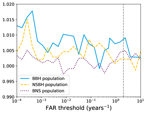
Figure 13: The ratio of the sensitive volume-time of the glitch-subtracted search and the original gravitational wave search. The grey dashed line indicates a false-alarm rate of $2$ per year which is our threshold and the point at which we measure any sensitivity improvements of the glitch-subtracted search for each of the three gravitational wave injection sets.

5 Conclusion

We have demonstrated a new method for modelling scattered-light glitches and identifying and characterizing these glitches in a period of gravitational wave data. We have developed a scattered-light glitch specific $\chi^{2}$ test which can discriminate between scattered-light glitches, other types of glitches and gravitational wave signals. We have searched through a representative stretch of gravitational wave data known to contain scattered-light glitches, found thousands of these glitches and subtracted them from the gravitational wave data prior to running a search for gravitational waves. The results of this search include a small increase in the measured sensitivity of the gravitational wave search for binary black hole gravitational wave signals, and modest change to sensitivity for binary neutron star and neutron star black hole gravitational wave signals.

We highlight that the task of accurately identifying and parameterizing scattered-light glitches in the data is not a trivial one, especially where there are repeated, and harmonic, glitches present in the data. We have developed a new $\chi^{2}$ test to reduce the number of false identifications of scattered-light glitches, but we do still see cases where we have misidentified other glitches, and even a small number of loud gravitational wave signals, as caused by scattered light, and cases where we do not correctly identify, or parameterize, actual scattered-light glitches. Improving this identification process would be important in improving the efficacy of this process.

The possibility of using this model of scattered-light glitches as a bespoke application to gravitational wave signals which are known to have coincident scattered-light glitches has been explored and implemented into Bilby [42] to perform a parameter estimation of scattered-light glitches and removing these to produce glitch-free data [43]. The inclusion of the extra term from [32] within the model can help identify scattered-light glitches more accurately. Selectively subtracting glitches based on the presence of a gravitational wave signal is possible by moving the glitch subtraction process inside of the gravitational wave searches and including the results of other gravitational wave discriminators [38, 39] to determine the legitimacy of an ArchEnemy identified glitch.

The results of the application of the ArchEnemy search pipeline, the list of scattered-light glitches, can also be used in other applications. For example it could be used in the form of a veto [14], where we use knowledge of the presence of scattered-light glitches to down rank periods of time in gravitational wave data. Additionally, we could use scattered-light glitches previously identified by tools such as Gravity Spy [22] and target known scattered-light glitches with the ArchEnemy search pipeline.

As a final note, while we acknowledge that the sensitivity improvements that we have observed—$\sim 1\%$—are very modest, the concept of removing scattered-light glitches, or other identified glitch classes, from the data prior to matched filtering for compact binary mergers is one that we encourage others to explore further. An increase in the rate of events or the rate of scattered-light glitches in future observing runs will mean an increase in the number of affected events, such techniques offer a method for mitigating the effect that these glitches will have on the search, maximizing the number of observations that can be made.

Appendix A Statistical Significance

We report a $1\%$ increase in the sensitivity for the binary black hole injection set in the glitch-subtracted gravitational wave search (see section 4). We wish to determine the statistical significance of this result under the null hypothesis that subtracting scattered-light glitches prior to searching for gravitational waves does not increase the sensitivity of the gravitational wave search. The binary black hole injection set contains $6200$ injected signals, $10$ additional injections were found in the glitch-subtracted gravitational wave search, $3$ additional injections were missed in our search, this gives us $13$ injections which have changed state.

First, we calculate the probability that an injection has been affected by the glitch removal,

$$p=\frac{13}{6200}=0.21\%,$$ (25)

then we calculate the standard deviation,

$$\textrm{std}=\sqrt{n*p*(1-p)}=3.60.$$ (26)

Using the standard deviation we calculate the number of standard deviations our result deviates from the mean. We divide the number of positively changed (newly-found) injections by the standard deviation,

$$\textrm{standard deviations}=\frac{(10-3)}{3.60}=1.94.$$ (27)

Under the assumption of no sensitivity increase caused by the subtraction of glitches, we measure our result of +7 newly-found gravitational wave injections to lie $1.94$ standard deviations from an expected value of $0$ newly-found injections. The critical value of a 95% confidence interval, that is to say there is a 1 in 20 chance of our null hypothesis being true, is $1.96$ meaning our result is within the 95% confidence interval. We can describe this as there being a 5.24% chance that our result is not caused by the subtraction of glitches but is instead caused by random chance. To reduce the error in the computed sensitivity ratio a larger injection set test would be required, this would need a large time and computational power investment which we do not believe is justified in the case of such a minor increase in the sensitivity.

Appendix B

Here we have three tables which contain data on the newly-found and newly-missed injections for each injection set. The tables are separated into the values for the inverse false-alarm rate and ranking statistic found for each injection in both searches then the signal-to-noise ratio, $\chi^{2}$ and PSD variation values for each detector in both searches. The first table is the results of the binary black hole injection set, the second table is the binary neutron star injection set and the third is the neutron star black hole injection set. A horizontal dashed line separates newly-found and newly-missed injections, using a false-alarm rate threshold of 2 per year. There were 2 newly-found binary black hole injections which were not found at all by the original search and therefore they do not appear in the first table.

There have been 34 newly-found or newly-missed gravitational wave injections when subtracting scattered-light glitches, it is informative to understand how the gravitational wave search is influenced by the glitch subtraction to cause this outcome. The ranking statistic [Davies:2020tsx] represents the legitimacy of a signal being astrophysical in origin and is partially computed using the re-weighted signal-to-noise ratio, which is itself computed using the initial signal-to-noise ratio alongside the various gravitational wave discriminators and the PSD variation measurement [40]. We use the trigger information saved by the gravitational wave search to identify why injections that weren’t found previously have been found post-glitch subtraction, and vice versa.

As an example, we take the smallest false-alarm rate (1 per $8643.73$ years), newly-found, binary black hole injection, and look at the ranking statistic, signal-to-noise ratio, $\chi^{2}$ and, PSD variation measurements in both detectors and both searches – these values can be found in table 3. This injection was originally seen with a false-alarm rate of 100 per year, far above our threshold, a very large increase in the ranking statistic from 13.29 to 27.01 is certainly responsible for the decreased false-alarm rate. There were no changes in the values measured by the LIGO-Livingston detector between searches which is expected as no scattered-light glitches were found within $512$ seconds of the injection. The LIGO-Hanford detector sees a small increase in the signal-to-noise ratio measured, from 7.98 to 8.22, a small increase in the $\chi^{2}$ value, from 2.32 to 2.48, and a very significant decrease in the PSD variation measurement, from 3.47 to 1.50. Using equation 18 of [40], we can calculate a re-weighted signal-to-noise ratio of $4.60$ for the original search and $5.67$ for the glitch-subtracted search, a significant increase in the signal-to-noise ratio. Similar analyses for all the newly-found and newly-missed injections can be made using information found in tables 4 and 5.

The decrease in the PSD variation is true for the three newly-found very low false-alarm rate injections, accompanied by the small changes in signal-to-noise ratio and increase in the $\chi^{2}$ measurement. For newly-found and newly-missed injections which lie close to the 2 per year false-alarm rate threshold there is no definitive reason as to why these injections changed state.

Table 3: This table contains the trigger information for the newly-found and newly-missed binary black hole injections recorded by the original search [8] and the glitch-subtracted search.

Glitch-Subtracted								Original Search
		H1			L1					H1			L1
IFAR	Ranking	SNR	$\chi^{2}$	PSD	SNR	$\chi^{2}$	PSD	IFAR	Ranking	SNR	$\chi^{2}$	PSD	SNR	$\chi^{2}$	PSD
	Stat.			Var.			Var.		Stat.			Var.			Var.
8643.73	27.01	8.22	2.48	1.50	8.05	2.07	1.00	0.01	13.29	7.98	2.32	3.47	8.05	2.07	1.00
7633.84	26.13	8.18	2.25	1.22	7.58	1.46	1.03	0.37	16.63	8.19	1.87	2.17	7.59	1.45	1.02
4.89	19.06	7.23	1.88	0.97	10.34	3.15	1.05	1.56	18.01	7.24	2.11	0.97	10.34	3.42	1.04
3.14	18.65	5.89	1.54	1.01	8.86	2.40	1.09	1.52	17.99	5.89	1.54	1.01	8.86	2.40	1.09
2.75	18.53	8.50	1.63	0.99	6.80	1.37	1.05	1.51	17.98	8.51	1.56	0.98	6.80	1.37	1.05
2.39	18.41	7.83	2.00	1.01	8.41	3.41	1.02	1.06	17.65	7.81	2.14	1.01	8.41	3.41	1.02
2.18	18.32	7.02	1.90	1.02	6.35	2.15	1.01	1.79	18.14	7.05	1.92	1.02	6.35	2.16	1.01
2.01	14.11	7.94	1.89	1.01	5.67	1.95	1.16	1.90	14.14	7.94	1.90	1.01	5.07	0.00	1.02
1.76	18.12	6.89	1.43	1.02	6.76	2.59	0.97	3.33	18.71	6.86	1.82	1.02	6.68	2.53	0.97
1.79	18.14	6.40	1.69	1.02	7.56	2.01	1.01	2.05	18.27	6.40	1.69	1.02	7.56	2.00	1.01
1.65	18.06	5.14	0.00	0.91	7.57	1.57	1.02	2.05	18.27	5.14	0.00	0.91	7.57	1.57	1.02

Table 4: This table contains the trigger information for the newly-found and newly-missed binary neutron star injections recorded by the original search [8] and the glitch-subtracted search.

Glitch-Subtracted								Original Search
		H1			L1					H1			L1
IFAR	Ranking	SNR	$\chi^{2}$	PSD	SNR	$\chi^{2}$	PSD	IFAR	Ranking	SNR	$\chi^{2}$	PSD	SNR	$\chi^{2}$	PSD
	Stat.			Var.			Var.		Stat.			Var.			Var.
5.12	19.12	5.86	1.99	1.01	7.15	1.94	1.02	1.49	17.96	5.74	2.14	1.01	7.15	1.94	1.02
4.91	19.07	5.48	2.29	1.01	7.92	2.16	1.01	1.37	17.89	5.78	2.25	1.01	7.23	2.13	1.01
4.54	18.99	4.82	0.00	1.07	8.68	2.05	1.06	1.66	18.07	4.82	0.00	1.14	8.68	2.05	1.06
2.46	18.43	5.48	1.95	1.05	7.61	2.03	0.99	1.78	18.13	5.48	1.94	1.05	7.62	2.08	0.99
2.34	18.39	6.25	2.18	1.01	6.82	1.96	1.00	1.45	17.94	6.09	2.05	1.01	6.83	2.01	1.00
1.24	17.71	6.58	2.14	1.01	6.89	2.48	1.01	17.81	20.19	6.58	2.15	1.01	7.16	2.26	1.01
1.14	17.72	6.00	2.67	0.98	8.07	2.66	1.22	7.14	19.44	6.17	2.45	0.97	8.26	2.80	1.22
1.89	18.19	6.32	2.19	1.00	6.79	1.83	0.99	3.57	18.78	6.37	2.12	0.99	6.79	1.75	0.99
0.88	17.46	6.88	2.14	0.99	6.19	2.12	0.99	2.33	18.39	6.87	2.07	0.99	6.19	1.99	0.99
1.36	17.80	6.20	2.02	1.00	6.83	2.35	1.00	2.07	18.18	6.20	2.02	1.00	6.83	2.28	1.00

Table 5: This table contains the trigger information for the newly-found and newly-missed neutron star black hole injections recorded by the original search [8] and the glitch-subtracted search.

Glitch-Subtracted								Original Search
		H1			L1					H1			L1
IFAR	Ranking	SNR	$\chi^{2}$	PSD	SNR	$\chi^{2}$	PSD	IFAR	Ranking	SNR	$\chi^{2}$	PSD	SNR	$\chi^{2}$	PSD
	Stat.			Var.			Var.		Stat.			Var.			Var.
9961.55	27.41	5.55	2.08	1.23	10.26	2.27	1.12	0.01	12.83	6.01	2.39	2.25	8.54	2.37	1.12
141.35	22.28	7.76	2.20	1.02	6.54	2.35	1.01	1.21	17.77	7.83	1.94	1.02	7.29	2.50	1.00
18.26	20.36	5.94	2.20	1.09	6.02	1.99	1.10	1.29	17.82	5.74	2.05	1.09	6.27	2.10	1.18
17.12	20.29	7.64	2.00	1.11	6.66	2.15	1.05	1.37	17.89	7.36	2.35	1.11	6.66	2.15	1.05
12.94	20.03	6.52	1.79	1.07	7.31	2.32	1.13	1.96	18.23	6.57	1.85	1.20	7.31	2.32	1.13
7.12	19.42	5.13	0.00	1.05	8.33	2.08	1.04	0.03	14.23	5.30	2.16	1.05	7.44	2.43	1.04
3.61	18.77	5.80	2.01	1.02	7.43	1.88	0.93	1.81	18.15	5.80	2.01	1.02	7.43	1.97	0.93
2.15	18.22	7.41	2.04	1.02	5.57	2.03	1.03	0.00	4.34	5.64	2.18	0.98	5.04	-0.00	1.01
0.23	16.16	5.79	1.81	0.96	8.78	3.93	1.03	11.69	19.93	5.78	1.89	0.96	8.79	3.17	1.03
1.56	17.92	6.71	1.91	0.99	6.73	2.50	1.05	2.68	18.41	6.71	1.90	0.99	6.72	2.39	1.05
1.72	18.10	5.77	1.90	0.99	6.77	1.74	1.00	2.08	18.28	5.77	1.90	0.99	6.80	1.69	1.00

References

- [1] Aasi J et al. (LIGO Scientific) 2015 Class. Quant. Grav. 32 074001 (Preprint 1411.4547)
- [2] Acernese F et al. (VIRGO) 2015 Class. Quant. Grav. 32 024001 (Preprint 1408.3978)
- [3] Abbott B P et al. (LIGO Scientific, Virgo) 2016 Phys. Rev. Lett. 116 061102 (Preprint 1602.03837)
- [4] Akutsu T et al. (KAGRA) 2021 Overview of KAGRA: Detector design and construction history (Preprint 2005.05574)
- [5] Abbott B P et al. (LIGO Scientific, Virgo) 2019 Phys. Rev. X 9 031040 (Preprint 1811.12907)
- [6] Abbott R et al. (LIGO Scientific, Virgo) 2021 Phys. Rev. X 11 021053 (Preprint 2010.14527)
- [7] Abbott R et al. (LIGO Scientific, VIRGO) 2021 GWTC-2.1: Deep Extended Catalog of Compact Binary Coalescences Observed by LIGO and Virgo During the First Half of the Third Observing Run (Preprint 2108.01045)
- [8] Abbott R et al. (LIGO Scientific, VIRGO, KAGRA) 2021 (Preprint 2111.03606)
- [9] Usman S A et al. 2016 Class. Quant. Grav. 33 215004 (Preprint 1508.02357)
- [10] Cannon K et al. 2020 GstLAL: A software framework for gravitational wave discovery (Preprint 2010.05082)
- [11] Chu Q et al. 2022 SPIIR online coherent pipeline to search for gravitational waves from compact binary coalescences (Preprint 2011.06787)
- [12] Aubin F et al. 2021 Class. Quant. Grav. 38 095004 (Preprint 2012.11512)
- [13] Abbott B P et al. (LIGO Scientific, Virgo) 2020 Class. Quant. Grav. 37 055002 (Preprint 1908.11170)
- [14] Davis D et al. (LIGO) 2021 Class. Quant. Grav. 38 135014 (Preprint 2101.11673)
- [15] Acernese F et al. (Virgo) 2022 (Preprint 2210.15633)
- [16] Abbott B P et al. (LIGO Scientific, Virgo) 2016 Class. Quant. Grav. 33 134001 (Preprint 1602.03844)
- [17] Buikema A et al. (aLIGO) 2020 Phys. Rev. D 102 062003 (Preprint 2008.01301)
- [18] Mukherjee S, Obaid R and Matkarimov B 2010 J. Phys. Conf. Ser. 243 012006
- [19] Cabourn Davies G S and Harry I W 2022 Class. Quant. Grav. 39 215012 (Preprint 2203.08545)
- [20] Zevin M et al. 2017 Class. Quant. Grav. 34 064003 (Preprint 1611.04596)
- [21] Soni S et al. 2021 Class. Quant. Grav. 38 195016 (Preprint 2103.12104)
- [22] Glanzer J et al. 2022 (Preprint 2208.12849)
- [23] Soni S et al. (LIGO) 2020 Class. Quant. Grav. 38 025016 (Preprint 2007.14876)
- [24] Goetz E 2021 gwdetchar/gwdetchar: 2.0.5 URL https://doi.org/10.5281/zenodo.5722057
- [25] Accadia T et al. 2010 Class. Quant. Grav. 27 194011
- [26] Davis D, Littenberg T B, Romero-Shaw I M, Millhouse M, McIver J, Di Renzo F and Ashton G 2022 Class. Quant. Grav. 39 245013 (Preprint 2207.03429)
- [27] Nuttall L K 2018 Phil. Trans. Roy. Soc. Lond. A 376 20170286 (Preprint 1804.07592)
- [28] Bianchi S, Longo A, Valdes G, González G and Plastino W 2022 Class. Quant. Grav. 39 195005 (Preprint 2107.07565)
- [29] Valdes G, O’Reilly B and Diaz M 2017 Class. Quant. Grav. 34 235009
- [30] Longo A, Bianchi S, Plastino W, Arnaud N, Chiummo A, Fiori I, Swinkels B and Was M 2020 Class. Quant. Grav. 37 145011 (Preprint 2002.10529)
- [31] Longo A, Bianchi S, Valdes G, Arnaud N and Plastino W 2022 Class. Quant. Grav. 39 035001 (Preprint 2112.06046)
- [32] Was M, Gouaty R and Bonnand R 2021 Class. Quant. Grav. 38 075020 (Preprint 2011.03539)
- [33] Allen B, Anderson W G, Brady P R, Brown D A and Creighton J D E 2012 Phys. Rev. D 85 122006 (Preprint gr-qc/0509116)
- [34] Harry I W, Allen B and Sathyaprakash B S 2009 Phys. Rev. D 80 104014 (Preprint 0908.2090)
- [35] Barsotti L, Fritschel P, Evans M and Slawomir G 2018 Updated advanced ligo sensitivity design curve URL https://dcc.ligo.org/LIGO-T1800044/public
- [36] Abbott R et al. (LIGO Scientific, Virgo) 2021 SoftwareX 13 100658 (Preprint 1912.11716)
- [37] Allen B 2005 Phys. Rev. D 71 062001 (Preprint gr-qc/0405045)
- [38] Abadie J et al. (LIGO Scientific, VIRGO) 2012 Phys. Rev. D 85 082002 (Preprint 1111.7314)
- [39] McIsaac C and Harry I 2022 Phys. Rev. D 105 104056 (Preprint 2203.03449)
- [40] Mozzon S, Nuttall L K, Lundgren A, Dent T, Kumar S and Nitz A H 2020 Class. Quant. Grav. 37 215014 (Preprint 2002.09407)
- [41] Abadie J et al. (LIGO Scientific, VIRGO) 2012 Phys. Rev. D 85 082002 (Preprint 1111.7314)
- [42] Ashton G et al. 2019 Astrophys. J. Suppl. 241 27 (Preprint 1811.02042)
- [43] Udall R and Davis D 2022 (Preprint 2211.15867)