End benches scattered light modeling and subtraction in Advanced Virgo

Abstract

Advanced Virgo end benches were a significant source of scattered light noise during the third observing run that lasted from April 1 2019 until March 27 2020. We describe how that noise could be subtracted using auxiliary channels during the online strain data reconstruction. We model in detail the scattered light noise coupling and demonstrate that further noise subtraction can be achieved. We also show that the fitted model parameters can be used to optically characterized the interferometer and in particular provide a novel way of establishing an absolute calibration of the detector strain data.

1 Introduction

Interferometric gravitational wave detectors have their sensitivity affected by scattered light, especially when microseism ground motion is elevated at times of rough seas. Examples of ground motion coupling to the sensitivity of detectors through scattered light have been previously described for initial Virgo [1, 2], GEO-HF [3] and most recently advanced LIGO [4, 5].

In this paper we focus on the coupling of light scattered by the end suspended benches to the sensitivity of Advanced Virgo. This was a significant source of scattered light noise during the third observing run (O3) that lasted from April 1 2019 until March 27 2020. However, it was sufficiently well measured that scattered light noise could be subtracted after the fact from the gravitational wave strain data.

This paper is organized as follows. In section 2 we describe the theory of scattered light coupling from the suspended benches, in section 3 we show that scattered light can be measured using photodiodes located on these benches, in section 4 we demonstrate how these signals can be used to subtract scattered light noise from the strain data, and in section 5 we propose how to use scattered light as a new method to calibrate the strain data.

2 End benches scattered light theory

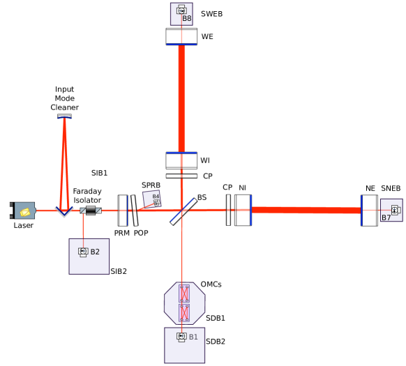
Figure 1: Optical layout of Advanced Virgo during O3, adapted from [6] with kind permission of The European Physical Journal (EPJ).

A simplified optical layout of Advanced Virgo during O3 is shown on figure 1. It is a power recycled Fabry-Perot Michelson interferometer with 3 km arms. The interferometer transforms gravitational wave strain into audio frequency power fluctuations on the anti-symmetric port photodiode denoted B1. In transmission of the north end (NE) mirror and respectively the west end (WE) mirror are located the suspended north end bench (SNEB) and respectively the suspended west end bench (SWEB). Each of these benches host among others a photodiode denoted respectively B7 and B8.

Let $E_{0}$ be the electromagnetic field inside the west Fabry-Perot cavity at the highly reflective (HR) surface of the WE mirror of power transmission $T_{\text{WE}}\simeq 4.3\times 10^{-6}$ [7], and $x$ be the distance between that surface and the scattering surface located on SWEB which reflects a fraction $f_{r}$ of the impinging light. The electromagnetic field inside the Fabry-Perot cavity is in the fundamental Gaussian transverse mode, hence the field forward propagating on the bench is also in this mode, in particular light reaching photo-diodes. On the contrary light is scattered at all angles, the fraction $f_{r}$ considers only the small portion of scattered light that is back scattered in the fundamental Gaussian mode and mode matched with the light inside the Fabry-Perot cavity. This is the only scattered light which will efficiently interfere with the dominant field in the arm cavities and on the photodiodes. As $T_{\text{WE}}$ and $f_{r}$ are small in the following we will keep only the leading term in $\sqrt{T_{\text{WE}}}$ and $\sqrt{f_{r}}$.

The scattering surface create a field $E_{\text{sc}}$ that at the HR surface of the WE mirror is

$$E_{\text{sc}}=\sqrt{T_{\text{WE}}f_{r}}E_{0}e^{i\phi_{\text{sc}}},$$ (1)

where $\phi_{\text{sc}}=4\pi\frac{x}{\lambda}$ is the phase delay due to the round trip propagation and $\lambda$ is the laser wavelength. A small fraction of that light is transmitted through the HR coating yielding a total field

$$E_{\text{tot}}=E_{0}+\sqrt{T_{\text{WE}}}E_{\text{sc}}=E_{0}\left(1+T_{\text{WE}}\sqrt{f_{r}}e^{i\phi_{\text{sc}}}\right),$$ (2)

while the majority is reflected back yielding a field $E_{\text{B8}}$ towards the B8 photodiode

$$E_{\text{B8}}=\sqrt{T_{\text{WE}}}E_{0}+E_{\text{sc}}=\sqrt{T_{\text{WE}}}E_{0}\left(1+\sqrt{f_{r}}e^{i\phi_{\text{sc}}}\right).$$ (3)

The field perturbation inside the arm cavity is amplified by the Fabry-Perot cavity in a frequency dependent way by

$$G(f)=\frac{1}{1-r}\frac{1}{1+i\frac{f}{f_{\text{arm}}}},$$ (4)

where $r=\sqrt{1-T_{\text{WI}}-\Lambda_{\text{arm}}}\sim 0.993$ [8] is the effective field reflectivity of the WI mirror taking into account the arm cavity round trip losses $\Lambda_{\text{arm}}$,

$$f_{\text{arm}}=\frac{1-r}{r}\frac{c}{4\pi L}\simeq 55\,{\rm Hz}$$ (5)

is the arm cavity pole frequency and $L=3$ km is the arm cavity length. This yields a field inside the cavity

$$E_{\text{cavity}}=E_{0}\left(1+GT_{\text{WE}}\sqrt{f_{r}}e^{i\phi_{\text{sc}}}\right).$$ (6)

The interferometer is operated in DC read-out [9, 10] with an offset in the differential arm length. Let us denote $\psi$ the differential phase offset and $h$ the amplitude of a putative gravitational wave. The field inside the cavities becomes

$$E_{\text{cavity, west}} = E_{0}e^{i\left(\frac{\psi}{2}+2\pi G\frac{hL}{\lambda}\right)}\left(1+GT_{\text{WE}}\sqrt{f_{r}}e^{i\phi_{\text{sc}}}\right)$$ (7)

$$E_{\text{cavity, north}} = E_{0}e^{-i\left(\frac{\psi}{2}+2\pi G\frac{hL}{\lambda}\right)}$$ (8)

where $L$=3 km is the cavity length. A fraction $T_{\text{IM}}=0.0138$ [8] of these fields returns through the input mirrors and recombines at the beam splitter, which yield at the anti-symmetric port of the interferometer a power

$$P_{\text{B1}} = T_{\text{IM}}\left|E_{\text{cavity, west}}-(1-\epsilon)E_{\text{cavity, north}}\right|^{2}$$

$$= T_{\text{IM}}|E_{0}|^{2}\left[\psi^{2}+\epsilon^{2}+2\psi 4\pi G\frac{hL}{\lambda}+\right.$$

$$\left.2\psi GT_{\text{WE}}\sqrt{f_{r}}\sin\phi_{\text{sc}}+2\epsilon GT_{\text{WE}}\sqrt{f_{r}}\cos\phi_{\text{sc}}\right],$$

where $\epsilon$ accounts for asymmetries between the two arms that yield a contrast defect of the interferometer.

Thus scattered light directly mimicks a gravitational wave signal through phase and amplitude coupling

$$h_{\text{sc, phase}} = \frac{1}{L}T_{\text{WE}}\sqrt{f_{r}}\frac{\lambda}{4\pi}\sin\phi_{\text{sc}}$$ (9)

$$h_{\text{sc, amplitude}} = \frac{\epsilon}{\psi}\frac{1}{L}T_{\text{WE}}\sqrt{f_{r}}\frac{\lambda}{4\pi}\cos\phi_{\text{sc}}.$$ (10)

However, there are additional coupling path as scattered light modulates the power inside the west arm cavity

$$P_{\text{cavity}}=|E_{0}|^{2}\left(1+2GT_{\text{WE}}\sqrt{f_{r}}\cos\phi_{\text{sc}}\right),$$ (11)

which through radiation pressure displaces in opposite directions the WI and WE mirrors and create an additional spurious signal

$$h_{\text{sc, pressure}} = \frac{2}{L}\frac{2\delta P_{\text{cavity}}}{c}\text{WE}_{F\rightarrow z}$$ (12)

$$= \frac{G}{L}\text{WE}_{F\rightarrow z}\frac{8|E_{0}|^{2}}{c}T_{\text{WE}}\sqrt{f_{r}}\cos\phi_{\text{sc}},$$ (13)

where $c$ is the speed of light and

$$\text{WE}_{F\rightarrow z}(f)=\frac{1}{M}\frac{1}{\Omega^{2}-(2\pi f)^{2}}$$ (14)

is the mechanical response of the suspended WE mirror with $M$ the mass of the mirror and $\Omega$ the mirror suspension pendulum angular frequency. Note that we omit here optical spring effects that have a negligible effect above 10 Hz as shown by the comparison to numerical simulation described at the end of this section.

These power fluctuations are further amplified and filtered in the combined power recycling and arm cavity by

$$G_{\text{combined}}(f)=\frac{\sqrt{T_{\text{IM}}}}{(1-r)(1-r_{\text{PR}})+r_{\text{PR}}\Lambda_{\text{arm}}}\frac{1}{1+i\frac{f}{f_{\text{combined}}}},$$ (15)

where $r_{\text{PR}}=\sqrt{1-T_{\text{PR}}-\Lambda_{\text{PR}}}=0.975$ [11] is the effective field reflectivity of the PR mirror taking into account the power recycling cavity round trip losses $\Lambda_{\text{PR}}$ and

$$f_{\text{combined}}=\frac{(1-r)(1-r_{\text{PR}})+r_{\text{PR}}\Lambda_{\text{arm}}}{r+r_{\text{PR}}-\Lambda_{\text{arm}}}\frac{c}{4\pi L}\simeq 1.0\,{\rm Hz}$$ (16)

is the combined cavity pole frequency. The displacement caused by the radiation pressure of these fluctuations is common to both arms, hence a priori the lengths of both arms is changed by the same amount not yielding any differential signal. However the power in the arms is not exactly equal, it may differ by a small fraction $\rho$, which will yield a differential effect as radiation pressure displacement is proportional to the power in the given arm. This creates a spurious signal

$$h_{\text{sc, pressure recycled}}=\rho\sqrt{T_{\text{WI}}}\frac{G_{\text{combined}}}{2}h_{\text{sc, pressure}},$$ (17)

where the factor $\frac{1}{2}$ accounts for the recycled power being split between the two arms.

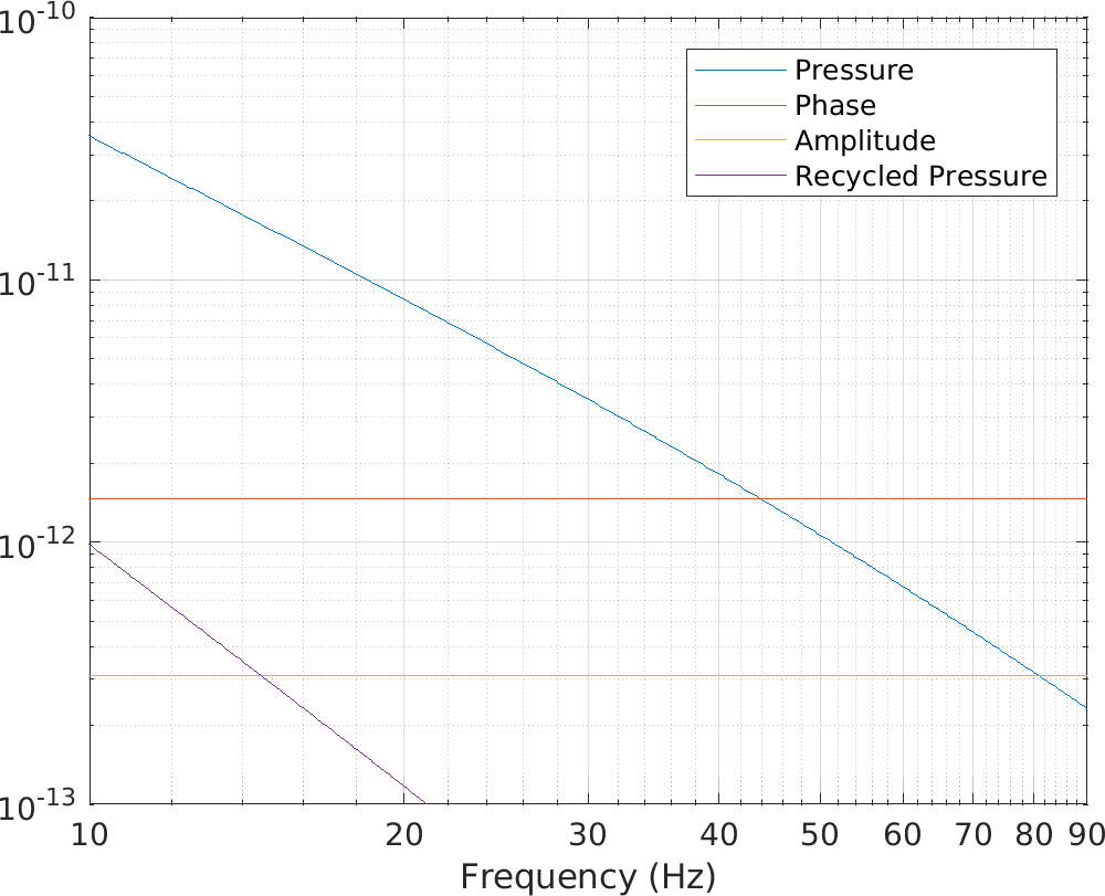
Figure 2: Left pane shows the scattering coupling transfer functions for the three coupling paths: radiation pressure given by equation (13), phase given by equation (9), amplitude given by equation (10), and recycled radiation pressure given by equation (17). The right pane shows the ratio between the transfer function numerically computated using Optickle and the analytical computation shown on the left pane.

The power inside the arm cavities is estimated to be $|E_{0}|^{2}=90$ kW for a laser input power of 18 W used in the first half of O3. While the dark fringe power was set to be $P_{\text{B1}}=2.8$ mW and the contrast defect light in the TEM00 mode in transmission of the output mode cleaner was measured to be $120\pm 20$ $\mu$W [12], which yields $\epsilon/\psi=0.21$. The power ratio between the two arms has not been accurately measured, but it varied by $\sim$1% during the run which sets an order of magnitude for $\rho$. These measurements allows us to evaluate the relative contributions of the four coupling paths as shown on figure 2 assuming a fiducial scattering $f_{r}=10^{-6}$. The radiation pressure is dominant below 45 Hz while the phase coupling is dominant above. Note that in a previous estimate [13] of the scattered light coupling a factor 2 was missing for the radiation pressure and phase coupling path, and the amplitude and recycled radiation pressure coupling paths were completely neglected.

These analytic computations have been verified to be accurate with an interferometer simulation performed with the Optickle simulation software [14]. The only deviation is that in simulation the radiation pressure effects include the optical spring at $\sim 4$ Hz, which causes a small deviation at low frequency of 2% in amplitude and 1 degree in phase at $10$ Hz as shown on figure 2. In the following section we use the optical simulation results scaled by the parameters derived analytically to perform fits.

Fortunately the scattered light interference also produces a signal on the B8 photodiode

$$P_{\text{B8}}=\alpha T_{\text{WE}}|E_{0}|^{2}\left(1+2\sqrt{f_{r}}\cos\phi_{\text{sc}}\right),$$ (18)

where $\alpha$ accounts for the light losses between WE and the B8 photodiode due to pick-offs for quadrant photodiodes and cameras, photodiode quantum efficiency, and other loss mechanisms. In particular the relative intensity noise (RIN) of $P_{\text{B8}}$ yields a direct measurement of the scattered light fraction

$$\frac{\delta P_{\text{B8}}}{P_{\text{B8}}}=2\sqrt{f_{r}}\cos\phi_{\text{sc}}.$$ (19)

3 Measurement of scattered light fraction

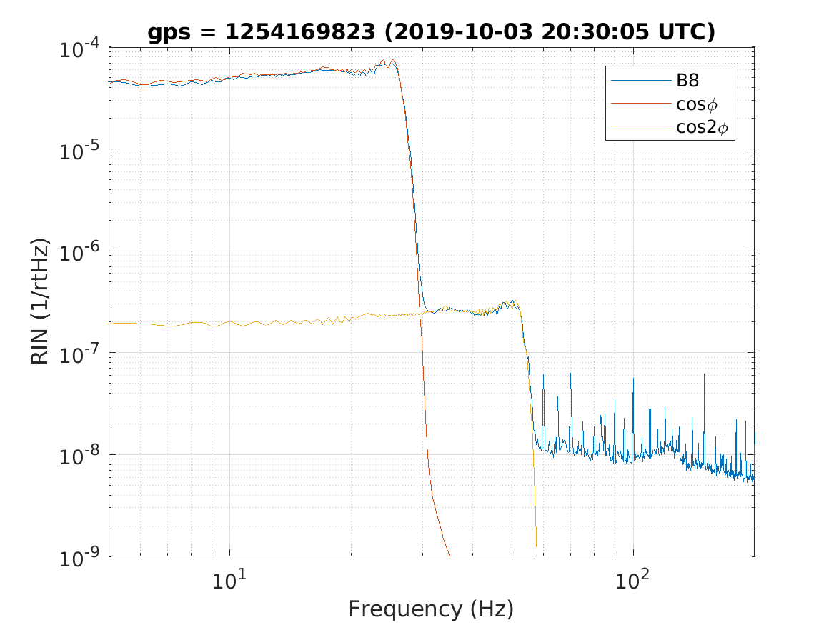
Figure 3: Relative intesity noise (RIN) of $P_{\text{B8}}$ with superposed fringe wrapped relative motion between SWEB and WE during the time of intentional SWEB motion with the quadrant shutters open.

Large amplitude slow motion of the bench, especially at the microseism peak at 300 mHz, is up converted to the sensitive band of the detector (above 10 Hz) by the sine and cosine function of $\phi_{\text{sc}}=4\pi\frac{x}{\lambda}$. This yields a noise with characteristic arch shape in a time-frequency representation of the data with a time dependent frequency $f(t)=\frac{2\left|\dot{x}(t)\right|}{\lambda}$ proportional to the bench speed. The variation in distance $x$ between SWEB and WE can be directly measured from the ground connected local controls of SWEB (linear variable differential transformers) and of WE (optical levers), where the ground motion is removed at first order by taking the difference of these sensors.

To study scattering coupling the SWEB bench has been intentionally moved with large amplitude to increase the scattered light noise signal in the detector. In total four measurements of 3 minutes in duration have been performed over a 30 minutes time span. Two with an intentional motion of SWEB and two with an intentional motion of SNEB. In each case one of the measurement was with the quadrant shutters open and one with the quadrant shutters closed.

	$f_{r}$	$f_{2r}$
SWEB, open	$4.0\times 10^{-8}$	$1.5\times 10^{-12}$
SWEB, closed	$6.0\times 10^{-9}$	$1.5\times 10^{-12}$
SNEB, open	$2.5\times 10^{-8}$	$3.0\times 10^{-14}$
SNEB, closed	$3.5\times 10^{-8}$	$5.0\times 10^{-14}$

Table 1: Fitted scattered power for four different measurements with intentional large amplitude motion of either SWEB or SNEB, and with quadrant photodiode shutters on given bench either open or closed.

Using equation (19) we fit the scattering fraction $f_{r}$ to match the RIN of $P_{\text{B8}}$. In addition, the second order scattering fraction $f_{2r}$ is clearly visible, which correspond to light that makes two round trips between the mirror and the bench. An example is shown on figure 3, and the fit parameters for all four measurements are shown in table 1.

Note that closing the quadrant shutters reduces the SWEB scattering by almost an order of magnitude from $f_{r}=4.0\times 10^{-8}$ to $f_{r}=6.0\times 10^{-9}$. When the shutters are closed the beam is dumped on anti-reflective coated black glass on the bench which has low scattering, which explains the reduction in scattering. However, for SNEB the scattering increases from $f_{r}=2.5\times 10^{-8}$ to $f_{r}=3.5\times 10^{-8}$. This is due to the lack of these beam dumps on SNEB, the beam is sent instead on the vacuum chamber wall that appears to have a scattering similar in magnitude to the back scatter from the quadrant photodiode sensor.

4 Subtraction of scattered light

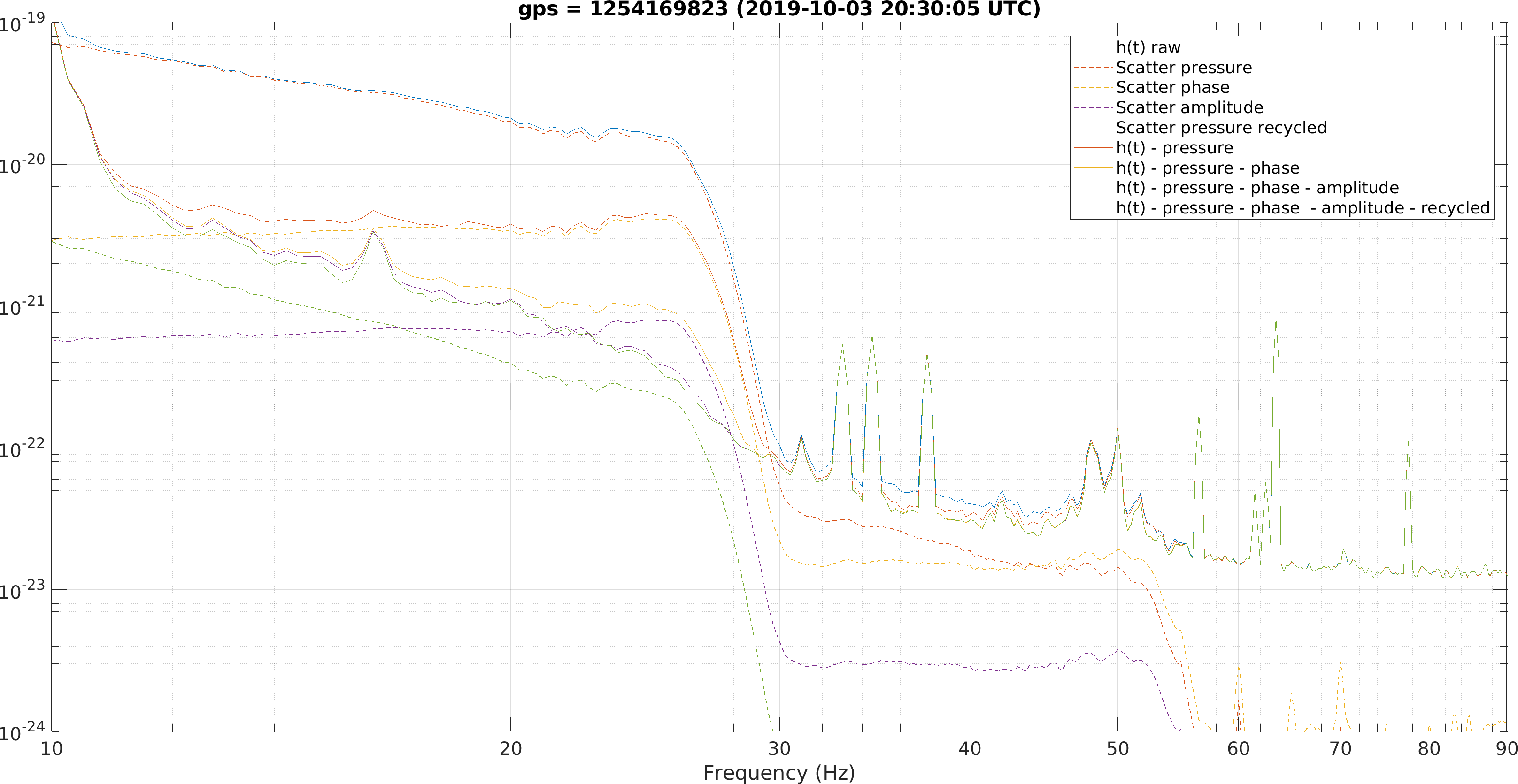
Figure 4: Spectrum of strain data during an intentional motion of SWEB. Shown are the original strain data, the projections of the radiation pressure, phase and amplitude couplings, alongside the successive subtraction in time domain of each of these contributions.

The RIN of $P_{\text{B8}}$ give us direct access to the coherent sum of $\cos\phi_{\text{sc}}$ and $\cos 2\phi_{\text{sc}}$ with the appropriate scattering fraction coefficient. In addition, the $\sin\phi_{\text{sc}}$ term which couples through (9) can be reconstructed from the Fourier decomposition of $\cos\phi_{\text{sc}}$ and the bench speed as follows

$$\cos\phi_{\text{sc}}(t) = \int_{-\infty}^{\infty}\hat{\phi}_{\text{sc}}(\omega)e^{i\omega t}\mathrm{d}\omega$$ (20)

$$\sin\phi_{\text{sc}}(t) = i\mathop{\rm sign}\left[\frac{\mathrm{d}\phi_{\text{sc}}(t)}{\mathrm{d}t}\right]\int_{0}^{\infty}\left[\hat{\phi}_{\text{sc}}(-\omega)e^{-i\omega t}-\hat{\phi}_{\text{sc}}(\omega)e^{i\omega t}\right]\mathrm{d}\omega.$$ (21)

We will not attempt a formal derivation of that relation, instead we show that it is able to coherently subtract the observed scattering noise.

In practice we use the local controls to obtain the bench speed in $\rm\mu m/s$, and use the $\tanh$ function instead of $\mathop{\rm sign}$ to avoid a discontinuity when the speed is low. For low speeds the exact value of $\sin\phi_{\text{sc}}(t)$ does not matter as its contribution will remain below 10 Hz.

We have verified that this reconstruction method of $\sin\phi_{\text{sc}}(t)$ does not introduce any bias in amplitude or phase using surrogate data as follows. We create a bench motion time series by filtering white Gaussian noise with a resonant pole at 0.1 Hz with a quality factor of 30. This yields a simulation of an imperfect intentional motion of the bench. We add a white noise 3 orders of magnitude lower than the cosine of the bench phase to simulate the sensing noise of the B8 photodiode. Using the method above we reconstruct the sine of the bench phase and compare it to the direct computation. The obtained reconstruction errors are lower than 0.1% in the 10-30 Hz band.

We then apply this $\sin\phi_{\text{sc}}(t)$ reconstruction method to the real detector data described in section 3. We use the transfer functions given by equations (9,10,13) to subtract the scattering noise measured by $P_{\text{B8}}$ and the reconstructed phase quadrature during a time of intentional motion of SWEB. The result is shown on figure 4 and demonstrate up to a factor 40 reduction in scattered light noise. Also the second order scattering between 30 Hz and 55 Hz is correctly removed. To be able to fit these theoretical transfer functions to measurements, we diagonalize the measured transfer functions using the cross correlation matrix between $\cos\phi_{\text{sc}}$ and $\sin\phi_{\text{sc}}$, as performed in gravitational wave strain noise subtractions [15].

				contrast
	$T_{\text{WE}}$	$T_{\text{NE}}$	$|E_{0}|^{2}$	defect	$\rho$
	(ppm)	(ppm)	(kW)	($\mu$W)	(%)
SWEB, open	$4.34\pm 0.04$	–	$92.1\pm 0.7$	$95\pm 8$	$1.41\pm 0.06$
SWEB, closed	$4.36\pm 0.17$	–	$92.1\pm 5.1$	$82\pm 31$	$1.73\pm 0.10$
SNEB, open	–	$4.45\pm 0.08$	$91.6\pm 1.8$	$132\pm 19$	$1.05\pm 0.17$
SNEB, closed	–	$4.46\pm 0.05$	$91.3\pm 1.2$	$180\pm 12$	$1.26\pm 0.04$
expected
[7, 16, 12]	$4.3\pm 0.2$	$4.4\pm 0.1$	$90\pm 5$	$120\pm 20$	$\sim 1$

Table 2: Fitted interferometer parameters for four different measurements with intentional large amplitude motion of either SWEB or SNEB, and with quadrant photodiodes shutters on given bench either open or closed. For comparison the expected value of these parameters from other measurements is also shown.

In total four measurements of 3 minutes in duration have been performed. Two with an intentional motion of SWEB and two with an intentional motion of SNEB. In each case one of the measurement was with the quadrants shutters open and one with the quadrants shutters closed.

To achieve this high subtraction efficiency we fitted the interferometer parameters as listed in table 2. The measurement errors were estimated by splitting the 3 minute of available data into 6 blocks of 30 seconds, and repeating the complete analysis and fit separately on each of them. However these do not include systematic errors for example due to the frequency dependent response of the photodiodes, which could add $\sim$2% errors on the leading parameters of $T_{\text{WE}}$, $T_{\text{NE}}$ and $|E_{0}|^{2}$, and potentially larger errors in the sub-dominant parameters. This is a likely explanation for the inconsistency in the measured contrast defect and arm power asymmetry $\rho$ between the SNEB and SWEB measurements.

The model and method described above have not been used to subtract scattered light noise from O3 online strain data used for gravitational wave analysis. Instead a simpler model independent approach has been used in the reconstruction process of the strain data to subtract several different noises [17]. This was performed by measuring the transfer function between auxiliary channels and the strain data over a 500 s long strech of data, and using these transfer functions on the following 500 s of data to subtract the noise from these auxiliary channels. The measured power $P_{\text{B8}}$ and $P_{\text{B7}}$ were among the auxiliary channels to subtract noise, which allowed to subtract the combined contribution of radiation pressure, recycled radiation pressure and amplitude coupling. $P_{\text{B8}}$ was more critical as the SWEB suspension suffered from a reduced isolation leading to larger motion during bad weather times.

On figure 5 we show that this noise subtraction was effective at removing the radiation pressure contribution of scattered light from SWEB that is coherent with $P_{\text{B8}}$, leading to sensitivity improvement of up to a factor 4. However that method was not able to remove the phase coupling path which is not coherent with B8. Using equation (21) to reconstruct the phase coupling we are able to reduce the noise by a further 30% at 20 Hz.

The strain data after subtraction are incoherent with the two subtracted components (proportional to $\cos\phi_{\text{sc}}$ and $\sin\phi_{\text{sc}}$), hence the residual strain data noise adds in quadrature with these components. Given the overall factor 5 decrease in noise at 20 Hz, it means that the scattered light noise measured by $P_{\text{B8}}$ has been removed with $\sim 98\%$ efficiency, consistent with the factor 40 reduction in noise observed during intentional motion of the benches.

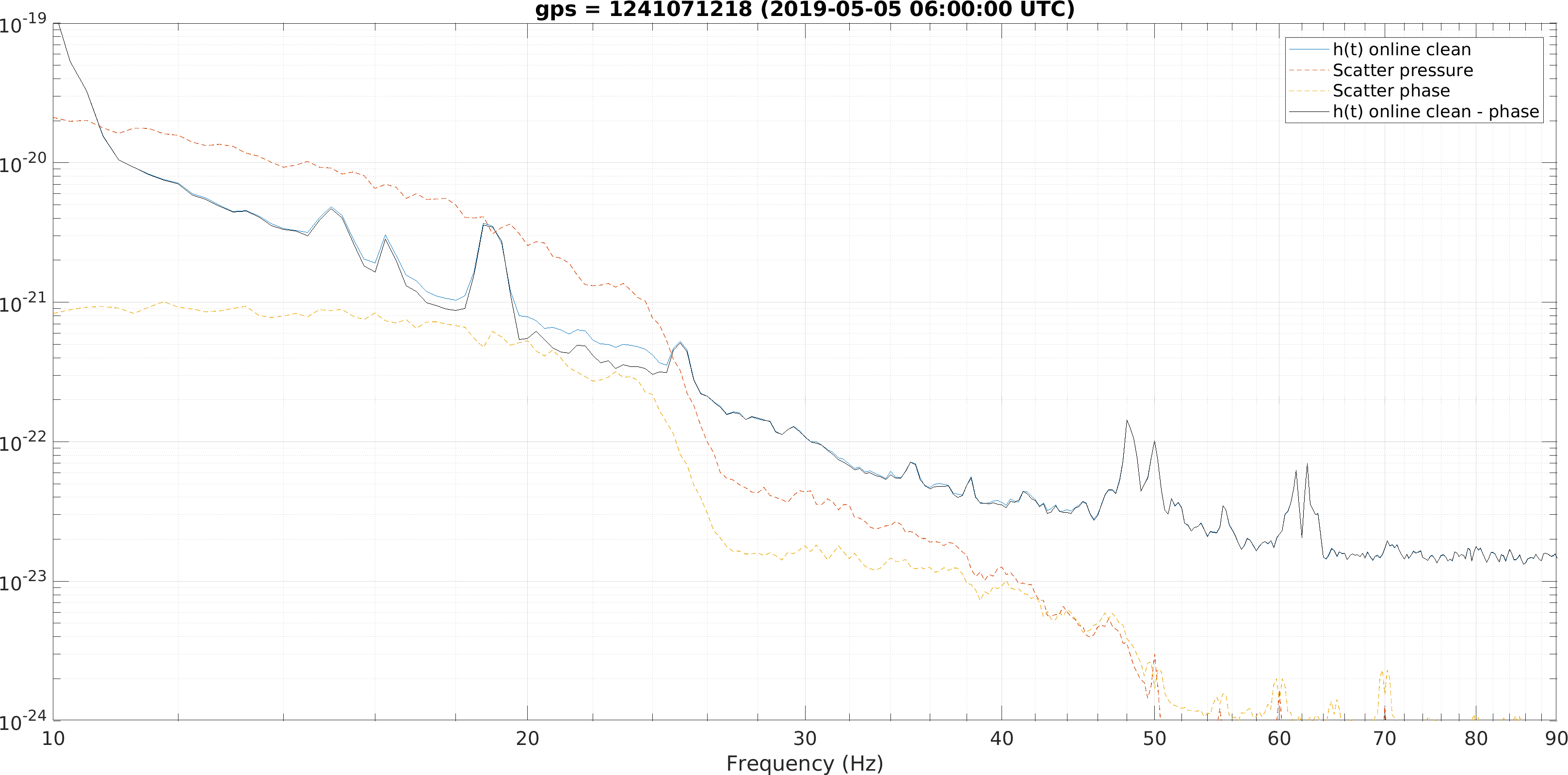
Figure 5: Spectrum of strain data during bad weather. Shown are the strain data after online noise cleaning, the projections of the radiation pressure and phase couplings of SWEB motion, and the effect of subtracting the phase coupling from the already cleaned data.

5 Interferometer absolute calibration

The measurement of $T_{\text{WE}}$ and $T_{\text{NE}}$ described above are derived from equation (9) and assumed that the calibration of the strain data was accurate. However the transmission of the end mirrors have also been measured at LMA before installation [7, 16] ($T^{\text{LMA}}_{\text{WE}}=4.3\pm 0.2\times 10^{-6}$ and $T^{\text{LMA}}_{\text{NE}}=4.4\pm 0.1\times 10^{-6}$). Comparing the two measurement of the mirror transmission yields a measurement of the accuracy of the strain data calibration.

Indeed, combining equations (9) and (19) we obtain that scattered light introduces an absolutely calibrated signal

$$h_{\text{signal}}=\frac{1}{L}T_{\text{WE}}\frac{\lambda}{4\pi}\frac{1}{2}\mathcal{TF}\left[\frac{\delta P_{\text{B8}}}{P_{\text{B8}}}\right],$$ (22)

where $\mathcal{TF}$ is the transform from to $\cos\phi_{\text{sc}}$ to $\sin\phi_{\text{sc}}$ given in equation (21). The arm length $L$ and the laser wavelength $\lambda$ are known with precision better than 0.01%, which introduces a negligible error. We also assume that the photodiode frequency response is corrected to be flat between DC and the measurement band of 10-30 Hz. In this case the ratio of the calibrated scatter light signal with the calibrated strain data after reconstruction $h_{\text{rec}}$ is directly equal to the ratio of the two estimates of the WE mirror transmissions

$$\frac{h_{\text{rec}}}{h_{\text{signal}}}=\frac{T_{\text{WE}}}{T^{\text{LMA}}_{\text{WE}}}=\frac{4.34\pm 0.04\times 10^{-6}}{4.3\pm 0.2\times 10^{-6}}=1.009\pm 0.05.$$ (23)

Analogously for the NE mirror transmission estimates yields $\frac{h_{\text{rec}}}{h_{\text{signal}}}=1.014\pm 0.025$. The dominant source of error in these measurements comes from the 2-5% uncertainty in the end mirror coating transmission, the statistical error is of the order of 1% and could be reduced by longer measurements.

The current calibration of LIGO and Virgo is performed using a photon calibrator [18, 19], an auxiliary laser that pushes on the mirrors through radiation pressure. A fundamental issue of that method is the absolute calibration of the laser power of that auxiliary laser, as the references standards in different countries are in disagreement by several percent. For O3 this has been addressed by inter-calibrating the LIGO and Virgo power references, which removes a calibration bias between the instruments but leaves the possibility of an absolute bias of the calibration of the gravitational wave detector network. The method described above could allow an absolute calibration of the detectors which do not rely on these power reference standards. Instead the method relies on precise measurement of the transmission of the end mirrors before their installation, a relative power measurement that has been performed with a few percent precision. However, in principle that precision could be significantly improved by developing the corresponding metrology.

6 Conclusions

We have shown how both quadratures of the scattered light from suspended end benches can be reconstructed from the signal of the photodiode located on that bench and from the information on the sign of the bench displacement speed. We derive a model of the main coupling mechanism for scattered light from these benches to the detector sensitivity, which allows to fit real data and subtract the scattered light noise contribution by up to a factor 40.

Moreover, the fitted interferometer parameters demonstrate how scattered light injections can be used to characterize the interferometer, as they provide self calibration injections of light field fluctuations directly into each arm cavity. In particular they are able to measure the power circulating in the interferometer and the interferometer contrast defect.

We have also shown that scattered light noise can be used to accurately calibrate the absolute response of the detector. This method is completely independent of previously proposed methods such as the “free Michelson” method [17], the photon calibrator or newtonian calibrator [20]. We stress that measurement described above was opportunistic and performed for a different purpose. Dedicated measurements would yield more robust results. For instance by performing scattered light injection over a longer time with a faster motion to cover frequencies up to at least 100 Hz, which more clearly separates the different coupling mechanism that are dominant at different frequencies.

References

References

- [1] J. Aasi et al. The characterization of Virgo data and its impact on gravitational-wave searches. Class. Quantum Grav., 29:155002, 2012.
- [2] T. Accadia et al. Noise from scattered light in Virgo’s second science run data. Class. Quantum Grav, 27:194011, 2010.
- [3] K. L. Dooley et al. GEO 600 and the GEO-HF upgrade program: successes and challenges. Class. Quantum Grav., 33:075009, 2016.
- [4] B P Abbott et al. Effects of data quality vetoes on a search for compact binary coalescences in advanced LIGO’s first observing run. Class. Quantum Grav., 35(6):065010, feb 2018.
- [5] S. Soni et al. Reducing scattered light in LIGO’s third observing run. Technical report, 2020. arXiv: 2007.14876.
- [6] F. Acernese et al. Status of advanced virgo. EPJ Web of Conferences, 182:02003, 2018.
- [7] L. Pinard. Advanced virgo end mirror characterization report- em03 (coatings c14042/20 + c14035/20). Technical report, VIR-0270A-15, 2015.
- [8] L. Pinard. Advanced virgo input mirror characterization report- im02 (coatings c14081+c14087). Technical report, VIR-0543A-14, 2014.
- [9] S. Hild et al. DC-readout of a signal-recycled gravitational wave detector. Class. Quantum Grav., 26:055012, 2009.
- [10] T. Fricke et al. DC readout experiment in Enhanced LIGO. Class. Quantum Grav., 29:065005, 2012.
- [11] L. Pinard. Advanced virgo power recycling mirror characterization report- pr01 (coatings c14097+c14101). Technical report, VIR-0029A-15, 2015.
- [12] M. Was, Virgo logbook 46956. https://logbook.virgo-gw.eu/virgo/?r=46956.
- [13] David J Ottaway, Peter Fritschel, and Samuel J. Waldman. Impact of upconverted scattered light on advanced interferometric gravitational wave detectors. Optics Express, 20(8):8329, mar 2012.
- [14] Optickle source code: https://github.com/Optickle/Optickle/tree/Optickle2.
- [15] Derek Davis, Thomas Massinger, Andrew Lundgren, Jennifer C Driggers, Alex L Urban, and Laura Nuttall. Improving the sensitivity of advanced LIGO using noise subtraction. Classical and Quantum Gravity, 36(5):055011, feb 2019.
- [16] L. Pinard. Advanced virgo end mirror characterization report- em01 (coatings c14042/10 + c14035/10). Technical report, VIR-0270A-15, 2015.
- [17] F Acernese et al. Calibration of advanced virgo and reconstruction of the gravitational wave signal h(t) during the observing run o2. Class. Quantum Grav., 35(20):205004, sep 2018.
- [18] S. Karki, D. Tuyenbayev, S. Kandhasamy, B. P. Abbott, T. D. Abbott, E. H. Anders, J. Berliner, J. Betzwieser, C. Cahillane, L. Canete, C. Conley, H. P. Daveloza, N. De Lillo, J. R. Gleason, E. Goetz, K. Izumi, J. S. Kissel, G. Mendell, V. Quetschke, M. Rodruck, S. Sachdev, T. Sadecki, P. B. Schwinberg, A. Sottile, M. Wade, A. J. Weinstein, M. West, and R. L. Savage. The advanced LIGO photon calibrators. Review of Scientific Instruments, 87(11):114503, nov 2016.
- [19] D. Estevez, P. Lagabbe, A. Masserot, L. Rolland, M. Seglar-Arroyo, and D. Verkindt. The advanced virgo photon calibrators. Technical Report VIR-0705A-20, 2020.
- [20] D Estevez, B Lieunard, F Marion, B Mours, L Rolland, and D Verkindt. First tests of a newtonian calibrator on an interferometric gravitational wave detector. Classical and Quantum Gravity, 35(23):235009, nov 2018.