Daily monitoring of scattered light noise due to microseismic variability at the Virgo interferometer

Abstract

Data acquired by the Virgo interferometer during the second part of the O3 scientific run, referred to as O3b, were analysed with the aim of characterising the onset and time evolution of scattered light noise in connection with the variability of microseismic noise in the environment surrounding the detector. The adaptive algorithm used, called pytvfemd, is suitable for the analysis of time series which are both nonlinear and nonstationary. It allowed to obtain the first oscillatory mode of the differential arm motion degree of freedom of the detector during days affected by scattered light noise. The mode’s envelope i.e., its instantaneous amplitude, is then correlated with the motion of the West end bench, a known source of scattered light during O3. The relative velocity between the West end test mass and the West end optical bench is used as a predictor of scattered light noise. Higher values of correlation are obtained in periods of higher seismic noise in the microseismic frequency band. This is also confirmed by the signal-to-noise ratio (SNR) of scattered light glitches from GravitySpy for the January-March 2020 period. Obtained results suggest that the adopted methodology is suited for scattered light noise characterisation and monitoring in gravitational wave interferometers.

1 Introduction

Virgo is a ground-based gravitational wave (GW) detector located in Cascina, near Pisa (Italy) having a detection frequency band ranging from 10 Hz to a few  kHz [1, 2]. Environmental noise characterisation and mitigation are of key importance for detectors such as Virgo. A relevant example in this regard is seismic noise, affecting the detector in the 0.1-200 Hz band [3, 4, 5, 6, 7]. In the 0.1-1 Hz frequency range, the seismic noise induced by sea waves interacting with the shore is referred to as microseism [8, 9]. Its reduction is fundamental to achieve the design sensitivity of third generation GW interferometers, which aim at enlarging the detection bandwidth at 1 Hz [10, 11, 12]. For ground-based detectors such as Virgo, the microseismic noise frequency is lower than the resonant frequency of the seismic isolation systems. Hence, an excess of microseismic noise can couple to the detector in the form of scattered light, showing up at the output of the detector i.e., in the differential arm motion (DARM) degree of freedom (DoF) [13, 14]. Scattered light occurs when stray beams bounce off reflective surfaces having a relative motion w.r.t optics of the detector and recombine with the main light beam through phase and amplitude coupling [15]. Its distinctive characteristics are arches, or fringes, appearing in DARMs’ spectrograms (see Appendix A). The time at which these arches appear and their frequency $f_{arch}(t)$ is related to the motion $x_{sc}(t)$ of the object responsible for the noise i.e., the culprit, and in particular to its velocity as described by the so-called predictor (Hz)

$$f_{arch}(t)=\frac{2N}{\lambda}|v_{sc}(t)|$$ (1)

where $N$ is the number of round trips occurring before recombination with the main beam, $\lambda$ is the Virgo laser wavelength, and $v_{sc}$ is the velocity at which the detector component is moving. Scattered light is a noise both nonlinear and nonstationary, and adaptive algorithms [16, 17, 18, 19] are well suited for its characterisation. Equation 1 for the culprit is found to be well correlated with their output [20, 21, 22]. Days in which high microseismic noise induced scattered light in the DARM DoF of Virgo were analysed to quantify the contribution of the optical bench located at the end of the West arm, a known source of scattered light during the third scientific run (O3). Pytvfemd [23], the Python version of the time varying filter Empirical Mode Decomposition (tvf-EMD) algorithm [19], was employed to this end. The analysis focused on the last part of O3 (O3b), the most affected by scattered light, to take advantage of the computing framework at Cascina. The adopted methodology allowed to monitor the onset and time evolution of scattered light noise and link it to the variability of environmental conditions at the detector location.

2 Methodology

Adaptive algorithms allow the extraction of nonlinear, nonstationary modes, referred to as intrinsic mode functions (IMFs), from the data. For this reason, they are suitable for scattered light noise characterisation. When analysing noisy time series with adaptive algorithms such as empirical mode decomposition, mode-mixed IMFs are possibly obtained [16]. To mitigate mode mixing, the recently developed tvf-EMD algorithm uses a threshold on the instantaneous bandwidth (IB) of the modes to be extracted to stop the sifting iterations, employing the bandwidth threshold ratio parameter $\xi$. It calculates a local bisecting frequency, used for the spline approximation step which is carried out using B-splines of order $n$ [24]. The order $n$ affects the frequency response of the spline approximation (see Figure 1 in [19]). This bisecting frequency is also realigned (see algorithm 2 in [19]) to mitigate the effect of noise on the algorithm output. Sifting iterations stop when the oscillatory mode to be extracted is a local narrow band signal, based on a threshold put on the Loughlin IB [25, 26]. The relevant parameters of the tvf-EMD algorithm, used for this scattered light data analysis, are $\xi=0.1$ and the B-spline order $n=26$. The Python version of tvf-EMD, referred to as pytvfemd, was used. The adopted methodology is based on the one described in [20, 21], and it was extended taking into account days worth of data. Is hereafter summarised.

• Periods of scattered light noise in the DARM time series were identified looking at daily Omicron [27] trigger plots such as the one shown in Figure 1.

• DARM data were low-pass filtered based on the frequency of the clusters of short transients of excess of power (glitches) with SNR>20, visible in the daily Omicron triggers plots. Then low-passed data were decomposed with pytvfemd, obtaining a set of IMFs.

• The envelope of the first mode (IMF1) i.e., its instantaneous amplitude IA(t), is correlated with Equation 1 computed for the suspended West end bench (SWEB), the most frequent culprit of scattered light in Virgo during O3. The Pearson correlation coefficient is used to this end.

The relative motion in the direction of propagation of the beam (z) of SWEB and of the West end test mass (MIRROR) was used, referred to as BENCH-MIRROR. For each day, intervals of 60 seconds were considered. Hence, the output of the analysis is a time series of 1440 values of correlation $\rho$ for each day. The $\rho$ time series is indicative of the time evolution of scattered light noise due to the West end bench. Its dependence on the microseismic noise, as measured by environmental sensors deployed at the Virgo location, can then be investigated.

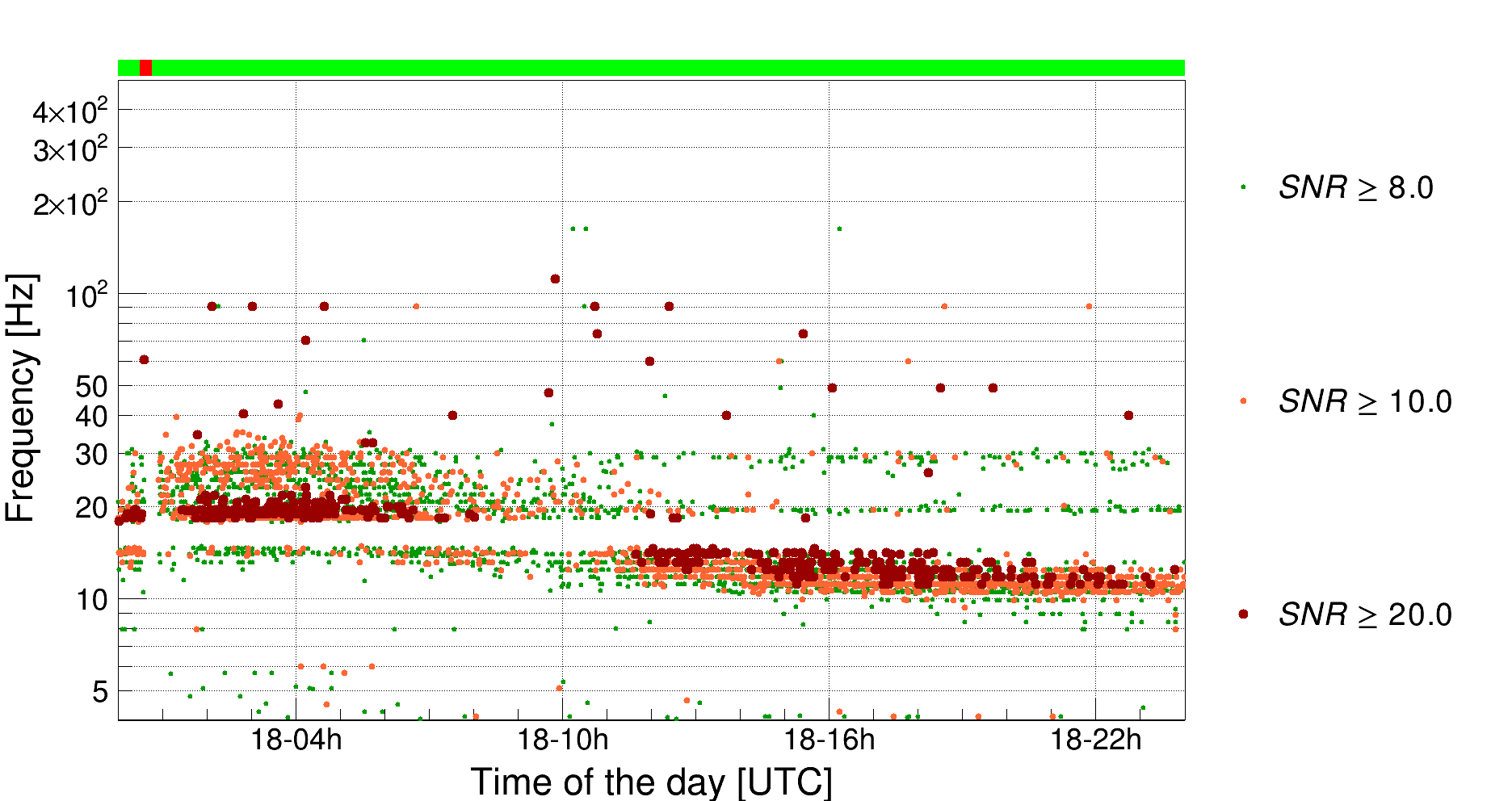
Figure 1: Daily Omicron triggers of DARM for the 18 January 2020. Two clusters of glitches with a high SNR, identified by the larger dots in orange and red, can be observed, one having higher frequency before 11:00UTC and one having lower frequency after 11:00UTC. The difference in frequency of the clusters is consistent with a decrease of the microseismic noise measured at the West end building during the day and reported in Figure 2, the scattered light glitches frequency being proportional to the ground motion amplitude.

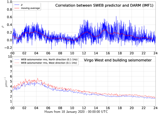
Figure 2: Top: correlation values $\rho$ between the predictor $f_{arch}(t)$ for BENCH-MIRROR and the instantaneous amplitude of DARM’s first oscillatory mode, as extracted by pytvfemd. Bottom: microseismic noise as measured at the Virgo West end building.

3 Results

This section presents the results of the daily analysis. In total 1440 intervals of 60s of data were analysed for each day. As the winter period is typically characterised by higher sea activity and microseismic noise, the following days of the last part of O3b, were chosen:

• 18 January 2020

• 1-2, 9-10, 29 February 2020

• 1-2 March 2020

For these days in O3b, a larger number of low frequency triggers were observed in the Omicron trigger data. Figure 1 shows the daily Omicron triggers of DARM DoF of Virgo during 18 January 2020. Two distinct clusters of scattered light glitches with a high SNR>20 can be seen. The first cluster has frequencies centered around $20$ Hz, and lasts from 00:00 UTC to approximately 11:00 UTC. The second cluster has frequencies centered around $15$ Hz and it lasts until the end of the day. Figure 2 shows the correlation $\rho$ between the BENCH-MIRROR predictor $f_{arch}(t)$ and the $IA(t)$ of DARM’s IMF1, as extracted by pytvfemd. For the 18 of January, a low-pass frequency of $f=20$ Hz was used for the 00:00-11:00 UTC interval while $f=~{}10$ Hz was used from 11:00UTC to the end of the day. This combination of values was found to give the best results i.e., higher values of $\rho$. It can be seen that the $\rho$ values obtained are consistent with the times of occurrence of high SNR glitches in Figure 1, in the UTC time intervals 01:00 - 07:00, 11:00 - 14:00, and 14:00 - 23:00. The moving average of $\rho$ with a window of 60 points, hence one hour, shown in red highlights this.

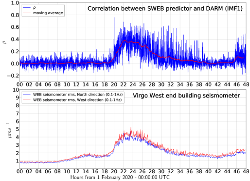
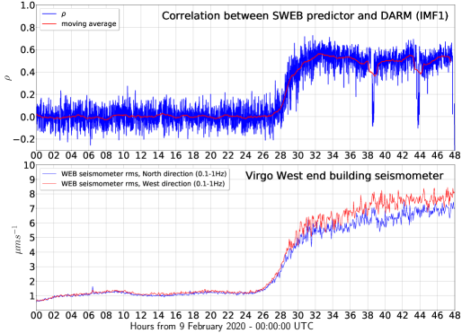
Figure 3: Correlation values between the predictor $f_{arch}(t)$ for BENCH-MIRROR and the IA(t) of DARM’s IMF1, obtained for the 1-2 February period (top) and the 9-10 February (bottom). Also shown, time evolution of the root means square of the West end building seismometer data in the $0.1-1$ Hz frequency band.

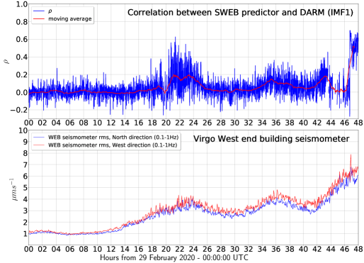
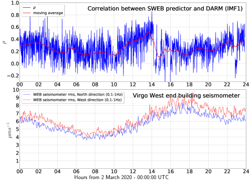
Figure 4: Correlation values between the predictor $f_{arch}(t)$ for BENCH-MIRROR and the IA(t) of DARM’s IMF1, obtained for the 29 February 1 March period (top) and the 2 March (bottom). Also shown, time evolution of the root means square of the West end building seismometer data in the $0.1-1$ Hz frequency band.

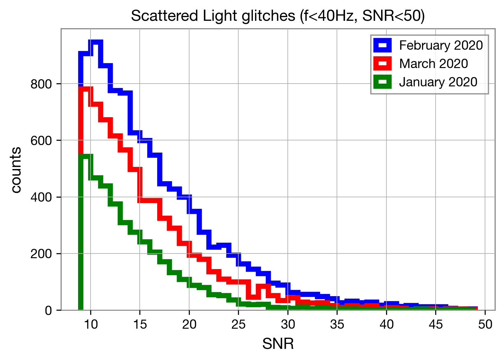
Figure 5: Histogram of SNR of Virgo scattered light glitches, with peak frequency $f<40$ Hz and $SNR<50$, during the first three months of 2020. February has the highest number of glitches, followed by March and January.

Figure 2, bottom panel, shows the time evolution of seismic noise in the microseismic frequency region $0.1-1$ Hz at the Virgo West end building on the 18 January. Higher values at the beginning of the day are observed, related to the higher frequency scattered light glitches. The decrease of microseismic noise is consistent with the observed lower frequency of the second cluster of glitches of Figure 1. Figure 3 shows the $\rho$ values obtained for February 1-2 and February 9-10. A higher correlation, indicative of scattered light noise in the data, is visible in the middle region of the plot. Also shown is the seismometer data, which are highly correlated with the $\rho$ time series of the top panel. Figure 4 reports the $\rho$ values obtained for the 29 February - 2 March period, along with seismometer data. Sudden drops in the values of $\rho$, are obtained from data following lock loss of the detector i.e., when not all the optical cavities are resonant, and correspond to periods in which the full lock is not yet achieved. More details on the lock acquisition procedure are in [28]. Figure 2, 3 and 4 show that an increase of microseismic noise leads to an increase in scattered light noise witnessed in DARM due to the West end bench i.e., high correlation values between the SWEB predictor and the instantaneous amplitude of DARM’s IMF1. Regarding the 2 March, an increase in seismic noise in the $0.03-0.1$ Hz is also measured by the seismometer in the West end building (not shown), coincident with the increase of $\rho$ in the middle part of the plot. To further investigate the relationship between scattered light glitches and microseismicity, Figure 5 shows histograms of the signal-to-noise ratio (SNR) of Virgo glitches classified as scattered light by GravitySpy [29] with $SNR<50$ during January, February and March 2020. Scattered light glitches with peak frequency $f<40$ Hz and for which the duration is shorter than their separation in time were considered. It can be seen that February has the highest number of glitches, followed by March and January. Changes in the amounts of scattered light glitches are possibly due to different levels of microseismicity during the considered months.

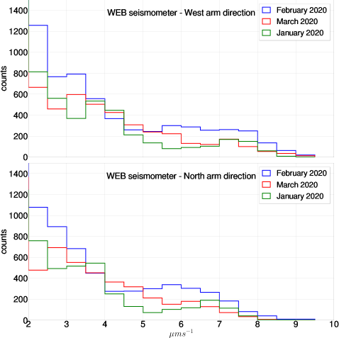
Figure 6: Histogram of Virgo West end building seismometer data in the microseismic frequency region, horizontal components. Only velocities greater than $v=2$$\mu\mathrm{m}\mathrm{s}^{-1}$ are shown. Velocities greater than $v=5$$\mu\mathrm{m}\mathrm{s}^{-1}$ are more frequent in February, wrt March and January 2020.

To verify this, Figure 6 reports histograms of the West end building seismometer data, horizontal components, in the microseismic band i.e., $0.1-1$ Hz, for the same period. Velocities greater than $v=5$$\mu\mathrm{m}\mathrm{s}^{-1}$ are more frequent in February followed by March and January 2020, as expected.

4 Conclusions

The pytvfemd adaptive algorithm was applied to the DARM DoF of the Virgo detector to extract the oscillatory mode related to scattered light noise, from which its instantaneous amplitude IA(t) can be obtained. The IA(t) time series is known to correlate with the predictor computed from the velocity of the optic generating scattered light. Daily analysis were carried out, using the relative motion of the West end bench wrt the West end mirror to obtain the predictor from Equation 1. The analysis obtains a total of 1440 values of Pearson correlation coefficients $\rho$ each day. The time evolution of $\rho$ values is consistent with the clusters of scattered light glitches in the Omicron triggers plot of 18 January, shown in Figure 1. Omicron triggers for the other days considered are in Appendix B. Furthermore, the obtained values of $\rho$ are found to be correlated with seismometer data in the microseismic frequency band. The data considered are from the winter period, during which higher microseismic noise is expected. This excess of low frequency noise can couple to the detector in the form of scattered light as it possibly affects the suspended optical benches. Obtained results indicate that the adopted methodology, based on the pytvfemd adaptive algorithm, is suitable to monitor the onset and evolution of scattered light noise, related to environmental noise variability in GW interferometers. As the source of scattered light during O3 was known to be the West end bench, this noise was mainly removed during the online noise subtraction using the relevant photodiode as a witness channel [30]. This allowed to remove the scattered light noise so that it would not significantly affect the gravitational wave strain data. The issue concerning the West end bench control was identified and cured after O3, and its residual motion is expected to be similar to the one of the other terminal bench, located at the end of the North Arm of the detector. To make the adopted methodology automated, the expected peak frequency of the scattered light glitches could be used as low-pass frequency cutoff. One daily analysis takes approximately 1.5 hours on Condor [31]. This allows to foresee a daily monitoring of possible scattered light culprits during the pre-O4 noise hunting phase and then during the run itself.

Appendix A: Scattered light arches in DARM spectrogram

The distinctive feature of scattered light noise in the data is the presence of arches appearing in their spectrogram. Equation 1 is indicative of the frequency and time of occurrence of such arches. Hence, if the source of scattered light has been correctly identified, the predictor overlaps with the arches in the spectrogram. Figure A1 shows the spectrogram of DARM and the predictor for the West end bench for the 1 February 2020, as obtained for one minute of data. The starting time is 20:01:00 UTC. It can be seen that the predictor overlaps with the arches, confirming that the West end bench is the culprit of the observed scattered light noise.

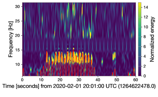
Figure A1: Shown in red is the predictor $f_{arch}(t)$ computed for the West End Bench and overlapped on the spectrogram of the DARM DoF of the detector. The scattered light arches are visible in yellow, having frequency up to $15$ Hz.

Appendix B: Daily Omicron plots

Shown are the Omicron daily triggers of Virgo DARM DoF for the days considered in this study. The onset and time evolution of low frequency glitches is visible. The colour scale indicate the signal-to-noise ratio (SNR) of the glitches. The green and red bar on top indicates periods in which the detector is locked or unlocked, respectively.

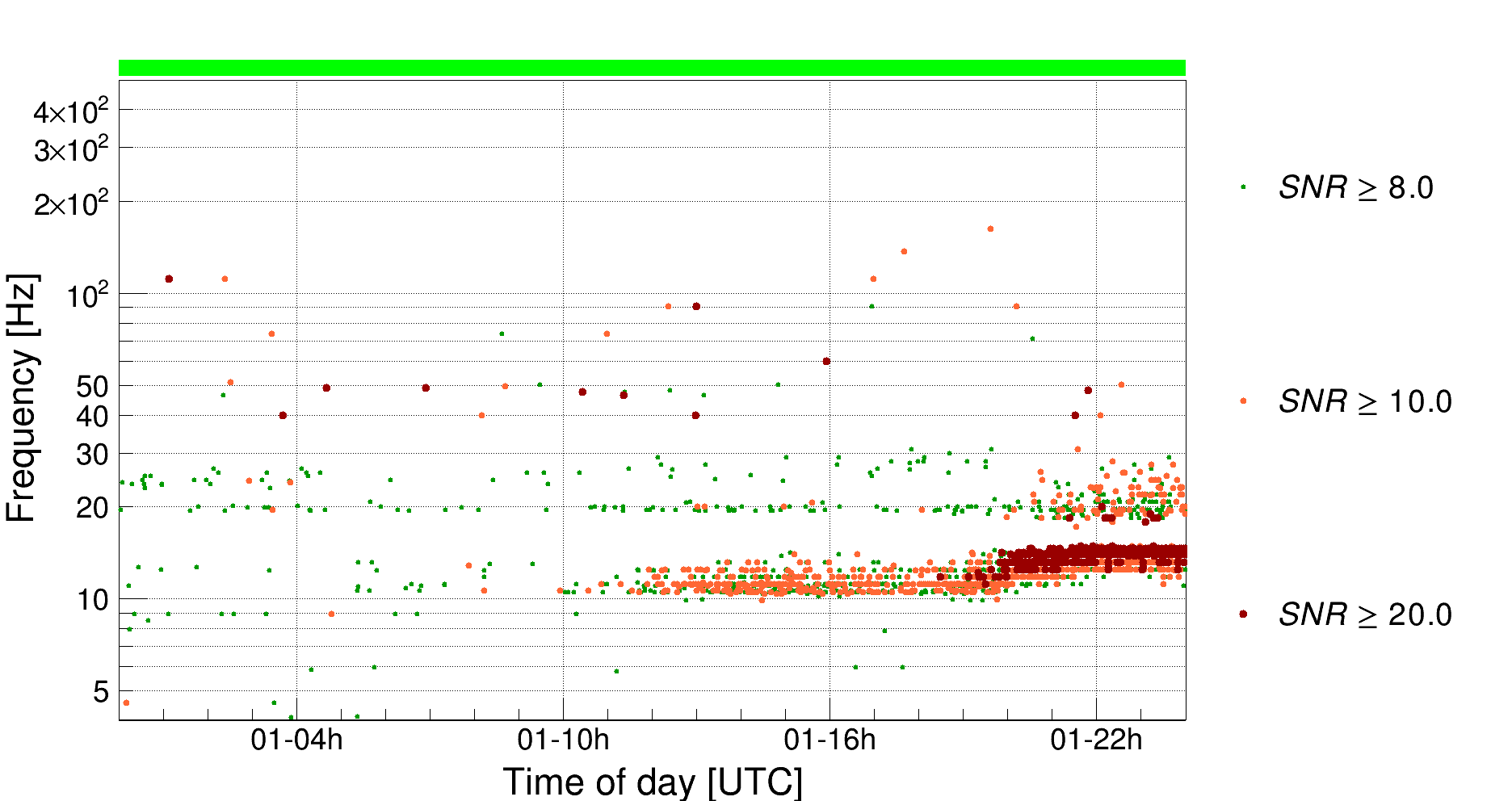
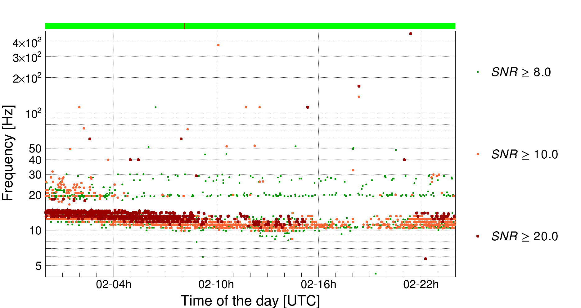
Figure B1: The daily Omicron plots for the 1 of February 2020 (top) and for the 2 of February 2020 (bottom) are shown.

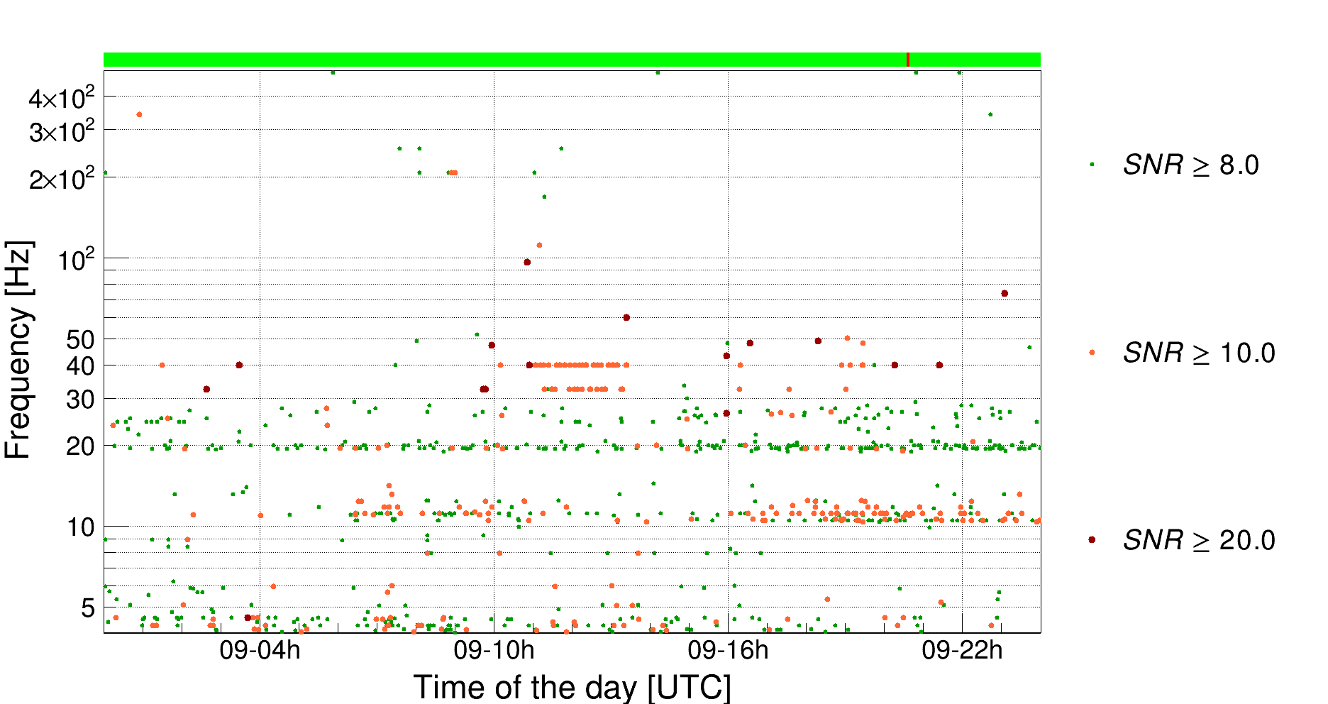
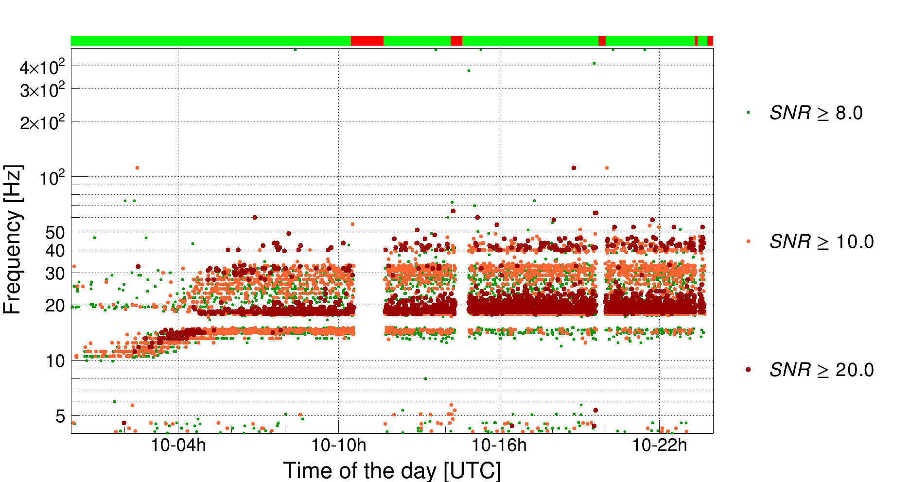
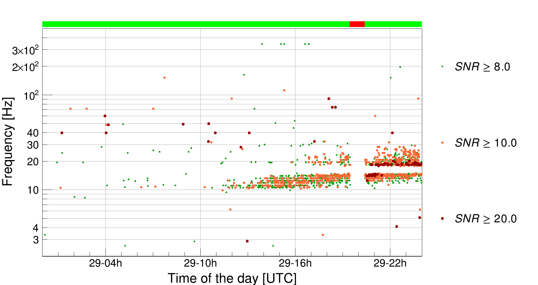
Figure B2: From top to bottom, reported here are the daily Omicron plots for the 9, 10 and 29 February 2020.

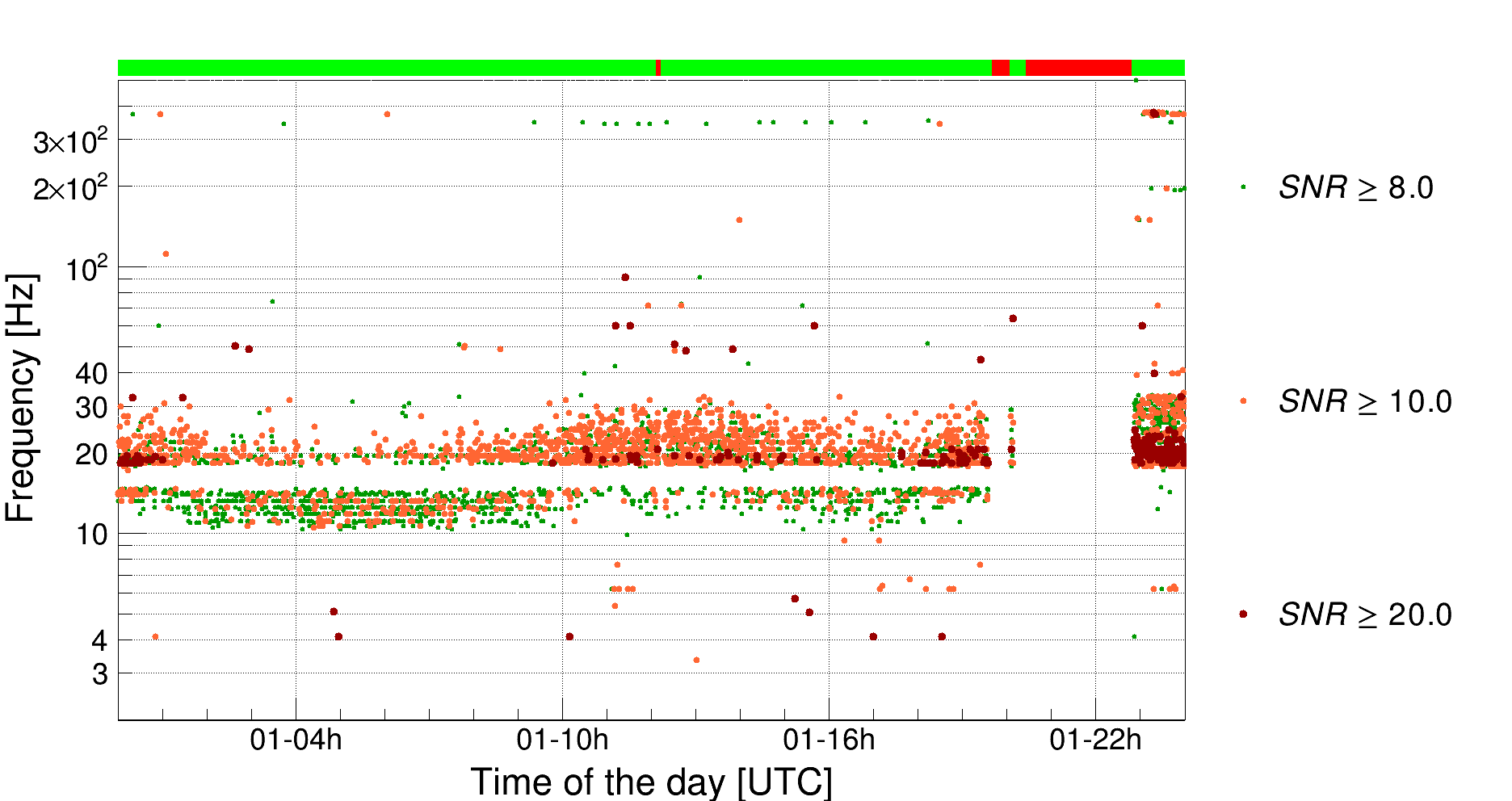
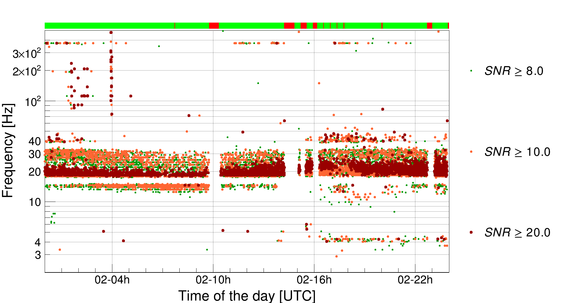
Figure B3: Daily Omicron plots for the 1 (top) and 2 (bottom) of March 2020 are shown.

References

- [1] F. Acernese, P. Amico, M. Alshourbagy, F. Antonucci, S. Aoudia, S. Avino, D. Babusci, G. Ballardin, F. Barone, L. Barsotti, et al., “The Virgo status,” Classical and Quantum Gravity, vol. 23, no. 19, p. S635, 2006.
- [2] F. Acernese et al., “Advanced Virgo: a second-generation interferometric gravitational wave detector,” Class. Quant. Grav., vol. 32, no. 2, p. 024001, 2015.
- [3] F. Acernese, P. Amico, M. Alshourbagy, S. Aoudia, S. Avino, D. Babusci, G. Ballardin, F. Barone, L. Barsotti, M. Barsuglia, et al., “Environmental noise studies in Virgo,” in Journal of Physics: Conference Series, vol. 32, p. 013, IOP Publishing, 2006.
- [4] G. Saccorotti, D. Piccinini, L. Cauchie, and I. Fiori, “Seismic noise by wind farms: a case study from the Virgo Gravitational Wave Observatory, Italy,” Bulletin of the Seismological Society of America, vol. 101, no. 2, pp. 568–578, 2011.
- [5] F. Acernese, P. Amico, N. Arnaud, D. Babusci, R. Barillé, F. Barone, L. Barsotti, M. Barsuglia, F. Beauville, M. Bizouard, et al., “Properties of seismic noise at the Virgo site,” Classical and Quantum Gravity, vol. 21, no. 5, p. S433, 2004.
- [6] A. Effler, R. Schofield, V. Frolov, G. González, K. Kawabe, J. Smith, J. Birch, and R. McCarthy, “Environmental influences on the LIGO gravitational wave detectors during the 6th science run,” Classical and Quantum Gravity, vol. 32, no. 3, p. 035017, 2015.
- [7] E. J. Daw, J. A. Giaime, D. Lormand, M. Lubinski, and J. Zweizig, “Long term study of the seismic environment at LIGO,” Class. Quant. Grav., vol. 21, pp. 2255–2273, 2004.
- [8] M. S. Longuet-Higgins, “A theory of the origin of microseisms,” Philosophical Transactions of the Royal Society of London. Series A, Mathematical and Physical Sciences, vol. 243, no. 857, pp. 1–35, 1950.
- [9] R. K. Cessaro, “Sources of primary and secondary microseisms,” Bulletin of the Seismological Society of America, vol. 84, no. 1, pp. 142–148, 1994.
- [10] L. Naticchioni, M. Perciballi, F. Ricci, E. Coccia, V. Malvezzi, F. Acernese, F. Barone, G. Giordano, R. Romano, M. Punturo, et al., “Microseismic studies of an underground site for a new interferometric gravitational wave detector,” Classical and Quantum Gravity, vol. 31, no. 10, p. 105016, 2014.
- [11] A. Gorbatikov, M. Y. Stepanova, and G. Korablev, “Microseismic field affected by local geological heterogeneities and microseismic sounding of the medium,” Izvestiya, Physics of the Solid Earth, vol. 44, no. 7, pp. 577–592, 2008.
- [12] P. D. Bromirski and F. K. Duennebier, “The near-coastal microseism spectrum: Spatial and temporal wave climate relationships,” Journal of Geophysical Research: Solid Earth, vol. 107, no. B8, pp. ESE–5, 2002.
- [13] T. Accadia, F. Acernese, F. Antonucci, P. Astone, G. Ballardin, F. Barone, M. Barsuglia, T. S. Bauer, M. Beker, A. Belletoile, et al., “Noise from scattered light in Virgo’s second science run data,” Classical and Quantum Gravity, vol. 27, no. 19, p. 194011, 2010.
- [14] S. Soni, C. Austin, A. Effler, R. Schofield, G. González, V. Frolov, J. Driggers, A. Pele, A. Urban, G. Valdes, et al., “Reducing scattered light in LIGO’s third observing run,” Classical and Quantum Gravity, vol. 38, no. 2, p. 025016, 2020.
- [15] M. Wąs, R. Gouaty, and R. Bonnand, “End benches scattered light modelling and subtraction in advanced Virgo,” Classical and Quantum Gravity, vol. 38, no. 7, p. 075020, 2021.
- [16] N. Huang, Z. Shen, S. Long, M. Wu, H. Shih, Q. Zheng, and H. Liu, “The empirical mode decomposition and the Hilbert spectrum for nonlinear and non-stationary time series analysis,” Proceedings of the Royal Society of London A: mathematical, physical and engineering sciences, vol. 454, no. 1971, pp. 903–995, 1998.
- [17] N. E. Huang, Hilbert-Huang transform and its applications, vol. 16. World Scientific, 2014.
- [18] Z. Wu and N. Huang, “A study of the characteristics of white noise using the empirical mode decomposition method,” Proceedings of the Royal Society of London A: Mathematical, Physical and Engineering Sciences, vol. 460, no. 2046, pp. 1597–1611, 2004.
- [19] H. Li, Z. Li, and W. Mo, “A time varying filter approach for empirical mode decomposition,” Signal Processing, vol. 138, pp. 146–158, 2017.
- [20] G. Valdes, B. O’Reilly, and M. Diaz, “A Hilbert-Huang transform method for scattering identification in LIGO,” Classical and Quantum Gravity, vol. 34, no. 23, p. 235009, 2017.
- [21] A. Longo, S. Bianchi, W. Plastino, N. Arnaud, A. Chiummo, I. Fiori, B. Swinkels, and M. Was, “Scattered light noise characterisation at the Virgo interferometer with tvf-EMD adaptive algorithm,” Classical and Quantum Gravity, vol. 37, p. 145011, 2020.
- [22] S. Bianchi, A. Longo, G. Valdes, G. González, and W. Plastino, “gwadaptive_scattering: an automated pipeline for scattered light noise characterization,” arXiv:2107.07565v1 [astro-ph.IM], 7 2021.
- [23] S. Bianchi, “stfbnc/pytvfemd v0.1,” Zenodo, February 2021. https://doi.org/10.5281/zenodo.4568706.
- [24] M. Unser, “Splines: A perfect fit for signal and image processing,” IEEE Signal processing magazine, vol. 16, pp. 22–38, 1999.
- [25] P. J. Loughlin and K. L. Davidson, “Modified Cohen-Lee time-frequency distributions and instantaneous bandwidth of multicomponent signals,” IEEE Transactions on Signal Processing, vol. 49, no. 6, pp. 1153–1165, 2001.
- [26] G. Jones and B. Boashash, “Instantaneous frequency, instantaneous bandwidth and the analysis of multicomponent signals,” in International Conference on Acoustics, Speech, and Signal Processing, pp. 2467–2470, IEEE, 1990.
- [27] F. Robinet, N. Arnaud, N. Leroy, A. Lundgren, D. Macleod, and J. McIver, “Omicron: a tool to characterize transient noise in gravitational-wave detectors,” SoftwareX, p. 100620, 2020.
- [28] A. Allocca, D. Bersanetti, J. Casanueva Diaz, C. De Rossi, M. Mantovani, A. Masserot, L. Rolland, P. Ruggi, B. Swinkels, E. N. Tapia San Martin, et al., “Interferometer Sensing and Control for the Advanced Virgo Experiment in the O3 Scientific Run,” Galaxies, vol. 8, no. 4, p. 85, 2020.
- [29] M. Zevin, S. Coughlin, S. Bahaadini, E. Besler, N. Rohani, S. Allen, M. Cabero, K. Crowston, A. K. Katsaggelos, S. L. Larson, et al., “Gravity Spy: integrating advanced LIGO detector characterization, machine learning, and citizen science,” Classical and quantum gravity, vol. 34, no. 6, p. 064003, 2017.
- [30] F. Acernese et al., “Calibration of Advanced Virgo and reconstruction of detector strain h(t) during the Observing Run O3,” arXiv:2107.03294 [gr-qc], 7 2021.
- [31] B. Bockelman, T. Cartwright, J. Frey, E. Fajardo, B. Lin, M. Selmeci, T. Tannenbaum, and M. Zvada, “Commissioning the htcondor-ce for the open science grid,” in Journal of Physics: Conference Series, vol. 664, p. 062003, IOP Publishing, 2015.