Nekhoroshev estimates
for the orbital stability of Earth’s satellites

Abstract.

We provide stability estimates, obtained by implementing the Nekhoroshev theorem, in reference to the orbital motion of a small body (satellite or space debris) around the Earth. We consider a Hamiltonian model, averaged over fast angles, including the $J_{2}$ geopotential term as well as third-body perturbations due to Sun and Moon. We discuss how to bring the Hamiltonian into a form suitable for the implementation of the Nekhoroshev theorem in the version given by [Pös93] for the ‘non-resonant’ regime. The manipulation of the Hamiltonian includes i) averaging over fast angles, ii) a suitable expansion around reference values for the orbit’s eccentricity and inclination, and iii) a preliminary normalization allowing to eliminate particular terms whose existence is due to the non-zero inclination of the invariant plane of secular motions known as the ‘Laplace plane’. After bringing the Hamiltonian to a suitable form, we examine the domain of applicability of the theorem in the action space, translating the result in the space of physical elements. We find that the necessary conditions for the theorem to hold are fulfilled in some non-zero measure domains in the eccentricity and inclination plane $(e,i)$ for a body’s orbital altitude (semi-major axis) up to about 20 000 km. For altitudes around 11 000 km we obtain stability times of the order of several thousands of years in domains covering nearly all eccentricities and inclinations of interest in applications of the satellite problem, except for narrow zones around some so-called ‘inclination-dependent’ resonances. On the other hand, the domains of Nekhoroshev stability recovered by the present method shrink in size as the semi-major axis $a$ increases (and the corresponding Nekhoroshev times reduce to hundreds of years), while the stability domains practically all vanish for $a>20000$ km.

1. Introduction

The study of the stability of the motion of celestial bodies is relevant from both the theoretical and practical points of view; such investigation can be approached using numerical or analytical tools (see [Cel10]) for a review). In this work, we consider the problem of the long-term (over $10^{3}-10^{4}$ years) stability of a small body (satellite or space debris) in orbit around the Earth and subject to third-body perturbations due to the Moon and the Sun. By stability we mean that the body undergoes no large variations of its orbital elements that could produce a drastic change (e.g., escape) in the orbit.

In the orbital study of satellite motions, it is convenient to split the space environment around the Earth into three distinct regions according to the distance from the Earth’s surface, where different elements can affect the dynamics:

• LEO: Low-Earth-Orbit (from $90$ to $2\,000$ km of altitude), where the Earth’s atmosphere generates dissipative effects;

• MEO: Medium-Earth-Orbit (between $2\,000$ and $30\,000$ km of altitude) and GEO: Geostationary-Earth-Orbit (altitudes around the geosynchronous orbit at about $35\,786$ km), where the dissipative effect of the atmosphere is negligible and the dynamical system associated with the equations of motion is conservative. In these regimes, the most important contributions are due to the geopotential and to the lunar and solar third-body perturbations.

We will hereafter consider a Hamiltonian model for the motion of small bodies at MEO (see, instead, [CG18, LCG16] for the inclusion of dissipative effects). The study of dynamics at MEO in the conservative regime has been subject of many works, including the development of analytical models (e.g., [CG14, CEG⁺17, Gia74, Kau62, Lan89]), study of resonances (e.g., [Bre01a, Bre01b, CGL20, CGP16, CGPR17, CG04, Coo62, EH97, Hug80, LDV09]), as well as the dynamical chartography (stability maps, onset of chaos) of the MEO region (e.g., [ADR⁺16, CPL15, DRA⁺16, GDGR16, RS13, RARV15, RDT⁺16, Ros08, SRTV19, VL08]).

The aim of this work is to study the stability of a model for objects in MEO from an analytical point of view, providing exponential stability estimates using the celebrated Nekhoroshev theorem ([Nek77]). We stress that, while the Nekhoroshev theorem is particularly relevant for systems with three or more degrees of freedom, which can be affected by the phenomenon known as Arnold diffusion ([Arn64]), the applicability of the theorem in securing the long-term stability in open domains in the action space holds for systems of any number of degrees of freedom larger than or equal to two. Furthermore, the Nekhoroshev theorem was originally developed under a suitable non-degeneracy condition, called steepness, while later approaches (e.g. [BG86, Pös93]) focus on the important subcase of convex and quasi-convex Hamiltonians (see [Pös93] for definitions). As regards the applications, the theorem was proved useful in obtaining realistic estimates of the domains or times of practical stability of the orbits in a number of interesting problems in Celestial Mechanics. Among others, we mention the three-body problem ([CF96]) as well as the problem of the Trojan asteroids ([CG91], [GS97]).

In this work, we apply the Nekhoroshev theorem to a model approximating the (averaged over short period terms) dynamics of a small body around the Earth. As discussed below, this allows to obtain long-time stability estimates for realistic sets of parameters, at least for altitudes (values of the semi major axis) below 20 000 km.

We consider a model ruled by a Hamiltonian function obtained as the sum of different contributions, namely, the geopotential $J_{2}$ term as well as the third-body perturbations on the small body by the Sun and Moon. Several studies (see [DRA⁺16, GDGR16, AHA21, NG21] and references therein) have demonstrated the relevance of this model in capturing all important effects for the long-term dynamics at MEO.

An important aspect of our present work concerns a number of preliminary operations performed on the initial Hamiltonian, which turn to be crucial to the purpose of bringing the Hamiltonian in a form allowing to explicitly demonstrate the fulfilment of the conditions for the holding of the Nekhoroshev theorem in the form given in [Pös93]. These preliminary steps are explained in detail in Section 2 below, and can be summarized as follows:

(i) Average over fast angles. We start by averaging the Hamiltonian over the problem’s fast angles, i.e., the mean anomalies of the small body’s, Moon’s and Sun’s orbits. After this operation, the semi-major axis $a$ of any orbit becomes a constant which can be used to label the altitude of each orbit.

(ii) Expansion around reference values in the eccentricity and inclination. The remaining elements (eccentricity $e$ and inclination $i$), which can be mapped into the action variables of the problem, undergo ‘secular’ (slow) evolution under the averaged Hamiltonian. Our purpose is to characterize the stability of the orbits in the space $(e,i)$ of the orbital elements. To this end, fixing a grid of reference values $(e_{*},i_{*})$ in the plane $(e,i)$ for each (constant) semi-major axis $a=a_{*}$, we perform a Taylor expansion of the averaged Hamiltonian around the points in action space associated with the reference point $(e_{*},i_{*})$. This step is important, since the Taylor-expanded Hamiltonian can be easily manipulated in terms of normalizing canonical transformations necessary to perform with the aid of a computer-algebraic program (see below).

(iii) Preliminary normalization. We perform a preliminary normalization of the averaged and Taylor-expanded Hamiltonian, aiming to eliminate some terms which, albeit reflecting a trivial dynamics (see Section 3), may artificially affect the estimates found by implementing Pöschel’s version of the Nekhoroshev theorem. We argue below that this step is a consequence of the non-zero value of the inclination of the Laplace plane with respect to the Earth’s equatorial plane. The inclination can be expressed as

$$i^{(p)}\simeq-\frac{A}{2B}\frac{1}{(\mu_{E}a)^{1/4}}\ ,$$ (1)

where

$$\begin{split}&A=-\frac{3R_{E}^{2}a^{7/4}\sin{(2i_{0})}}{8(\mu_{E})^{1/4}}\left(\frac{\mu_{M}}{a_{M}^{3}}+\frac{\mu_{\odot}}{a_{\odot}^{3}}\right),\\ &B=\frac{3}{4}\frac{\sqrt{\mu_{E}}R_{E}^{2}J_{2}}{a^{7/2}}+\frac{3\mu_{M}(2-3\sin^{2}{i_{0}})}{16\sqrt{\frac{\mu_{E}}{a^{3}}}a_{M}^{3}}+\frac{3\mu_{\odot}(2-3\sin^{2}{i_{0}})}{16\sqrt{\frac{\mu_{E}}{a^{3}}}a_{S}^{3}}\end{split}$$ (2)

with $R_{E},\mu_{E}$ being the Earth’s mean radius and mass parameter, $a_{M},\mu_{M}$ are the Moon’s semimajor axis and mass parameter, $a_{\odot},\mu_{\odot}$ are the Sun’s semimajor axis and mass parameter, and finally $i_{0}$ is the inclination of the ecliptic plane. A key result in the present paper is the use of normal form techniques to reduce the size, in the Hamiltonian, of all terms related to the Laplace plane (see Section 3); whenever convergent, this procedure is crucial to put the initial Hamiltonian in a form for which Nekhoroshev’s nonresonant stability estimates can be produced, since it allows us to control the norm of the perturbing function under a suitable choice of the domain in the actions.

$\alpha$	$\beta$	$i(deg)$	$\alpha$	$\beta$	$i(deg)$	$\alpha$	$\beta$	$i(deg)$	$\alpha$	$\beta$	$i(deg)$
1	0	63.43	0	1	90	1	1	46.37	1	-1	73.1
2	1	56	1	2	0	2	-1	69	-1	12	78
3	1	58.75	3	-1	67.33	1	-3	81.47

Table 1. Inclination-dependent resonances of order $\leq 4$ in the lunisolar model. The coefficients are such that $\alpha\dot{\omega}+\beta\dot{\Omega}=0$, where $\omega$ is the argument of the perigee and $\Omega$ is the longitude of the ascending node ([Hug80]).

Now, following steps (i) to (iii) above, the procedure leads to a normalized 2-dimensional Hamiltonian expressed in suitably defined action-angle variables $(\mathbf{I},\mathbf{u})\in{\mathbb{R}}^{2}\times{\mathbb{T}}^{2}$, of the form:

$$\mathcal{H}(\mathbf{I},\mathbf{u})=h_{0}(\mathbf{I})+h_{1}(\mathbf{I},\mathbf{u})\ .$$ (3)

Using the Hamiltonian (3), we can derive stability results on the eccentricity and the inclination by implementing the estimates provided in Proposition 1 of [Pös93]. This proposition refers to the so-called non-resonant regime, i.e., when the fundamental frequencies deduced by the integrable part of the Hamiltonian, $h_{0}$, are subject to no resonance conditions. Under particular assumptions on the non-resonance condition for $h_{0}$, as well as on the smallness of the norm of $h_{1}$ in a suitable functional space and domain in the action variables (see Section 3.1), one can prove that the actions remain in a small neighborhood of their initial values for a period of time which is exponentially long with respect to the norm of $h_{1}$. We remark that Proposition 1 in [Pös93] does not require any convexity assumption on the Hamiltonian. This assumption is relevant when analyzing resonant regimes (for a thorough analysis of different non-degeneracy conditions such as convexity, quasi-convexity, 3-jet, etc., see [DBCE21]). However, we also stress that, despite our use of Pöschel’s proposition in the non-resonant regime, the presence of resonances at MEO plays an important role also in our results, as becomes evident in the discussion of our results in Section 4. In fact, we find that our obtained stability domains typically exclude some zones around the so-called inclination-dependent resonances ([Hug80]), i.e., resonances appearing for particular values of the inclination of the orbit, independently of the value of the semimajor axis or the eccentricity. This is because the series constructed in our preliminary normalization of the Hamiltonian are affected by small divisors related to the most-important of these resonances, given in Table 1. Also, the frequencies associated with these divisors influence the determination of the so-called ‘Fourier cut-off’ (Section 3) which appears in the implementation of the Proposition 1 of [Pös93].

As described in Section 4, the stability estimates obtained in this work strongly depend on the distance of the small body from the Earth’s center: our results show that the domain of Nekhoroshev stability in the plane $(e,i)$ has a large volume (limited only by narrow strips around resonances) at the distance of 10 000 km, while it shrinks to a near-zero volume beyond the distance of 20 000 km. We should stress that this result is partly due to the dynamics itself (the $J_{2}$ dynamics alone is integrable, but the third body perturbations increase in relative size as the distance from the Earth increases), but also probably due, in part, to our particular technique used to apply the Nekhoroshev theorem, i.e. including the processing of the Hamiltonian as described in steps (i)-(iii) above. We thus leave open the possibility that this latter constraint be relaxed with the use of a better technique. Also, our present treatment is simplified in that we ignore the periodic oscillation of the Moon’s line of nodes (by an amplitude of $~{}11.5^{\circ}$ over a period of $18.6$ yr) and inclination (by $\pm 5^{\circ}$) around the ecliptic of the Moon’s orbit with respect to the Earth’s equatorial plane. This oscillation introduces one more secular frequency to the problem; however, it substantially affects the orbits only for semi-major axes $a>20\,000$ km, which is, anyway, beyond the domain of stability presently found even while ignoring this effect.

As a final remark, in [DBCE21] we studied the satellite’s stability in two different models: the $J_{2}$ approximation of the geopotential and a model that includes $J_{2}$, Sun and Moon. We computed suitable normal forms and obtained stability results by estimating the size of the remainder function after the normalizing transformation. In [DBCE21] we only considered values of the eccentricity and inclination close to zero and to the inclination of the Laplace plane, respectively; besides, our stability estimates were not obtained separately for eccentricity and inclination, but only as regards their combination $\sqrt{1-e^{2}}\cos{i}$ through the Lidov-Kozai integral. This is a main difference with respect to the present paper, in which we consider generic values for the eccentricity and inclination.

This article is organized as follows: Section 2 provides the construction of the secular Hamiltonian function which describes the model, as well as its normalization; in Section 3 the theoretical framework is described, along with the algorithm used to produce the normalized Hamiltonian and the stability estimates; Section 4 describes the results.

2. Hamiltonian preparation

In this Section, we provide details on the model (Section 2.1), on the corresponding secular Hamiltonian function averaged over fast angles (Section 2.2), the expansion around some reference values for the eccentricity and inclination (Section 2.3), and the preliminary normalization to remove specific terms (Section 2.4).

2.1. Model

We consider a small body (satellite or debris) $S$ of infinitesimal mass, under the action of the Earth’s gravitational field and the third-body perturbations due to the Moon and Sun. Geocentric inertial Cartesian coordinates are denoted by $(x,y,z)$, where the $xy$-plane coincides with the Earth’s equatorial plane, $z$ points to the north pole, and $x$ points to a fixed direction (ascending node of the Sun’s geocentric orbit). We denote by $\mathbf{r}(t)=(x(t),y(t),z(t))$ the time-evolving radius vector of the body $S$, and by $(a,e,i,M,\omega,\Omega)$ the osculating orbital elements of $S$, where $a$ is the semimajor axis, $e$ the eccentricity, $i$ the inclination with respect to the Earth’s equatorial plane, $M$ is the mean anomaly, $\omega$ the argument of the perigee and $\Omega$ the longitude of the ascending node.

In the sequel, we consider the following approximation to the body’s equations of motion:

$$\ddot{\mathbf{r}}=-\nabla V_{E}(\mathbf{r})-\mu_{\odot}\bigg{(}\frac{\mathbf{r}-\mathbf{r}_{\odot}}{|\mathbf{r}-\mathbf{r}_{\odot}|^{3}}+\frac{\mathbf{r}_{\odot}}{|\mathbf{r}_{\odot}|^{3}}\bigg{)}-\mu_{M}\bigg{(}\frac{\mathbf{r}-\mathbf{r}_{M}}{|\mathbf{r}-\mathbf{r}_{M}|^{3}}+\frac{\mathbf{r}_{M}}{|\mathbf{r}_{M}|^{3}}\bigg{)}\ ,$$ (4)

where $V_{E}(\mathbf{r})$ approximates the geopotential via the relation

$$V_{E}(\mathbf{r})=V_{kep}(|\mathbf{r}|)+V_{J_{2}}(\mathbf{r})\ ,$$ (5)

where $V_{kep}(r)=-{\mu_{E}\over r}$ and $V_{J_{2}}$ in spherical co-ordinates $(r,\varphi,\phi)$ is given by

$$V_{J_{2}}(r,\varphi,\phi)=\frac{\mu_{E}J_{2}}{r}\left\{\left(\frac{R_{E}}{r}\right)^{2}\left(\frac{3}{2}\sin^{2}{\phi}-\frac{1}{2}\right)\right\}.$$ (6)

In the above formulas:

• $\mathcal{G}$ is the gravitational constant, $\mu_{E}=\mathcal{G}m_{E}$, $\mu_{M}=\mathcal{G}m_{M}$, $\mu_{\odot}=\mathcal{G}m_{\odot}$ with $m_{E}$, $m_{M}$, $m_{\odot}$ the masses of the Earth, Moon and Sun respectively.

• We adopt the value $J_{2}=1.082\times 10^{-3}$ for the $J_{2}$ coefficient, and $R_{E}=6\,400$ km for the Earth’s equatorial radius.

• $\mathbf{r}$, $\mathbf{r}_{\odot}$ and $\mathbf{r}_{M}$ are, respectively, the geocentric position vectors of $S$, Sun and Moon.

The expressions of $\mathbf{r}_{\odot}$ and $\mathbf{r}_{M}$ depend on the assumptions on the orbits of Sun and Moon. In this work, the geocentric orbit of the Sun is taken as a fixed ellipse with $a_{\odot}=1.496\times 10^{8}$ km, $e_{\odot}=0.0167$ and $i_{\odot}=23.44^{\circ}$, while the geocentric orbit of the Moon is taken as a fixed ellipse with orbital parameters $a_{M}=384\,748$ km, $e_{M}=0.0554$ and $i_{M}=i_{\odot}$. The last assumption has an important effect on the dynamics: it implies that the only lunisolar resonances which affect the dynamics of the body are those whose location in the element space $(a,e,i)$ depends only on the inclination (see [Hug80]). More resonances, instead, appear when the effect of nodal precession (by a period of 18.6 years) of the Moon’s orbit is taken into account. However, these resonances affect the dynamics only at altitudes exceeding the ones where we presently establish Nekhoroshev stability (see [GDGR16] and Section 4 below), thus they can be ignored in the framework of our present study.

The Hamiltonian function which describes the motion of $S$ can be expressed as the sum of three contributions:

$$\mathcal{H}=\mathcal{H}_{E}+\mathcal{H}_{\odot}+\mathcal{H}_{M},$$ (7)

where $\mathcal{H}_{E}=\mathbf{p}^{2}/2+V_{E}(\mathbf{r})$ with $\mathbf{p}=\mathbf{\dot{r}}$, and $\mathcal{H}_{\odot}$ and $\mathcal{H}_{M}$ are the solar and lunar third-body perturbation terms. Considering the quadrupolar expansion of the third-body perturbation terms in the equations of motion (4), we find

$$\begin{split}\mathcal{H}_{\odot}&=V_{\odot}(\mathbf{r})=-\frac{\mu_{\odot}}{|\mathbf{r}-\mathbf{r_{\odot}}|}+\frac{\mu_{\odot}}{r_{\odot}^{3}}\mathbf{r}\cdot\mathbf{r_{\odot}}\\ &=-\frac{\mu_{\odot}}{r_{\odot}}-\frac{\mu_{\odot}}{2r_{\odot}^{3}}r^{2}+\frac{3}{2}\frac{\mu_{\odot}(\mathbf{r}\cdot\mathbf{r}_{\odot})^{2}}{r_{\odot}^{5}}+O\left(\left(\frac{r}{r_{\odot}}\right)^{3}\right)\ ,\end{split}$$ (8)

$$\begin{split}\mathcal{H}_{M}&=V_{M}(\mathbf{r})=-\frac{\mu_{M}}{|\mathbf{r}-\mathbf{r_{M}}|}+\frac{\mu_{M}}{r_{M}^{3}}\mathbf{r}\cdot\mathbf{r_{M}}\\ &=-\frac{\mu_{M}}{r_{M}}-\frac{\mu_{M}}{2r_{M}^{3}}r^{2}+\frac{3}{2}\frac{\mu_{M}(\mathbf{r}\cdot\mathbf{r}_{M})^{2}}{r_{M}^{5}}+O\left(\left(\frac{r}{r_{M}}\right)^{3}\right)\ .\end{split}$$ (9)

2.2. Average over fast angles - Secular Hamiltonian

The secular motion of the body $S$ can be modeled by computing the average of (7) over all canonical angles associated to the fast motions of $S$, the Sun and the Moon. Note that the period of the Sun is only ‘semi-fast’ (one year, compared to secular periods of $\sim 10$ yrs for the small body), and more detailed models can consider also the case of ‘semi-secular’ resonances, i.e., resonances in the case in which the equations of motion (and Hamiltonian) are not averaged with respect to the Sun’s mean anomaly (see, for example, [CEG⁺17]).

Averaging with respect to all fast angles leads to the following, called hereafter, secular Hamiltonian, given by the sum of the averaged contributions of the Earth, Sun and Moon:

$$\mathcal{H}^{(sec)}=\mathcal{H}_{E}^{(av)}+\mathcal{H}_{\odot}^{(av)}+\mathcal{H}_{M}^{(av)}\ .$$ (10)

The function $\mathcal{H}^{(sec)}=\mathcal{H}^{(sec)}(G,\Theta,\omega,\Omega)$ is a two degrees of freedom Hamiltonian, which can be explicitly computed in terms of Delaunay canonical action-angle variables $G$, $\Theta$ (with conjugated angles $\omega$, $\Omega$), related to the orbital elements by the expressions (see, e.g., [Cel10]):

$$G=\sqrt{\mu_{E}a(1-e^{2})},~{}~{}~{}\Theta=\sqrt{\mu_{E}a(1-e^{2})}\cos i~{}~{}.$$ (11)

Since the averaged Hamiltonian does not depend on the mean anomaly $M$ of $S$, the conjugated Delaunay action $L=\sqrt{\mu_{E}a}$, and hence the semi-major axis $a$, is a constant of motion of the Hamiltonian $\mathcal{H}^{(sec)}$. We set $L=L_{*}$, or, equivalently, $a=a_{*}$ when referring to trajectories whose semi-major axis has the reference value $a_{*}$.

Following a well-known procedure (e.g., [Kau62]), the various terms in the secular Hamiltonian can be computed as follows: for the geopotential term we have

$$\mathcal{H}_{E}^{(av)}=\frac{1}{2\pi}\int_{0}^{2\pi}(\mathcal{H}_{kep}+\mathcal{H}_{J_{2}})dM=\mathcal{H}_{kep}^{(av)}+\mathcal{H}_{J_{2}}^{(av)}\ ,$$

where $\mathcal{H}_{kep}=\mathbf{p}^{2}/2+V_{kep}$, $\mathcal{H}_{J_{2}}=V_{J_{2}}$, which leads to

$$\mathcal{H}_{E}^{(av)}=-\frac{\mu_{E}^{2}}{2L^{2}}-J_{2}\frac{\mu_{E}R_{E}^{2}}{a_{*}^{3}(1-e^{2})^{3/2}}\left(\frac{1}{2}-\frac{3}{4}\sin^{2}{i}\right)\ .$$ (12)

For the terms $\mathcal{H}_{\odot}^{(av)}$, $\mathcal{H}_{M}^{(av)}$ we compute the integral

$$\mathcal{H}_{\odot}^{(av)}={1\over 4\pi^{2}}\int_{0}^{2\pi}\int_{0}^{2\pi}\left(-\frac{\mu_{\odot}}{r_{\odot}}-\frac{\mu_{\odot}}{2r_{\odot}^{3}}r^{2}+\frac{3}{2}\frac{\mu_{\odot}(\mathbf{r}\cdot\mathbf{r}_{\odot})^{2}}{r_{\odot}^{5}}\right)dMdM_{\odot}$$

(and analogously for $\mathcal{H}_{M}^{(av)}$); it is convenient to change the integration variables from $M$ to $u$ (eccentric anomaly of $S$) and from $M_{\odot}$ to $f_{\odot}$ (true anomaly of the Sun). We note that, up to quadrupolar terms, this yields the same result as considering the Moon and Sun in circular, instead of elliptic, orbits (in which case $M_{\odot}$, $M_{M}$ would be equal to $f_{\odot},f_{M}$), but replacing each third-body’s semi-major axis $a_{b}$ with the expression $a_{b}\rightarrow a_{b}(1-e_{b}^{2})^{1/2}$ (index $b$ standing for Sun or Moon). This replacement accomplishes the first step in the Hamiltonian preparation.

2.3. Expansion around reference values $(e_{*},i_{*})$

After performing the above operations, the Hamiltonian $\mathcal{H}^{(sec)}$ becomes a function of the body’s action-angle variables $(G,\omega)$, $(\Theta,\Omega)$, while it depends also on the Delaunay action $L$, which however, does not affect the secular dynamics and can be carried on all subsequent expressions as a parameter (equal to $L_{*}$). We use, alternatively, $a_{*}$ as the parameter appearing in the coefficients of all trigonometric terms in $\mathcal{H}^{(sec)}$. Furthermore, it turns convenient to express $\mathcal{H}^{(sec)}$ in terms of modified Delaunay variables instead of the original Delaunay variables. Let $\delta L=L-L_{*}$ with $L_{*}=\sqrt{\mu_{E}a_{*}}$. We employ the modified Delaunay variables $(\delta L,\Gamma,\tilde{\Theta},\lambda,p,q)$, related to the original Delaunay variables $(L,G,\Theta,M,\omega,\Omega)$ via the latters’ dependence on the Keplerian elements $(a,e,i,M,\omega,\Omega)$. We have

$$\begin{cases}\delta L=L-L_{*}=\sqrt{\mu_{E}a}-\sqrt{\mu_{E}a_{*}}\\ \Gamma=L-G=\sqrt{\mu_{E}a}(1-\sqrt{1-e^{2}})\\ \tilde{\Theta}=G-\Theta=\sqrt{\mu_{E}a}\sqrt{1-e^{2}}(1-\cos{i})\\ \end{cases}\begin{cases}\lambda=M+\omega+\Omega\\ p=-\omega-\Omega\\ q=-\Omega\ .\\ \end{cases}$$ (13)

Starting now from the Hamiltonian $\mathcal{H}^{(sec)}(\Gamma,\tilde{\Theta},p,q)$, our goal will be to examine Nekhoroshev stability in a covering of the action space in terms of local neighborhoods around a grid of reference values corresponding to a grid of element values $(a_{*},e_{*},i_{*})$ (see Section 3.2). This motivates to introduce the variables $P^{\prime}$ and $Q^{\prime}$ defined by

$$\begin{cases}P=\Gamma_{*}-\Gamma,\\ Q=\tilde{\Theta}_{*}-\tilde{\Theta}\ ,\end{cases}$$ (14)

where $\Gamma_{*}$ and $\tilde{\Theta}_{*}$ are the values corresponding to the orbital elements $(e_{*},i_{*})$, and compute the Taylor expansion of $\mathcal{H}^{(sec)}$ in powers of the small quantities $(Q,P)$, truncated at a maximum order $N$ (we set $N=12$). We then arrive at the following truncated secular Hamiltonian model

$$\mathcal{H}^{(sec,N)}(P,Q,p,q)=\sum_{j=1}^{N}g^{(j)}(P,Q,p,q)~{}~{}.$$ (15)

In the model (15) we have

$$g^{(1)}(P,Q)=\omega_{1}P+\omega_{2}Q~{}~{}.$$ (16)

For reasons that will become clear later, for $j\geq 2$ we split each of the functions $g^{(j)}(P,Q,p,q)$ as a sum depending only on the actions and a sum depending also on the angles:

$$g^{(j)}(P,Q,p,q)=\sum_{\begin{subarray}{c}\mathbf{l}\in\mathbb{Z}^{2}\\ |\mathbf{l}|=j\end{subarray}}a^{(j)}_{\mathbf{l}}P^{l_{1}}Q^{l_{2}}+\sum_{\begin{subarray}{c}\mathbf{l},\mathbf{k}\in\mathbb{Z}^{2}\\ |\mathbf{l}|=j-2\end{subarray}}b^{(j)}_{\mathbf{l},\mathbf{k}}P^{l_{1}}Q^{l_{2}}e^{i(k_{1}p+k_{2}q)}~{}.$$ (17)

This last splitting completes the second step in the Hamiltonian preparation. The explicit expressions of the quantities $\omega_{1}$, $\omega_{2}$, $a_{\mathbf{l}}$, $b_{\mathbf{l},\mathbf{k}}$ for $j=2$ are given in Appendix A, in terms of the orbital elements of the satellite, Moon and Sun.

2.4. Preliminary normalization

It was already mentioned in Section 1 that the presence of the averaged lunisolar terms in (15) implies the existence of a secular equilibrium solution of Hamilton’s equation’s of motion under the Hamiltonian $\mathcal{H}^{(sec)}$, corresponding to the values $e=0,i=i^{(p)}$ (see Eq.(1)), where $i^{(p)}$ is called the inclination of the Laplace plane. It is easy to see that the non-zero value of the inclination of the Laplace plane is reflected into the Hamiltonian $\mathcal{H}^{(sec,N)}$ by the presence of purely trigonometric terms, i.e., terms with $|\mathbf{l}|=0$. Such terms yield coefficients which are dominant with respect to the remaining terms in the Hamiltonian expansion. Furthermore, in the splitting of the Hamiltonian as $\mathcal{H}=h_{0}(\mathbf{I})+h_{1}(\mathbf{I},\mathbf{u})$, where $(\mathbf{I},\mathbf{u})$ are action-angle variables, as required for the implementation of the Nekhoroshev theorem (see next section), the above terms generate terms with a dominant coefficient largely affecting the size of the perturbation $h_{1}(\mathbf{I},\mathbf{u})$. In the present subsection, we implement a procedure for controlling the size of the terms (15) of the expansion, so that we obtain a Hamiltonian satisfying the norm bounds required for the implementation of the Nekhoroshev theorem.

More specifically, the aim of the normalization algorithm described below is to remove, up a certain order $N_{norm}$ with respect to the expansion (15), the angle-dependent terms which are constant or linear in the actions: this leads to a Hamiltonian $\mathcal{H}^{(N_{norm})}$, in which the norm of the angle-dependent part decreases at least quadratically with the size of the domain $A_{r_{0}}$ in which local action variables are defined.

The normalization procedure relies on the use of Lie series. In every normalization step, the transformed Hamiltonian is given by

$$\mathcal{H}^{(new)}=\exp^{(N)}(\mathcal{L}_{\mathcal{\chi}})\mathcal{H}^{(old)},$$ (18)

where $\mathcal{L}_{\chi}f=\{f,\mathcal{\chi}\}$ ($\{\cdot,\cdot\}$ denotes the Poisson bracket) and $\exp^{(N)}(\mathcal{L}_{\chi})$ is defined by

$$\exp^{(N)}(\mathcal{L}_{\mathcal{\chi}})f=\sum_{s=0}^{N}\frac{1}{s!}\mathcal{L}_{\mathcal{\chi}}^{s}f\ .$$ (19)

To illustrate the procedure, rename the initial Hamiltonian (15) as $\mathcal{H}^{(0)}$ (where superscripts denote how many normalization steps were performed). Then:

$$\mathcal{H}^{(0)}(P,Q,p,q)=\sum_{j=1}^{N}g^{(j,0)}(P,Q,p,q)\ ,$$ (20)

where

$$g^{(1,0)}(P,Q) = \omega_{1}P+\omega_{2}Q$$

$$g^{(j,0)}(P,Q,p,q) = \sum_{\begin{subarray}{c}\mathbf{l}\in\mathbb{Z}^{2}\\ |\mathbf{l}|=j\end{subarray}}a^{(j,0)}_{\mathbf{l}}P^{l_{1}}Q^{l_{2}}+\sum_{\begin{subarray}{c}\mathbf{l},\mathbf{k}\in\mathbb{Z}^{2}\\ |\mathbf{l}|=j-2\end{subarray}}b^{(j,0)}_{\mathbf{l},\mathbf{k}}P^{l_{1}}Q^{l_{2}}e^{i(k_{1}p+k_{2}q)}\,\quad j\geq 2\ .$$ (21)

The second term of the sum (20) takes the form

$$g^{(2,0)}(P,Q,p,q)=\sum_{\begin{subarray}{c}\mathbf{l}\in\mathbb{Z}^{2}\\ |\mathbf{l}|=2\end{subarray}}a^{(2,0)}_{\mathbf{l}}P^{l_{1}}Q^{l_{2}}+\sum_{\mathbf{k}\in\mathbb{Z}^{2}}b^{(2,0)}_{\boldsymbol{0},\mathbf{k}}e^{i(k_{1}p+k_{2}q)}~{}~{}.$$ (22)

The generating function $\chi^{(1)}$ eliminating the above terms has the form

$$\chi^{(1)}(P,Q,p,q)=\sum_{\mathbf{l},\mathbf{k}\in\mathbb{Z}^{2}}x^{(1)}_{\mathbf{l},\mathbf{k}}P^{l_{1}}Q^{l_{2}}e^{i(k_{1}p+k_{2}q)}\ ,$$ (23)

where the coefficients $x^{(1)}_{\mathbf{l},\mathbf{k}}$ are obtained as the solution of the homological equation

$$\{\omega_{1}P+\omega_{2}Q,\chi^{(1)}\}=-\sum_{\mathbf{k}\in\mathbb{Z}^{2}}b^{(2,0)}_{\boldsymbol{0},\mathbf{k}}e^{i(k_{1}p+k_{2}q)}\ ,$$ (24)

namely

$$\chi^{(1)}(p,q)=-\sum_{\mathbf{k}\in\mathbb{Z}^{2}}\frac{b^{(2,0)}_{\boldsymbol{0},\mathbf{k}}}{i(\omega_{1}k_{1}+\omega_{2}k_{2})}e^{i(k_{1}p+k_{2}q)}\ .$$ (25)

The normalized Hamiltonian after the first step can be written as

$$\mathcal{H}^{(1)}(P,Q,p,q)=\omega_{1}P+\omega_{2}Q+Z^{(2,1)}(P,Q,p,q)+\sum_{j=3}^{N}g^{(j,1)}(P,Q,p,q)\ ,$$ (26)

where

$$Z^{(2,1)}=g^{(2,0)}+\mathcal{L}_{\chi^{(1)}}(\omega_{1}P+\omega_{2}Q)=\sum_{\begin{subarray}{c}\mathbf{l}\in\mathbb{Z}^{2}\\ |\mathbf{l}|=2\end{subarray}}a^{(2,0)}_{\mathbf{l}}P^{l_{1}}Q^{l_{2}}$$ (27)

and

$$g^{(j,1)}=\sum_{s=0}^{j-1}\frac{1}{s!}\mathcal{L}_{\chi^{(1)}}^{s}g^{(j-s,1)}.$$ (28)

In general, since the generating function $\chi^{(1)}$ is constant in the actions, one can see that, if $f(P,Q,p,q)$ has polynomial order $\ell$ in the actions, then the order in the actions of the transformed function $\mathcal{L}_{\chi^{(1)}}f$ is $\ell-1$. This means that all terms in $\mathcal{H}^{(1)}$ can be labeled through their polynomial orders in the actions: choosing the expansion order $N$ to be odd and distinguishing the indices $j$ with respect to their parity, we have, for $n=1,\dots,(N-1)/2$:

$$\begin{split}g^{(2n,1)}(P,Q,p,q)=\sum_{\begin{subarray}{c}\mathbf{l}\in\mathbb{Z}^{2}\\ |\mathbf{l}|=2n\end{subarray}}a^{(2n,1)}_{\mathbf{l}}P^{l_{1}}Q^{l_{2}}+\sum_{s=0}^{n-1}\sum_{\begin{subarray}{c}\mathbf{l},\mathbf{k}\in\mathbb{Z}^{2}\\ |\mathbf{l}|=2s\end{subarray}}b^{(2n,1)}_{\mathbf{l},\mathbf{k}}P^{l_{1}}Q^{l_{2}}e^{i(k_{1}p+k_{2}q)}\quad(n\geq 2),\\ g^{(2n+1,1)}(P,Q,p,q)=\sum_{\begin{subarray}{c}\mathbf{l}\in\mathbb{Z}^{2}\\ |\mathbf{l}|=2n+1\end{subarray}}a^{(2n+1,1)}_{\mathbf{l}}P^{l_{1}}Q^{l_{2}}+\sum_{s=0}^{n-1}\sum_{\begin{subarray}{c}\mathbf{l},\mathbf{k}\in\mathbb{Z}^{2}\\ |\mathbf{l}|=2s+1\end{subarray}}b^{(2n+1,1)}_{\mathbf{l},\mathbf{k}}P^{l_{1}}Q^{l_{2}}e^{i(k_{1}p+k_{2}q)}.\end{split}$$ (29)

After the classical normalization step, the function $Z^{(2,1)}(P,Q,p,q)$ does not contain angle-dependent terms which are constant or linear in the actions.

The second step focusses on the manipulation of the term

$$g^{(3,1)}(P,Q,p,q)=\sum_{\begin{subarray}{c}\mathbf{l}\in\mathbb{Z}^{2}\\ |\mathbf{l}|=3\end{subarray}}a^{(3,1)}_{\mathbf{l},\mathbf{k}}P^{l_{1}}Q^{l_{2}}+\sum_{\begin{subarray}{c}\mathbf{l},\mathbf{k}\in\mathbb{Z}^{2}\\ |\mathbf{l}|=1\end{subarray}}b^{(3,1)}_{\mathbf{l},\mathbf{k}}P^{l_{1}}Q^{l_{2}}e^{i(k_{1}p+k_{2}q)}\ .$$ (30)

Precisely, the second normalization step aims to remove the second sum in $g^{(3,1)}$ which is angle-dependent and linear in the actions. The generating function $\chi^{(2)}$, given by (23) with a suitable change in the upper indexes, must satisfy the normal form equations

$$\{\omega_{1}P+\omega_{2}Q,\chi^{(2)}\}=-\sum_{\begin{subarray}{c}\mathbf{l},\mathbf{k}\in\mathbb{Z}^{2}\\ |\mathbf{l}|=1\end{subarray}}b^{(3,1)}_{\mathbf{l},\mathbf{k}}P^{l_{1}}Q^{l_{2}}e^{i(k_{1}p+k_{2}q)}\ ,$$ (31)

which gives

$$\chi^{(2)}(P,Q,p,q)=-\sum_{\begin{subarray}{c}\mathbf{l},\mathbf{k}\in\mathbb{Z}^{2}\\ |\mathbf{l}|=1\end{subarray}}\frac{b_{\mathbf{l},\mathbf{k}}^{(3,1)}}{i(\omega_{1}k_{1}+\omega_{2}k_{2})}P^{l_{1}}Q^{l_{2}}e^{i(k_{2}p+k_{2}q)}\ .$$

As a result, the generating function $\chi^{(2)}$ is linear in the actions, so that the operator $\mathcal{L}_{\chi^{(2)}}f$ preserves the polynomial degree in the actions of any generic function $f(P,Q,p,q)$.

The second-order transformed Hamiltonian $\mathcal{H}^{(2)}$ can be written as

$$\mathcal{H}^{(2)}(P,Q,p,q)=\omega_{1}P+\omega_{2}Q+\sum_{j=2}^{3}Z^{(j,2)}(P,Q)+\sum_{j=4}^{N}g^{(j,2)}(P,Q,p,q)\ ,$$ (32)

where, noticing that $g^{(0,2)}\equiv 0$, one obtains

$$Z^{(2,2)}=\sum_{\begin{subarray}{c}\mathbf{l}\in\mathbb{Z}^{2}\\ |\mathbf{l}|=2\end{subarray}}a_{\mathbf{l}}^{(2,2)}P^{l_{1}}Q^{l_{2}},\quad Z^{(3,2)}=\sum_{\begin{subarray}{c}\mathbf{l}\in\mathbb{Z}^{2}\\ |\mathbf{l}|=3\end{subarray}}a_{\mathbf{l}}^{(3,2)}P^{l_{1}}Q^{l_{2}},\quad g^{(j,2)}=\sum_{s=0}^{\lfloor\frac{j}{2}\rfloor}\frac{1}{s!}\mathcal{L}^{s}g^{(j-2s,2)}\ .$$ (33)

Taking into account the parities of the indexes $j$, one can obtain also for $g^{(j,2)}$ the analogous of (29).

We can now give the explicit formulas for the normalization steps for $r>2$.

• The $r-$th normalization step allows one to transform the Hamiltonian

  $$\mathcal{H}^{(r-1)}(P,Q,p,q)=\omega_{1}P+\omega_{2}Q+\sum_{j=2}^{r-1}Z^{(j,r-1)}(P,Q,p,q)+\sum_{j=r}^{N}g^{(j,r-1)}(P,Q,p,q)$$ (34)

  into

  $$\mathcal{H}^{(r)}(P,Q,p,q)=\omega_{1}P+\omega_{2}Q+\sum_{j=2}^{r}Z^{(j,r)}(P,Q,p,q)+\sum_{j=r+1}^{N}g^{(j,r)}(P,Q,p,q),$$ (35)

  with

  $$Z^{(2,r)} = \sum_{\begin{subarray}{c}\mathbf{l}\in\mathbb{Z}^{2}\\ |\mathbf{l}|=2\end{subarray}}a^{(2,r)}_{\mathbf{l}}P^{l_{1}}Q^{l_{2}},\quad Z^{(3,r)}=\sum_{\begin{subarray}{c}\mathbf{l}\in\mathbb{Z}^{2}\\ |\mathbf{l}|=3\end{subarray}}a_{\mathbf{l}}^{(3,r)}P^{l_{1}}Q^{l_{2}},$$

  $$Z^{(j>3,r)} = \sum_{\begin{subarray}{c}\mathbf{l}\in\mathbb{Z}^{2}\\ |\mathbf{l}|=j\end{subarray}}a_{\mathbf{l}}^{(j,r)}P^{l_{1}}Q^{l_{2}}+\sum_{s=2}^{j-2}\sum_{\begin{subarray}{c}\mathbf{l},\mathbf{k}\in\mathbb{Z}^{2}\\ |\mathbf{l}|=s\end{subarray}}b_{\mathbf{l},\mathbf{k}}^{(j,r)}P^{l_{1}}Q^{l_{2}}e^{i(k_{1}p+k_{2}q)},$$

  $$g^{(j,r)} = \sum_{\begin{subarray}{c}\mathbf{l}\in\mathbb{Z}^{2}\\ |\mathbf{l}|=j\end{subarray}}a_{\mathbf{l}}^{(j,r)}P^{l_{1}}Q^{l_{2}}+\sum_{s=0}^{j-2}\sum_{\begin{subarray}{c}\mathbf{l},\mathbf{k}\in\mathbb{Z}^{2}\\ |\mathbf{l}|=s\end{subarray}}b_{\mathbf{l},\mathbf{k}}^{(j,r)}P^{l_{1}}Q^{l_{2}}e^{i(k_{1}p+k_{2}q)}~{}.$$ (36)

  By the above parity rules, which apply also for $r>3$, both $Z^{(j,i)}$ and $g^{(j,i)}$ contain only the terms with $s$ even if $j$ is even and $s$ odd if $j$ is odd. Notice that, for $j>3$, $Z^{(j,i)}$ can contain also angle-dependent terms, which are at least quadratic in the actions.

• The $r$-th order generating function can be expressed as

  $$\chi^{(r)}(P,Q,p,q)=-\sum_{\begin{subarray}{c}\mathbf{l},\mathbf{k}\in\mathbb{Z}^{2}\\ |\mathbf{l}|=0,1\end{subarray}}\frac{b_{\mathbf{l},\mathbf{k}}^{(r+1,r-1)}}{i(\omega_{1}k_{1}+\omega_{2}k_{2})}P^{l_{1}}Q^{l_{2}}e^{i(k_{1}p+k_{2}q)},$$ (37)

  which contains only purely trigonometric terms (independent on the actions) if $r$ is odd and only terms linear in the actions if $r$ is even.

• After $N_{norm}$ normalization steps, the final Hamiltonian is given by

  $$\mathcal{H}^{(N_{norm})}(P,Q,p,q)=\omega_{1}P+\omega_{2}Q+\sum_{j=2}^{N_{norm}}Z^{(j,N_{norm})}(P,Q,p,q)+\sum_{j=N_{norm}+1}^{N}g^{(j,N_{norm})}(P,Q,p,q).$$ (38)

From (• ‣ 2.4) it is clear that the functions $g^{(j,\ell)}$ might contain terms which are angle-dependent and constant or linear in the actions. As we will see later, the series are convergent in particular domains of the parameters. In that case, the normalization procedure succeeds to reduce the magnitude of all the terms in the perturbation to a size sufficiently small for the application of the Nekhoroshev theorem.

It is also important to observe that particular angle combinations in the angle-dependent part of the Hamiltonians can produce, if $r$ is odd, constant terms both in actions and angles, which do not affect the dynamics; however, when $r$ is even, the same combinations can produce terms which do not depend on the angles, but are linear in the actions. These terms represent a perturbation on the frequencies, which can have important effects on the applicability of Nekhoroshev theorem.

From the definition of the $r-$th order generating function (37), one can observe that the convergence of the normalization algorithm depends heavily on the presence of resonances, which produce small divisors of the type $\omega_{1}k_{1}^{(res)}+\omega_{2}k_{2}^{(res)}\approx 0$ for suitable integers $k_{1}^{(res)}$, $k_{2}^{(res)}$. Section 4.2 provides numerical examples of how the presence of resonances can affect the convergence of the normalization procedure, along with effects on the variation of the initial frequencies.

3. Nekhoroshev stability estimates

In this Section, we recall the version of the Nekhoroshev theorem developed in [Pös93] for frequencies satisfying a non-resonance condition (see Section 3.1). Based on this theorem, we developed an algorithm computing all quantities needed in order to check whether the necessary conditions for the holding of the theorem are fulfilled in the case of the Hamiltonian (38). The algorithm is presented in Section 3.2.

3.1. Theorem on exponential stability

Let us consider an $n-$dimensional quasi-integrable Hamiltonian of the form

$$\mathcal{H}(\mathbf{I},\mathbf{u})=h(\mathbf{I})+f_{\epsilon}(\mathbf{I},\mathbf{u})\ ,$$

with $h$ called the integrable part and $f_{\epsilon}$ the perturbing function, depending on a small real parameter $\epsilon>0$. The Hamiltonian $\mathcal{H}$ is assumed real analytic in the domain $(\mathbf{I},\mathbf{u})\in A\times\mathbb{T}^{n}$ with $A\subseteq\mathbb{R}^{n}$ open and bounded. Besides, we assume that $\mathcal{H}$ can be extended analytically to the set $D_{r_{0},s_{0}}$ defined as

$$D_{r_{0},s_{0}}=A_{r_{0}}\times\mathbb{T}_{s_{0}}^{n}\ ,$$ (39)

where for $r_{0},s_{0}>0$:

$$A_{r_{0}}=\{\mathbf{I}\in\mathbb{C}^{n}:dist(\mathbf{I},A)<r_{0}\}$$ (40)

and

$$\mathbb{T}_{s_{0}}^{n}=\{\mathbf{u}\in\mathbb{C}^{n}:Re(u_{j})\in\mathbb{T},\ \max_{j=1,\dots,n}|Im(u_{j})|<s_{0}\}\ .$$

Finally, we assume that there exists a positive constant $M$ such that

$$\sup_{\mathbf{I}\in A_{r_{0}}}\|{\mathcal{Q}}(\mathbf{I})\|_{o}\leq M\ ,$$

where ${\mathcal{Q}}$ denotes the Hessian matrix associated to $h$ and $\|\cdot\|_{o}$ denotes the operator norm induced by the Euclidean norm on $\mathbb{R}^{n}$.

For any analytic function

$$g(\mathbf{I},\mathbf{u})=\sum_{\mathbf{k}\in\mathbb{Z}^{n}}g_{\mathbf{k}}(\mathbf{I})e^{i\mathbf{k}\cdot\mathbf{u}},$$

in $D_{r_{0},s_{0}}$, we define its Cauchy norm as

$$|g|_{A,r_{0},s_{0}}=\sup_{\mathbf{I}\in A_{r_{0}}}\sum_{\mathbf{k}\in\mathbb{Z}^{n}}|g_{\mathbf{k}}(\mathbf{I})|e^{|\mathbf{k}|s_{0}}\ ,$$ (41)

where $|\mathbf{k}|$ is the $\ell^{1}$-norm of $\mathbf{k}\in\mathbb{Z}^{n}$. Finally, let $\epsilon$ be such that

$$|f_{\epsilon}|_{A,r_{0},s_{0}}\leq\epsilon\ .$$ (42)

The following Theorem provides a bound on the action variables for exponentially long times; we refer to [Pös93] for the proof and further extensions. First we need the following definition.

Definition 1.

A set $D\subseteq A$ is said to be a completely $\alpha,K$-nonresonant domain in $A$, if for every $\mathbf{k}\in\mathbb{Z}^{n}\backslash\{\mathbf{0}\}$, $|\mathbf{k}|\leq K$, and for every $\mathbf{I}\in D$

$$|\mathbf{k}\cdot\boldsymbol{\omega}(\mathbf{I})|\geq\alpha>0\ ,$$ (43)

where $\boldsymbol{\omega}(\mathbf{I})=\partial_{\mathbf{I}}h(\mathbf{I})$.

Theorem 2 ([Pös93]).

Let $D\subseteq A$ be a completely $\alpha,K$-nonresonant domain. Let $a,b>0$ such that $\frac{1}{a}+\frac{1}{b}=1$. Let $\epsilon$ be as in (42) for some $r_{0},s_{0}>0$. If the following inequalities are satisfied:

$$\epsilon\leq\frac{1}{2^{7}b}\frac{\alpha r}{K}=\epsilon^{*},\quad\quad r\leq\min\left(\frac{\alpha}{aMK},r_{0}\right)\ ,$$ (44)

then, denoting by $||\cdot||$ the Euclidean norm in $A$, one has

$$\|\mathbf{I}(t)-\mathbf{I}_{0}\|\leq r\quad for\quad|t|\leq\frac{s_{0}r}{5\epsilon}e^{Ks_{0}/6}$$ (45)

for every orbit of the perturbed system with initial position $(\mathbf{I}_{0},\mathbf{u}_{0})$ in $D\times\mathbb{T}^{n}$.

3.2. Algorithm for the application of the theorem

To apply Theorem 2 to the final Hamiltonian $\mathcal{H}^{(N_{norm})}$ defined in (38), one has to compute all the quantities involved in the Theorem. This procedure gives rise to an explicit constructive algorithm to give stability estimates for every pair of reference values $(e_{*},i_{*})$ in the uniform grid $[0,0.5]\times[0,89.5^{\circ}]$ with step-size equal to $0.1$ in eccentricity and $0.5^{\circ}$ in inclination. Notice that the upper value of the grid in inclination is equal to $89.5^{\circ}$ to avoid singularities.

First, we need to determine the greatest integer $\bar{K}$, to which we refer as the cut-off value, such that conditions (44) hold. From the definition of $\alpha$ in (43) and $\epsilon^{*}$ in (44), it is clear that $\epsilon^{*}$ decreases as $K$ increases; then, provided that condition (44) holds for $K=1$, the maximal value $\bar{K}$ exists. On the other hand, if (44) does not hold for $K=1$, it continues to remain false for all $K>1$.

From a computational point of view, the procedure is composed by the following steps, (S1), …, (S8), performed for every pair $(e_{*},i_{*})$ in the grid defined above; by trial and error, we fix the values of $r_{0}$, $s_{0}$, $a$, $b$. Their choice is arbitrary and can be tuned so to satisfy the conditions of the Theorem and to optimize the final estimates.

• Taylor expansion up to order $N=12$ in the expansion (15) around the actions $(P_{*},Q_{*})$, corresponding to the Keplerian elements $(e_{*},i_{*})$;

• normalization up to order $N_{norm}=6$, following the procedure described in Section 2.4, which leads to compute the normalized Hamiltonian $\mathcal{H}^{(N_{norm})}$;

• splitting of the Hamiltonian $\mathcal{H}^{(N_{norm})}$ in the unperturbed part $h_{0}(P,Q)$, containing the terms of $\mathcal{H}^{(N_{norm})}$ which depend only on the actions, and the perturbing part $h_{1}(P,Q,p,q)=\mathcal{H}^{(N_{norm})}(P,Q,p,q)-h_{0}(P,Q)$; computation of $\boldsymbol{\omega}=(\omega_{1},\omega_{2})$, with $\omega_{1}$ and $\omega_{2}$ coefficients respectively of $P$ and $Q$ in $h_{0}$;

• definition of the real and complexified domains in the actions as in (39) and computation of the quantity

  $$M=\sup_{(P,Q)\in A_{r_{0}}}||{\mathcal{Q}}(P,Q)||_{o}\ ;$$ (46)

  in particular, we define $A=[P_{*}-dP^{(max)},P_{*}+dP^{(max)}]\times[Q_{*}-dQ^{(max)},Q_{*}+dQ^{(max)}]$ with $dP^{(max)}=dQ^{(max)}=0.1$; we select $r_{0}=s_{0}=0.1$ and, following [Pös93], we take $a=9/8$ and $b=9$;

• for every $K=1,\dots,50$, computation of the quantities

  $$\begin{split}\alpha_{K}=\min_{|\mathbf{l}|\leq K}{\{\boldsymbol{\omega}\cdot\mathbf{l}\}},\quad\quad r_{K}=\min\left\{\frac{\alpha_{K}}{aMK},r_{0}\right\},\quad\quad\epsilon^{*}_{K}=\frac{1}{2^{7}b}\frac{\alpha_{K}r_{K}}{K}\ ;\end{split}$$ (47)

• defining $\epsilon=|h_{1}|_{A,r_{0},s_{0}}$, check of the condition $\epsilon\leq\epsilon^{*}_{K}$ for every $K=1,\dots,50$;

• if $\epsilon\leq\epsilon^{*}_{1}$, computation of $\bar{K}$, namely the greatest $K$ such that $\epsilon\leq\epsilon_{K}^{*}$, and of the corresponding stability time

  $$t=\frac{s_{0}r_{\bar{K}}}{5\epsilon}e^{\bar{K}s_{0}/6}\ ;$$ (48)

• if $\epsilon>\epsilon^{*}_{1}$, the conditions for the application of Theorem 2 are not satisfied. In this case, we impose $\bar{K}=0$.

We remark that the order of the Taylor expansion $N=12$, the order of normalization $N_{norm}=6$, the iteration of $K$ up to 50 are set on the basis of having a reasonable computational execution time on standard laptops.

4. Results

In this Section we present the results of the application of Theorem 2 to the Hamiltonian model described in Section 2. This allows us to derive stability estimates as well as to discuss the convergence of the normalization procedure.

4.1. Stability estimates

We apply the algorithm of Section 3.2 to probe the Nekhoroshev stability for satellites with semimajor axes between $11\,000$ km and $19\,000$ km under the model presented in Section 2. The results exposed below highlight the strong dependence of the stability conditions on the precise values of the elements $(e,i)$. Of crucial role in this dependence is the location of the ‘inclination-dependent’ resonances (see Section 1). These satisfy a condition of the form $\alpha\dot{p}+\beta\dot{q}=0$ for some coefficients $\alpha$, $\beta\in{\mathbb{Z}}$.

$\alpha$	$\beta$	$i(deg)$	$\alpha$	$\beta$	$i(deg)$	$\alpha$	$\beta$	$i(deg)$	$\alpha$	$\beta$	$i(deg)$
1	0	46.37	0	1	90	1	1	0	1	-1	63.4351
2	1	33.0156	-1	2	73.1484	-2	1	56.0646	-2	3	69.007
-4	3	60.0001	-4	1	51.5596	-1	3	78.4633	-4	5	66.422

Table 2. Inclination-dependent resonances which affect the stability in the lunisolar model. The coefficients $\alpha$ and $\beta$ are such that $\alpha\dot{p}+\beta\dot{q}=0$.

Table 2 shows the values of the inclinations corresponding to each pair of coefficients $(\alpha,\beta)$. We find that these resonances determine regions where Theorem 2 cannot be applied. This can be exemplified with the help of Figure 1, showing (in blue) the region where the algorithm of Section 3.2 returns that the necessary conditions of Theorem 2 hold true. The algorithm provides an answer as a function of the chosen reference values $i_{*}$ and $e_{*}$ (for a fixed $a_{*}$). We take the values of $i_{*}$ in a grid by steps of $0.5^{\circ}$ in the interval $0\leq i_{*}\leq 89.5^{\circ}$, and of $e_{*}$ in a grid by steps of $0.1$ in the interval $0\leq e_{*}\leq 0.5$. Figure 2 shows the Nekhoroshev stability times computed at every grid point $(e_{*},i_{*})$ where the algorithm returns a positive answer for the holding of the necessary conditions of the theorem.

It is evident from Figure 1 that increasing the distance from the Earth’s center causes a shrinking of the size of the domains of Nekhoroshev stability, as well as a fast decrease of the corresponding computed stability times. From the physical point of view, this tendency is evident and can be explained on the basis of the simple remark that the averaged Hamiltonian $\mathcal{H}_{kep}+\mathcal{H}_{J_{2}}$ without third-body perturbations is integrable (the averaged Hamiltonian has no dependence on the Delaunay angles). Since the overall relative size of third body perturbations increases with the altitude, these perturbations affect the stability more as $a_{*}$ increases. At a formal level the effect of the semimajor axis on the estimates can be identified by an analysis of the convergence of the preliminary normalization algorithm (see Section 4.2 below).

On the other hand, also evident from Figure 1 is the strong role of resonances in affecting the stability properties of the system: in fact, around everyone of the resonances listed in Table 2 we observe, in the figure, the formation of a white zone, which indicates values $(e_{*},i_{*})$ excluded from the Nekhoroshev stability as detected by our algorithm. As a general comment, the presence of the resonances acts at two different stages of the computation:

• it can affect the convergence of the classical normalization, producing an increase of the size of the perturbing function and a consequent failure of conditions (44);

• near the low-order resonant values of the inclination, the quantity $\alpha_{K}$ (see (47)) can be extremely small, even for low values of $K$. As a consequence, in the proximity of a resonance, the corresponding value of the quantity $\epsilon^{*}_{K}$ might not be small enough to satisfy (44).

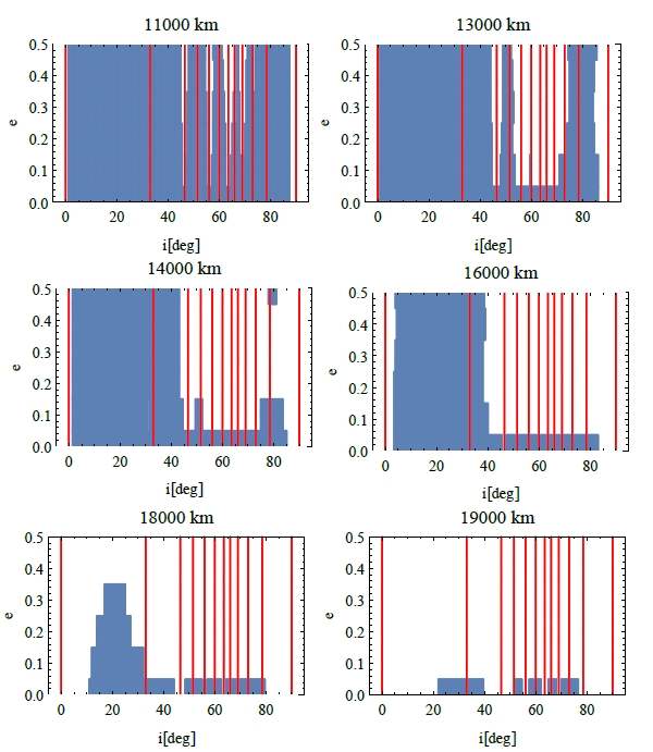
Figure 1. Domains of applicability of Theorem 2 for different values of the altitude. The blue regions represent the values of $(i_{*},e_{*})$ for which the Theorem can be applied, while the red lines define the values of the inclination which are associated with the most important resonances in the considered regions (see Table 2).

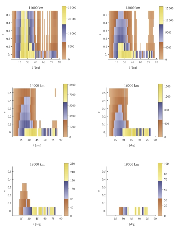
Figure 2. Stability time (in years) computed for the values of $(i_{*},e_{*})$ in the domain of applicability of Theorem 2.

At any rate, we stress that Theorem 2 used in the present work holds only for non-resonant domains in the phase space; therefore, by definition it cannot be used to probe the Nekhoroshev stability very close to resonances. We defer to a future study the question of the precise investigation of the conditions for Nekhoroshev stability inside resonances, by implementing a resonant form of the theorem, as first suggested in [Nek77].

4.2. Convergence of the preliminary normalization

As pointed out in Section 2.4, the aim of the preliminary normalization is to allow to control the norm of the perturbing function $|f_{\epsilon}|_{A,r_{0},s_{0}}$ by reducing the size of the complexified action domain $A_{r_{0}}$ (see (40)). In particular, the consequence of the removal of angle-dependent terms which are constant or linear in the actions is that, within certain values of the size of the domain $A_{r_{0}}$, the norm of the perturbation decreases quadratically with the actions.

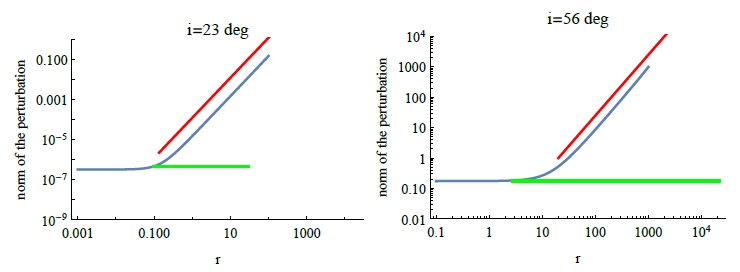
Figure 3. Blue: plot in $LogLog$ scale of $|f_{\epsilon}|_{A,r,s_{0}}$ for $a=13\,000$ km, $e_{*}=0.2$, and $i_{*}=23^{\circ}$ (left) and $i_{*}=56^{\circ}$ (right). For the computations, we selected $A=[P_{*}-r,P_{*}+r]\times[Q_{*}-r,Q_{*}+r]$, $r_{0}=r$, $s_{0}=0.1$. The slope of the plot for high $r$ is compared with that of a line with slope $2$ (red); the value at the plateau (denoted with a green line) is compared with the value of the norm of the purely trigonometric part of $f_{\epsilon}$ with $s_{0}=0.1$.

Figure 3 shows the behaviour of $|f_{\epsilon}|_{A,r,s_{0}}$ for $a=13\,000$ km, $e_{*}=0.2$ and two selected values of $i_{*}$, as a function of the size of the action in the complexified domain $A_{r}$ (the domain $A$ is set to be a rectangle of width $2r$ around the central values $P_{*}$ and $Q_{*}$). As expected, the value of $|f_{\epsilon}|_{A,r,s_{0}}$ decreases quadratically with $r$, until it reaches a plateau, whose value is the norm of the terms of $f_{\epsilon}$ which do not depend on the actions.

As already mentioned in Section 4.1, the convergence of the normalization presented in Section 2.4 for $\mathcal{H}^{(sec)}$ is crucial to control the size of the perturbing function $h_{1}$; such value plays a fundamental role in Theorem 2. A first study of the effect of the chosen value of the semimajor axis on the convergence can be performed by considering a simpler model to which a normalization procedure similar to the one implemented in Section 2.4 can be performed. The model is defined by the Hamiltonian

$$\tilde{\mathcal{H}}^{(in)}(P,Q,p,q)=\omega_{1}P+\omega_{2}Q+\frac{c_{2}}{2}Q^{2}+f_{1}\cos{q}\ ,$$ (49)

where the frequencies $\omega_{1}$, $\omega_{2}$ and the coefficient $c_{2}$ depend essentially only on the $J_{2}$ averaged Hamiltonian, while the coefficient $f_{1}$ depends on the lunar and solar third-body perturbation potentials, and it is proportional to the sinus of the inclination $i_{0}$ of the ecliptic. We will examine the effect of performing the preliminary normalization algorithm on the Hamiltonian $\tilde{\mathcal{H}}^{(in)}$ so as to remove purely trigonometric terms. After $N_{norm}$ normalization steps, the Hamiltonian takes the form:

$$\tilde{\mathcal{H}}^{(fin)}=\omega_{1}P+\omega_{2}Q+\frac{c_{2}}{2}Q^{2}+\sum_{\i=1}^{N_{norm}}Z_{i}(P,Q,q)+\sum_{i=N_{norm}+1}^{\infty}R_{i}(P,Q,q)\ ,$$ (50)

where the normalized parts $Z_{i}(P,Q,q)$ do not contain terms which depend only on the angle $q$ (as well as linear terms in the actions multiplied by trigonometric terms). By an explicit computation of the Poisson brackets involved in the normalization, we readily find that $R_{N_{norm}+1}$ contains trigonometric terms with coefficients proportional to the quantity

$$2^{a}f_{1}\left(\frac{c_{2}f_{1}}{4\omega_{2}^{2}}\right)^{N_{norm}},$$ (51)

where $a=1,2,3$ depends on the value of $N_{norm}$. The convergence of the remainder through the steps of the normalization algorithm depends, then, on the value of the ratio $c_{2}f_{1}/4\omega_{2}^{2}$; in particular, when this quantity is greater than 1, the normalization does not converge. Neglecting the lunar and solar contributions in $\omega_{1}$, $\omega_{2}$ and $c_{2}$, the coefficient $c_{2}f_{1}/4\omega_{2}^{2}$ can be expressed in terms of the orbital elements of debris, Sun and Moon as

$$\frac{c_{2}f_{1}}{4\omega_{2}^{2}}=\frac{1}{32}\frac{\sin{2i_{0}}}{R_{E}^{2}\mu_{E}J_{2}}\left(\frac{\mu_{M}}{(a_{M}(1-e_{M}))^{3}}+\frac{\mu_{\odot}}{(a_{\odot}(1-e_{\odot}))^{3}}\right)a^{5}(2+3e^{2}_{*})(1-e^{2}_{*})^{3/2}\tan{i_{*}}~{}~{}.$$ (52)

As a consequence, it is clear that its size strongly depends on $a$ and $i_{*}$: it grows sharply when $a$ increases and when $i_{*}$ approaches $90^{\circ}$.

On the other hand, the coefficient $f_{1}$ is proportional to $\sin{2i_{0}}$, that is, proportional to the (non-zero) inclination $i^{(p)}$ of the Laplace plane (see Eqs. (1) and (2)). Hence, the presence in the secular Hamiltonian of purely trigonometric terms is a manifestation of the presence in the model of a Laplace plane. Since $i^{(p)}$ increases with $a$ and $f_{1}$ increases both with $i^{(p)}$ and $i_{*}$, this gives a first explanation of the loss of stability of the model as $a$ and $i_{*}$ increase.

As already mentioned in Section 4.1, the other important factor influencing the size of the remainder across the preliminary normalization process is the effect of resonances, which, due to Eq.(37), leads to the appearance, in the series terms, of small divisors. Of particular importance are the small divisors appearing in the series’ purely trigonometric terms, whose size cannot be controlled by altering the size of the domain in the actions $A_{r_{0}}$.

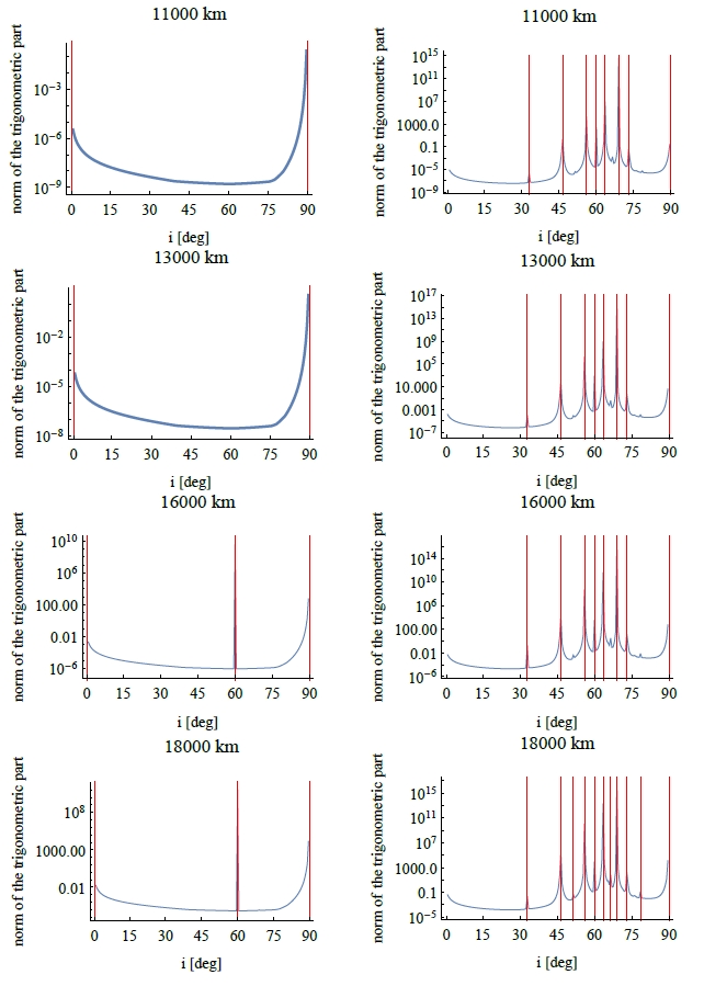
Figure 4. Behaviour of the norm of the purely trigonometric part of $h_{1}$ as a function of the inclination $i_{*}$ for different semimajor axes and eccentricities (left: $e=0$, right: $e=0.5$). The red lines represent the inclinations of the resonances (see Table 2).

Figure 4 shows the behaviour of the norm of the purely trigonometric part of the perturbation $h_{1}$ (with the notation (S3) of Section 3.2) as a function of the inclination for four different values of $a$ and two different values of $e$. As one can see, the size of the trigonometric part reaches its peaks in correspondence of the resonant values of the inclination, as expected. We also notice that the number of resonances involved in the growth of the size of the trigonometric part increases with $a$ and $e$.

As explained in Section 2.4, the normalization algorithm used in this work does not perform a re-tuning of the frequencies for every normalization step. This fact has important effects on the applicability of Theorem 2: when the normalization converges, the change between the original and the new frequencies is negligible with respect to their magnitude; on the other hand, when it does not converge, a large variation in the value of the frequencies occurs, with important consequences on the computation of $\alpha_{K}$ and, therefore, of the quantities involved in Theorem 2.

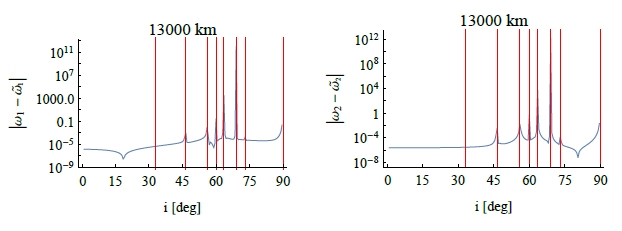
Figure 5. Variation between the initial ($\omega_{1}$ and $\omega_{2}$) and the final ($\tilde{\omega}_{1}$ and $\tilde{\omega}_{2}$)

frequencies as a function of the inclination $i_{*}$ for $a=13\,000$ km and $e_{*}=0.2$. The red lines represent the values of $i_{*}$ associated to the resonances which affect the convergence of the normalization algorithm (see Figure 4).

As an example, Figure 5 shows the variations of the frequencies as a function of the inclination for $a=13\,000$ km and $e_{*}=0.2$. Comparing Figures 4 and 5, it is clear that the resonances which affect the growth in size of the purely trigonometric part of $h_{1}$ and the variation of the frequencies are the same.

4.3. Behaviour of the cut-off value $\bar{K}$

$i_{*}(deg)$	$N(i_{*})$	$\bar{K}$	$i_{*}(deg)$	$N(i_{*})$	$\bar{K}$	$i_{*}(deg)$	$N(i_{*})$	$\bar{K}$	$i_{*}(deg)$	$N(i_{*})$	$\bar{K}$
46.5	1	0	89.5	1	0	1	2	1	63.5	2	0
33	3	2	73	3	0	56	3	0	38	3	3
53	4	1	78.5	4	3	40.5	4	5	27	5	4
51.5	5	4	58.5	5	0	69	5	0	81.5	5	4
41.5	6	5	50.5	6	5	83.5	6	4

Table 3. Comparison between the order $N(i_{*})$ of the nearest resonance and the computed cut-off value $\bar{K}$, computed for $a=13\,000$ km and $e=0.1$.

Provided that the classical normalization converges, from the definition of the cut-off value $\bar{K}$ given in Section 3.2, one expects that exactly at a resonance, once denoted with $N(i_{*})=|\alpha|+|\beta|$ its order, one has $\bar{K}=N(i_{*})-1$. Since in this work the inclinations are selected in a mesh of $[0,89.5^{\circ}]$ with step $0.5^{\circ}$, the computations of the quantities involved in Theorem 2, including $\bar{K}$, are not performed exactly at resonance (with the exception of $i_{*}=60^{\circ}$, whose distance from the exact resonance is of the order of $10^{-3}$): Table 3 shows the value of $\bar{K}$ computed for the points of the mesh which are near to the resonances up to order $6$, with $a=13\,000$ km and $e=0.1$, along with the resonance order $N(i_{*})$ of the nearest one. With the exception of the inclinations associated to resonances which affect the convergence of the classical normalization, the majority of the listed inclinations follows the expected rule $\bar{K}=N(i_{*})-1$, while some slight deviation is probably due to the numerical computation.

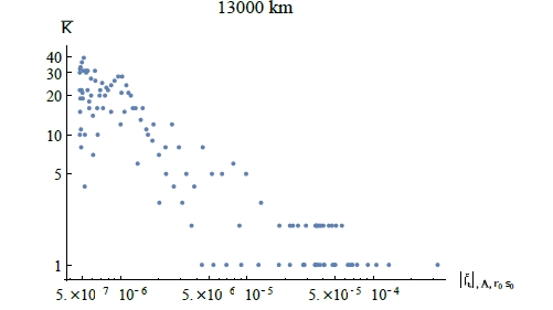
Figure 6. Plot in $LogLog$ scale of the points $\{|f_{\epsilon}|_{A,r_{0},s_{0}},\bar{K}\}$ for $a=13\,000$ km, $e_{*}=0.2$ and $i_{*}\in[0,90^{\circ}]$ on a mesh of step $0.5^{\circ}$.

To conclude, Figure 6 shows the relation between the computed values of $\bar{K}$ and $|f_{\epsilon}|_{a,s_{0},r_{0}}$ for $a=13\,000$ km, $e_{*}=0.2$ and $i_{*}\in[0,90^{\circ}]$. As expected, the cut-off decreases exponentially with the norm of the perturbing function.

Acknowledgements. A.C. partially acknowledges the MIUR Excellence Department Project awarded to the Department of Mathematics, University of Rome Tor Vergata, CUP E83C18000100006. A.C. and C.E. were partially supported by the Marie Curie ITN Stardust-R, GA 813644 of the H2020 research and innovation program. C.E. acknowledges the MIUR-PRIN 20178CJA2B “New Frontiers of Celestial Mechanics: theory and Applications”.

Appendix A Analytical expressions of $\mathcal{H}_{b}^{(av)}$ and $\mathcal{H}^{(sec)}$ in Section 2

A.1. Expansion of $\mathcal{H}_{b}^{(av)}$

We provide an expression of $\mathcal{H}_{b}^{(av)}$ for a third body (index $b$, referring to the Moon or Sun) as a function of its orbital parameters $(a_{b},e_{b},i_{b},\omega_{b},\Omega_{b})$ and the debris’ parameters $(a,e,i,\omega,\Omega)$. Up to second order in the eccentricity we have:

$$\begin{split}&\mathcal{H}_{b}^{(av)}=\frac{a^{2}}{16a_{b}^{3}(1-e_{b}^{2})^{3/2}}\Bigg{(}-\frac{2+3e^{2}}{8}(1+3\cos{(2i)})(1+3\cos{(2i_{0})})+\\ &-\frac{15}{4}e^{2}(1+3\cos{2i_{0}})\sin{i}^{2}\cos{2\omega}-\frac{3}{2}(2+3e^{2})\sin{i}^{2}\sin{i_{0}}^{2}\cos{2(\Omega-\Omega_{b_{0}})}+\\ &-15e^{2}\cos{(i/2)}^{4}\sin{i_{0}}^{2}\cos{2(\omega+\Omega-\Omega_{b_{0}})}-\frac{3}{2}(2+3e^{2})\sin{(2i)}\sin{(2i_{0})}\cos{(\Omega-\Omega_{b_{0}})}+\\ &+30e^{2}\cos{(i/2)}^{3}\sin{(i/2)}\sin{(2i_{0})}\cos{(2\omega+\Omega-\Omega_{b_{0}})}\\ &+\frac{15}{2}e^{2}(-1+\cos{i})\sin{i}\sin{i_{0}}\cos{(2\omega-\Omega+\Omega_{b_{0}})}+\\ &-15e^{2}\sin{(i/2)}^{4}\sin{(i_{0})}^{2}\cos{2(\omega-\Omega+\Omega_{b_{0}})}\Bigg{)}\ .\end{split}$$ (53)

A.2. List of the nonzero terms in $\mathcal{H}^{(sec)}$ for $j=1,2$

Assuming, as in Section 2, that both the lunar and solar orbits lie on a fixed ecliptic plane inclined with respect to the Earth’s equatorial plane by an angle $i_{0}$, the frequencies $\omega_{1}$ and $\omega_{2}$ appearing in (16) are given by:

$$\omega_{1}=\omega_{1}^{(J_{2})}+\omega_{1}^{(M)}+\omega_{1}^{(\odot)}\ ,\qquad\qquad\omega_{2}=\omega_{2}^{(J_{2})}+\omega_{2}^{(M)}+\omega_{2}^{(\odot)}\ ,$$

where

$$\omega_{1}^{(J_{2})} = -\frac{3}{4}R_{E}^{2}J_{2}\mu_{E}^{4}\frac{(-1+5\cos{i_{*}}^{2}-2\cos{i_{*}})}{(\mu_{E}a)^{7/2}(1-e_{*}^{2})^{2}}$$

$$\omega_{2}^{(J_{2})} = \frac{3}{2}\frac{R_{E}^{2}J_{2}\mu_{E}^{4}}{(\mu_{E}a)^{7/2}(1-e^{2})^{2}}\cos{i_{*}}$$

$$\omega_{1}^{(M/\odot)} = -\frac{3}{64}a^{3/2}\mu_{M/\odot}\frac{[3+2e_{*}^{2}-2(2+3e_{*}^{2})\cos{i_{*}}+5\cos{2i_{*}}](1+3\cos{2i_{0}})}{\sqrt{1-e_{*}^{2}}\sqrt{\mu_{E}}(a_{M/\odot}(1-e_{M/\odot}))^{3}}$$

$$\omega_{2}^{(M/\odot)} = \frac{3}{32}a^{3/2}\mu_{M/\odot}\frac{\left(2+3e_{*}^{2}\right)\cos{i_{*}}\left(1+3\cos{2i_{0}}\right)}{\sqrt{1-e_{*}^{2}}\sqrt{\mu_{E}}\left(a_{M/\odot}(1-e_{M/\odot})\right)^{3}}.$$ (54)

The coefficients $a_{\mathbf{l}}$ and $b_{\mathbf{l},\mathbf{k}}$ in (2.4) are given by:

$$\begin{split}a_{(2,0)}=&\frac{3}{4}\frac{J_{2}R_{E}^{2}}{a^{4}(1-e_{*}^{2})^{5/2}}(1+10\cos{i_{*}}-15\cos^{2}{i_{*}})+\\ &-\frac{3}{128}\frac{a}{\mu_{E}(1-e_{*}^{2})}\left(\frac{\mu_{M}}{R_{M}^{3}}+\frac{\mu_{\odot}}{R_{\odot}^{3}}\right)(1+3\cos{2i_{0}})(21+4e_{*}^{2}-40\cos{i_{*}}+15\cos{2i_{*}})\\ a_{(1,1)}=&\frac{3}{2}\frac{J_{2}R_{E}^{2}}{a^{4}(1-e_{*}^{2})^{5/2}}(5\cos{i_{*}}-1)+\\ &-\frac{3}{32}\frac{a}{\mu_{E}(1-e_{*}^{2})}\left(\frac{\mu_{M}}{R_{M}^{3}}+\frac{\mu_{\odot}}{R_{\odot}^{3}}\right)(1+3\cos{2i_{0}})(2+3e_{*}^{2}-10\cos{i_{*}})\\ a_{(0,2)}=&-\frac{3}{4}\frac{J_{2}R_{E}^{2}}{a^{4}(1-e_{*}^{2})^{5/2}}+\\ &-\frac{3}{64}\frac{a}{\mu_{E}(1-e_{*}^{2})}\left(\frac{\mu_{M}}{R_{M}^{3}}+\frac{\mu_{\odot}}{R_{\odot}^{3}}\right)(1+3\cos{2i_{0}})\left(2+3e_{*}^{2}\right)\end{split}$$

$$\begin{split}&b_{(0,0),(\pm 2,0)}=-\frac{15}{32}(a^{2}e_{*}^{2}\sin^{2}{i_{0}}\cos^{4}{(i_{*}/2)})\left(\frac{\mu_{M}}{r_{M}^{3}}+\frac{\mu_{\odot}}{r_{\odot}^{3}}\right)\\ &b_{(0,0),(\pm 2,\pm 1)}=\frac{15}{16}\left[a^{2}e_{*}^{2}\sin{(2i_{0})}\cos^{3}{(i_{*}/2)}\sin{(i_{*}/2)}\right]\left(\frac{\mu_{M}}{r_{M}^{3}}+\frac{\mu_{\odot}}{r_{\odot}^{3}}\right)\\ &b_{(0,0),(\pm 2,\mp 2)}=-\frac{15}{128}\left[a^{2}e_{*}^{2}(i+3\cos{(2i_{0})})\sin^{2}{i_{*}}\right]\left(\frac{\mu_{M}}{r_{M}^{3}}+\frac{\mu_{\odot}}{r_{\odot}^{3}}\right)\\ &b_{(0,0),(\pm 2,\mp 3)}=-\frac{15}{16}\left[a^{2}e_{*}^{2}\sin{(2i_{0})}\sin^{3}{(i_{*}/2)}\cos{(i_{*}/2)}\right]\left(\frac{\mu_{M}}{r_{M}^{3}}+\frac{\mu_{\odot}}{r_{\odot}^{3}}\right)\\ &b_{(0,0),(\pm 2,\mp 4)}=-\frac{15}{32}\left[a^{2}e_{*}^{2}\sin^{2}{i_{0}}\sin^{4}{(i_{*}/2)}\right]\left(\frac{\mu_{M}}{r_{M}^{3}}+\frac{\mu_{\odot}}{r_{\odot}^{3}}\right)\\ &b_{(0,0),(0,\pm 1)}=-\frac{3}{64}\left[a^{2}(2+3e_{*}^{2})\sin{(2i_{0})}\cos{(2i_{*})}\right]\left(\frac{\mu_{M}}{r_{M}^{3}}+\frac{\mu_{\odot}}{r_{\odot}^{3}}\right)\\ &b_{(0,0),(0,\pm 2)}=-\frac{3}{64}\left[a^{2}(2+3e_{*}^{2})\sin^{2}{i_{0}}\sin^{2}{i_{*}}\right]\left(\frac{\mu_{M}}{r_{M}^{3}}+\frac{\mu_{\odot}}{r_{\odot}^{3}}\right)\ .\end{split}$$

References

- [ADR+16] E. M. Alessi, F. Deleflie, A.J. Rosengren, A. Rossi, G.B. Valsecchi, J. Daquin, and K. Merz. A numerical investigation on the eccentricity growth of GNSS disposal orbits. Celest. Mech. Dyn. Astr., 125(1):71–90, 2016.
- [AHA21] J.M. Aristoff, J.T. Horwood, and K.T. Alfriend. On a set of equinoctial orbital elements and their use for uncertainty propagation. Celest. Mech. Dyn. Astr., 133(9), 2021.
- [Arn64] V.I. Arnold. Instability of dynamical systems with several degrees of freedom. Sov. Math. Doklady, 5:581–585, 1964.
- [BG86] G. Benettin and G. Gallavotti. Stability of motions near resonances in quasi-integrable Hamiltonian systems. Journal of Statistical Physics, 44(3-4):293–338, 1986.
- [Bre01a] S. Breiter. Lunisolar resonances revisited. Celest. Mech. Dyn. Astr., 81:81–91, 2001.
- [Bre01b] S. Breiter. On the coupling of lunisolar resonances for Earth satellite orbits. Celestial Mechanics and Dynamical Astronomy, 80(1):1–20, 2001.
- [CEG+17] A. Celletti, C. Efthymiopoulos, F. Gachet, C. Galeş, and G. Pucacco. Dynamical models and the onset of chaos in space debris. International Journal of Non-Linear Mechanics, 90:147–163, 2017.
- [Cel10] A. Celletti. Stability and Chaos in Celestial Mechanics. Springer-Verlag, Berlin; published in association with Praxis Publishing, Chichester, 2010.
- [CF96] A. Celletti and L. Ferrara. An application of Nekhoroshev theorem to the restricted three-body problem. Celest. Mech. Dyn. Astr., 64:261–272, 1996.
- [CG91] A. Celletti and A. Giorgilli. On the stability of the Lagrangian points in the spatial restricted problem of three bodies. Cel. Mech. Dyn. Astr., 50:31–58, 1991.
- [CG04] C.C. Chao and R.A. Gick. Long-term evolution of navigation satellite orbits: Gps/glonass/galileo. Advances in Space Research, 34:1221–1226, 2004.
- [CG14] A. Celletti and C. Gales. On the dynamics of space debris: 1:1 and 2:1 resonances. J. Nonlinear Science, 24(6):1231–1262, 2014.
- [CG18] A. Celletti and C. Galeş. Dynamics of resonances and equilibria of low Earth objects. SIAM Journal on Applied Dynamical Systems, 17(1):203–235, 2018.
- [CGL20] A. Celletti, C. Gales, and C. Lhotka. Resonances in the Earth’s space environment. Comm. Nonlinear Sciences and Numerical Simulations, 84:105185, 2020.
- [CGP16] A. Celletti, C. Gales, and G. Pucacco. Bifurcation of lunisolar secular resonances for space debris orbits. SIAM J. Appl. Dyn. Syst., 15:1352–1383, 2016.
- [CGPR17] A. Celletti, C. Gales, G. Pucacco, and A. Rosengren. Analytical development of the lunisolar disturbing function and the critical inclination secular resonance. Celest. Mech. Dyn. Astron., 127(3):259–283, 2017.
- [Coo62] G. E. Cook. Luni-solar perturbations of the orbit of an Earth satellite. Geophysical Journal International, 6(3):271–291, 1962.
- [CPL15] D. Casanova, A. Petit, and A. Lemaître. Long-term evolution of space debris under the effect, the solar radiation pressure and the solar and lunar perturbations. Celest. Mech. Dyn. Astr., 123:223–238, 2015.
- [DBCE21] I. De Blasi, A. Celletti, and C. Efthymiopoulos. Semi-analyitical estimates for the orbital stability of Earth’s satellite. J. Nonlinear Science, 31(93), 2021.
- [DRA+16] J. Daquin, A.J. Rosengren, E.M. Alessi, F. Deleflie, G.B. Valsecchi, and A. Rossi. The dynamical structure of the MEO region: long-term stability, chaos, and transport. Celestial Mechanics and Dynamical Astronomy, 124(4):335–366, 2016.
- [EH97] T.A. Ely and K.C. Howell. Dynamics of artificial satellite orbits with tesseral resonances including the effects of luni-solar perturbations. Dynamics and Stability of Systems, 12(4):243–269, 1997.
- [GDGR16] I. Gkolias, J. Daquin, F. Gachet, and A.J. Rosengren. From order to chaos in Earth satellite orbits. The Astronomical Journal, 152(5):119, 2016.
- [Gia74] G.E.O. Giacaglia. Lunar perturbations of artificial satellites of the Earth. Celest. Mech., 9:239–267, 1974.
- [GS97] A. Giorgilli and C. Skokos. On the stability of the Trojan asteroids. Astron. Astrophys., 317:254–261, 1997.
- [Hug80] S. Hughes. Earth satellite orbits with resonant lunisolar perturbations. i. Resonances dependent only on inclination. Proc. R. Soc. Lond. A, 372:243–264, 1980.
- [Kau62] W.M. Kaula. Development of the lunar and solar disturbing functions for a close satellite. Astron. J., 67:300–303, 1962.
- [Lan89] M. T. Lane. On analytic modeling of lunar perturbations of artificial satellites of the Earth. Celest. Mech. Dynam. Astr., 46(4):287–305, 1989.
- [LCG16] C. Lhotka, A. Celletti, and C. Gales. Poynting-Robertson drag and solar wind in the space debris problem. Mon. Not. Roy. Ast. Soc., 460:802–815, 2016.
- [LDV09] A. Lemaître, N. Delsate, and S. Valk. A web of secondary resonances for large geostationary debris. Celest. Mech. Dyn. Astr., 104:383–402, 2009.
- [Nek77] N.N. Nekhoroshev. An exponential estimate of the time of stability of nearly-integrable Hamiltonian systems. Uspekhi Matematicheskikh Nauk, 32(6):5–66, 1977.
- [NG21] T. Nie and P. Gurfil. Long-term evolution of orbital inclination due to third-body inclination. Celest. Mech. Dyn. Astr., 133(1), 2021.
- [Pös93] J. Pöschel. Nekhoroshev estimates for quasi-convex hamiltonian systems. Mathematische Zeitschrift, 213(1):187–216, 04 1993.
- [RARV15] A.J. Rosengren, E.M. Alessi, A. Rossi, and G.B. Valsecchi. Chaos in navigation satellite orbits caused by the perturbed motion of the moon. Mon. Not. R. Astron. Soc., 449:3522–3526, 2015.
- [RDT+16] A.J. Rosengren, J. Daquin, K. Tsiganis, E.M. Alessi, F. Deleflie, A. Rossi, and G.B. Valsecchi. Galileo disposal strategy: stability, chaos and predictability. Monthly Notices of the Royal Astronomical Society, 464(4):4063–4076, 2016.
- [Ros08] A. Rossi. Resonant dynamics of medium Earth orbits: space debris issues. Celestial Mechanics and Dynamical Astronomy, 100(4):267–286, 2008.
- [RS13] A.J. Rosengren and D.J. Scheeres. Long-term dynamics of high area-to-mass ratio objects in high-Earth orbit. Adv. Space Res., 52:1545–1560, 2013.
- [SRTV19] D.K. Skoulidou, A.J. Rosengren, K. Tsiganis, and G. Voyatzis. Medium Earth orbit dynamical survey and its use in passive debris removal. Advances in Space Research, 63(11):3646–3674, 2019.
- [VL08] S. Valk and A. Lemaître. Analytical and semi-analytical investigations of geosynchronous space debris with high area-to-mass ratios. Advances in Space Research, 41:1077–1090, 2008.