Achieving Low Complexity Neural Decoders via Iterative Pruning
Abstract
The advancement of deep learning has led to the development of neural decoders for low latency communications. However, neural decoders can be very complex which can lead to increased computation and latency. We consider iterative pruning approaches (such as the lottery ticket hypothesis algorithm) to prune weights in neural decoders. Decoders with fewer number of weights can have lower latency and lower complexity while retaining the accuracy of the original model. This will make neural decoders more suitable for mobile and other edge devices with limited computational power. We also propose semi-soft decision decoding for neural decoders which can be used to improve the bit error rate performance of the pruned network.
1 Introduction
Modern fifth generation (5G) communication systems require ultra-reliable low-latency communications (URLLC) [1]. This necessitates the use of low latency decoders which can infer the sent data from the received data quickly. Deep learning based function approximation approaches provide a natural way to side-step many of the computational complexities involved in various sub-parts of the communication pipeline, enabling low-latency communications [2, 3, 4, o2017, zheng2020deepreceiver, nachmani2018deep, kim2018communication]. Such approaches could thus potentially find use in mobile and other low-end devices which have limited computational power.
One such example of a deep learning based approach that has been explored is the use of neural networks for low-latency decoding [2, 3]. Typically, neural decoders for codes can either be single-label ( output nodes) or multi-label ( or output nodes). Here, represents the number of message bits, and represents the number of transmitted codeword bits. Thus single-label decoders become computationally unfeasible with larger , as opposed to multi-label decoders. However, as observed in [5], even for multi-label decoders, the desired network complexity increases substantially with larger , due to the larger dimensionality of the input space. As the primary goal of using these networks is to reduce computational complexity, there remains much scope for exploring ways to reduce complexity of these architectures while maintaining their decoding performance.
To address the issue of complexity, we explore a state-of-the-art approach for reducing neural network complexity while maintaining performance, namely the iterative network pruning approach proposed in [6], which uses the lottery ticket hypothesis (LTH). The lottery ticket hypothesis states that smaller sub-networks exist within the original network which can reach test accuracy comparable to the original model (or greater), when trained in isolation (in a similar number of iterations). In this paper, we apply the iterative pruning method in [6] to neural decoders for Hamming and polar codes, and find that we can substantially reduce the complexity of neural decoders (up to 97% pruning rates) while retaining their performance (test accuracy and Bit-Error Rate). Since the main purpose of the neural decoders is to correct errors introduced by the channel, we only consider neural decoders which predict the denoised codeword itself, i.e., using input and output nodes.111Note that for systematic codes, this is equivalent to a neural decoder that directly infers the message bits because the message bits can be directly inferred from the codeword bits. Additionally, we also propose a semi-soft decision decoding approach for neural decoders, which enhances the performance of a neural decoder while minimally increasing computational complexity.
Our work in this paper provides a platform for (i) further exploration of complexity reduction approaches such as the iterative-pruning approach in [6] for neural decoding, and (ii) also the use of computationally feasible extensions for neural decoders such as semi-soft decoding for improving decoding performance.
2 Background
In a communication system the transmitter encodes a message of bits into a code word of length n. This codeword is then sent over an additive white Gaussian noise (AWGN) channel to the receiver where it decodes the received vector of length to find out the original codeword (or message). In the optimal decoding strategy, also called maximum likelihood (ML) decoding, the receiver chooses the codeword which is closest (in terms of Euclidean distance) to the noisy received vector. Since the total number of codewords is , ML decoding needs to compare each received block to codewords, which grows exponentially with . To overcome the exponential decoding complexity of soft decision decoding, neural decoders can be used ([4]) to quickly produce an estimate of the sent codeword, eliminating the need to compare the received vector with all the valid codewords.
In this work, we also study one-shot pruning and the iterative pruning approach shown in [6] to reduce the complexity of our neural decoders. One-shot pruning removes a fraction of the weights after one round of training. In contrast, iterative pruning involves recursively pruning a small proportion of the network weights at the end of each iteration of training, which is invoked via the early stopping criterion mentioned in [6]. After the pruning step at the end of each training iteration, the rest of the un-pruned network weights are reset back to their initial values, after which the entire training and pruning process is repeated. It was shown in [6] that such an iterative pruning method can yield heavily pruned network configurations which can perform similar or better than the original network.
3 System Model
3.1 Communication Model
In the communication model, the transmitter encodes the message consisting of information bits, i.e., , to a codeword consisting of coded bits, i.e., . Each of the message bits can be either 0 or 1 with equal probability. Then, the transmitter modulates the codeword to get the modulated signal . These modulated bits are then sent over an AWGN channel to the receiver. At the receiver, a noisy corrupted form of the codeword is received, i.e., , where is the noise vector sampled from the multivariate Gaussian distribution . For an AWGN channel, , where denotes the identity matrix of size and is the power spectral density of the noise. The received vector is then fed into a neural network which outputs a prediction vector . We denote the rate of this code by . Moreover, the energy per message bit is given by .
3.2 Neural Decoder Architecture
The neural decoder consists of hidden layers with neurons each for . The input and output layers consists of neurons each, where is the codeword length. We use the ReLu function as the activation function for our hidden layers. Moreover, the sigmoid function is used as the activation function for the output layer. Here, the sigmoid functions restricts the output of the model to be between 0 and 1. which can be seen as the probability of the bit being 0 or 1 at one particular position. The model is trained with the loss function being the binary cross entropy function. Table 1 summarizes the parameters of the neural decoder.
| Layer | Activation Function |
|---|---|
| Input Layer () | None |
| Hidden Layer ( for ) | |
| Output Layer () |
4 Decoding Techniques
4.1 Hard Decision Decoding
To output a binary codeword, we use threshold based decoding, with threshold , on the neural decoder output of length . That is, for each bit position , we decide that the codeword bit at position is 0 if position of the output of the neural network is less than , else we decide that the bit at position is 1.
4.2 Semi Soft Decision Decoding
To improve the performance of the pruned network, we use soft decision decoding on a fixed number of the predicted codeword bits and do a hard decision (threshold) decoding on the rest. This approach, termed semi-soft decision decoding, is inspired by Chase decoding [7] and its variants [8]. First, for a received vector of length and for a fixed number , we find the "least confident bit positions" (which are closest to 0.5) of the output of the neural network. Then, we do threshold decoding on the rest of the bits and keep these bit positions the same. Let’s denote the prediction vector at this stage by . We now fill the remaining bits with all possible combinations of 0s and 1s and obtain a list of vectors. Now, using a hash table which consists of all the valid codewords, we can check for each of the possibilities, in time, whether they are present in the hash table. Having obtained all the valid codewords that match in the remaining positions, we can compare the euclidean distance of with each of the valid codewords that we just obtained and chose the codeword that is closest to to get the final estimated codeword as . Note that the maximum number of valid codewords that we can obtain using the hash table is . Hence, we can reduce the number of codewords ( instead of ) with which we have to compare the distance of the output of the neural network. In the case when there are no valid codewords for a given , we simply do a hard decision decoding the bits as discussed in Section 4.1. The complexity of this algorithm can be controlled by the receiver by specifying the .
5 Experiments
In this section, we conduct a series of experiments with neural decoders for Hamming (7,4) [9] and Polar (16,8) codes [10]. In the case of Hamming Codes, the BER is the fraction of message bits that are in error. For Polar Codes, we calculate the BER by finding the fraction of bits that are in error in the received codeword. The actual BER, which is the fraction of bits that are in error in the received message, may be slightly better owing to the fact that it is possible to have 0 errors in the estimated message even if there are some errors in the estimated codeword. In both cases, we first test the iterative pruning approach based on the LTH, and then test our proposed semi-soft decoding approach on the neural decoders. Unless mentioned otherwise, the training and testing SNR is 0 dB for Hamming Codes and 2 dB for Polar Codes. For what follows, we denote the optimal max-likelihood soft decision decoding approach as ML decoding, and the iterative pruning method is simply denoted as the LTH approach.
5.1 Hamming (7,4) Codes
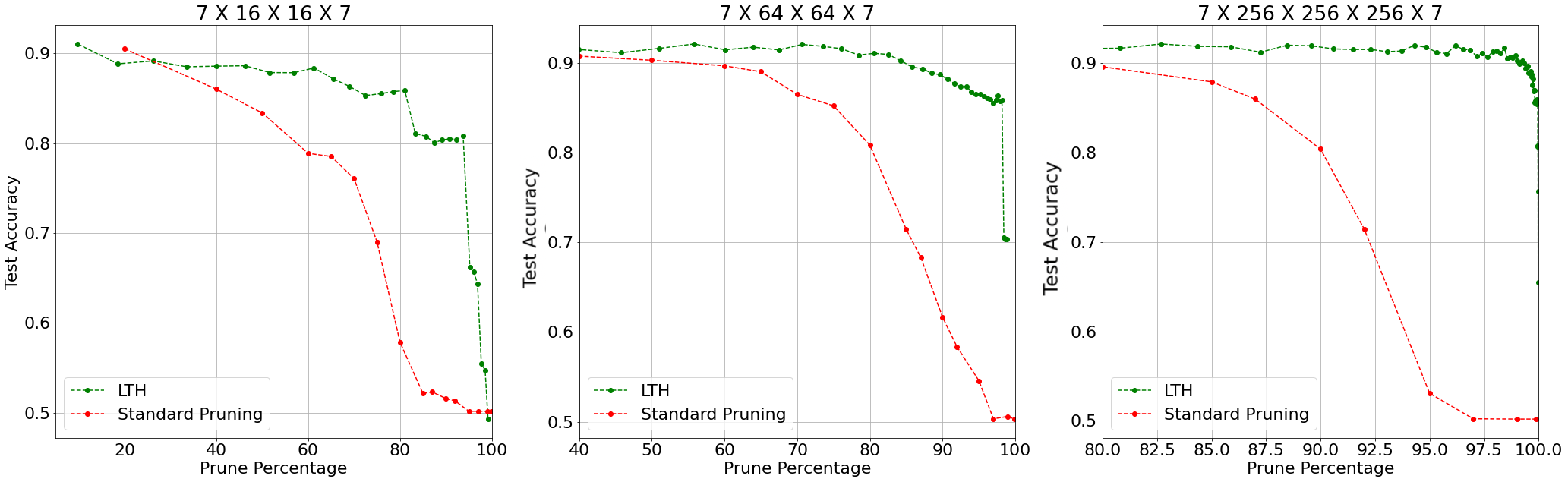
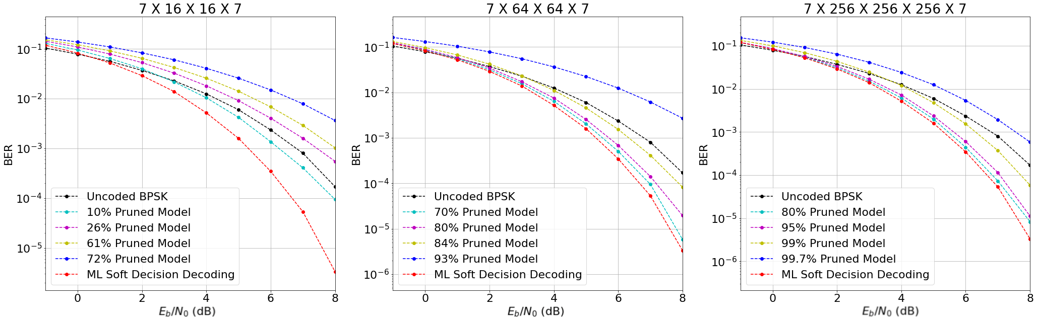
First, we test the LTH and the standard one-shot pruning approaches with neural decoders for Hamming (7,4) codes. Figure 1 shows how the test accuracy changes in response to increasing levels of pruning, for three network configurations having varying levels of complexity. The network configurations are written at the top of the plots in the following format: for . We note that in all cases, the LTH outperforms standard pruning by a significant margin, while retaining the accuracy of the original model for a wide range of pruning. Figure 2 shows the performance of the pruned network at various stages of pruning. By comparing Figure 1 and Figure 2, we see that for the neural decoder to reach ML decoding level performance, the test accuracy in Figure 1 must be around 90%. For the case of the decoder with the configuration of = 64 for , we see that it can closely approximate the optimal ML Decoding when 80% pruned. Interestingly, we consistently find that heavily pruned complex network configurations usually fare better than lightly pruned network configurations of less complexity.
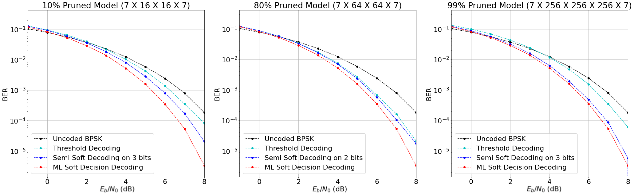
Next, in Figure 3, we show the effect of the proposed semi-soft decision decoding method on the BER performances of pruned neural decoders. As can be seen from the figure, semi-soft decision decoding provides a noticeable improvement in the BER of the neural decoders even when is as small as 2 and 3. Moreover, we see a significant level of improvement for heavily pruned models, which originally have poor BER performance.
5.2 Polar (16,8) Codes
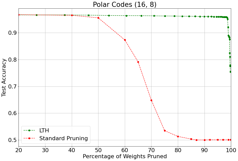
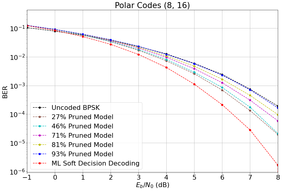
We now test the LTH pruning approach with neural decoders for Polar (16,8) codes. Figure 4a shows the observed test accuracies at 2 dB SNR, in response to varying levels of network pruning. Like before, we see that LTH retains the test accuracy of the original un-pruned network for a very wide range of pruning levels, and significantly outperforms standard pruning approaches. The BER curves of the various pruned network configurations are shown in Figure 4b. In this case, we find that slight differences in the test accuracy at 2 dB SNR get amplified for higher SNR levels. For example, the 93% pruned network is found to have only slightly lower test accuracy than less pruned configurations in Figure 4a, but yields significantly worse BER in Figure 4b.
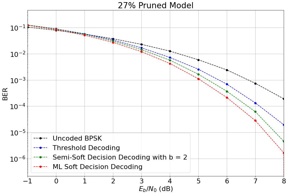
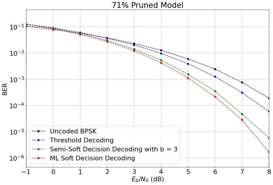
Next, we test the impact of the proposed semi-soft decoding approach on the BER performances of the pruned networks. Results are shown in Figures 4c and 4d. Like before, we find that semi-soft decoding significantly enhances BER performances for the pruned neural decoders, for and , enabling near optimal decoding.
6 Discussions and Conclusions
Our work establishes that iterative pruning approaches motivated by the lottery ticket hypothesis can reduce the complexity of neural decoders manyfold (up to 97%), while maintaining decoding performance. This is verified across multiple experiments conducted with Hamming (7,4) and Polar (16,8) codes. We also study a semi-soft decision decoding approach on the neural decoder outputs, which improves decoding performance in all cases.
Apart from the approaches demonstrated here, we are also investigating network weight quantization methods for reducing network complexity. We find that quantization can reduce network sizes up to a factor of 4, while maintaining performance. Through our initial investigative studies here, we hope to spark further research into combining pruning, semi-soft decoding and quantization based approaches for creating efficient low complexity neural decoders suitable for use in low-end communication edge devices.
Acknowledgments
This work was supported in part by the Singapore Ministry of Education under Grant MOE2019-T2-2-171.
References
- [1] Gordon J Sutton, Jie Zeng, Ren Ping Liu, Wei Ni, Diep N Nguyen, Beeshanga A Jayawickrama, Xiaojing Huang, Mehran Abolhasan, Zhang Zhang, Eryk Dutkiewicz, et al. Enabling technologies for ultra-reliable and low latency communications: From phy and mac layer perspectives. IEEE Communications Surveys & Tutorials, 21(3):2488–2524, 2019.
- [2] Cheuk Ting Leung, Rajshekhar V Bhat, and Mehul Motani. Low-latency neural decoders for linear and non-linear block codes. In 2019 IEEE Global Communications Conference (GLOBECOM), pages 1–6. IEEE, 2019.
- [3] Cheuk Ting Leung, Mehul Motani, and Rajshekhar V Bhat. Multi-label and concatenated neural block decoders. In 2020 IEEE International Symposium on Information Theory (ISIT), pages 274–279. IEEE, 2020.
- [4] Cheuk Ting Leung, Rajshekhar V Bhat, and Mehul Motani. Multi-label neural decoders for block codes. In ICC 2020-2020 IEEE International Conference on Communications (ICC), pages 1–6. IEEE, 2020.
- [5] Nghia Doan, Seyyed Ali Hashemi, and Warren J Gross. Neural successive cancellation decoding of polar codes. In 2018 IEEE 19th international workshop on signal processing advances in wireless communications (SPAWC), pages 1–5. IEEE, 2018.
- [6] Jonathan Frankle and Michael Carbin. The lottery ticket hypothesis: Finding sparse, trainable neural networks. arXiv preprint arXiv:1803.03635, 2018.
- [7] David Chase. Class of algorithms for decoding block codes with channel measurement information. IEEE Transactions on Information theory, 18(1):170–182, 1972.
- [8] Hsin-Kun Lai and Erl-Huei Lu. Semi-soft decision decoding based on correspondence between error patterns and the relative test patterns. In Second International Conference on Innovative Computing, Informatio and Control (ICICIC 2007), pages 396–396. IEEE, 2007.
- [9] Shu Lin and Daniel J Costello. Error control coding, volume 2. Prentice hall Scarborough, 2001.
- [10] Erdal Arikan. Channel polarization: A method for constructing capacity-achieving codes for symmetric binary-input memoryless channels. IEEE Transactions on information Theory, 55(7):3051–3073, 2009.