Using machine learning to auto-tune chi-squared tests for gravitational wave searches
Abstract
The sensitivity of gravitational wave searches is reduced by the presence of non-Gaussian noise in the detector data. These non-Gaussianities often match well with the template waveforms used in matched filter searches, and require signal-consistency tests to distinguish them from astrophysical signals. However, empirically tuning these tests for maximum efficacy is time consuming and limits the complexity of these tests. In this work we demonstrate a framework to use machine-learning techniques to automatically tune signal-consistency tests. We implement a new signal-consistency test targeting the large population of noise found in searches for intermediate mass black hole binaries, training the new test using the framework set out in this paper. We find that this method effectively trains a complex model to down-weight the noise, while leaving the signal population relatively unaffected. This improves the sensitivity of the search by for signals with masses . In the future this framework could be used to implement new tests in any of the commonly used matched-filter search algorithms, further improving the sensitivity of our searches.
I Introduction
Since the first detection of gravitational waves in 2015 [1], the LIGO detectors have been upgraded multiple times, and the network of detectors now includes Advanced LIGO [2], Advanced Virgo [3] and Kagra [4]. The third observing run of the LIGO-Virgo-Kagra network [5] has been completed and a whole suite of new compact binary coalescence (CBC) signals have been observed [6, 7, 8, 9, 10, 11]. Along with improvements in the detectors, search algorithms used to search for CBC signals have also been improved by using information from the full network and introducing new methods for removing noise [12, 13, 14].
A set of modelled [15, 16, 17, 12, 18, 19, 13, 14, 20, 21, 22, 23, 11] and unmodelled [24] search algorithms have been used to observe CBCs in the past. In this paper we will focus on modelled searches. Modelled searches construct a large bank of simulated signals (templates) with a variety of masses and spins in order to cover the targeted parameter space. These templates are then each used to perform a matched filter over the data for each detector. The matched filter signal-to-noise ratio (SNR) is then compared across the detector network in order to check for consistency across detectors.
The matched filter is the optimal solution when searching for known signals assuming that only Gaussian noise is present [15]. However, in the presence of non-Gaussian noise transients, large SNRs can be produced where no signal is present [16]. Gravitational-wave detectors contain many such transients [25, 26], commonly referred to as “glitches”. Glitches can produce huge values of SNR while having little resemblance to the CBC signals being searched for. It is therefore necessary to employ signal-consistency tests to remove as many of these glitches as possible in order to reduce the rate of false alarms. In this paper we will explore how to effectively develop and tune such a signal-consistency test to separate the signal and noise populations. We will apply this methodology to the PyCBC search [12] as a demonstration of its use. However, we strongly emphasize that this method will be applicable to any modelled search.
In the PyCBC search, multiple signal-consistency tests are employed. Firstly, the matched filter SNR is modified using two tests that compare the morphology of the signal in the data with that of the template [27, 28], penalising any signals found to be inconsistent. Peaks in the re-weighted SNR time-series are then compared across the detector network, checking for consistency in the template parameters, as well as the relative time of arrival, amplitude and phase of the signals [29]. Each potential candidate event is then given a detection statistic in order to rank the likelihood that it is a real signal.
After these tests are performed, the remaining signals are shifted in time relative to each other to empirically measure a non-astrophysical background. The detection statistic values of the background signals can then be compared to the observed coincident signals in order to produce a false alarm rate for each observed signal [17].
The existing signal consistency tests remove a large number of glitches from the single detector data, reducing the rate of background coincidences, and therefore reducing the false alarm rate of observed signals. However, a large number of glitches continue to be detected, particularly when searching with high mass templates [30], , where the signal may only be in the detector frequency band for a fraction of a second.
In this work we propose a method of creating and tuning new signal-consistency tests in order to separate signal and noise populations. We show that we can use machine-learning techniques such as stochastic gradient descent to optimise these tests efficiently, and thus improve the sensitivity of our searches to gravitational wave signals.
The use of machine-learning in gravitational wave searches is an area where much work is being done. Several works have explored the use of neural networks to replace the matched filter statistic [31, 32, 33, 34, 35], using convolution neural networks to predict the probability of a signal being present.
One advantage of convolution neural networks compared to a matched filter is the computational cost involved. This is particularly important for multi-messenger astronomy, where prompt detection of gravitational wave signals could enable follow-up with electromagnetic observations. It has been shown that convolution neural networks could be an effective method for enabling such observations [36, 37, 38, 39, 40, 40].
These works have shown that machine-learning can, in some cases, compete with the sensitivity of a matched filter search when applied to a single detector. However, such methods have not yet been demonstrated to be effective in large-scale searches for CBCs covering a wide range of parameters. Current methods also do not produce additional information such as the amplitude and phase of the signal, used in the matched filter search to test triggers across detectors, they therefore lose sensitivity when compared to a matched filter search using a network of detectors [41].
In this work we choose to introduce a machine learning model within the current matched filter framework in order to utilise the statistical tests already available to us. We implement a new test using stochastic gradient descent to train a set of tunable parameters within the model, optimising the test using noise triggers from a previous search along with a set of simulated signals. By implementing the model as a test it should remain rigorous in the case of unseen data, such as a new population of glitches.
We start by describing the general use of tests within gravitational wave searches, and the tests currently used within the PyCBC search in Sec. II. In Sec. III we describe our proposed framework for training new tests using machine-learning methods. We then utilise this framework in Sec. IV to train a new test for use in a search for intermediate mass black holes (IMBHs). In Sec. V we present the effect of this trained model on the IMBH search showing that it improves the sensitivity of the search, particularly at high masses, where the effect of non-Gaussian noise is most prominent.
II A Review of Tests in GW Searches
We will begin by reviewing existing signal-consistency tests used in gravitational wave searches.
In order to search for signals in strain data, a matched filter is used. Assuming the strain data takes the form of , where is stationary Gaussian noise and is a known signal, matched filtering is the optimal method for detecting the signal . The calculated SNR is analytically maximised over the amplitude and phase of the signal. The SNR is calculated as:
| (1) |
where the inner product is:
| (2) |
and is the one-sided power spectral density (PSD) of the noise. However, in the case of non-Gaussian noise, large peaks in the SNR time-series can be produced. Short bursts of non-Gaussian noise are often referred to as “glitches”, these can produce extremely large values of SNR with little similarity to the signal being searched for. In order to remove such triggers signal-consistency tests may be introduced to test the morphology of the trigger compared to that of the search template.
A test is one such test. A test is constructed by performing a matched filter with additional templates, , that are orthogonal to the search template such that . Given well-behaved noise, and a signal which is an exact match to the search template, the matched filter SNR of the orthogonal template will follow a reduced distribution with 2 degrees of freedom [15]. However, when there is non-Gaussian noise present, such as a glitch, the SNR will deviate from this distribution, taking a larger value. By examining triggers on the SNR- plane the signal and noise populations may then be separated.
After choosing a suitable template, , to be used for the test one first normalises it so that . The part of the signal orthogonal to the search template is then selected:
| (3) |
N such templates are created in this way and their SNRs are combined to produce the statistic.
| (4) |
In the case that the templates are orthogonal to one another this will produce a reduced distribution with degrees of freedom. However, in general, orthogonality between the templates is not always enforced, in which case the statistic will follow a generalised distribution with increased variance.
The test also assumes that the signal in the data matches the search template. However, due to the discrete placement of templates within the parameter space of the search there will be some mismatch between these two signals. This mismatch means that the template will no longer be orthogonal to the signal and some of the signal’s SNR will be included in the statistic, increasing the mean of the distribution, creating a non-central distribution. A similar effect will be caused if the PSD is miscalculated, or if the noise is non-stationary.
In general any N templates can be chosen to construct a test. However, this test will be most effective when templates are chosen that have some overlap with known non-Gaussian noise in the data, in particular, aiming to target noise which produces high SNR triggers for the targeted parameter space.
To separate the signal and noise populations a re-weighted SNR is then calculated that penalises triggers where the is larger than expected. This re-weighting takes the general form
| (5) |
This re-weighted SNR is then used to rank potential candidate events.
II.1 Existing Tests in the PyCBC search
There are currently two signal-consistency tests employed within the PyCBC search. The first of these is the Allen test [27]. This test divides the template into independent frequency bins, splitting the template such that each bin will contribute equally to the SNR. The SNR contribution for each of these sub-templates is calculated and compared to the expected value, calculating the statistic as
| (6) |
This will take large values when a glitch is present in the data that does not share the same morphology as the search template. Specifically this test checks the distribution of power along the track of the CBC signal. Although this test does not follow the exact form described in the previous section, it follows the same principle detecting excess power along the track of the signal. The re-weighted SNR [42] is then calculated as
| (7) |
By ranking the candidates based on this re-weighted SNR, a large number of noise triggers can be down-weighted. This test is particularly powerful for lower mass systems where the signals span a wide range of frequencies within the band of the detectors, allowing for a larger number of frequency bins to be used effectively. The number of frequency bins to be used is varied as a function of the search templates parameters [43]. The number of frequency bins to use and the form of the SNR re-weighting are currently tuned empirically and have evolved over time [44, 42, 43].
The second test is the sine-Gaussian test [28]. This works by performing a matched filter with sine-Gaussian signals, each being placed at frequencies higher than those expected from the search template. As these sine-Gaussian signals do not overlap with the search template, we can construct a test as the sum of their SNRs
| (8) |
This statistic tests if excess power is present above the final frequency of the search template. When excess power is present large values of will be produced and the SNR is re-weighted again
| (9) |
The addition of this second test further reduces the rate of noise triggers due to glitches. This test has a significant impact for higher mass templates where there is a population of short duration glitches known as “blips” [45]. A subset of these blips have power extending to high frequencies allowing this test to remove them successfully [28]. However a large number of these glitches are not removed by this test [30].
Both of these tests have been tuned empirically by hand, choosing the number of frequency bins to be used and the placement of the sine-Gaussian signals, as well as the exact form of the re-weighting of the SNR. In the next section we propose an approach that allows us to create and tune new tests using a data-driven approach.
III Auto Tuning of a signal-consistency test
We propose a framework in which we create new tests and empirically tune them based on a set of training data. To achieve this we take a set of noise triggers from a previous search along with a set of simulated signals and use stochastic gradient descent to tune the parameters of our model.
In order to optimise the parameters of our chosen model we first must define a loss function, this is the quantity that we aim to minimise during the training process. The loss function is a function of the triggers SNR, , and its SNR re-weighted by the new test described in Sec. IV, . For this work we choose to define a separate loss function for noise triggers and simulated signals. The loss functions used in the case of noise triggers is,
| (10) |
which penalises any cases where the re-weighted SNR is greater than 4. Below this threshold the PyCBC search currently discards all triggers so it is unnecessary to reduce it any further.
The loss function used for simulated signals is:
| (11) |
This penalises the case where the value is large and the SNR is reduced. This contribution to the loss will also allow us to train a function that re-weights the SNR as in Eq. 5 in order to create a greater separation between the signal and noise populations in the SNR- plane.
To update the parameters of the model we must then calculate the gradients with respect to the loss function. This is done using backpropogation after calculating the loss function using a set of training data. The model and matched filter are implemented in Tensorflow[46, 47], allowing the gradients to be tracked through the calculation and the parameters updated.
Stochastic gradient descent has been used widely in the field of deep learning to optimise extremely complex models [48, 49], this framework therefore allows us to produce highly complex transformations while allowing us to effectively tune them to the detector data at a reasonable computational cost.
In the next section we will describe one such model and the data used to train the model.
IV A test for intermediate mass black hole searches
To demonstrate the training scheme described in the previous section we will attempt to train a test that improves the separation between glitches and signals when searching for IMBHs, which we consider as signals with . In this mass range the Allen test described in the Sec. II.1 has a limited effect due to the systems merging at low frequencies and covering a relatively small frequency range within the detector bandwidth. The sine-Gaussian test is successful in removing a population of glitches that affect templates within this mass range, however, many glitches remain that do not have significant high frequency power [30].
In this section we will define a transformation using the framework outlined in the previous sections using data from a previous IMBH search in order to train the test and improve the sensitivity of the search.
IV.1 Creating templates
Existing tests effectively test the distribution of power of a candidate event along the track of the signal in the time-frequency plane and test for excess power at high-frequencies. We aim to test for excess power in a frequency band similar to those of the search templates, aiming to cover areas of the time-frequency plane not currently covered by existing tests.
To achieve this we transform the search template itself, shifting the template in time and frequency. The optimal values for these time and frequency shifts will depend on the template being used and the noise present in the data. Time shifted templates have previously been used in the PyGRB search [50, 51] to create a signal-consistency test using fixed values for the time shifts. We propose a model that allows different time and frequency shifts for each template, tuning these values based on the current data.
The time and frequency shifts are selected using a dense neural network. The template is first turned into an input by sampling it between 12 Hz and 256 Hz with a sample width of 0.1 Hz, we then take the absolute value of the template and normalise it so that the mean of the input is one. This input is then passed to a dense neural network with two output values between -1 and 1. The first of these values is used as the time shift after being scaled by the maximum allowed time shift , similarly, the second value is used as the frequency shift after being scaled by the maximum allowed frequency shift .
The dense neural network consists of 11 dense layers, using the Rectified Linear Unit (ReLu) activation functions for hidden layers and the hyperbolic tangent function for the output layer. In order to produce multiple time/frequency shift pairs we train multiple networks with this configuration. However, to speed up the training of this model the first 6 dense layers are shared between each network. The sizes of the dense layers are listed in Table. 1.
| Layer | Output Size | |
|---|---|---|
| Input | 2440 | |
| Dense + ReLu | * | 128 |
| Dense + ReLu | * | 128 |
| Dense + ReLu | * | 64 |
| Dense + ReLu | * | 64 |
| Dense + ReLu | * | 32 |
| Dense + ReLu | * | 32 |
| Dense + ReLu | 16 | |
| Dense + ReLu | 16 | |
| Dense + ReLu | 8 | |
| Dense + ReLu | 8 | |
| Dense + tanh | 2 |
After calculating these shifts they are applied to the template before using Eq. 3 to generate our templates.
In addition to this model we must define a function to re-weight the SNR with the value. We create a parameterised model that can reproduce the re-weighting in Eq. 7 and 9.
| (12) |
Here , , and are parameters that can also be tuned to increase the effectiveness of the test. This re-weighting leaves any signals with less than the threshold, , unchanged. At large values and determine how quickly the re-weighted SNR decreases with the value, while and effect the transition between these two regimes.
IV.2 Data
In order to most effectively train the model we target glitches that are missed by previous signal-consistency tests. We achieve this by performing a search using the setup described in [30] covering days of data from the first half of the third observing run. The data used in this search is available from GWOSC [52, 53]. From this search we then select a set of noise triggers with and . These noise triggers may have been down-weighted by existing signal-consistency tests, but have not been down-weighted enough to remove them from the analysis. In order to avoid including real signals we remove any triggers that are coincident across multiple detectors. This will also remove a number of noise triggers that have formed coincident triggers, however, enough triggers remain to create a substantial training set. These triggers are then clustered over a window of 1 second and the triggers with the largest in that window are kept. We record the times of the triggers and the parameters of the template that produced them.
We also select a set of simulated signals to include during training. From the list of simulated signals that were recovered by the search, with false-alarm rates smaller than 1 per year, we select a set using the same constraints as the noise triggers. For these triggers we record the parameters of the simulated signal, as well as the template that recovered the signal. By using the template that recovered the signal in the search we are including the effect of template mismatch within the training scheme, this allows the SNR re-weighting step in Eq. 12 to be tuned to account for this contribution. The simulated signals used in this analysis include effects from precession and higher-order modes that are not present in the template bank, by including these effects in the analysis we can train the model to avoid identifying these effects as noise, maintaining our sensitivity to these signals.
For each sample, the strain is loaded at 2048Hz, for samples containing simulated signals the signal is then added. The strain data is high-pass filtered at 12Hz and PSDs are calculated using 512 seconds of data around the time of the sample, following the same procedure as the PyCBC search. 64 seconds of data around the trigger is then selected, ensuring the trigger is not within the first 32 seconds or the last 16 seconds to allow time for the inspiral and ringdown of the search templates.
The search templates are generated using the SEOBNRv4_ROM [54, 55] waveform model, and are generated at the same length and sample frequency as the strain data. The simulated signals are generated using the NRSur7DQ4 [56], SEOBNRv4 [54, 55] and SEOBNRv4HM [57, 58] waveform models.
In order to ensure the noise and signal samples have similar importance during training we select an equal number of each. Additionally, to ensure that the parameters in Eq. 12 are trained to separate the noise and signal populations across a range of SNRs we bin our samples by SNR and select an equal number of samples from the noise and signal models for each bin. The boundaries of these SNR bins are 6, 8, 10, 14, 18, 24 and 64. In each of these SNR bins we draw 1200 noise samples and signal samples from those remaining after filtering has been applied.
We set aside 10% of all samples to be used as a validation set to monitor the performance of the model on unseen data, all other samples are used to train the model. This gives us a total of 12960 samples for training and 1440 samples for validation.
IV.3 Training
The training of the model is performed in batches, each batch contains 32 samples from the training set described in the previous section. For each sample the peak SNR within 0.1 seconds of the trigger time is calculated. The search template is then generated and passed to the transformation described in Sec. IV.1. The resulting templates are then normalised and the orthogonal templates calculated using Eq. 3. These templates are then used to calculate at the time of the peak SNR and the re-weighted SNR is calculated. This value can then be passed to the loss function in order to calculate the loss values for the batch.
Once the losses have been calculated, backpropogation is used to obtain the gradients of the loss function with respect to the trainable weights of the network described in Sec. IV.1, as well as the trainable parameters in Eq. 12. Stochastic gradient descent is then used to apply small changes to the variables based on the calculated gradients. In order to speed up training and improve performance for sparse gradients we use Nesterov momentum [59] when calculating the parameter updates.
Before training the full model we perform a pre-training phase where only the parameters of the SNR re-weighting in Eq. 12 are trained. This step is faster than the training of the full model and by performing this step first the training of the model is more effective early in the training. After this step we proceed with the main training step, training the parameters of the model described in Sec. IV.1 and the SNR re-weighting in Eq. 12 at the same time.
The main training step is repeated until all samples in the training set have been analysed 25 times, taking a total of hours using 8 CPU cores. During training the learning rate determines how quickly parameters are changed in response to the calculated gradients. In order to improve convergence late in the training stage we employ learning rate decay. After each full cycle of the training set the learning rate is multiplied by a factor of 0.9, allowing the model to make smaller adjustments late in training.
IV.4 Trained Model
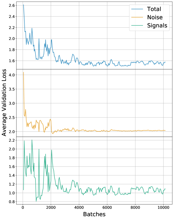
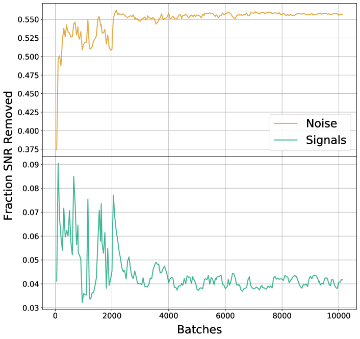
As shown in Fig. 1 we see that the loss calculated using the test set decreases as training continues. This change is mainly driven by the model down-weighting noise triggers, while the contribution from signals makes a smaller change over the course of the training. The effect of this training can also be seen in Fig. 2, we can see that as training continues a larger fraction of the SNR is removed as noise triggers are targeted more effectively by the model, while signals are left relatively unaffected.
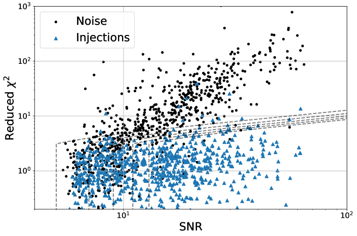
In Fig. 3 we can see that the noise and signal populations are well separated in the SNR- plane, particularly at high SNRs. The parameters in Eq. 12 have been trained such that the majority of signal samples are below the threshold, , while noise samples above the threshold are heavily down-weighted.
The trained parameters are available as a supplementary data file at: https://icg-gravwaves.github.io/chisqnet/
V Effect on a Intermediate Mass Black Hole Search
In this section we will show the effect of introducing this model to a search for IMBHs. For this test we carry out a search following the configuration set out in [30], covering days of data from the first half of the third observing run. We run the search twice, with the only change being the introduction of the model trained in the previous section. To ensure that the model generalises to new data we run this search on a stretch of data completely separate to that used during training.
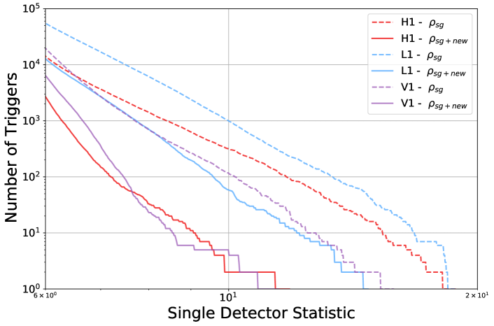
By introducing this model, noise triggers can be effectively down-weighted. Fig. 4 shows the change in the number of triggers found when using the new ranking statistic. This reduction in triggers will reduce the number of coincident noise triggers in the foreground and the empirically measured background. It is this decrease in the rate of background triggers that produces an increase in the significance of remaining foreground triggers, thereby improving the sensitivity of the search.
We evaluate the sensitivity of the search using a number of simulated signals added to the data and analysed in the same way as the main search. These simulated signals follow the same distribution as those in [30]. The SEOBNRv4 and SEOBNRv4HM waveform models are used to generate aligned spin signals, with total masses in the range and mass ratios in the range . Precessing signals are generated using the NRSur7DQ4 waveform model with total masses in the range , mass ratios in the range and component spins isotropically distributed. For all simulated signals the distance is drawn uniformly in the range Gpc, with isotropic sky positions and binary orientations. The sensitive volume of the search is then calculated by applying a threshold to the calculated false-alarm rate of 1 per year and measuring the detection efficiency in a number of distance bins. The detection efficiencies are then multiplied by the volume enclosed in the distance bins and the volumes summed to find the total sensitive volume of the search.
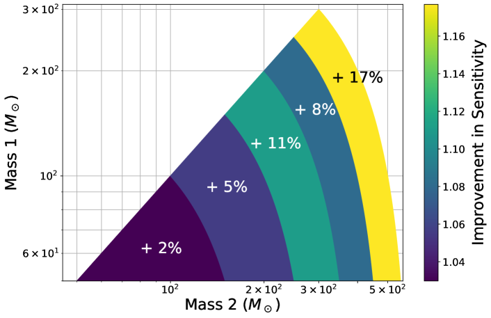
In Fig. 5 we see that the sensitivity of the search has been increased by the addition of the new test, with an increase in sensitivity of for signals with total masses in the range , increasing to for signals with total masses in the range . This is due to the higher rate of glitches matching high mass templates, any decrease in the glitch population will therefore have a larger effect for these templates.
VI Conclusion and Outlook
In this work we have demonstrated a new framework to automatically train complex new signal-consistency tests within modelled searches for gravitational wave signals. We have applied this to the example of a search for IMBH signals, where glitches have a strong effect on the sensitivity of the search. Our framework is able to train a new model, which provides an improved separation of the signal and noise populations allowing the noise triggers to be down-weighted. Using this new test improves the sensitivity of the search to real signals by for signals with total masses in the range and for signals with total masses in the range
The introduction of new tests is difficult and usually requires empirical tuning by hand to be effective, and often requires re-tuning for different target parameter spaces or noise populations. As signal-consistency tests become more complex this can become unfeasible. However, by utilising machine-learning techniques we have shown that we can tune these automatically, removing the burden in improving and optimally tuning these tests. The method we demonstrate here could be applied to any of the commonly used matched-filter search pipelines targeting compact binary mergers.
The population of glitches within the interferometer data continues to be one of the largest challenges facing gravitational wave searches. By continuing to develop signal-consistency tests that specifically target such noise we can continue to improve the sensitivity of searches and increase the chance of observing new events in areas of the parameter space most affected by glitches.
Acknowledgements.
CM was supported by the Science and Technology Facilities Council through the DISCnet Centre for Doctoral Training. IH was supported by STFC grants ST/T000333/1 and ST/V005715/1. This research has made use of data or software obtained from the Gravitational Wave Open Science Center (gw-openscience.org), a service of LIGO Laboratory, the LIGO Scientific Collaboration, the Virgo Collaboration, and KAGRA. LIGO Laboratory and Advanced LIGO are funded by the United States National Science Foundation (NSF) as well as the Science and Technology Facilities Council (STFC) of the United Kingdom, the Max-Planck-Society (MPS), and the State of Niedersachsen/Germany for support of the construction of Advanced LIGO and construction and operation of the GEO600 detector. Additional support for Advanced LIGO was provided by the Australian Research Council. Virgo is funded, through the European Gravitational Observatory (EGO), by the French Centre National de Recherche Scientifique (CNRS), the Italian Istituto Nazionale di Fisica Nucleare (INFN) and the Dutch Nikhef, with contributions by institutions from Belgium, Germany, Greece, Hungary, Ireland, Japan, Monaco, Poland, Portugal, Spain. The construction and operation of KAGRA are funded by Ministry of Education, Culture, Sports, Science and Technology (MEXT), and Japan Society for the Promotion of Science (JSPS), National Research Foundation (NRF) and Ministry of Science and ICT (MSIT) in Korea, Academia Sinica (AS) and the Ministry of Science and Technology (MoST) in Taiwan. For the purpose of open access, the author has applied a CC BY public copyright licence to any Author Accepted Manuscript version arisingReferences
- Abbott et al. [2016a] B. P. Abbott et al. (LIGO Scientific, Virgo), Observation of Gravitational Waves from a Binary Black Hole Merger, Phys. Rev. Lett. 116, 061102 (2016a), arXiv:1602.03837 [gr-qc] .
- Aasi et al. [2015] J. Aasi et al. (LIGO Scientific), Advanced LIGO, Class. Quant. Grav. 32, 074001 (2015), arXiv:1411.4547 [gr-qc] .
- Acernese et al. [2015] F. Acernese et al. (VIRGO), Advanced Virgo: a second-generation interferometric gravitational wave detector, Class. Quant. Grav. 32, 024001 (2015), arXiv:1408.3978 [gr-qc] .
- Akutsu et al. [2021] T. Akutsu et al. (KAGRA), Overview of KAGRA: Detector design and construction history, PTEP 2021, 05A101 (2021), arXiv:2005.05574 [physics.ins-det] .
- Abbott et al. [2018] B. P. Abbott et al. (KAGRA, LIGO Scientific, Virgo, VIRGO), Prospects for observing and localizing gravitational-wave transients with Advanced LIGO, Advanced Virgo and KAGRA, Living Rev. Rel. 21, 3 (2018), arXiv:1304.0670 [gr-qc] .
- Abbott et al. [2021a] R. Abbott et al. (LIGO Scientific, Virgo), GWTC-2: Compact Binary Coalescences Observed by LIGO and Virgo During the First Half of the Third Observing Run, Phys. Rev. X 11, 021053 (2021a), arXiv:2010.14527 [gr-qc] .
- Abbott et al. [2021b] R. Abbott et al. (LIGO Scientific, VIRGO), GWTC-2.1: Deep Extended Catalog of Compact Binary Coalescences Observed by LIGO and Virgo During the First Half of the Third Observing Run, (2021b), arXiv:2108.01045 [gr-qc] .
- Abbott et al. [2021c] R. Abbott et al. (LIGO Scientific, VIRGO, KAGRA), GWTC-3: Compact Binary Coalescences Observed by LIGO and Virgo During the Second Part of the Third Observing Run, (2021c), arXiv:2111.03606 [gr-qc] .
- Nitz et al. [2021a] A. H. Nitz, C. D. Capano, S. Kumar, Y.-F. Wang, S. Kastha, M. Schäfer, R. Dhurkunde, and M. Cabero, 3-OGC: Catalog of Gravitational Waves from Compact-binary Mergers, Astrophys. J. 922, 76 (2021a), arXiv:2105.09151 [astro-ph.HE] .
- Nitz et al. [2021b] A. H. Nitz, S. Kumar, Y.-F. Wang, S. Kastha, S. Wu, M. Schäfer, R. Dhurkunde, and C. D. Capano, 4-OGC: Catalog of gravitational waves from compact-binary mergers, (2021b), arXiv:2112.06878 [astro-ph.HE] .
- Olsen et al. [2022] S. Olsen, T. Venumadhav, J. Mushkin, J. Roulet, B. Zackay, and M. Zaldarriaga, New binary black hole mergers in the LIGO–Virgo O3a data, (2022), arXiv:2201.02252 [astro-ph.HE] .
- Davies et al. [2020] G. S. Davies, T. Dent, M. Tápai, I. Harry, C. McIsaac, and A. H. Nitz, Extending the PyCBC search for gravitational waves from compact binary mergers to a global network, Phys. Rev. D 102, 022004 (2020), arXiv:2002.08291 [astro-ph.HE] .
- Sachdev et al. [2019] S. Sachdev et al., The GstLAL Search Analysis Methods for Compact Binary Mergers in Advanced LIGO’s Second and Advanced Virgo’s First Observing Runs, (2019), arXiv:1901.08580 [gr-qc] .
- Adams et al. [2016] T. Adams, D. Buskulic, V. Germain, G. M. Guidi, F. Marion, M. Montani, B. Mours, F. Piergiovanni, and G. Wang, Low-latency analysis pipeline for compact binary coalescences in the advanced gravitational wave detector era, Class. Quant. Grav. 33, 175012 (2016), arXiv:1512.02864 [gr-qc] .
- Allen et al. [2012] B. Allen, W. G. Anderson, P. R. Brady, D. A. Brown, and J. D. E. Creighton, FINDCHIRP: An Algorithm for detection of gravitational waves from inspiraling compact binaries, Phys. Rev. D 85, 122006 (2012), arXiv:gr-qc/0509116 .
- Babak et al. [2013] S. Babak, R. Biswas, P. R. Brady, D. A. Brown, K. Cannon, C. D. Capano, J. H. Clayton, T. Cokelaer, J. D. E. Creighton, T. Dent, A. Dietz, S. Fairhurst, N. Fotopoulos, G. González, C. Hanna, I. W. Harry, G. Jones, D. Keppel, D. J. A. McKechan, L. Pekowsky, S. Privitera, C. Robinson, A. C. Rodriguez, B. S. Sathyaprakash, A. S. Sengupta, M. Vallisneri, R. Vaulin, and A. J. Weinstein, Searching for gravitational waves from binary coalescence, Phys. Rev. D 87, 024033 (2013).
- Usman et al. [2016] S. A. Usman et al., The PyCBC search for gravitational waves from compact binary coalescence, Class. Quant. Grav. 33, 215004 (2016), arXiv:1508.02357 [gr-qc] .
- Cannon et al. [2012] K. Cannon et al., Toward Early-Warning Detection of Gravitational Waves from Compact Binary Coalescence, Astrophys. J. 748, 136 (2012), arXiv:1107.2665 [astro-ph.IM] .
- Messick et al. [2017] C. Messick, K. Blackburn, P. Brady, P. Brockill, K. Cannon, R. Cariou, S. Caudill, S. J. Chamberlin, J. D. E. Creighton, R. Everett, C. Hanna, D. Keppel, R. N. Lang, T. G. F. Li, D. Meacher, A. Nielsen, C. Pankow, S. Privitera, H. Qi, S. Sachdev, L. Sadeghian, L. Singer, E. G. Thomas, L. Wade, M. Wade, A. Weinstein, and K. Wiesner, Analysis framework for the prompt discovery of compact binary mergers in gravitational-wave data, Phys. Rev. D 95, 042001 (2017).
- Aubin et al. [2021] F. Aubin et al., The MBTA pipeline for detecting compact binary coalescences in the third LIGO–Virgo observing run, Class. Quant. Grav. 38, 095004 (2021), arXiv:2012.11512 [gr-qc] .
- Chu [2017] Q. Chu, Low-latency detection and localization of gravitational waves from compact binary coalescences, Ph.D. thesis, Western Australia U. (2017).
- Venumadhav et al. [2019] T. Venumadhav, B. Zackay, J. Roulet, L. Dai, and M. Zaldarriaga, New search pipeline for compact binary mergers: Results for binary black holes in the first observing run of Advanced LIGO, Phys. Rev. D 100, 023011 (2019), arXiv:1902.10341 [astro-ph.IM] .
- Venumadhav et al. [2020] T. Venumadhav, B. Zackay, J. Roulet, L. Dai, and M. Zaldarriaga, New binary black hole mergers in the second observing run of Advanced LIGO and Advanced Virgo, Phys. Rev. D 101, 083030 (2020), arXiv:1904.07214 [astro-ph.HE] .
- Klimenko et al. [2016] S. Klimenko, G. Vedovato, M. Drago, F. Salemi, V. Tiwari, G. A. Prodi, C. Lazzaro, K. Ackley, S. Tiwari, C. F. Da Silva, and G. Mitselmakher, Method for detection and reconstruction of gravitational wave transients with networks of advanced detectors, Phys. Rev. D 93, 042004 (2016).
- Nuttall [2018] L. K. Nuttall, Characterizing transient noise in the LIGO detectors, Phil. Trans. Roy. Soc. Lond. A 376, 20170286 (2018), arXiv:1804.07592 [astro-ph.IM] .
- Davis et al. [2021] D. Davis et al. (LIGO), LIGO detector characterization in the second and third observing runs, Class. Quant. Grav. 38, 135014 (2021), arXiv:2101.11673 [astro-ph.IM] .
- Allen [2005] B. Allen, time-frequency discriminator for gravitational wave detection, Phys. Rev. D 71, 062001 (2005), arXiv:gr-qc/0405045 .
- Nitz [2018] A. H. Nitz, Distinguishing short duration noise transients in LIGO data to improve the PyCBC search for gravitational waves from high mass binary black hole mergers, Class. Quant. Grav. 35, 035016 (2018), arXiv:1709.08974 [gr-qc] .
- Nitz et al. [2017] A. H. Nitz, T. Dent, T. Dal Canton, S. Fairhurst, and D. A. Brown, Detecting binary compact-object mergers with gravitational waves: Understanding and Improving the sensitivity of the PyCBC search, Astrophys. J. 849, 118 (2017), arXiv:1705.01513 [gr-qc] .
- Chandra et al. [2021] K. Chandra, V. Villa-Ortega, T. Dent, C. McIsaac, A. Pai, I. W. Harry, Cabourn Davies, G. S., and K. Soni, An optimized PyCBC search for gravitational waves from intermediate-mass black hole mergers, Phys. Rev. D 104, 042004 (2021), arXiv:2106.00193 [gr-qc] .
- George and Huerta [2018a] D. George and E. A. Huerta, Deep Neural Networks to Enable Real-time Multimessenger Astrophysics, Phys. Rev. D 97, 044039 (2018a), arXiv:1701.00008 [astro-ph.IM] .
- George and Huerta [2018b] D. George and E. A. Huerta, Deep Learning for Real-time Gravitational Wave Detection and Parameter Estimation: Results with Advanced LIGO Data, Phys. Lett. B 778, 64 (2018b), arXiv:1711.03121 [gr-qc] .
- Gabbard et al. [2018] H. Gabbard, M. Williams, F. Hayes, and C. Messenger, Matching matched filtering with deep networks for gravitational-wave astronomy, Phys. Rev. Lett. 120, 141103 (2018), arXiv:1712.06041 [astro-ph.IM] .
- Gebhard et al. [2019] T. D. Gebhard, N. Kilbertus, I. Harry, and B. Schölkopf, Convolutional neural networks: a magic bullet for gravitational-wave detection?, Phys. Rev. D 100, 063015 (2019), arXiv:1904.08693 [astro-ph.IM] .
- Yan et al. [2022] J. Yan, M. Avagyan, R. E. Colgan, D. Veske, I. Bartos, J. Wright, Z. Márka, and S. Márka, Generalized approach to matched filtering using neural networks, Phys. Rev. D 105, 043006 (2022), arXiv:2104.03961 [astro-ph.IM] .
- Wei and Huerta [2021] W. Wei and E. A. Huerta, Deep learning for gravitational wave forecasting of neutron star mergers, Phys. Lett. B 816, 136185 (2021), arXiv:2010.09751 [gr-qc] .
- Wei et al. [2021a] W. Wei, E. A. Huerta, M. Yun, N. Loutrel, M. A. Shaikh, P. Kumar, R. Haas, and V. Kindratenko, Deep Learning with Quantized Neural Networks for Gravitational-wave Forecasting of Eccentric Compact Binary Coalescence, Astrophys. J. 919, 82 (2021a), arXiv:2012.03963 [gr-qc] .
- Wei et al. [2021b] W. Wei, A. Khan, E. A. Huerta, X. Huang, and M. Tian, Deep Learning Ensemble for Real-time Gravitational Wave Detection of Spinning Binary Black Hole Mergers, Phys. Lett. B 812, 136029 (2021b), arXiv:2010.15845 [gr-qc] .
- Schäfer et al. [2020] M. B. Schäfer, F. Ohme, and A. H. Nitz, Detection of gravitational-wave signals from binary neutron star mergers using machine learning, Phys. Rev. D 102, 063015 (2020), arXiv:2006.01509 [astro-ph.HE] .
- Krastev [2020] P. G. Krastev, Real-Time Detection of Gravitational Waves from Binary Neutron Stars using Artificial Neural Networks, Phys. Lett. B 803, 135330 (2020), arXiv:1908.03151 [astro-ph.IM] .
- Schäfer and Nitz [2022] M. B. Schäfer and A. H. Nitz, From one to many: A deep learning coincident gravitational-wave search, Phys. Rev. D 105, 043003 (2022), arXiv:2108.10715 [astro-ph.IM] .
- Abadie et al. [2012] J. Abadie et al. (LIGO Scientific, VIRGO), Search for Gravitational Waves from Low Mass Compact Binary Coalescence in LIGO’s Sixth Science Run and Virgo’s Science Runs 2 and 3, Phys. Rev. D 85, 082002 (2012), arXiv:1111.7314 [gr-qc] .
- Abbott et al. [2016b] B. P. Abbott et al. (LIGO Scientific, Virgo), GW150914: First results from the search for binary black hole coalescence with Advanced LIGO, Phys. Rev. D 93, 122003 (2016b), arXiv:1602.03839 [gr-qc] .
- Abbott et al. [2009] B. P. Abbott et al. (LIGO Scientific), Search for Gravitational Waves from Low Mass Binary Coalescences in the First Year of LIGO’s S5 Data, Phys. Rev. D 79, 122001 (2009), arXiv:0901.0302 [gr-qc] .
- Cabero et al. [2019] M. Cabero et al., Blip glitches in Advanced LIGO data, Class. Quant. Grav. 36, 155010 (2019), arXiv:1901.05093 [physics.ins-det] .
- Abadi et al. [2015] M. Abadi, A. Agarwal, P. Barham, E. Brevdo, Z. Chen, C. Citro, G. S. Corrado, A. Davis, J. Dean, M. Devin, S. Ghemawat, I. Goodfellow, A. Harp, G. Irving, M. Isard, Y. Jia, R. Jozefowicz, L. Kaiser, M. Kudlur, J. Levenberg, D. Mané, R. Monga, S. Moore, D. Murray, C. Olah, M. Schuster, J. Shlens, B. Steiner, I. Sutskever, K. Talwar, P. Tucker, V. Vanhoucke, V. Vasudevan, F. Viégas, O. Vinyals, P. Warden, M. Wattenberg, M. Wicke, Y. Yu, and X. Zheng, TensorFlow: Large-scale machine learning on heterogeneous systems (2015), software available from tensorflow.org.
- Developers [2021] T. Developers, Tensorflow (2021), specific TensorFlow versions can be found in the ”Versions” list on the right side of this page. See the full list of authors on GitHub.
- Ruder [2017] S. Ruder, An overview of gradient descent optimization algorithms (2017), arXiv:1609.04747 [cs.LG] .
- LeCun et al. [2015] Y. LeCun, Y. Bengio, and G. Hinton, Deep learning, Nature 521, 436 (2015).
- Harry and Fairhurst [2011] I. W. Harry and S. Fairhurst, A targeted coherent search for gravitational waves from compact binary coalescences, Phys. Rev. D 83, 084002 (2011), arXiv:1012.4939 [gr-qc] .
- Williamson et al. [2014] A. R. Williamson, C. Biwer, S. Fairhurst, I. W. Harry, E. Macdonald, D. Macleod, and V. Predoi, Improved methods for detecting gravitational waves associated with short gamma-ray bursts, Phys. Rev. D 90, 122004 (2014), arXiv:1410.6042 [gr-qc] .
- Vallisneri et al. [2015] M. Vallisneri, J. Kanner, R. Williams, A. Weinstein, and B. Stephens, The LIGO Open Science Center, J. Phys. Conf. Ser. 610, 012021 (2015), arXiv:1410.4839 [gr-qc] .
- Abbott et al. [2021d] R. Abbott et al. (LIGO Scientific, Virgo), Open data from the first and second observing runs of Advanced LIGO and Advanced Virgo, SoftwareX 13, 100658 (2021d), arXiv:1912.11716 [gr-qc] .
- Taracchini et al. [2014] A. Taracchini, A. Buonanno, Y. Pan, T. Hinderer, M. Boyle, D. A. Hemberger, L. E. Kidder, G. Lovelace, A. H. Mroué, H. P. Pfeiffer, M. A. Scheel, B. Szilágyi, N. W. Taylor, and A. Zenginoglu, Effective-one-body model for black-hole binaries with generic mass ratios and spins, Phys. Rev. D 89, 061502(R) (2014).
- Bohé et al. [2017] A. Bohé, L. Shao, A. Taracchini, A. Buonanno, S. Babak, I. W. Harry, I. Hinder, S. Ossokine, M. Pürrer, V. Raymond, T. Chu, H. Fong, P. Kumar, H. P. Pfeiffer, M. Boyle, D. A. Hemberger, L. E. Kidder, G. Lovelace, M. A. Scheel, and B. Szilágyi, Improved effective-one-body model of spinning, nonprecessing binary black holes for the era of gravitational-wave astrophysics with advanced detectors, Phys. Rev. D 95, 044028 (2017).
- Varma et al. [2019] V. Varma, S. E. Field, M. A. Scheel, J. Blackman, D. Gerosa, L. C. Stein, L. E. Kidder, and H. P. Pfeiffer, Surrogate models for precessing binary black hole simulations with unequal masses, Phys. Rev. Research. 1, 033015 (2019), arXiv:1905.09300 [gr-qc] .
- Cotesta et al. [2018] R. Cotesta, A. Buonanno, A. Bohé, A. Taracchini, I. Hinder, and S. Ossokine, Enriching the Symphony of Gravitational Waves from Binary Black Holes by Tuning Higher Harmonics, Phys. Rev. D 98, 084028 (2018), arXiv:1803.10701 [gr-qc] .
- Cotesta et al. [2020] R. Cotesta, S. Marsat, and M. Pürrer, Frequency domain reduced order model of aligned-spin effective-one-body waveforms with higher-order modes, Phys. Rev. D 101, 124040 (2020), arXiv:2003.12079 [gr-qc] .
- Nesterov [1983] Y. Nesterov, A method for solving the convex programming problem with convergence rate , Proceedings of the USSR Academy of Sciences 269, 543 (1983).