gwadaptive_scattering: an automated pipeline for scattered light noise characterization

Abstract

Scattered light noise affects the sensitivity of gravitational waves detectors. The characterization of such noise is needed to mitigate it. The time-varying filter empirical mode decomposition algorithm is suitable for identifying signals with time-dependent frequency such as scattered light noise (or scattering). We present a fully automated pipeline based on the pytvfemd library, a python implementation of the tvf-EMD algorithm, to identify objects inducing scattering in the gravitational-wave channel with their motion. The pipeline application to LIGO Livingston O3 data shows that most scattering noise is due to the penultimate mass at the end of the X-arm of the detector (EXPUM) and with a motion in the micro-seismic frequency range.

1 Introduction

Advanced LIGO [1] and Advanced Virgo [2] are gravitational-wave detectors, instruments designed to measure tiny spacetime distortions called gravitational waves. These extreme-sensitive instruments are capable of detecting strain amplitudes smaller than ${10}^{-23}$ $\mathrm{/}\sqrt{\text{\mathrm{ Hz }}}$ and have observed gravitational waves from distinct systems such as binary black holes, binary neutron stars, and neutron star - black hole [3, 4, 5]. However, such sensitivity can be overwhelmed by intrinsic noises or local environment noises coupling into the instrument [6, 7, 8]. One common noise affecting the sensitivity of gravitational-wave detectors is scattered-light noise [9]. It originates when a fraction of laser light is undesirably scattered, reflected from moving surfaces, and recombined in any of the detectors’ optical cavities [10]. Scattered-light noise (or scattering) manifests as arches in the detector’s output with a frequency given by:

$$f_{\text{arch}}(t)=\frac{2N}{\lambda}|v_{\text{surface}}(t)|$$ (1)

Where $\lambda$ is the laser wavelength, $v_{\text{surface}}$ is the velocity at which the scattering surface is moving, and $N$ is the number of times the perturbed surface reflects the light before it recombines with the laser beam again. Studies had been made to locate and mitigate scattering in LIGO [11, 12]. These methods have employed the Hilbert-Huang transform [13], a technique for analyzing nonlinear and non-stationary data, consisting of utilizing empirical mode decomposition (EMD) and the Hilbert transform. In Virgo, the time-varying filter EMD (tvf-EMD) [14] adaptive algorithm was used to improve the scattering’s origin localization [15] and to denoise environmental signals [16]. Posteriorly, the scattering characterization, e.g., identifying the reflective surface motion frequency, is necessary to understand how the noise originated. For scattered light characterization, we used pytvfemd, a Python library that implements tvf-EMD [17]. We show results from the application of the tool on data recorded by the LIGO Livingston detector (LLO) during the third observing run (so called O3). We discuss which areas of the detector and frequencies had a high correlation with the scattering, based on the adopted methodology. Finally, we present gwadaptive_scattering, a new fully automated pipeline based on tvf-EMD to locate and characterize the origin of scattered light glitches as obtained from GravitySpy, a machine learning image recognition tool that classifies transient noise instances (also called triggers) in the strain data [18]

2 Methodology

2.1 Time-varying filter EMD and pytvfemd

EMD is a method to empirically break down any nonlinear, non-stationary data set into a finite number of intrinsic mode functions (IMF) through a sifting process. Ideally, each IMF will include a narrow band of oscillations, in order for Hilbert spectral analysis to give meaningful results. Still, EMD fails to distinguish components whose frequencies are too similar [19]. Also, noisy data could lead to mode mixed IMFs, meaning that the IMF extracted by EMD might contain oscillations of widely different scales or that multiple IMFs contain the same oscillatory mode [20]. A mode mixed IMF typically has no physical meaning. The time-varying filter EMD mitigates mode mixing and improves the IMFs frequency resolution, replacing the known IMF concept with the local narrow-band oscillatory modes. The tvf-EMD employs a B-spline [21] as the time-varying filter to extract these local narrow-band modes. Furthermore, the algorithm’s sifting process stops when the ratio between the Loughlin instantaneous bandwidth $B_{\text{Loughlin}}(t)$ and the weighted average of the instantaneous frequencies $\varphi_{\text{average}}(t)$ is lower than a selected threshold $\xi$. The definition of $B_{\text{Loughlin}}(t)$, $\varphi_{\text{average}}(t)$, and a full description of the algorithm can be found in [14]. Regarding tvf-EMD, the relevant parameters to consider are the bandwitdth threshold ratio $\xi$ and the B-spline order $n$. While $\xi$ determines the threshold on the bandwidth of the extracted modes to stop the sifting process, $n$ is related to the time varying filter frequency roll off. Following [14], these parameters were set to $\xi=0.1$ and $n=26$. pytvfemd [17] is a Python package that implements the tvf-EMD algorithm based on an existing MATLAB code [22]. In this paper it was used for scattering characterization, but it is also available for the analysis of other non linear and non stationary data. The main function tvfemd takes the signal as input and returns its intrinsic mode functions. Other inputs are the algorithm’s main parameters (i.e., $\xi$ and $n$) and the number of IMFs to be extracted.

2.2 Scattering characterization pipeline

The pipeline follows the same procedure described in [11], except that instead of EMD, we use tvf-EMD for the sifting process, as implemented in [15]. The pipeline completes the following steps to locate the origin of scattering noise and characterize it:

1. Identify times when the data is affected by scattering, using the times and peak frequencies of the scattering arches provided by GravitySpy.

2. Lowpass filter the data using the peak frequency as a cutoff.

3. Get the scattering’s instantaneous amplitude IA, using tvf-EMD and the Hilbert transform.

4. Generate the scattering predictors for a given list of auxiliary sensors, using Equation 1.

5. Estimate the Pearson correlation coefficient $\rho$ between the instantaneous amplitude and the predictors. We consider only the first IMF for each channel, as it is the one relevant after the lowpass filter. We call culprit the predictor with the highest correlation.

6. Estimate the associated frequency to the scattering using the culprit’s motion frequency. We calculated this frequency by looking for the highest peak in the amplitude spectrum of the culprit’s motion data.

Steps 1 and 6 are an addition to this new version of the pipeline. For Step 4, we use $N=1$ to calculate the scattering predictors because the correlation in Step 5 ignores the signals’ amplitude. We use data from the third observing run (O3) for our analyses. O3 began in April 2019 and lasted nearly one year, with a month-long commissioning break in October 2019. The periods before and after the break are known as O3a and O3b, respectively. In January 2020, scattering noise decreased after commissioners reduced the relative motion between the test mass and the reaction mass –see section 6 in [12]. This noise reduction using the suspensions control system is known as RC tracking. We identify these periods before and after the RC tracking implementation as O3b1 and O3b2.

We select the triggers classified as scattered_light by GravitySpy, with a confidence greater than 0.9 and SNR greater than 10. There are $3706$, $24566$, and $8623$ triggers in LIGO Livingston data with these characteristics in O3a, O3b1, and O3b2, respectively, after removing triggers with duplicated GPS time. Table 1 summarizes the scattering triggers of the study.

Table 1: Data employed in this study. Scattering triggers with confidence greater than 0.9 and SNR greater than 10, during O3 in LIGO Livingston.

Epoch	Starting date	Ending date	Description	Scattering triggers
O3a	Apr 01, 2019	Sep 30, 2019	O3 first part	$3706$
Comm	Oct 01, 2019	Oct 31, 2019	O3 commissioning break	NA
O3b1	Nov 01, 2019	Jan 06, 2020	O3 second part before RC tracking	$24566$
O3b2	Jan 07, 2020	Mar 27, 2020	O3 second part after RC tracking	$8623$

LIGO samples the gravitational-wave channel data (so-called DARM-Differential Arm Motion), with a frequency of 16384 $\mathrm{Hz}$, and auxiliary data such as the position of the detector’s mirrors at lower rates. We use 60 $\mathrm{s}$ of DARM and auxiliary data around the peak time of each scattering trigger and downsampled at 256 $\mathrm{Hz}$. Besides the gravitational-wave channel, the LIGO detectors record over 200000 auxiliary sensors (or channels) that monitor instrument behavior and environmental conditions. We use a short list of channels monitoring the optics’ suspension system top stage motion for our study, including the channel monitoring the end X-arm penultimate stage motion. We use DARM and auxiliary channels to calculate the scattering instantaneous amplitude and the scattering predictors, respectively. In Appendix A, we list the name of these channels, including a short description. In Appendix B, we include a LIGO configuration schematic to visualize the location of its optics better. A list of abbreviations and acronyms can be consulted in [23].

3 Results

3.1 Validation

We tested the tool on data dominated by scattering noise previously identified to be correlated with the motion of penultimate mass at the end of the X arm of the detector (EXPUM) [24], with starting time December 12, 2019 20:56:40 (GPS 1260219418). We used the list of channels in Table 3, and the tool pointed EXPUM as the culprit with $\rho=$ 0.77. Other end X-arm predictors had correlations $\rho<0.73$. In contrast, predictors unrelated to the end X-arm had correlations $\rho<0.39$. Figure 1 shows the culprit, i.e. the EXPUM predictor, overlapping with the DARM instantaneous amplitude (left graph) and spectrogram (right graph), validating the performance of our tool. We generated the EXPUM predictor, 40 $\mathrm{s}$ around GPS 1260219438, with $N=3$ for better overlapping visualization.

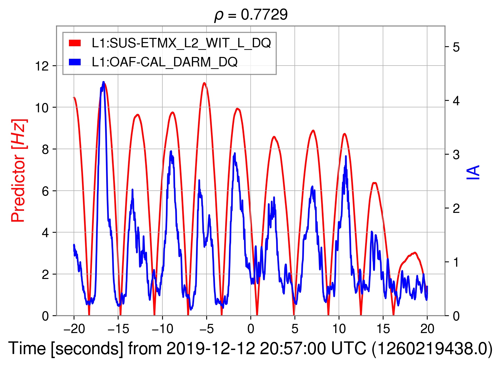
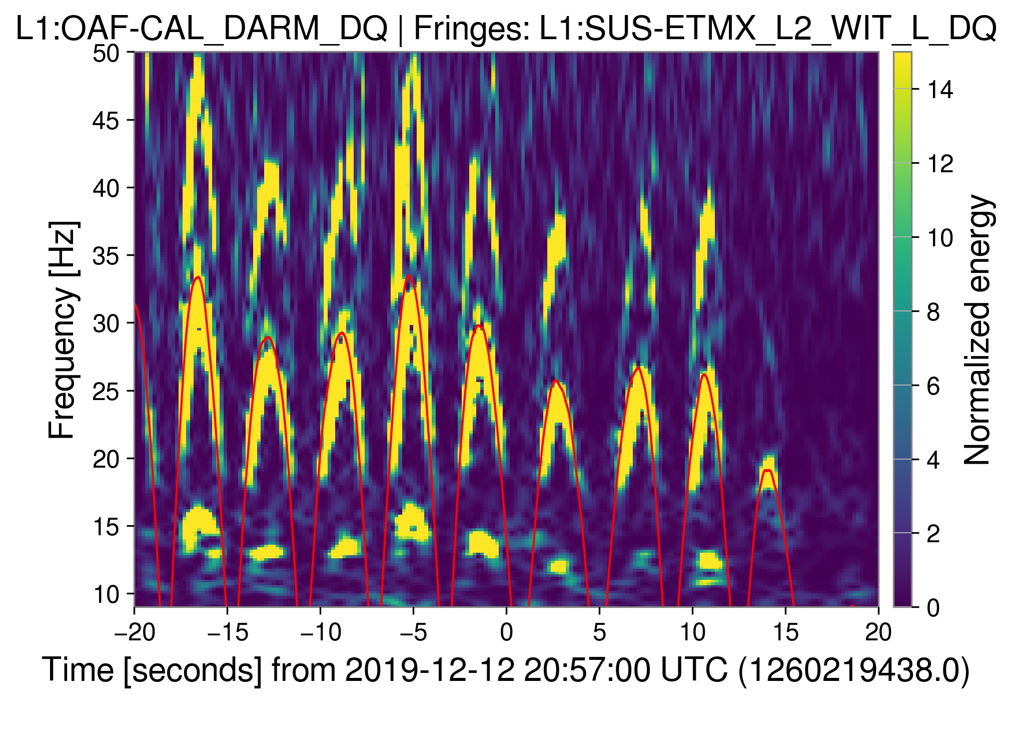
Figure 1: Instantaneous amplitude (left plot) and spectrogram (right plot) of DARM data dominated by scattering noise and the scattering culprit (red line). In this validation example, the culprit is associated with the end X-arm penultimate mass (EXPUM). We used $N=3$ to generate the EXPUM scattering predictor for better visualization of the overlapping.

3.2 Scattering associated to X-arm end mass

The implementation of RC tracking between O3b1 and O3b2 lead to a reduction of scattered light glitches due to the reaction mass [12]. With our method, we also found a reduction in the percentage of scattered light glitches for which the obtained culprit is EXPUM, with $\rho>0.5$, between O3b1 and O3b2.

We grouped the associated frequency to the scattering in the bands defined in Table 2. We also found that the percentage of EXPUM scattering associated with the frequency band B decreased in O3b2. Our results support those in [12], where they found that a major part of the scattering was associated with the 0.1 $\mathrm{Hz}$–0.3 $\mathrm{Hz}$ band (so-called micro-seismic band) and was reduced after the RC tracking implementation.

Table 2: Correspondence between frequency bands values and labels.

Label	Frequency band [$\mathrm{Hz}$]	Label	Frequency band [$\mathrm{Hz}$]
A	0.03–0.10	D	1.00–3.00
B	0.10–0.30	E	3.00–10.0
C	0.30–1.00	ELSE	$<$ 0.03, $\geq$ 10.0

Figure 2 shows that the percentage of EXPUM scattering decreased from 15.2% in O3b1 to 1.4% in O3b2 (left plot) and the EXPUM scattering associated with the micro-seismic band decreased from 14% in O3b1 to 1% in O3b2 (right plot).

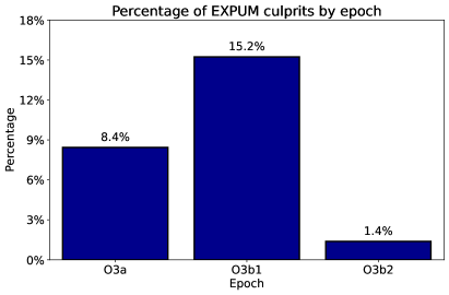
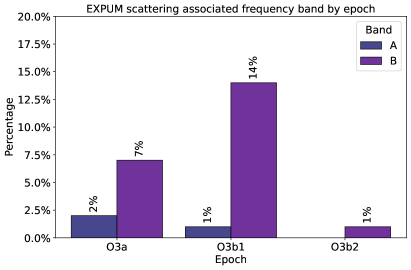
Figure 2: Left plot - Percentage of scattering in LIGO Livingston associated with EXPUM during O3. Right plot - Percentage of scattering in LIGO Livingston associated with EXPUM and the frequency bands A (0.03 $\mathrm{Hz}$–0.1 $\mathrm{Hz}$) and B (0.1 $\mathrm{Hz}$–0.3 $\mathrm{Hz}$) during O3. Our tool quantified the reduction of this scattering after commissioning improvements.

3.3 O3 scattering

We extended the study to investigate the scattering origin and associated frequency based on location within the detector. Consult Figure 5 for better comprehension of the distinct vacuum chamber locations.

We found that most of the O3 scattering in LIGO Livingston was linked to BSC4, the vacuum chamber enclosing the X-arm end test mass, and therefore EXPUM. When grouped by the scattering associated frequency, we observed a reduction in the band B scattering, from 93.3% in O3b1 to 76.9% in O3b2. We saw a reduction of scattering in band A in O3b2 with respect to O3a, but an increase with respect to O3b1. Figure 3 shows the ranking of O3 scattering by location in the detector (left plot) and the percentage of scattering associated with the frequency bands by epoch (right plot).

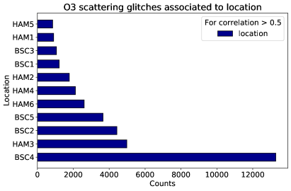
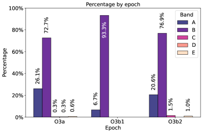
Figure 3: Left plot - Ranking of O3 scattering by location in the detector. Right plot - Percentage of scattering associated with the distinct frequency bands in Table 2 during O3. We omit the columns with a value equals to 0.

4 Daily-basis automated pipeline

We present gwadaptive_scattering, a Python package that builds the automated pipeline for the scattering localization and characterization on the LIGO computers. The pipeline generates three main files for HTCondor [25], a high-throughput computing software for distributed parallelization of tasks to accelerate the process for a given target channel (i.e., the scattering witness channel), and GPS times list. The first file completes the steps describes in Section 2.2. We called these the analysis jobs. The second file merges the analysis jobs results in a single data frame. We denominate these the summary jobs. The third file organizes the hierarchy, running the analysis jobs first and then the summary jobs. A screenshot of the summary jobs data frame is shown in Figure 4 and includes the following columns:

• GPS: GPS time (from GravitySpy).

• Frequency: Glitch peak frequency (from GravitySpy).

• SNR: Glitch signal-to-noise ratio (from GravitySpy).

• Epoch: O3a, O3b1, O3b2.

• Culprit: Name of channel with highest correlation. For possible values see Table 3.

• Correlation: Correlation coefficient between scattering and culprit.

• Mean frequency: Culprit’s mean frequency calculated as the highest peak in its spectrum.

• Range: Ground motion frequency bands used in LIGO. Possible values are A, B, C, D, E, and ELSE (see Table 2).

• Location: Chamber containing the optic (see Table 3).

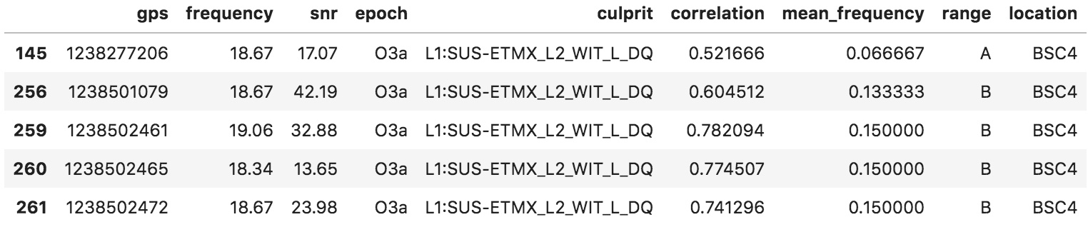
Figure 4: Screenshot of the results data frame generated by our gwadaptive_scattering pipeline.

Additionally, the pipeline creates a directory containing the results and the plots and presents them in an HTML page format.

5 Conclusions

We have presented an automated pipeline based on the tvf-EMD algorithm to identify and characterize scattered light noise in data recorded by the LIGO Livingston gravitational-wave detector in its third observing run, O3.

We found the correlation between the LIGO Livingston scattering noise, the motion of the penultimate mass at the end of the detector’s X-arm, and the micro-seismic frequency band (0.1 $\mathrm{Hz}$–0.3 $\mathrm{Hz}$) was high; a similar result previously discovered by other means. We used our tool to quantify the percentage of scattering by location and frequency. We found that most of the scattering was linked to the chamber enclosing the X-arm end mass, and the micro-seismic frequency scattering decreased after the commissioning improvements known as RC tracking.

In upcoming observing runs, this tool can be used in other detectors such as LIGO Hanford and Virgo. Its results could be presented in summary pages for rapid consultation aimed to help commissioners. The long-term analysis of the pipeline results will lead to a better characterization of the detectors.

The gwadaptive_scattering pipeline proved to be useful in identifying and characterizing time- and frequency-varying features in data of large-scale gravitational-wave detectors. The adaptive nature of the tvf-emd algorithm to nonlinear and non-stationary data suggests that our tool could be employed to identify and characterize another type of noise in gravitational-wave astronomy or other fields.

Appendix A Channel names

Table 3: List of channels of investigated objects, including 23 mirrors, 4 reaction masses (CPX, CPY, ERMX, ERMY), and 2 transmission monitors (TMSX, TMSY). Where L refers to the longitudinal directions.

Short	Channel	Chamber	Description
Name
DARM	L1:OAF-CAL_DARM_DQ	NA	Gravitational-wave channel
BS	L1:SUS-BS_M2_WIT_L_DQ	BSC2	Beam Splitter
MC1	L1:SUS-MC1_M1_DAMP_L_IN1_DQ	HAM2	Mode Cleaner optic 1
MC2	L1:SUS-MC2_M1_DAMP_L_IN1_DQ	HAM3	Mode Cleaner optic 2
MC3	L1:SUS-MC3_M1_DAMP_L_IN1_DQ	HAM2	Mode Cleaner optic 3
PRM	L1:SUS-PRM_M1_DAMP_L_IN1_DQ	HAM2	Power Recycling Mirror
PR2	L1:SUS-PR2_M1_DAMP_L_IN1_DQ	HAM3	Power Recycling optic 2
PR3	L1:SUS-PR3_M1_DAMP_L_IN1_DQ	HAM2	Power Recycling optic 3
SRM	L1:SUS-SRM_M1_DAMP_L_IN1_DQ	HAM5	Signal Recycling Mirror
SR2	L1:SUS-SR2_M1_DAMP_L_IN1_DQ	HAM4	Signal Recycling optic 2
SR3	L1:SUS-SR3_M1_DAMP_L_IN1_DQ	HAM5	Signal Recycling optic 3
RM1	L1:SUS-RM1_M1_DAMP_L_IN1_DQ	HAM1	Recycling Mirror 1
RM2	L1:SUS-RM2_M1_DAMP_L_IN1_DQ	HAM1	Recycling Mirror 2
IM1	L1:SUS-IM1_M1_DAMP_L_IN1_DQ	HAM2	Input Mirror 1
IM2	L1:SUS-IM2_M1_DAMP_L_IN1_DQ	HAM2	Input Mirror 2
IM3	L1:SUS-IM3_M1_DAMP_L_IN1_DQ	HAM2	Input Mirror 3
IM4	L1:SUS-IM4_M1_DAMP_L_IN1_DQ	HAM2	Input Mirror 4
OM1	L1:SUS-OM1_M1_DAMP_L_IN1_DQ	HAM6	Output Mirror 1
OM2	L1:SUS-OM2_M1_DAMP_L_IN1_DQ	HAM6	Output Mirror 2
OM3	L1:SUS-OM3_M1_DAMP_L_IN1_DQ	HAM6	Output Mirror 3
TMSX	L1:SUS-TMSX_M1_DAMP_L_IN1_DQ	BSC4	Transmission Monitor
			Suspension in X-arm
TMSY	L1:SUS-TMSY_M1_DAMP_L_IN1_DQ	BSC5	Transmission Monitor
			Suspension in Y-arm
EXPUM	L1:SUS-ETMX_L2_WIT_L_DQ	BSC4	End X-arm Penultimate Mass

Appendix B Seismic Isolation and Suspensions Layout of Advanced LIGO

Figure 5: Schematic of the Advanced LIGO optical layout [26] showing the laser beam path through optics, which are suspended via many different types and different number of layers of seismic isolation. BSC chambers house the core interferometer optics: the beam splitter, two sets of “input” and “end” test masses that comprise each Fabry-Perot arm cavity. These test mass quadruple pendula (QUAD) contain two parallel suspension chains, one for the test mass itself, and one for a “reaction chain” where each stage is used for quiet actuation of the corresponding stage of the main chain. The transmission monitor and telescope suspension (TMTS) holds optics used for arm cavity power monitoring and angular displacement sensing during observation and arm length stabilization during lock acquisition. HAM chambers house auxiliary optics and platforms used for power recycling, signal recycling, beam expanding or reducing telescopes, mode cleaning, beam steering, supporting the squeezed light system, and suspending the differential arm length readout used for gravitational wave detection. For a review of these systems, see for example [27], and references therein.

References

- [1] J. Aasi et al., “Advanced LIGO,” Class. Quant. Grav., vol. 32, p. 074001, 2015.
- [2] F. Acernese, T. Adams, K. Agatsuma, L. Aiello, A. Allocca, A. Amato, S. Antier, N. Arnaud, S. Ascenzi, P. Astone, et al., “Status of the Advanced Virgo gravitational wave detector,” International Journal of Modern Physics A, vol. 32, no. 28n29, p. 1744003, 2017.
- [3] B. P. Abbott et al., “GWTC-1: A Gravitational-Wave Transient Catalog of Compact Binary Mergers Observed by LIGO and Virgo during the First and Second Observing Runs,” Phys. Rev. X, vol. 9, no. 3, p. 031040, 2019.
- [4] R. Abbott et al., “GWTC-2: Compact binary coalescences observed by LIGO and Virgo during the first half of the third observing run,” Phys. Rev. X, vol. 11, no. 2, p. 021053, 2021.
- [5] R. Abbott et al., “Observation of Gravitational Waves from Two Neutron Star–Black Hole Coalescences,” Astrophys. J. Lett., vol. 915, no. 1, p. L5, 2021.
- [6] B. P. Abbott et al., “Characterization of transient noise in Advanced LIGO relevant to gravitational wave signal GW150914,” Class. Quant. Grav., vol. 33, no. 13, p. 134001, 2016.
- [7] L. Nuttall, “Characterizing transient noise in the LIGO detectors,” Philosophical Transactions of the Royal Society A: Mathematical, Physical and Engineering Sciences, vol. 376, no. 2120, p. 20170286, 2018.
- [8] D. Davis, J. S. Areeda, B. K. Berger, R. Bruntz, A. Effler, R. C. Essick, R. P. Fisher, P. Godwin, E. Goetz, A. F. Helmling-Cornell, et al., “LIGO detector characterization in the second and third observing runs,” Class. Quant. Grav., vol. 38, no. 13, p. 135014, 2021.
- [9] S. Soni et al., “Discovering features in gravitational-wave data through detector characterization, citizen science and machine learning,” 3 2021.
- [10] T. Accadia et al., “Noise from scattered light in Virgo’s second science run data,” Class. Quant. Grav., vol. 27, p. 194011, 2010.
- [11] G. Valdes, B. O’Reilly, and M. Diaz, “A Hilbert–Huang transform method for scattering identification in LIGO,” Class. Quant. Grav., vol. 34, no. 23, p. 235009, 2017.
- [12] S. Soni et al., “Reducing scattered light in LIGO’s third observing run,” Class. Quant. Grav., vol. 38, no. 2, p. 025016, 2020.
- [13] N. E. Huang, Z. Shen, S. R. Long, M. C. Wu, H. H. Shih, Q. Zheng, N. C. Yen, C. C. Tung, and H. H. Liu, “The empirical mode decomposition and the Hilbert spectrum for nonlinear and non-stationary time series analysis,” Proceedings of the Royal Society of London Series A, vol. 454, pp. 903–998, March 1998.
- [14] H. Li, Z. Li, and W. Mo, “A time varying filter approach for empirical mode decomposition,” Signal Processing, vol. 138, 03 2017.
- [15] A. Longo, S. Bianchi, W. Plastino, N. Arnaud, A. Chiummo, I. Fiori, B. Swinkels, and M. Was, “Scattered light noise characterisation at the Virgo interferometer with tvf-EMD adaptive algorithm,” Class. Quant. Grav., vol. 37, no. 14, p. 145011, 2020.
- [16] A. Longo, S. Bianchi, W. Plastino, I. Fiori, D. Fiorucci, J. Harms, F. Paoletti, M. Barsuglia, and M. Falxa, “Adaptive Denoising of Acoustic Noise Injections Performed at the Virgo Interferometer,” Pure Appl. Geophys., vol. 177, no. 7, pp. 3395–3406, 2020.
- [17] S. Bianchi, “stfbnc/pytvfemd v0.1,” Zenodo, February 2021. https://doi.org/10.5281/zenodo.4568706.
- [18] M. Zevin et al., “Gravity Spy: Integrating Advanced LIGO Detector Characterization, Machine Learning, and Citizen Science,” Class. Quant. Grav., vol. 34, no. 6, p. 064003, 2017.
- [19] G. Rilling and P. Flandrin, “One or two frequencies? the empirical mode decomposition answers,” IEEE Transactions on Signal Processing, vol. 56, no. 1, pp. 85–95, 2008.
- [20] N. E. Huang, Z. Shen, and S. R. Long, “A new view of nonlinear water waves: The Hilbert spectrum,” Annual Review of Fluid Mechanics, vol. 31, no. 1, pp. 417–457, 1999.
- [21] M. Unser, “Splines: a perfect fit for signal and image processing,” IEEE Signal Processing Magazine, vol. 16, no. 6, pp. 22–38, 1999.
- [22] S. Li, “Time varying filter based empirical mode decomposition (tvf-emd),” MATLAB Central File Exchange, 2021.
- [23] D. Shoemaker et al., “LIGO - Virgo - KAGRA (LVK) Abbreviations and Acronyms List.” LIGO-Document-M080375, 2020. https://dcc.ligo.org/LIGO-M080375/public.
- [24] R. Schofield, “aLIGO LHO Logbook.” 54298, 2020.
- [25] B. Bockelman, T. Cartwright, J. Frey, E. M. Fajardo, B. Lin, M. Selmeci, T. Tannenbaum, and M. Zvada, “Commissioning the HTCondor-CE for the open science grid,” Journal of Physics: Conference Series, vol. 664, p. 062003, December 2015.
- [26] J. Kissel, “aLIGO Seismic Isolation and Suspensions cartoon.” LIGO-Document-G1200071, 2017. https://dcc.ligo.org/LIGO-G1200071/public.
- [27] F. Matichard, D. Martynov, B. Shapiro, J. Rollins, and D. Coyne, “An overview of the control layers in ligo 4km interferometers,” in Proceedings-ASPE 2016 Spring Topical Meeting: Precision Mechatronic System Design and Control, pp. 17–22, 2016.