LIGO Detector Characterization in the Second and Third Observing Runs

D Davis¹, J S Areeda², B K Berger³, R Bruntz⁴, A Effler⁵, R C Essick⁶, R P Fisher⁴, P Godwin⁷, E Goetz^8,9,10, A F Helmling-Cornell¹¹, B Hughey¹², E Katsavounidis¹³, A P Lundgren¹⁴, D M Macleod¹⁵, Z Márka¹⁶, T J Massinger¹³, A Matas¹⁷, J McIver⁸, G Mo¹³, K Mogushi⁹, P Nguyen¹¹, L K Nuttall¹⁴, R M S Schofield¹¹, D H Shoemaker¹³, S Soni¹⁰, A L Stuver¹⁸, A L Urban¹⁰, G Valdes¹⁰, M Walker⁴, R Abbott¹, C Adams⁵, R X Adhikari¹, A Ananyeva¹, S Appert¹, K Arai¹, Y Asali¹⁶, S M Aston⁵, C Austin¹⁰, A M Baer⁴, M Ball¹¹, S W Ballmer¹⁹, S Banagiri²⁰, D Barker²¹, C Barschaw²², L Barsotti¹³, J Bartlett²¹, J Betzwieser⁵, R Beda⁸, D Bhattacharjee⁹, J Bidler², G Billingsley¹, S Biscans^13,1, C D Blair⁵, R M Blair²¹, N Bode^23,24, P Booker^23,24, R Bork¹, A Bramley⁵, A F Brooks¹, D D Brown²⁵, A Buikema¹³, C Cahillane¹, T A Callister^26,27, G Caneva Santoro^28,29, K C Cannon³⁰, J Carlin³¹, K Chandra³², X Chen³³, N Christensen³⁴, A A Ciobanu²⁵, F Clara²¹, C M Compton²¹, S J Cooper³⁵, K R Corley¹⁶, M W Coughlin²⁰, S T Countryman¹⁶, P B Covas³⁶, D C Coyne¹, S G Crowder³⁷, T Dal Canton^17,38, B Danila³⁹, L E H Datrier⁴⁰, G S Davies^41,14, T Dent⁴¹, N A Didio¹⁹, C Di Fronzo³⁵, K L Dooley^15,42, J C Driggers²¹, P Dupej⁴⁰, S E Dwyer²¹, T Etzel¹, M Evans¹³, T M Evans⁵, S Fairhurst¹⁵, J Feicht¹, A Fernandez-Galiana¹³, R Frey¹¹, P Fritschel¹³, V V Frolov⁵, P Fulda⁴³, M Fyffe⁵, B U Gadre¹⁷, J A Giaime^10,5, K D Giardina⁵, G González¹⁰, S Gras¹³, C Gray²¹, R Gray⁴⁰, A C Green⁴³, A Gupta¹, E K Gustafson¹, R Gustafson⁴⁴, J Hanks²¹, J Hanson⁵, T Hardwick¹⁰, I W Harry¹⁴, R K Hasskew⁵, M C Heintze⁵, J Heinzel³⁴, N A Holland⁴⁵, I J Hollows⁴⁶, C G Hoy¹⁵, S Hughey²², S P Jadhav⁴⁷, K Janssens⁴⁸, G Johns,⁴, J D Jones²¹, S Kandhasamy⁴⁷, S Karki¹¹, M Kasprzack¹, K Kawabe²¹, D Keitel³⁶, N Kijbunchoo⁴⁵, Y M Kim⁴⁹, P J King²¹, J S Kissel²¹, S Kulkarni⁴², Rahul Kumar²¹, M Landry²¹, B B Lane¹³, B Lantz³, M Laxen⁵, Y K Lecoeuche²¹, J Leviton⁴⁴, J Liu^23,24, M Lormand⁵, R Macas¹⁵, A Macedo², M MacInnis¹³, V Mandic²⁰, G L Mansell^21,13, S Márka¹⁶, B Martinez⁵⁰, K Martinovic⁵¹, D V Martynov³⁵, K Mason¹³, F Matichard^1,13, N Mavalvala¹³, R McCarthy²¹, D E McClelland⁴⁵, S McCormick⁵, L McCuller¹³, C McIsaac¹⁴, T McRae⁴⁵, G Mendell²¹, K Merfeld¹¹, E L Merilh²¹, P M Meyers³¹, F Meylahn^23,24, I Michaloliakos⁴³, H Middleton³¹, J C Mills¹⁵, T Mistry⁴⁶, R Mittleman¹³, G Moreno²¹, C M Mow-Lowry³⁵, S Mozzon¹⁴, L Mueller³⁴, N Mukund^23,24, A Mullavey⁵, J Muth¹², T J N Nelson⁵, A Neunzert²², S Nichols¹⁰, E Nitoglia^28,29, J Oberling²¹, J J Oh⁵², S H Oh⁵², Richard J Oram⁵, R G Ormiston²⁰, N Ormsby⁴, C Osthelder¹, D J Ottaway²⁵, H Overmier⁵, A Pai³², J R Palamos¹¹, F Pannarale^28,29, W Parker^5,53, O Patane², M Patel⁴, E Payne⁵⁴, A Pele⁵, R Penhorwood⁴⁴, C J Perez²¹, K S Phukon^55,56,47, M Pillas³⁸, M Pirello²¹, H Radkins²¹, K E Ramirez⁵⁰, J W Richardson¹, K Riles⁴⁴, K Rink⁸, N A Robertson^1,40, J G Rollins¹, C L Romel²¹, J H Romie⁵, M P Ross⁵⁷, K Ryan²¹, T Sadecki²¹, M Sakellariadou⁵¹, E J Sanchez¹, L E Sanchez¹, L Sandles¹⁵, T R Saravanan⁴⁷, R L Savage²¹, D Schaetzl¹, R Schnabel⁵⁸, E Schwartz⁵, D Sellers⁵, T Shaffer²¹, D Sigg²¹, A M Sintes³⁶, B J J Slagmolen⁴⁵, J R Smith², K Soni⁴⁷, B Sorazu⁴⁰, A P Spencer⁴⁰, K A Strain⁴⁰, D Strom¹², L Sun¹, M J Szczepańczyk⁴³, J Tasson³⁴, R Tenorio³⁶, M Thomas⁵, P Thomas²¹, K A Thorne⁵, K Toland⁴⁰, C I Torrie¹, A Tran³⁷, G Traylor⁵, M Trevor⁵⁹, M Tse¹³, G Vajente¹, N van Remortel⁴⁸, D C Vander-Hyde¹⁹, A Vargas³¹, J Veitch⁴⁰, P J Veitch²⁵, K Venkateswara⁵⁷, G Venugopalan¹, A D Viets⁶⁰, V Villa-Ortega⁴¹, T Vo¹⁹, C Vorvick²¹, M Wade⁶¹, G S Wallace ⁶², R L Ward⁴⁵, J Warner²¹, B Weaver²¹, A J Weinstein¹, R Weiss¹³, K Wette⁴⁵, D D White², L V White¹⁹, C Whittle¹³, A R Williamson¹⁴, B Willke^24,23, C C Wipf¹, L Xiao¹, R Xu³⁷, H Yamamoto¹, Hang Yu¹³, Haocun Yu¹³, L Zhang¹, Y Zheng⁹, M E Zucker^13,1, and J Zweizig¹ ¹LIGO, California Institute of Technology, Pasadena, CA 91125, USA ²California State University Fullerton, Fullerton, CA 92831, USA ³Stanford University, Stanford, CA 94305, USA ⁴Christopher Newport University, Newport News, VA 23606, USA ⁵LIGO Livingston Observatory, Livingston, LA 70754, USA ⁶University of Chicago, Chicago, IL 60637, USA ⁷The Pennsylvania State University, University Park, PA 16802, USA ⁸University of British Columbia, Vancouver, BC V6T 1Z4, Canada ⁹Missouri University of Science and Technology, Rolla, MO 65409, USA ¹⁰Louisiana State University, Baton Rouge, LA 70803, USA ¹¹University of Oregon, Eugene, OR 97403, USA ¹²Embry-Riddle Aeronautical University, Prescott, AZ 86301, USA ¹³LIGO, Massachusetts Institute of Technology, Cambridge, MA 02139, USA ¹⁴University of Portsmouth, Portsmouth, PO1 3FX, UK ¹⁵Cardiff University, Cardiff CF24 3AA, UK ¹⁶Columbia University, New York, NY 10027, USA ¹⁷Max Planck Institute for Gravitational Physics (Albert Einstein Institute), D-14476 Potsdam, Germany ¹⁸Villanova University, 800 Lancaster Ave, Villanova, PA 19085, USA ¹⁹Syracuse University, Syracuse, NY 13244, USA ²⁰University of Minnesota, Minneapolis, MN 55455, USA ²¹LIGO Hanford Observatory, Richland, WA 99352, USA ²²University of Washington Bothell, Bothell, WA 98011, USA ²³Max Planck Institute for Gravitational Physics (Albert Einstein Institute), D-30167 Hannover, Germany ²⁴Leibniz Universität Hannover, D-30167 Hannover, Germany ²⁵OzGrav, University of Adelaide, Adelaide, South Australia 5005, Australia ²⁶Stony Brook University, Stony Brook, NY 11794, USA ²⁷Center for Computational Astrophysics, Flatiron Institute, New York, NY 10010, USA ²⁸Università di Roma “La Sapienza”, I-00185 Roma, Italy ²⁹INFN, Sezione di Roma, I-00185 Roma, Italy ³⁰RESCEU, University of Tokyo, Tokyo, 113-0033, Japan. ³¹OzGrav, University of Melbourne, Parkville, Victoria 3010, Australia ³²Indian Institute of Technology Bombay, Powai, Mumbai 400 076, India ³³OzGrav, University of Western Australia, Crawley, Western Australia 6009, Australia ³⁴Carleton College, Northfield, MN 55057, USA ³⁵University of Birmingham, Birmingham B15 2TT, UK ³⁶Universitat de les Illes Balears, IAC3—IEEC, E-07122 Palma de Mallorca, Spain ³⁷Bellevue College, Bellevue, WA 98007, USA ³⁸Université Paris-Saclay, CNRS/IN2P3, IJCLab, 91405 Orsay, France ³⁹University of Szeged, Dóm tér 9, Szeged 6720, Hungary ⁴⁰SUPA, University of Glasgow, Glasgow G12 8QQ, UK ⁴¹IGFAE, Campus Sur, Universidade de Santiago de Compostela, 15782 Spain ⁴²The University of Mississippi, University, MS 38677, USA ⁴³University of Florida, Gainesville, FL 32611, USA ⁴⁴University of Michigan, Ann Arbor, MI 48109, USA ⁴⁵OzGrav, Australian National University, Canberra, Australian Capital Territory 0200, Australia ⁴⁶The University of Sheffield, Sheffield S10 2TN, UK ⁴⁷Inter-University Centre for Astronomy and Astrophysics, Pune 411007, India ⁴⁸Universiteit Antwerpen, Prinsstraat 13, 2000 Antwerpen, Belgium ⁴⁹Ulsan National Institute of Science and Technology, Ulsan 44919, South Korea ⁵⁰The University of Texas Rio Grande Valley, Brownsville, TX 78520, USA ⁵¹King’s College London, University of London, London WC2R 2LS, United Kingdom ⁵²National Institute for Mathematical Sciences, Daejeon 34047, South Korea ⁵³Southern University and A&M College, Baton Rouge, LA 70813, USA ⁵⁴OzGrav, School of Physics & Astronomy, Monash University, Clayton 3800, Victoria, Australia ⁵⁵Nikhef, Science Park 105, 1098 XG Amsterdam, Netherlands ⁵⁶Institute for High-Energy Physics, University of Amsterdam, Science Park 904, 1098 XH Amsterdam, Netherlands ⁵⁷University of Washington, Seattle, WA 98195, USA ⁵⁸Universität Hamburg, D-22761 Hamburg, Germany ⁵⁹University of Maryland, College Park, MD 20742, USA ⁶⁰Concordia University Wisconsin, 2800 N Lake Shore Dr, Mequon, WI 53097, USA ⁶¹Kenyon College, Gambier, OH 43022, USA ⁶²SUPA, University of Strathclyde, Glasgow G1 1XQ, United Kingdom

Abstract

The characterization of the Advanced LIGO detectors in the second and third observing runs has increased the sensitivity of the instruments, allowing for a higher number of detectable gravitational-wave signals, and provided confirmation of all observed gravitational-wave events. In this work, we present the methods used to characterize the LIGO detectors and curate the publicly available datasets, including the LIGO strain data and data quality products. We describe the essential role of these datasets in LIGO-Virgo Collaboration analyses of gravitational-waves from both transient and persistent sources and include details on the provenance of these datasets in order to support analyses of LIGO data by the broader community. Finally, we explain anticipated changes in the role of detector characterization and current efforts to prepare for the high rate of gravitational-wave alerts and events in future observing runs.

1 Introduction

The Laser Interferometer Gravitational-wave Observatory (LIGO) [1] and Virgo [2] are the most sensitive facilities for the direct detection of gravitational waves. They have been observing the gravitational wave sky in their advanced configuration since 2015 and in a total three observing runs so far. Characterization of the LIGO detectors enabled and enhanced the discoveries reported by LIGO-Virgo in their second observing run (O2) and third observing run (O3). The two LIGO detectors participated in O2 from November 30, 2016 to August 25, 2017, and the Virgo detector joined for the last 25 days of the run. All three LIGO and Virgo detectors took data during O3, from April 1, 2019 to March 27, 2020. The LIGO-Virgo Collaboration has since reported the confident detection of gravitational wave signals from seven black hole mergers and one binary neutron star merger during O2 in GWTC-1 [3] and 39 detections of black hole and neutron star mergers during the first half of O3 in GWTC-2 [4].

The two US-based LIGO detectors are dual-recycled Michelson interferometers with 4 km Fabry-Perot arm cavities. The LIGO detectors are designed to sense extremely small fluctuations in spacetime induced by passing gravitational waves [1]. LIGO Hanford (LHO) is located in Hanford, Washington, and LIGO Livingston (LLO) is located in Livingston, Louisiana. During O2 and O3, some differences in configuration between the LHO and LLO instruments resulted in differences in technical noise sources contributing to effective gravitational wave strain noise between the two detectors, as reported in [5, 6].

LIGO detector data is a gravitational-wave strain time series that is rich with noise artifacts. Often the noise is dominated by fundamentally limiting noise sources [1], causing it to appear Gaussian and stationary over limited time scales and frequency ranges. The sensitivity of the detectors as measured by the amplitude of these noise sources, combined with the coincident uptime with multiple detectors observing, are key metrics of detector performance. However, LIGO data also contains a high rate of transient noise artifacts, or glitches, that contribute to the noise background of searches for gravitational waves by mimicking the behavior of true astrophysical signals. Glitches can also overlap with signals, as reported in [7], and confuse source property estimation of even confidently detected signals unless properly mitigated [8, 9, 10]. LIGO data also contains strong nearly sinusoidal features, or lines, that inhibit searches for long duration sources of gravitational waves, as described in [11]. Additionally, LIGO detector data exhibits slow changes to the characteristics of the noise due to complex interactions between the detectors and their local environment.

In order to address these features of the data that differ from the output of an idealized gravitational-wave interferometer, the LIGO detectors and data are closely monitored before and during observing runs using a large number of additional data streams (referred to as auxiliary channels), that include sensors of the environment surrounding the detectors and measurements of the detector control systems. These efforts to understand and mitigate these sources of noise, both in the instrument and the data are collectively referred to as “detector characterization”. Detector characterization is an essential component of improving the performance of the LIGO detectors and the detection of gravitational wave events [12, 13].

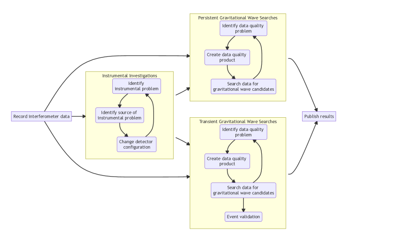
Detector characterization research in LIGO focuses on both investigations of the instruments in order to improve the future performance of the detectors and investigations of data quality in order to improve the performance of gravitational wave analyses. These data quality investigations focus on seperate types of data quality issues depedning on the gravitational-wave analysis of interest. The majority of data quality issues that impact searches for short duration, transient gravitational-wave signals do not impact searches for long duration, persistent gravitational-wave signals, and vice versa. An overview of the the connections between the multiple aspects of dectector characterization is shown in figure 1.

LIGO data is publicly distributed via the Gravitational-wave Open Science Center (GWOSC) [14]. Currently available data includes gravitational wave strain data during periods the individual detectors were observing in the first two observing runs and data quality information used in LIGO analyses [15, 16]. LIGO data from the third observing run is planned to be released in six month periods, 18 months after the start of each observing period [17]. In addition to these bulk data releases, data nearby all detected gravitational-wave events is released via GWOSC at the time of publication. Data from a subset of auxiliary channels is currently available for a three hour period around a single event [18].

Refer to caption — Figure 1: Flowchart outlining the the flow of information through various detector characterization analyses. The main areas of focus for detector characterization are instrumental investigations and data quality investigations. These data quality investigations are further broken down based on the type of gravitational-wave analysis of interest. Note that this flow chart only represents a high-level overview of the work both in this paper and in detector characterization research in general. Additional connections between detector characterization and the operation of the LIGO detectors and the analysis of LIGO data are also not shown in this flowchart. The items in this flowchart are further explained individually later in the text.

In this paper, we report the results of detector characterization methods applied to LIGO detector data from O2 and O3 to improve the performance of the detectors and astrophysical analyses. In section 2 we summarize the LIGO O2 and O3 data sets as reported in [3, 4]. In section 3 we describe major tools and infrastructure employed for LIGO detector characterization during these observing runs. In section 4 we outline work that improved the performance of the LIGO detectors by characterizing and mitigating sources of instrumental noise. In section 5 we summarize the methodology of LIGO data quality products employed by transient gravitational wave searches using O2 and O3 data as well as methods and procedures applied to LIGO detector data to validate transient event candidates. In section 6 we describe data quality investigations and products used by searches for gravitational waves from persistent sources. We conclude in section 7 with an overview of future work, including automation efforts designed to cope with the significantly higher sensitivity and expected event rate during future observing runs.

2 The O2 and O3 data sets

The O2 period spanned 268 calendar days, with the LIGO detectors participating for the entire period. Virgo, however, joined for the last 25 days. There were two scheduled breaks over the observing run; the 2016 end-of-year holidays and a few weeks in May 2017, which was used to make improvements to each of the LIGO detectors.

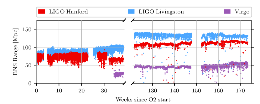
One way in which we measure sensitivity is by the binary neutron star inspiral range; this range is the distance at which a gravitational-wave signal from a the merger of two $1.4M_{\odot}$ neutron stars would be detected above a signal-to-noise ratio (SNR) of 8, averaged over all possible sky locations and inclinations without considering cosmological corrections. The LLO detector started O2 observing around 80 Mpc, and became steadily more sensitive as O2 progressed, reaching 100 Mpc. The LHO detector’s sensitivity was around 75 Mpc at the start of the observing run. It however, suffered a sudden drop in sensitivity on 6th July 2017 due to a 5.8 magnitude earthquake in Montana, finishing the run around 65 Mpc. Virgo held a steady sensitivity around 25 Mpc for its 25-day observing period. This information is illustrated in figure 2.

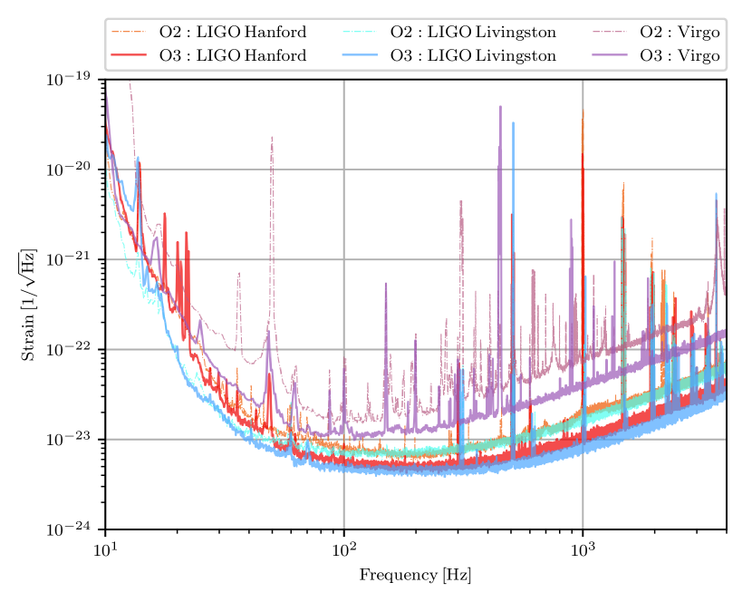
The O3 observing run was split into two periods, separated by the month of October 2019 to make stability improvements to all three detectors. The first half of the third observing run (O3a) lasted for 183 days with the LLO, LHO and Virgo detectors having a median range of 135 Mpc, 108 Mpc and 45 Mpc respectively. Due to the improvements made to the interferometers [4] between O2 and O3, the sensitivity of the detectors increased by a factor of 1.53 for LLO, 1.64 for LHO and 1.73 for Virgo. During second half of the third observing run (O3b) the sensitivity of the detectors were similar to O3a, with LLO, LHO and Virgo each having a median range of 131 Mpc, 113 Mpc and 50 Mpc. O3b lasted 147 days, some 34 days less than was originally intended. If we instead consider the sensitivity of the detectors to the inspial of two black holes each with a mass of $30M_{\odot}$ , the ranges become approximately 1425 Mpc, 1150 Mpc and 525 Mpc for LLO, LHO and Virgo respectively, throughout O3.

Figure 2 shows the typical amplitude spectral density of the strain noise for each detector over O2 and O3.

The duty cycle of each detector defines the amount of science quality data taken over a period of time. There are a number of factors which affect the duty cycle, such as the environment (e.g., weather), detector hardware (e.g., malfunctioning instrument components) and periods of commissioning. Table 1 highlights the duty cycle of each of the detectors in O2 and O3. We also give the coincident duty cycle of the LIGO detectors, as well as the triple coincident time. There is a marked improvement in the stability of the LIGO detectors between O2 and O3, with coincident science quality time increasing by some 16%. Although the Virgo duty cycle appears to decrease between observing runs, it should be highlighted that the O2 duty cycle includes livetime that is about 13 times less than in O3. As well, the 25-day O2 time that Virgo was observing for included optimal environmental conditions.

Duty Cycle
Detector	O2	O3a	O3b	O3
LHO	65%	71%	79%	75%
LLO	62%	76%	79%	77%
Virgo	85%	76%	76%	76%
LHO+LLO	46%	59%	67%	62%
LHO+LLO+Virgo	63%	44%	51%	47%

Table 1: The duty cycle (round to the nearest integer) of each of the detectors, LIGO Hanford (LHO), LIGO Livingston (LLO) and Virgo, and combinations, over the second (O2) and third observing run (O3). The O3 numbers are a combination of O3a and O3b. The Virgo and three detector duty cycles for O2 are normalized to the 25 days that Virgo joined the observing run.

In both observing runs, we used auxiliary channels that recorded the source of the instrumental noise (referred to as a “witness”) to measure sources of noise that limit detector sensitivity. Using these measurements, we were able to linearly subtract this noise from the data. During O2 a pipeline was developed to do this subtraction, which is easily adaptable to target new sources of noise as they arise [5, 19]. For both LIGO detectors this was used to target narrow line features, such as the calibration lines and 60 Hz and its harmonic frequencies. At LHO, however, there was an additional source of broadband noise known as jitter noise. This form of noise was related to the jitter of the pre-stabilized laser beam in angle and size. This was only present at LHO due to different configurations between the two LIGO detectors. By subtracting this form of noise below 1000 Hz, LHO saw an average increase in range, over O2, of 20% [19]. The LLO detector saw no appreciable increase in its range.

In O3 issues of jitter noise had been resolved, and so the same level of data cleaning was not necessary. The removal of the calibration lines and noise from their harmonics were subtracted from data as part of the calibration procedure. For a subset of gravitational wave events detected during O3, additional data cleaning was performed to remove noise contributions due to non-stationary couplings of the power mains [20].

As the interferometers are upgraded and improved, and more hardware goes into the interferometers, inevitably, there are more data quality issues that arise. For instance, O3 saw the installation of squeezed light sources [21, 22]. This is an additional system that could and did introduce additional noise into the O3 data. As the detectors become more stable, not only does their duty cycle improve, the increased observing time allows for more data quality issues to occur. These data quality issues are discussed in detail in the remainder of this paper.

3 Computing and Software

Because ground-based gravitational-wave detectors are subject to a wide range of environmental noise source and continual upgrades during an observing run, and because new technologies periodically emerge to improve sensitivity across the full frequency range, the detectors themselves are continually evolving. This presents an endless challenge to any effort to characterize noise in the detectors, as the source, shape, rate, and intensity of various noise sources is constantly changing. In this section we will outline the multiple computational solutions which have emerged to help combat this problem, focusing on the types of analyses that each software application is suited to. In doing so, we will build important context for the methods and results presented later in the paper. This section is not meant as an exhaustive list of all analysis tools that are used in detector characterization studies, but it serves to give a broad example and context for results discussed in this article.

3.1 Signal processing tools

A number of open source computing projects are developed and maintained to enable data analysis for LIGO detector characterization. These tools are published through widely used version control platforms and delivered to users through the International Gravitational-wave Network (IGWN) Conda Distribution [23]. Unless otherwise noted, they are written entirely in Python [24] and are available under terms of the GNU General Public License, version 3.0.0.

These signal processing tools are designed to both process raw timeseries that are generated by the wide variety of data streams at each observatory, as well as other pre-processed data. One of the main types of pre-processed data types that these tools are designed to ingest are “triggers” created by “event trigger generators.” A wide variety of event trigger generators exist, but in general, are designed to find excess power in data streams. These excess power bursts are considered triggers. While some event trigger generators are designed to identify generic bursts of excess power using wavelets, other event trigger generators use waveform templates from general relativity to identify triggers that are consistent with a particular gravitational-wave source.

3.1.1 GWpy

The central signal processing and data visualization engine used to prepare most figures in this paper is GWpy [25, 26], a Python package for studying data from gravitational-wave detectors. This package is designed with an extensive set of features for manipulating data in both the time and frequency domain, including:

1.

Native memory-optimized Python classes for TimeSeries and FrequencySeries objects
2.

Robust data input/output capabilities, including support for multiple file formats as well as time optimization through multithreading
3.

Custom filtering applications, digital filter designers, and convolution algorithms tailored for IGWN data
4.

An implementation of both the fast Fourier transform and the multi-Q transform (see section 3.1.3) for timeseries data
5.

A Table class primarily designed for analyzing the output of various event trigger generators
6.

Publication-quality visualization methods that are fine-tuned for every data product while remaining highly customizable

While GWpy is aimed at individual users and is relatively general-purpose, a number of other packages with narrower scope are also derived from it, as described below.

3.1.2 GW-DetChar

An extension of GWpy with specific applications to IGWN (especially LIGO) detector characterization tasks is available in the GW-DetChar software package [27]. This codebase contains a number of user modules and scripts that are able to identify and analyze known classes of glitches, such as optical scattering [28], as well as more general noise hunting algorithms such as Lasso regression [29]. For each tool in the package, the primary data product is a single webpage with responsive design features [30] which can be used to record and easily interpret results (see section 3.2.2).

3.1.3 Omega scans

A particular data visualization submodule within GW-DetChar is the gwdetchar-omega command-line tool, so named because it is a Python implementation of a legacy unmodeled transient search pipeline called Omega [31, 32, 33]. In a detector characterization context this tool is used to identify and visualize the time-frequency morphology of various sources of transient noise. Its primary data product is referred to as an omega scan, which consists of a raw multi-Q transform. The multi-Q transform consists of multiple spectrograms that tile the time-frequency plane using tiles with constant ratio of duration to bandwidth (known as the quality factor, or Q). This spectrogram tiling is referred to as the constant-Q transform [31]. The choice of Q that contains the maximum energy in a single time-frequency tile is then chosen as the optimal value of Q. This optimized raw constant-Q transform is then interpolated, providing a qualitative high-resolution image of signal energy as a function of time and frequency.

Through configuration files, users have the ability to analyze an arbitrary number of data streams over the same time range, which makes the omega scan a powerful tool in tracing the propagation of a glitch throughout interferometer subsystems. To assist with this, gwdetchar-omega can optionally cross-correlate every successive independent data stream with the signal, then display a tabulated ranking of the most highly correlated channels. Alternatively, the omega scan can be used to process gravitational wave strain streams from an arbitrary number of interferometers for a quick visual comparison of the signal morphology in each stream over a fixed time interval.

3.1.4 Omicron

The primary event trigger generator for detector characterization studies is an unmodeled transient detection pipeline called Omicron [34]. The Omicron pipeline broadly performs a multi-Q transform given some data stream, then searches for significant clusters of tiles in time-frequency space, optimizing over the quality factor. For each LIGO detector, Omicron is run on the gravitational wave strain channel and a collection of some 800-900 separate channels representing interferometer subsystems, with triggers stored in a central location from their on-site computing clusters. To ensure stability of trigger production, the workflow is managed by a Python package called pyomicron [35] and most channels have triggers available with modest 1 hour latency.

3.1.5 Hierarchical Veto

While omega scans can be used to identify correlations between an arbitrary number of data streams, such analyses tend to be confined to a narrow window of time ( $\sim 1$ sec) to understand the origin of a specific transient glitch. On the other hand, it is well worth understanding broader, longer-term correlations that may exist over the course of hours or days and to assign a statistical signifcance to the identified correlation. This is the purview of HVeto [36, 37], a companion to GW-DetChar that analyzes concurrent patterns between clusters of event triggers above a fixed SNR threshold in multiple data streams.

HVeto correlation searches are used to identify potentially statistically significant coincidences between Omicron [34] triggers in the gravitational wave strain channel and other auxiliary channels. The significance is calculated as the probability of the number of observed coincidences divided by the number expected (See [36]). HVeto is used multiple times per day to correlate glitches with auxiliary channels that may interfere with the identification of gravitational waves. When a significant association is found, HVeto analyzes the effect of removing the time segments containing the associated glitches from the analysis before proceeding to other data streams in a hierarchical fashion. With each successive round of vetoes, a list of statistically significant correlations emerges, ranked in descending order of significance. To better understand the cause of the identified correlations, omega scans of a subset of the time periods removed in each round are generated for visual inspection.

3.2 Web-based services

By contrast with the software packages described in section 3.1, the following services are maintained as broad signal processing platforms primarily accessible to the end user through the Internet, with application programming interfaces (APIs) available on the command-line and through any computing environment that supports Python. Like most LIGO and IGWN web-based services, they utilize Shibboleth Single Sign-on [38] for user authentication to ensure the security of proprietary datasets.

3.2.1 DQSEGDB

Many detector characterization tasks and pipelines designed to search for gravitational wave signals rely on data quality “flags.” Data quality flags store metadata for measured or derived states within each interferometer, its subsystems, and various components. Data quality flags are used at all current gravitational wave observatories.

These data quality flags are stored in the IGWN Data Quality Segment Database (DQSEGDB) [39]. For each flag, the database tracks spans of time (called segments) over which the flag’s on/off truth value is known. The start and end time of each segment is defined using units of integer seconds. In particular, each interferometer’s “observing mode” flag indicates segments over which that interferometer was both locked and taking science-quality data that is flagged by interferometer operators as intended for gravitational wave searches. This flag is used by all downstream analysis pipelines to distinguish spans of time that can and cannot be analyzed. Other flags can be used to reject (or veto) otherwise usable segments in which the data stream contains well-understood artifacts, such as glitches with a known cause, or planned injections of artificial test signals.

3.2.2 Detector characterization summary pages

For the convenience of LIGO commissioners, detector engineers, and data analysts, an extensive suite of detector characterization summary pages is provided [40] which offer automated daily analyses of the primary gravitational wave strain data as well as sundry interferometer subsystems. These pages are available to anyone with federated credentials on the LIGO.ORG domain, and are batch-generated on dedicated hardware with modest (0.5-1 hour) latency. The detector characterization summary pages are one of the main tools used to monitor the performance of the LIGO interferometers and the data quality. The centralized location of these automated analyses also allows for detailed follow up of any identified issues.

The raw HTML is built programmatically through the GWSumm software package [41], an extension of GWpy that also manages core signal processing, while interactive webpage elements are implemented through JavaScript. The visual layout of the front end is color-coded by interferometer, with responsive web design accomplished through Bootstrap [42] and a custom extension thereof called GW-Bootstrap [30].¹¹1To keep the file directory structure clean, these packages are published through the Node.js Package Manager (npm) [43] and supplied to the LIGO summary pages via content delivery networks.

While the LIGO detector characterization summary pages are built on-the-fly via Python code, they are also designed to be easily tunable through configuration files. Users have the freedom to register, design, and build a diverse array of visualizations, ranging from simple timeseries tracks to more complicated time-frequency spectrograms, with fine-grain control over all signal processing parameters. Because the back end utilizes Asynchronous JavaScript and XML [44] web development techniques, users also have the option to build their own custom images and HTML on the server side, then load them remotely through the summary pages. This workflow allows several third-party analyses to be hosted in one centralized location, including automated data-quality products for persistent gravitational wave searches.

While the GWSumm software package is most heavily used by LIGO, it is designed for use by the broader IGWN community. A suite of pages is currently built using the same software for the KAGRA detector [45, 46], while independent software provides a very similar service for the Virgo detector [47]. A less extensive public-facing version of the summary pages, built with GWSumm and focusing only on time segments and gravitational wave strain data, is also available [48].

3.2.3 LigoDV-web

The LIGO DataViewer Web service (LDVW) [49] is an online data visualization platform providing direct interactive access to data recorded at the LIGO Hanford and Livingston observatories and a subset of data from Virgo, KAGRA, the GEO600 observatory in Hanover, Germany [50], and the smaller 40m prototype interferometer in Pasadena, CA, USA [51]. This software instantaneously provides users with custom visualizations of small data sets in a fast, secure, and reliable manner and with minimal software, hardware, and training requirements. LDVW adds a convenient online tool that allows the generation and sharing of custom data visualizations to augment standardized analyses such as those on the Summary Pages. It is often the most convenient way to access the large number of different data sources at each site and generate large numbers of plots to address specific questions.

LDVW is implemented as a Java Enterprise application [52] with a proprietary network protocol used for data access on the back end [53]. LIGO-Virgo-KAGRA Collaboration members with proper credentials can request data to be displayed in several formats from any Internet appliance that supports a modern browser with JavaScript and minimal HTML5 support, particularly personal computers, smartphones, and tablets. The primary signal processing and image rendering engine for this service is gwpy-plot, a robust command-line interface for GWpy [25].

3.2.4 Data Quality Reports

In the context of detector characterization, a Data Quality Report (DQR) [54] is an internal collection of convenient analysis routines used to support and enable the vetting of gravitational wave event candidates. It is tightly integrated with the LIGO-Virgo Alert System (LVAlert) [55] and Gravitational-Wave Candidate Event Database (GraceDB) [56]. When an upstream search pipeline identifies a potential gravitational wave signal, the event is recorded in GraceDB and the LVAlert system broadcasts a notice to all subscribers, including the DQR architecture. When the DQR receives an alert it triggers a series of analyses from three LIGO computing clusters. Examples of included analyses are omega scans, statistical checks such as HVeto, and checks of known flags in DQSEGDB. The DQR infrastructure is modular, allowing for additional tools to be added as desired.

Within minutes of the first automated notice sent to the the Gamma-ray Coordinates Network (GCN) [57] announcing the identification of a gravitational wave event candidate, the DQR architecture begins to upload web-based reports and supporting data to GraceDB for internal review, which then informs the decision to disseminate additional GCN Notices and Circulars or to retract an announced candidate. Additional details about the tools currently implemented in the Data Quality Report and related event validation procedures are described in section 5.5.

3.2.5 Spectral artifact tools for persistent gravitational wave searches

Several different tools have been developed to aid in finding narrow, persistent spectral artifacts in gravitational wave detector data [11]. These tools build amplitude spectral density plots using fast Fourier transforms that are 1800 s, or longer, over time periods of 1-day up to an entire observing run. Since the coherent baseline is much longer than other figures-of-merit, and averaged across epochs, it allows for understanding the narrow, persistent spectral artifacts that corrupt searches for continuous gravitational waves from spinning neutron stars.

One of these tools, known as Fscan, runs automatically each day and generates 1800-s-long FFTs for the low-latency gravitational wave strain channel and a subset of auxiliary detector channels and physical environment monitoring channels. Various figures of merit can be derived from the FFT data computed from the primary gravitational wave strain channel and the subset of additional channels. This enables more regular monitoring of the behavior of spectral artifacts.

For example, normalized, day-, week-, and month-long averaged amplitude spectral densities are computed from the FFT data as well as coherence between the gravitational wave strain channel and the subset of additional channels. Correlations of spectral artifacts in ASD of different channels can then be identified via these coherence measurements as possible non-astrophysical causes of spectral artifacts. Coherence is a useful figure of merit to reject spurious coincidence of spectral artifacts that are not actually correlated and to identify potential coupling mechanisms of non-astrophysical noise into gravitational wave data.

Specifically, coherence between two channels $d_{1}(t)$ and $d_{2}(t)$ is defined as [11]

\Gamma(f)=\frac{\langle|\tilde{d}^{\star}_{1}(f)\tilde{d}_{2}(f)|^{2}\rangle}{\langle|\tilde{d}_{1}(f)|^{2}\rangle\langle|\tilde{d}_{2}(f)|^{2}\rangle},

(1)

where $\tilde{d}_{i}(f)$ ( $i=1,2$ ) is the Fourier transform of the time series data $d_{i}(t)$ , ^⋆ denotes complex conjugation, and the average $\langle\cdot\rangle$ refers to an average over $N$ segments. For Gaussian, uncorrelated noise, the expected distribution of the coherence is given by

p(\Gamma)\propto e^{-\Gamma N},

(2)

where $N$ is the number of segments used for averaging.

Other examples of figures of merit include: FineTooth, a comb identification and tracking tool; NoEMi, a line monitoring and database tool; a coherence tool database that enables efficient look-up of coherences in different time- and frequency-intervals; and studies that fold time-domain data at periodic intervals to check for periodic elevated noise. Additional figures of merit are under development for future use to aid understanding of spectral artifacts in gravitational wave detector data.

4 Instrumental Investigations

On top of a simple Michelson interferometer, Advanced LIGO detectors employ a number of technologies to increase the overall sensitivity [1]. The 4 km long Fabry-Perot cavities, also known as X and Y arms, increases the total interaction time of the main laser beam with the gravitational wave. The use of recycling cavities enhances the detector’s response to a passing gravitational wave. At the symmetric end of Michelson, the power recycling cavity amplifies the total laser power transmitted to the LIGO arms. The signal recycling cavity on the anti-symmetric end is used to vary the frequency response of the detector. Figure 1 in [6] contains a detailed schematic of the Advanced LIGO detector. Additional important subsystems for the operation and characterization of the LIGO detectors are the phyiscal environment monitoring subsystem, which includes a large array of sensors that track any changes to the environment around the detectors [58, 59], and the squeezer subsystem, which is used to inject squeezed light into the detectors and reduce residual noise from the quantum state of the laser [22, 21, 60].

In order to maximize the opportunities for the discovery of astrophysical gravitational-wave signals, it is essential to understand the instrumental and environmental noise that can mimic or obscure such signals. Recognition of potential noise couplings can lead to detector hardware changes to reduce the rate of noise artifacts. In this section, we first describe our approach to identifying instrumental noise and mitigating its effects on astrophysical searches. Later we discuss the major types and sources of transient noise and their impact on detector data quality.

4.1 Instrumental Investigation methods

4.1.1 Data Quality Monitoring

The LIGO instruments are delicate in the sense that glitches or other manifestations of noise can appear in the gravitational wave strain channel. During the observing period, a “shifter” assigned at each site conducts a week long data quality shift. The objective of the data quality shifter is to monitor the behavior of the instruments, note any changes, and to communicate them to the commissioners at LHO and LLO and the members of the detector characterization group. The LIGO summary pages [40] are the typical launching point for off-site data quality investigations of instrument noise. These pages provide both an overview of the detector status and the low-level information about specific detector subsystems. The summary pages also display the results of analysis algorithms that identify or correlate noise in both auxiliary sensors and gravitational-wave strain data. The computing infrastructure of the summary pages is discussed in further detail in section 3.2.2.

Omega scans, HVeto, Lasso [29, 27] and Omicron are some of the most commonly used analysis tools for identifying noise in the detector. Tracking down sources of transient noise often begins with the output of Omicron (see section 3.1.4), which finds short-duration bursts of noise. The resulting events, or “triggers”, can be plotted in the time-frequency plane to visualize transient noise in both witness auxiliary sensor and gravitational wave strain data. For each day, the Omicron triggers (glitches) for the gravitational wave channel are shown on a time-frequency plot with the markers color-coded for SNR. An increase in the number of high SNR glitches indicates a change in the instrument or environment. If glitches persist at specific frequencies critical to data analysis, they constitute a problem for event detection and parameter estimation. Therefore, it is essential to eliminate the harmful influence of these glitches on the searches for events. To recognize the potential sources of problematic glitches, we use HVeto (see section 3.1.5) to identify witness auxiliary sensors whose bad behavior coincides with the appearance of a subclass of glitches.

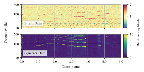
As an example of the value of data quality monitoring, we consider the “squeezer wandering line” at LHO as described here [62, 63]. A line-like feature with changing frequency was clearly visible in hourly spectrograms of the gravitational-wave strain (see figure 3). This equally spaced comb of lines will appear and disappear suddenly between 80 Hz and 140 Hz at LHO. Similar wandering lines were noticed at LLO between 160 Hz and 200 Hz. This feature was shown to be correlated in time and frequency with a strong feature in several squeezer channels at both the detectors. The data quality issue was solved by turning off the amplitude stabilizer for the laser used to provide squeezed light at LLO [61]. This was then also implemented successfully at LHO to cure the problem [64]. See [65, 66] for examples of additional solved transient noise issues.

4.1.2 Physical Environment Monitoring

Environmental noise can affect a LIGO detector by limiting its sensitivity to astrophysical gravitational wave signals and producing transients in the strain data. Some environmental noise sources can potentially be correlated between detector sites, making them particularly problematic for astrophysical searches. It is, therefore, important to identify these sources and mitigate their effects. The methodology and hardware for investigating environmental noise are discussed in detail in [58, 59]. They typically consist of generating a “noise injection” of known amplitude and frequency range and observing the detector’s response to the signal. Sensors that monitor the physical environment are used to measure the injection and estimate the noise source’s coupling to the detector. For example, we estimate acoustic coupling by using accelerometers and microphones to measure acoustic noise injections made from speakers. The sensors are much more sensitive to environmental noise than the detector is, making them good witnesses of noise sources that couple into the gravitational wave strain channel. Other injection methods include shaking injections for studying seismic coupling, magnetic field injections for coupling due to permanent magnets and electronics, and radio-frequency electromagnetic injections for radio frequencies coupling to electronics in the interferometer controls. Coupling functions are used to assess the need for mitigation as well as to estimate the contribution of transients to the gravitational wave strain channel, such as when validating gravitational wave events [67, 68].

Environmental investigations were used to track down the source of a $48$ Hz peak in the gravitational wave strain channel at LHO throughout O3a [69]. Injections using shakers and speakers showed that the noise was originating from somewhere in the corner station. Further investigation using physical impulses pointed specifically to the area near the vertex area. A new technique, whereby two shakers inject sine waves at slightly different frequencies to produce beats in the injection amplitude, showed that the beats in the motion of a particular vacuum chamber door correlated the most with the resulting beats in the gravitational wave strain channel. The noise was found to be the result of scattered light through the chamber viewports and was promptly mitigated by blocking the scattered beams, eliminating the $48$ Hz peak from the gravitational wave channel [59].

4.1.3 Safety studies

Many LIGO detector characterization analyses aim to ensure that gravitational-wave candidates are astrophysical and not caused by terrestrial noise. These analyses, such as the iDQ framework described in section 5.1, typically search for statistical correlations between auxiliary channels measuring the environment surrounding the detectors and the gravitational wave strain channel. If strong correlations are found, these gravitational wave candidates may be attributable to environmental noise and hence vetoed. This process breaks down, however, if there are auxiliary channels which pick up disturbances in the gravitational wave channel. In that case, an astrophysical signal may appear in both the gravitational wave channel and such an auxiliary channel, and the signal may subsequently be erroneously vetoed due to the channel’s correlation. Hence, information about the coupling of auxiliary channels to the gravitational wave channel is essential. Auxiliary channels which may record excess power originating in the gravitational wave channel are considered “unsafe” for vetoes, and the channels which are not found to be coupled in this way are then classified as “safe.” Only “safe” channels are used in the vetoing of gravitational wave candidates. These categorizations of channels are referred to as“safety” studies.

Since transfer functions between the strain channel and most auxiliary channels are not well known or understood, channel safety is determined empirically via hardware injection safety studies. These are conducted by injecting sine-Gaussian signals of various frequencies and amplitudes directly into the strain channel. In O3, a new set of injections was designed with wider time intervals between injections, since event trigger generators such as Omicron and KleineWelle [70], used in the subsequent safety analyses of the hardware injections, were found to be unable to distinguish between successive injections when they were spaced fewer than about three seconds apart. These injected signals range in frequency from 20 Hz to 700 Hz, with amplitudes corresponding to SNRs ranging from 15 to 500 [71, 72]. Each signal of a certain frequency and amplitude was injected three times, spaced five seconds apart.

Algorithms such as the pointy statistic [73] and HVeto then run analyses on the hardware injections to generate lists of safe and unsafe channels. pointy is a null-test that uses the assumption that events in auxiliary channels are distributed according to stationary Poisson processes. For each channel, the Poisson rate is measured using a time window much larger than that of the hardware injections. Then, using the measured rates and a set of significance thresholds, pointy produces a p-value timeseries for each auxiliary channel sampled above 16 Hz. Auxiliary channels that have anomalously small p-values ²²2This is typically chosen to be about $2\times 10^{-4}$ . at the injection times are then declared to be unsafe, and the other channels are declared safe.

HVeto [36, 37] (see section 3.1.5) correlation searches are used to compare all injections to each channel analyzed by Omicron [34] in daily operation. The operation of the safety-oriented HVeto search is the same as described in section 3.1.5 without the hierarchical removal of time periods with identified correlations. This difference allows all statistically significant correlations with the injection set to be identified, even if the auxiliary channel data streams are themselves highly correlated. Channels with high significance are then visually inspected using an omega scan and glitchgrams [25] to distinguish between witnessing the injection from chance. A low threshold for significance to trigger manual follow-up is used to minimize the risk of identifying an unsafe channel as safe.

Channel safety lists are then compiled using the results of the pointy and HVeto studies. In O3, these two tools largely agreed on safety results, with most differences arising from the larger pool of channels analyzed by pointy. When disagreements were identified which could not be reconciled based on expected false alarm rates, we erred on the side of caution, declaring channels unsafe even if only one algorithm classified it as such. At each detector, approximately 55 channels were declared unsafe, representing about 2 % of the $\mathcal{O}$ (3000) auxiliary channels sampled at or above $16~{}\mathrm{Hz}$ that were analyzed.

Beyond channels which are expected to be unsafe, such as channels in the differential arm readout measurement (DARM) control loop and many of the suspension channels, the safety algorithms also identified a number of channels which we would not have expected a priori to be unsafe. For example, a set of the channels in the alignment sensing and control subsystem at LLO measuring an radio frequency photodiode at the anti-symmetric port were found to be unsafe. These channels do not directly measure the gravitational wave strain, and were thought to be far enough away from the sensing channels to be safe, but particularly loud injections were able to excite them, resulting in an unsafe classification. Even the loudest injections possible in these studies ( $\mathcal{O}(500)$ SNR), however, are not necessarily loud enough to excite all potentially unsafe channels. These include channels such as magnetometers in the electronics bay suspension rack, which are all suspected to be unsafe at high enough SNRs. The magnetometers are not themselves coupled to gravitational wave strain, but are near electronics which drive the actuation to the test mass mirrors. A sufficiently loud signal in the interferometer would require significant actuation from these electronics to keep the test mass mirrors still, which would then be detected by the magnetometers. This phenomenon is also observed in the channels which monitor the electrostatic drive power supply, as detailed in [74]. We do not foresee these potential oversights in safety classification due to the limitations of hardware injections becoming a problem in gravitational wave veto analysis, since gravitational wave signals louder than the hardware injection limit are not expected.

4.2 Known classes of instrumental noise

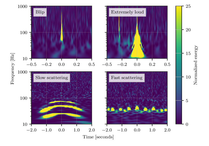
Despite the wealth of information available from the LIGO summary pages and automated algorithms to correlate noise with auxiliary channels, several classes of glitches have persisted in the data with insufficient clues to remove them all. Here, we describe some of the most frequently occurring transient noise and our efforts to identify/mitigate the noise coupling. The three most common types of glitches are Blips, Light scattering, and Loud triggers [3, 75, 76]. Spectrograms of each of these glitch classes produced using the Q-transform are shown in figure 4. These glitches are typically categorized based on their time-frequency evolution. This task is achieved for a large number of glitches through GravitySpy [76], a machine learning framework that uses the convolutional neural networks to classify transient noise based on the glitch morphology in the spectrogram. For the GravitySpy project, members of the detector characterization group helped create an initial dataset by identifying major glitch categories. Currently, this algorithm classifies transient noise into 23 different classes. The data set used to train GravitySpy, which includes information about glitches in publicly available LIGO gravitational wave strain data, is available [77]. Certain classes of transient noise, such as Blip, Tomte, Extremely Loud, and Koi-Fish, have not shown any environmental or instrumental coupling yet. Statistical data analysis of these glitch categories has led to an improved noise characterization, and we continue to look for the source of the noise. On the other hand, Scattered Light noise has shown a strong environmental coupling through the ground motion near the detectors. For one of the populations of noise due to light scattering, we were able to find the exact noise coupling through instrument investigations. Instrument changes implemented during O3b fixed the noise source, which led to an improved detector performance during high ground motion. We discuss this in more detail in section 4.2.3.

4.2.1 Blips

Blip glitches are subsecond duration glitches with high frequency bandwidth and no known instrumental or environmental coupling. Due to its appearance in time-frequency plane, as shown in the top-left of figure 4, a blip glitch may resemble a gravitational wave signal from the merger of high mass binaries. Blips occurred with a rate of approximately 2 per hour at LHO and LLO during the second observing run. This rate increased to about 4 per hour at LLO during O3, while no significant changes were observed for LHO. Blip glitches are responsible for a significant portion of the unvetoed high SNR background, reducing the effectiveness of both modeled and unmodeled searches for gravitational waves [78]. These short duration transients appear to have multiple subcategories that may be caused by different physical mechanisms, but distinguishing different types can be difficult given their short duration and simple signal morphology. In the GravitySpy citizen science project, there are other classes of glitches (called “Koi fish” and “Tomtes”) that have similarities to blips and may be related. Many investigations have been undertaken to find clues for their origin, but so far no conclusive evidence has been found to explain a mechanism for all of them [79, 80]. Weather conditions at LHO during O3 prevented the correlation between low humidity and high blip glitch rate from being observed as suggested in [81, 82]. Low energy cosmic rays striking the LIGO mirrors are responsible for a minute amount of noise in the interferometers [83, 84]. High energy cosmic rays could cause blip glitches by strongly perturbing the detector’s mirrors. By studying temporal differences between cosmic ray strikes and blip glitches at LHO, it was found that cosmic rays were not correlated with blip glitches in O2 or O3 in LHO [82].

After the conclusion of the third observing run, the light source in LHO was shut off to determine whether blip glitches occurred as a result of errors or data corruption in the interferometer’s data acquisition system [85]. No blip glitches were observed in two output mode cleaner photodiode channels, which regularly feature blip glitches during routine operations over this time period, indicating that data acquisition processes that depend on the output mode cleaner photodiodes are unlikely to be the source of blip glitches. However, some subsets of blips have been found to be correlated with instrumental issues, including computer timing errors, but this only explains some percent of them [81, 86].

4.2.2 Loud Triggers

Loud triggers in LIGO refer to short duration transients with very high SNR (SNR $>$ 100). These loud noise transients are associated with massive drops in the detector’s astrophysical range, adversely affecting its sensitivity. GravitySpy classifies most of these triggers as Extremely Loud, followed by Koi Fish. As of yet, we have not found a coupling for these loud glitches in the detector and they are consistent with a Poisson distribution. During O3, they occurred with an average rate of $3.3$ per hour at LLO and $3.5$ per hour at LHO, with a minor reduction in the rate observed in O3b compared to O3a. As the top-right of figure 4 shows, a loud glitch often saturates the time-frequency spectrogram in the band $10-500$ Hz. These triggers are witnessed by some length sensing and control channels very frequently, and the HVeto tool on the summary page consistently finds statistical correlations between some length sensing and control channels and loud triggers in gravitational wave strain. We are investigating if any issues in the length sensing and control feedback loop have any causal association with these very loud triggers in the gravitational wave strain channel. Fluctuations in voltage monitors coincident with loud triggers in the gravitational wave strain channel have been ruled out as a possible cause [74].

4.2.3 Scattered Light

Another class of noise that frequently appears in both detectors is caused when a small fraction of laser light gets scattered off of the test mass, hits a moving surface, also known as scatterer, and then rejoins the main beam. The time dependent phase difference between the main beam and the scattered beam, caused by the relative motion between the test mass and the scatterer, introduces noise in the gravitational wave channel. This noise due to light scattering shows up as arches in the time-frequency spectrograms. Its amplitude depends on the amount of scattered light that recombines with the main beam, while the maximum frequency of gravitational wave strain impacted by arches is a function of the strength of relative motion between the two surfaces. During O3, we observed two different populations of scattering transient noise: Slow Scattering and Fast Scattering.

Slow scattering triggers refer to the long duration arches visible in the time-frequency spectrograms during high ground motion in the microseism band ( $0.1-0.3$ Hz). Depending upon the amount of ground motion, these triggers would affect gravitational wave strain sensitivity in the band $20-120$ Hz. Moreover, during periods of particularly intense microseismic activity, higher frequency harmonics of the scattering arches can be seen in the spectrogram indicating multiple reflections of the scattered light beam between the test mass and the scatterer. This can be seen in the bottom-left of figure 4. During O3, we found two distinct paths in the detector through which this noise would couple to the primary gravitational wave strain channel. The identification and mitigation of these noise couplings are discussed later in this section.

Fast scattering triggers, as shown in the bottom-right of figure 4, are strongly correlated with ground motion activity in 1 to 6 Hz band. Human activity near the site, trains near the Y end of LLO, and thunderstorms near the site are known to increase the rate of fast scatter [87]. As compared to slow scattering, these triggers typically have higher peak frequency, lower SNR, and lower duration. Due to differences in gravitational wave strain sensitivity and ground motion in $1-6$ Hz band, this particular class of noise is a lot more frequent at LLO than at LHO.

The LIGO end stations located at the end of 4 km long arms contain the seismic isolation system, transmission motor stage (TMS) to monitor the transmitted light, and seismometers to measure ground motion. The seismic isolation system includes a quadruple main and reaction pendulum also known as the main and reaction chain respectively. The bottommost mirror on the main chain and the reaction chain are known as end test mass (ETM) and annular end reaction mass (AERM). To keep the interferometer on resonance, optical shadow sensors and magnetic actuators and electrostatic drives installed on the reaction chain masses are used for applying control signals on the main chain [88]. A small amount of light transmitted through the ETM is received by the photodiodes on the TMS, located behind the suspension assembly at each end station. These photodiodes are used for monitoring the transmitted field that contains the information of the field circulating in the arm cavities. Figure 2 in [89] contains a schematic of LIGO end station housing.

A collection of OSEMs are positioned throughout the LIGO interferometers, capturing the motion of several optical components likely to scatter laser light. The gwdetchar-scattering algorithm [27, 28] identifies time segments in which the motion of these OSEMs can be projected between $10-60$ Hz, then produces a webpage displaying significant gravitational wave strain Omicron triggers in this frequency band during these time segments. This tool also generates an omega scan for a random sample of such Omicron triggers. Information for each UTC day of the observing run is stored as part of the LIGO summary pages, enabling analysts to not only identify scattering triggers but also to trace the broader origin of noise due to scattered light.

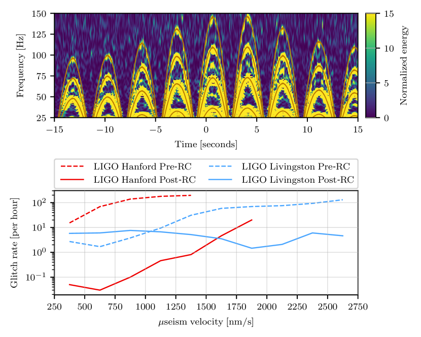
The scattering summary page hinted at a correlation between ground motion in $0.03-0.3$ Hz band and motion in the penultimate (L2) stage OSEM of the quad suspension. As shown in the top plot of figure 5, we also noticed a strong match between the fringe frequency motion of the L2 stage and the slow scattering arches in gravitational wave strain spectrogram. Other than this, HVeto suggested a statistical correlation between slow scattering in gravitational wave strain and noise in the transmitted light monitors on the TMS. A follow-up data quality investigation confirmed the existence of these two noise couplings, both via the ETM. The first coupling, which came to be known as ETM-AERM scattering is due to the scattered light between the ETM and AERM. A technique called reaction chain (RC) tracking, implemented in Jan 2020 at LLO and LHO, reduced the distance fluctuations between the ETM and AERM, which was found to be the source of noise in gravitational wave strain. Following this RC tracking at both the detectors, the slow scattering glitch rate was reduced for ground motion above 1000 $\mathrm{nm}$ /s in the microseismic band. This is shown in the bottom plot of figure 5. The second, comparatively weaker noise coupling is due to scattered light between the ETM and TMS, and is known as ETM-TMS scattering. TMS tracking, to reduce the relative motion between the ETM and TMS is in place and will be activated before the next Observing run [89].

4.2.4 Thunderstorms

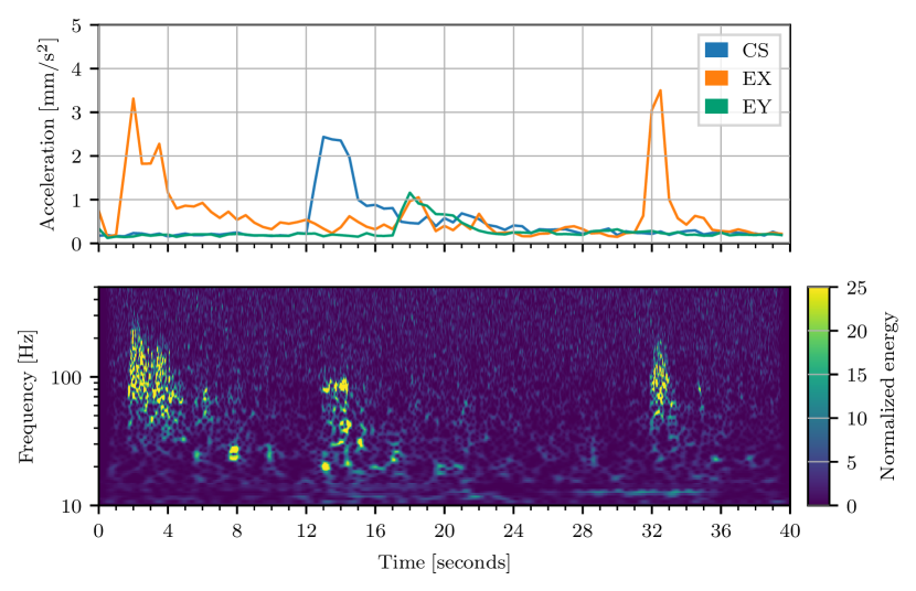
Thunderstorms are a common meteorological phenomenon in the south of Louisiana, where LLO is located. Depending on the distance from and nature of the lightning strikes, the thunderclap can range from a sharp, loud crack to a long, low rumble. The thunderclap is registered by the microphones, while the rumble is recorded by the ground motion sensors, such as accelerometers. The thunder shakes the vacuum chambers enclosing the mirrors and laser beam. One mechanism through which thunderstorms couple into the gravitational-wave detector happens when scattered light is reflected from the chamber walls and recombines to the main laser beam, producing excess noise in the gravitational-wave channel proportional to the rumbling intensity. A thunder-driven vibration was used to show that the coupling estimates from physical environment monitoring injections (see section 4.1.2) correctly predict a strong coupling between the acoustic noise at the Y-end and gravitational wave strain noise at LLO [90].

In the presence of thunder, the microphones and accelerometers attached to the vacuum chambers register disturbances at frequencies below 200 Hz, with more intensity in the band 10 Hz to 100 Hz. These acoustic and ground motion perturbations coincide with noise in the gravitational-wave channel at frequencies between 20 Hz to 200 Hz. The excess noise produces drops in the sensitivity, which is quantified by the BNS range. During the third Observing run, thunderstorms near the LLO detector provoked a range decrease of approximately 15% [91].

Thunder is unpredictable and, depending on the location of lightning, couples into the gravitational wave strain channel through one or multiple areas simultaneously. The delay in arrival time of the rumble across the different buildings allows for the localization of the source. This could be used for posterior studies about coupling mechanisms, although challenging to achieve due to possible multiple claps of thunder happening at the same time [92]. The plot at the top in figure 6, shows the root-mean-square value of the accelerometer signals after applying a band-pass filter with a frequency range 10 Hz to 100 Hz, where thunder manifest as peaks in these data. The bottom plot shows the spectrogram of the gravitational wave strain channel at the time of the same thunderstorm, where the excess noise is coincident with the thunderclaps.

4.2.5 Optical lever loud glitches

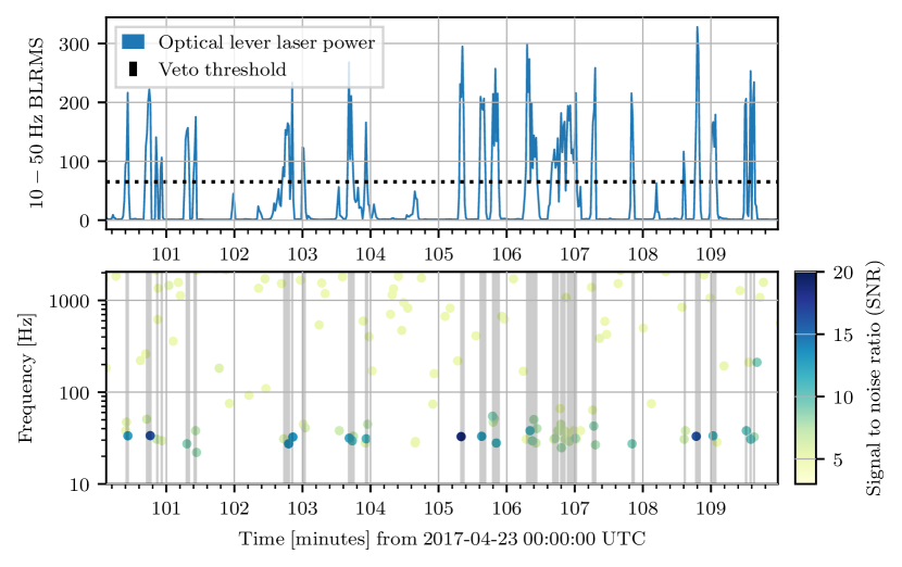
Using the summary pages to monitor the instruments helped solve several instrumental problems during O2. One example was a series of loud glitches in the gravitational-wave channel in LHO caused by glitches in the power of lasers used as optical levers. Optical levers consist of auxiliary lasers aiming light at a mirror to allow alignment at the nanoradian level [93]. If the light contributes enough photon pressure to the mirrors in an unsteady or glitchy way, this disturbance can appear in the gravitational wave channel [94]. It was first noticed in November 2016 that glitches in the end test mass at the X-end (ETMX) oplev were coupling to the gravitational wave strain [95]. While adjustments could be made to the laser power to reduce the glitching eventually, the laser was replaced in June 2017 [96]. However, glitches continued to appear in the gravitational wave strain from this cause. HVeto found statistical correlations between these glitches in gravitational wave strain and noise in the Y-end optical lever. A veto definer flag (see section 5.2) flagged gravitational wave strain glitches with SNR $>$ 65 and in the 10 Hz - 50 Hz band coincident with the noise in ETMY oplev channel. Note that these glitches appeared even though the optical lever signal was not being used in the feedback loops controlling the mirror positions. The glitches only disappeared when the ETMY oplev was turned off [97].

4.2.6 Whistles

Glitches caused by radio frequency beat notes also referred to as “whistles”, are a common source of instrumental noise coupling into the gravitational wave strain channel. They frequently appeared at LLO during O2, and in both LLO and LHO during O3. Whistles are typically identifiable by their characteristic “V” or “W” shape in frequency vs. time spectrograms. However, their frequency content and timescale vary greatly over time, meaning some very short duration whistles are difficult to resolve based on their morphology. Burst transient searches have especially been affected by whistle glitches in the last two observing runs, though matched filters can also be fooled by the part of the whistle, which increases in frequency over time in a manner similar to a compact binary merger. Outbreaks of whistle glitches were observed to correlate with oscillations in the pre-stabilized laser frequency stabilization servo loop, usually correlated with seismic activity. The issue was eventually mitigated by implementing a script to automatically adjust the pre-stabilized laser frequency stabilization system common gain [98]. Fortunately, whistles typically couple into various auxiliary channels simultaneously with the gravitational wave strain channel, so for whistle glitches in existing data it is generally relatively straightforward to construct data quality flags. Omega scans of times associated with whistles in the gravitational-wave strain channel show coincident whistles in several channels in the “length sensing and control” and “alignment sensing and control” subsystems.

4.2.7 Schumann resonances and other magnetic coupling

An important potential source of environmental correlations between gravitational wave detectors are global magnetic fields including Schumann resonances [99]. Schumann resonances are modes in the effective resonant cavity formed by the Earth’s surface and ionosphere and are excited by lightning strikes. These roughly broadband magnetic fields can couple to the gravitational wave strain channel via a variety of mechanisms, such as coupling to permanent magnets mounted on optics [100]. We have established in O3 that the magnetic noise budget is well below the sensitivity of gravitational-wave background (GWB) searches [101]. The only regular coupling to the gravitational wave strain channel from individual lighting strikes observed so far is vibrational coupling to thunderclaps (see section 4.2.4) In the future, however, it will become increasingly important to develop a detailed understanding of magnetic correlations in order to be able to make confident statements about astrophysical sources of correlation.

A correlated magnetic signal can lead to an effective, non-astrophysical GWB signal, potentially mimicking an astrophysical GWB signal. To study this possibility, we compute the coherence between magnetometers located at two sites, denoted as $M_{12}(f)$ . Additionally, we perform measurements of the coupling between magnetometer signals and the gravitational wave strain channel. These measurements allow us to compute a magnetic noise budget that can be compared with the stochastic search sensitivity, as described in [102, 100, 103, 104].

The top panel of figure 7 shows the coherence $M_{12}(f)$ in O3 computed by cross-correlating LEMI-120 magnetometers [105] between LHO and LLO. Schumann resonances are clearly visible as peaks in the coherence spectra. We also observe higher frequency correlations, which are a known environmental effect caused by lightning [106, 107].

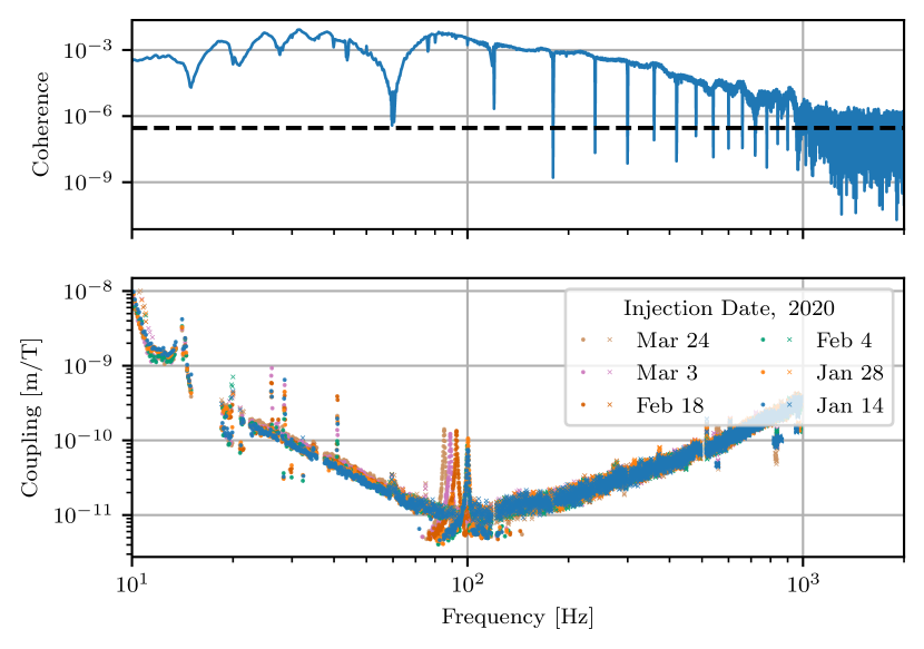
Magnetic coupling functions are measured at each detector by generating oscillating magnetic fields with a known frequency and amplitude at multiple locations around each site and measuring the resulting signal in the gravitational wave strain channel (see section 4.1.2). Results from these measurements are found at [108] and shown in the bottom panel of figure 7. In O3, we monitor time dependence of the magnetic coupling function by performing the same study weekly throughout the observing run [109, 110]. The coupling function data shown in the bottom panel of figure 7 also displays resonances at certain frequencies. These may be related to resonant motion of optics in the interferometers. Correlation between the coupling function resonances and OSEM channels is reported in [111, 112].

5 Data quality for transient gravitational wave analyses

One of the two main classes of analyses for gravitational waves is focused on identifying and interpreting gravitational waves from short duration signals. As of O3, the only source of detected gravitational waves is from compact binary coalescence (CBC) signals. These gravitational wave sources, along with other sources of short duration gravitational waves, such as supernovae [113] or cosmic strings [114], are collectively referred to as gravitational wave transients. This section outlines the main data quality products used for transient analyses in O2 and O3, data processing required to remove loud glitches, data quality methods for low latency identification of gravitational waves, and validation of candidate gravitational wave events. This includes searches for gravitational waves from CBC sources [115, 116, 117, 118, 119] and from burst sources [120, 121], as well as additional analyses completed to understand the properties of the gravitational wave source [122, 123].

5.1 Low Latency Data Quality

An important component of transient analysis is the detection and distribution of candidate gravitational wave signals as soon as possible to facilitate multi-messenger follow up [124]. In order to support these analyses, data quality products must be available with the the same or lower latency than the identification of candidates. In O2 and O3, this was accomplished with data quality products specifically designed to be used by these low latency searches and human vetting of candidates. Additional details on these procedures used in human vetting of low latency candidates and data quality information that is released alongside public alerts can be found in section 5.5.

The first data quality products are produced and distributed directly alongside the calibrated gravitational wave strain data. These include two data streams, the state vector and the data quality vector (data quality vector). The state vector is a time-series (recorded at 16 Hz) which contained information about the overall operating state of the detector, the presence of any hardware injections, and the status of the online calibration pipeline encoded as a bit-vector. The operating status information was limited to an indication that the interferometer was ready to take observation-quality data, that the site operators had transitioned to an intended observing mode, and that both the data was of observation quality and the calibration of the data was successful. This information could then immediately be used by search pipelines to know which data should be processed, while the information on hardware injections [125] could be used to excise these simulated events from analysis results searching for true gravitational waves. Finally, the additional information describing the state of the calibration could be used to track the performance of the calibration code, but was designed to be extraneous for the search pipelines themselves.

The data quality vector is a time-series (also recorded at 16 Hz) which contained information about the presence of well-known noise sources in the data, again encoded as a bit-vector. Because the data quality vector was distributed at the same time as the calibrated strain, it was able to be made available with effectively zero latency, but was limited in scope. This vector indicated the presence of several types of interferometer control-loop saturations. A prominent example of these was the glitch located very close temporarily with, and subsequently subtracted from, GW170817 in LLO [7, 126, 8]. These saturations occur when control actuation signals rail against software limits, thereby producing short-duration, broadband excess noise. Importantly, the data quality vector, like the data quality flags described in section 5.2, only encoded binary state information, and several searches used the data quality vector to automatically reject candidates [127, 128].

In addition to the state and data quality vectors, an additional data product, the iDQ [129] timeseries, was generated in low latency in O2 and O3. iDQ is a statistical inference framework which identifies non-Gaussian noise in the gravitational wave strain based on auxiliary channels and produces probabilistic data quality information. Multiple iDQ timeseries are available which have different interpretations, including $p(glitch|aux)$ and log-likelihood, but all reflect the degree of non-Gaussian noise in the data. $p(glitch|aux)$ gives the probability that there is a glitch in the gravitational wave strain channel, given auxiliary channel information, $aux$ . The log-likelihood, in contrast, gives the likelihood ratio between the glitch and clean models. $p(glitch|aux)$ is computed from the log-likelihood and also contains prior odds folding in the glitch rate within the detector.

In O3, candidates were released publicly for multi-messenger follow up without initial human vetting through GWCelery [130, 131]. These public alerts were distributed via GCN with latencies as low as a few seconds after merger. At such a low latency, few data quality products are available: the aforementioned state and data quality vectors, and the iDQ timeseries detailing statistics such as $P$ (glitch) and log(likelihood) (iDQ is discussed further in section 5.2). GWCelery included a detector characterization task which was required to be passed before the distribution of any public alert. This task checked the values of the state vector for a short window of a few seconds centered about the gravitational-wave candidate’s event time. The check would pass only if the detectors were in observing mode and no hardware injections were found. The information available from iDQ $P$ (glitch) was not a part of these automated checks, but was reported for human inspection.

Early in O3, GWCelery also checked the data quality vector to ensure there were no overflows, but this check was removed once all search pipelines switched to using gated data (see section 5.3) to avoid vetoing an overflow that would have been gated out prior to the search. All candidates passing this check were assigned the ”DQOK” label in Gravitational-Wave Candidate Event Database.

Moving forward, further automation of low latency data quality is planned for the fourth observing run (O4) and beyond (see section 7). Further integration of iDQ into the automated stack of data quality checks and within low latency search pipelines themselves, is a priority, especially as search pipelines approach and achieve negative latency where binary inspirals are detected before merger (i.e., early-warning alerts [132, 133, 134, 135]) for O4.

5.2 Data Quality Products

As a part of searches for gravitational wave transients, multiple types of data quality products are used to indicate the state of the detector and the analyzed data, with the goal of increasing the sensitivity of the searches and reducing the number of false alarms. In addition to the data quality products available in low latency, available data quality products include data quality flags, lists of time segments identifying specific data quality concerns, and higher latency predictions of the data quality from iDQ.

When a period of time demonstrating excess noise has been identified along with an auxiliary channel that witnesses the source of the noise, the associated time periods of gravitational wave strain data are marked as likely to contain instrumental artifacts using a data quality flag. A list of data quality flags that indicate periods of noisy data is then provided to astrophysical searches. For CBC searches, two tiers of data quality flags are produced: category 1 and category 2. An additional tier of data quality flags, category 3, was used by some unmodeled transient searches. When data quality flags used by the searches are referred to as daat quality vetoes.

Category 1 vetoes indicate that the data have been severely impacted by noise and should not be analyzed at any stage of an astrophysical analysis. These problems can indicate either challenges for the searches due to significant changes to the properties of noise in the detectors or gravitational wave strain data that is not correctly calibrated. Category 1 vetoes are defined using segments stored in the DQSEGDB (see section 3.2.1), and hence the start and end times must be integer seconds. However, many category 1 vetoes last multiple hours. Reasons for category 1 vetoes include incorrect detector configurations, data dropouts, and on-site maintenance work [136]. In a subset of these cases, operator logs are used to define the category 1 segments instead of auxiliary channel witnesses. Data from segments flagged by category 1 vetoes are not ingested by astrophysical analyses. Because category 1 vetoes prevent the detection of gravitational-wave candidates from the time period they flag, this veto category is not used unless a data segment is not analyzable. In O2 and O3, category 1 vetoes removed less than $2.0\%$ of analyzable data at each detector.

Category 2 vetoes indicate periods of time where the data is impacted by excess noise and should be treated with caution, but can still be used as input to an astrophysical analysis. Potential candidates that are identified during data flagged as category 2 are recommended to not be considered potential candidates by astrophysical search pipelines as candidates identified during this time have a higher likelihood to have been caused by instrumental artifacts than candidates identified outside category 2 periods. Category 2 vetoes are also defined using integer second segments in the same manner as categeory 1 vetoes. However, each category 2 segment generally only a few seconds in duration. Figure 8 shows an example of a category 2 veto that was developed during O2. This veto was used to flag periods of excess noise in an optical lever channel at LIGO Hanford that produced glitches in the gravitational wave strain data. Removing these short time periods removed a significant portion of the glitches with SNR $>8$ during this data stretch. Other examples of category 2 vetoes include earthquakes, thunder, and high wind conditions [136]. Information available as a part of the data quality vector is also used to create data quality flags that ingested by high latency searches as category 2 vetoes. Since category 2 vetoes also reduce the duration that a search pipeline is able to detect a gravitational wave event, utilization of these vetoes risks reducing the total number of detectable signals if the veto is not properly tuned or the amount of time removed is too large. For these reasons, new category 2 vetoes are not used by searches unless the flagged data quality issue has been shown to severely impact the search, minimizing the amount of time removed by category 2 vetoes as much as possible. In O2 and O3, CBC category 2 vetoes removed less than $0.4\%$ of analyzable data at each detector. The total amount of time removed by each category for all observing periods is shown in table 2.

Detector	CAT1	CBC CAT2	Burst CAT2	Burst CAT3
LIGO Hanford O2	1.93%	0.26%	0.35%	0.61%
LIGO Livingston O2	0.49%	0.16%	0.26%	0.33%
LIGO Hanford O3A	0.27%	0.37%	0.83%	0.19%
LIGO Livingston O3A	0.08%	0.10%	0.64%	0.15%
LIGO Hanford O3B	0.30%	0.02%	0.52%	0.41%
LIGO Livingston O3B	1.68%	0.28%	0.50%	0.17%

Table 2: Percent of single-detector time removed by each category of veto for each detector.

Unlike CBC searches, unmodeled burst transient searches cannot rely on a specific chirp-like morphology for the gravitational wave signal, which increases the difficulty of rejecting background noise compared to a matched-filter search. For these unmodeled searches, additions and extensions are made to the category 2 definitions used in CBC searches, resulting in an increase in time removed relative to the CBC definitions. While multiple unique category 2 flags were added for standard burst vetoes in O2 and O3, the majority of this increase in vetoed time was due to flags removing very loud glitches (typically SNR of $>$ 100) at both interferometers associated with light intensity dips.

For some unmodeled transient searches, e.g., [137, 138], category 3 data quality flags are also applied as a final stage after initial triggers are generated. These flags are mostly produced by the HVeto [36] algorithm (see section 4), which is run over strides of about five days total coincident observing of both LIGO interferometers to automatically identify auxiliary channels which can be used to create statistically significant vetoes. Using predetermined thresholds on veto efficiency and statistical significance, as well as durations and SNR thresholds selected by the HVeto algorithm for each channel, an additional set of data quality flags are constructed. Unlike category 1 and 2, category 3 vetoes may be of sub-second duration rather than being defined using integer seconds.

Targeted analyses, such as those investigating potential gravitational wave counterparts to gamma ray bursts [139] or fast radio bursts [140], also utilize data quality products. These targeted analyses use the same data quality products as non-targeted searches with similar search techniques. Targeted searches using matched filtering rely upon CBC data quality products, while unmodeled targeted searches use burst data quality products.

The segments for each category of veto used in analyses of LIGO data are available via GWOSC [14, 15, 16]. Veto segemnts for CBC and Burst searches are provided separately. Alongside the categories discussed in this work, segments corresponding to time periods where hardware injections are underway are also released.

To measure the effects of data quality vetoes on astrophysical searches, the PyCBC search pipeline [115] was run on O3 data with and without using category 2 data quality vetoes to remove data. Data from both LHO and LLO recorded between April 18, 2019 and April 26, 2019 was used in this comparison. In both cases, the PyCBC pipeline was ran with the exact same configuration as used in [4], but without including category 2 vetoes for one analysis. During this analysis period, the only category 2 vetoes that existed were at LLO, so all additional discussion will focus on the impact of these vetoes on the LLO data or the combined LLO and LHO analysis. These category 2 vetoes specifically vetoed noise that was due to acoustic from thunder and vibrations from a camera shutter that was inadvertently left operating on a timer while the detector was in observing mode.

Category 2 vetoes are designed to remove a higher fraction of triggers than the fraction of time that is removed. Using these two PyCBC analyses of the same time period, we can directly test if this is true. All triggers recorded by PyCBC are ranked based on the recovered matched filter SNR and multiple signal consistency tests. This ranking is referred to as the “ranking statistic.” After binning triggers based on the recovered ranking statistic, we compare the total number of triggers before and after the inclusion of category 2 data quality vetoes. This comparison, both in terms of the total number of triggers and the fractional differences in the number of triggers, is shown in figure 9. Only $0.78\%$ of data was removed by category 2 vetoes during this analysis period, but over $50\%$ of triggers were removed for some ranking statistic bins. Considering all triggers with a ranking statistic above 6.5, $42\%$ of triggers were removed. The large difference in the fraction of time removed by the data quality flags and the fraction of triggers removed shows that the data quality flags are removing time periods that produce a large number of triggers in the PyCBC search, as designed. The specific ranking statistic bins that have the highest fraction of triggers removed by the category 2 vetoes during this analysis are consistent with the amplitude of the noise that was vetoed. The data quality issues present during this analysis were particularly problematic for the analysis because they were loud enough to create significant background triggers but quiet enough to not be easily rejected by signal consistency checks.

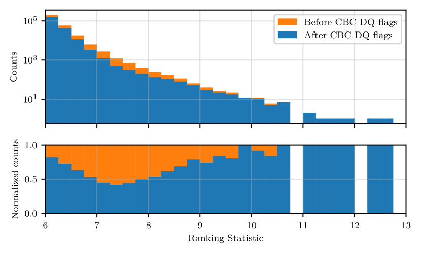
In addition to considering the total number of triggers identified by PyCBC, we also compare the sensitivity of the PyCBC search to astrophysical signals before and after the inclusion of category 2 data quality flags. The sensitivity of PyCBC is assessed by analyzing a large number of simulated signals with the analysis pipeline, and measuring the efficiency with respect to distance at which these signals are identified by the pipeline. The distance at which the pipeline recovers $50\%$ of simulated signals is referred to as the “sensitive distance.” The volume of a sphere with this distance as a radius, multipled by the total amount of time analyzed is called the volume-time. The measured volume-time of an analysis is the metric that most directly estimates the total number of real gravitational-wave signals that a pipeline could detect. We measure the volume-time of PyCBC before and after the inclusion of category 2 data quality flags. The ratio of these measured volume-time at two different significance levels, is shown in Figure 10. Since different regions of the parameter space are more susceptible to instrumental artifacts, the sensitivity measurement is broken up into several chirp mass bins.

Overall, there does appear to be a modest increase in the measured volume-time of PyCBC after including data quality flags. For the lower chirp mass bins, sensitivity does not change at a statistically significant level if noisy data are removed. This is expected, given that low mass systems produce longer duration waveforms and signal consistency tests are robust in this region of the parameter space [75]. The higher mass regions typically produce shorter duration waveforms, $\mathcal{O}$ (0.1 - 1 seconds), and can have a significant fraction of their template waveform overlap with a noise transient. Removal of noisy data results in a 5% increase in volume-time in the highest chirp mass bins. This increase is lower than observed in the first observing run (O1) [75], likely due to improvements to the PyCBC pipeline [141, 78]. The impact on the volume-time of other CBC searches is expected to be comparable to the impact on PyCBC.

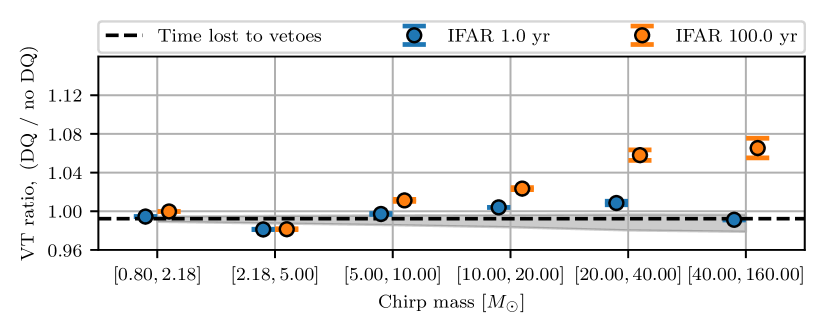
In addition to data quality flags, the iDQ [129] timeseries was used as a part of the GstLAL search pipeline in O3 [116, 142]. The generation of the higher latency iDQ dataset was identical to that of low latency iDQ, but the iDQ model was retrained using the full dataset available. Investigations into the impact of inclusion of iDQ information into the GstLAL search pipeline have also shown increases in search sensitivity [142].

5.3 Gating for transient searches

In addition to data quality products that are used in post-processing and significance calculations of transient searches, other data quality issues must be addressed by a pre-processing step. In O2 and O3, a process called “gating”, in which the data were multiplied by a smooth inverse window function, was used to remove high amplitude noise transients from gravitational wave strain data. If a noise transient has sufficient amplitude, it will ring up the whitening filters and imprint the impulse response of those filters onto the data, corrupting several seconds of data on either side of the transient [115]. Therefore simply discarding candidates that are from times impacted by these artifacts, as is done using category 2 and 3 veotes, is not sufficient to mitigate their impact. Since these transients are often sub-second in duration and the region of corrupted data is often $\mathcal{O}$ (10) seconds in duration, it is advantageous to be able to remove the sub-second glitch before the whitening filter is applied, recovering the surrounding data. The gating process multiplies the data by an inverse Tukey window which rolls smoothly from 1 to 0, zeroing out the data containing the large transient and leaving all data outside of the window unchanged [7]. This procedure was used to mitigate the impact of the glitch near GW170817 before searching the data [7, 8]

As an example of how this procedure allows for astrophysical signals to be detected by search pipelines despite the presence of a nearby loud glitch, we performed a series of injections near such a loud glitch, before and after gating, and measured the recovered ranking statistic for each injection. Simulated signals from the merger of two non-spinning $1.4M_{\odot}$ components were injected near the loud glitch at GPS time 1253878751 in gravitational wave strain data from LLO. Data from the surrounding 1024 seconds was used to calculate the power spectral estimate of the data. Each injection was then recovered using the PyCBC single-detector ranking statistic [115], before and after mitigating the glitch with the previously described gating method. The result of this study is shown in figure 11. The recovered ranking is consistent with that expected with Gaussian noise after gating the loud glitch. Without gating, the simulated signal is recovered at a much lower ranking statistic than expected, even for time periods where the signal does not overlap the glitch. When the simulated signal overlaps the glitch, the recovered ranking statistic is reduced due to signal-consistency tests that are used by PyCBC to reject instrumental artifacts. The presence of the loud glitch also biases the estimate of the power spectral density, which reduces the recovered ranking statistic during the entire period considered.

In O2 and O3, a subset of instrumental issues that were correlated with high amplitude transient noise were indicated to CBC searches using gating windows rather than data quality vetoes. While most of these glitches were sub-second in duration, they sometimes manifested at a high enough rate that consecutive gating windows were constructed, leading to several seconds of data being set to zero. To avoid underestimating the steady state noise in the detector, any gating window longer than 3 seconds in duration was considered a category 2 veto. In addition, several search pipelines implemented a complementary automatic gating procedure that constructed gating windows to remove transient noise above a set threshold on the whitened data amplitude [115, 116].

Additional methods to remove glitches exist that can more precisely remove glitches at the cost of additional computational complexity [143, 10, 144]. While gating has been shown to bias post-detection estimation of gravitational wave source properties [8], when used sparingly, gating with the windowing method discussed in this section does not measurably reduce the sensitivity of CBC searches, beyond what is expected from the amount of data removed by this process.

Similar gating methods are utilized for continuous searches, which calculate the noise spectrum over longer periods than in transient analyses, and hence are more susceptible to high-SNR glitches. The impact and methods used for these searches are discussed in section 6.

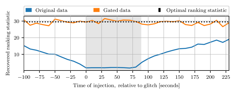
5.4 Unvetoed noise sources

Despite the wealth of information available from the LIGO summary pages and various automated algorithms to correlate noise with auxiliary channels, several classes of glitches have persisted in the data with insufficient clues to remove them all. These glitches can be categorized based on their time-frequency evolution. Three main types of glitches that have been harmful to transient searches are short duration transients, scattered light, and extremely loud glitches [3, 75].

The two main classes of short duration transients that impact the searches are blips and tomte glitches. Blip glitches (see section 4.2.1) are particularly bad for searches for high mass binary black holes and generic transients [13, 145, 146]. The short duration makes it difficult to differentiate a short astrophysical signal from a blip. Although they have not appeared in multiple detectors in coincidence more than expected due to chance, they create outliers in time-shifted backgrounds. Similar issues have been noted for tomte glitches. While blip glitches generally have power present at frequencies above the merger frequency of high mass CBC signals, tomte glitches are generally lower in frequency and better line up with a high-mass merger template. This morphology means that signal consistency tests designed to address the impact of blip glitches [78] are not as effective for tomte glitches.

Unmodeled burst searches make use of parameter space bins in order to contain problematic glitches that cannot be otherwise vetoed. One such analysis pipeline that we will consider is the coherent wave-burst (cWB) search [120]. Sorting candidates that are similar to known glitches into seperate bins and then measuring the background of each bin seperately increases the sensitivity of the other bins while still exploring the entire parameter space. The cWB search is especially sensitive to the blip class of glitches. These glitches are identified by cWB using the measured quality factor ( $Q$ ), which is the measured ratio of the energy contained in the identified candidate to the background energy from nearby data. Bin 1, which contains the majority of blip glitches, includes triggers that have a quality factor $<3$ and bin 2 contains the remaining triggers [147, 137]. Before O3 this was sufficient to contain the blip glitches. During O3, exceptionally loud and short ( ms) triggers were found polluting bin 1 enough to create a new bin to contain them. A new bin of triggers with negligible energy outside their short pulse core are separated into bin 1a while the remaining bin 1 triggers are placed in bin 1b [148]. Bin 2 contains the rest of the triggers and had the cleanest background distribution.

Another type of noise that frequently impacts searches for gravitational wave transients is scattered light. Scattered light (see section 4.2.3) especially hurts CBC searches for high spin signals, where the glitch morphology is similar to these types of systems, and long duration signals, where the chance of overlap with a scattering glitch is high. Even when the source of scattering is known, the large amount of time that is impacted by this type of glitch makes it difficult to design an effective data quality flag without removing significant amounts of data and reducing the volume-time of the searches.

Extremely loud glitches in O3 were also a severe problem for searches. While these glitches are generally removed in transient searches with gates, there are cases where glitching correlated with the extremely loud glitch, but not as loud as the main glitch, is present. These additional glitches have been shown to be a significant contribution to the background of transient searches.

There also exist data quality issues that are only partially addressed due to the limitations of current data quality products. Since data quality vetoes are designed to maximize the ratio of efficiency to deadtime, a known data quality problem may not be entirely removed if the efficiency versus deadtime is not high. This was the case for weak optical lever glitches in O2. An additional limitation of the process currently used to egenrate data quality products is that data quality flags are tuned to remove excess power from glitching, as opposed to only targeting time periods that are problematic for the search pipelines. This procedure reduces the risk of unintential bias in generating data quality flags, but also limits their effectiveness.

The combined impact of these unvetoed noise sources varies by analysis pipeline. As an example, we conducted a short study on the impact of unvetoed glitches on a CBC search for gravitational wave events coincident with externally detected gamma-ray burst (GRB) events. This study found that of high SNR injections in the LLO gravitational wave strain data that were not found by the search pipeline, approximately 35% were missed due to contamination by one of the categories of noise sources listed above. These missed injections are tests of the pipeline’s ability to detect a simulated (injected) signal within the data, and missed high SNR injections indicate that the analysis’s ability to detect gravitational waves is negatively affected by these noise sources. The noise directly reduces the effective astrophysical distance of gravitational waves to which the search is sensitive, typically defined for this type of targetted search as the distance at which $90\%$ of injections are successfully recovered [139]. The missed injections considered in this study are at distances consistent with the $90\%$ recovery distance, meaning that these noise sources are one of the limiting factors to the sensitivity of the GRB search. Thunderstorm activity, as described in section 4.2.4, had an additional impact in causing extended time segments with elevated background triggers in the searches. These impacts may be mitigated through application of additional search-specific vetoes, through additional padding of existing vetoes, and through additional identification of strong interferometer witnesses of the noise sources in the future.

5.5 Validation Procedures

An essential element of gravitational wave detection is the process of evaluating the impact of data quality issues on candidate events, known as event validation [4]. Event validation serves to both increase confidence in the astrophysical origin of gravitational-wave signals by investigating the possibility the event is instrumental in origin, as well as increasing confidence in analyses of events by evaluating the impact of any relevant data quality issues. These investigations were an important component in confirming the first detected gravitational wave event [13], and continue to be fruitful as the rate of detection increases.

In O2 and O3, event validation was completed on two timescales: within 30 minutes to multiple days of event identification [124], and weeks to months after event identification [4]. The first, low latency validation step focused on evaluating detection confidence and the impact of data quality issues on source classification and sky localization in order to support electromagnetic follow up efforts. The high-latency validation step utilized additional tools not available in low latency, such as additional statistical data quality metrics, and supported analyses of gravitational-wave source properties.

An important facet of the gravitational wave analyses in O2 and O3 was the responsibility of data quality experts to vet candidate gravitational wave signals in low latency as a part of the rapid response team, which convened to make decisions about releasing or retracting candidates for multi-messenger follow up [124]. The rapid response team was alerted whenever a significant candidate appeared, usually within a few seconds, and examined the data quality at the time of the event. Low latency searches [117, 118, 121, 120, 127, 128] require special attention due to the possibly high scientific cost of missing transient events in real-time or falsely initiating electromagnetic follow up campaigns.

The tools available to make data quality decisions matured significantly since O1. In O2, only a few data quality products were available in low latency, most notably omega scans of auxiliary data [31, 32, 27]. In O3, a large number of additional tools were generated in low latency, including additional time-frequency visualizations and monitors of the gravitational wave strain data [76, 149, 49] and data from hundreds of auxiliary channels monitoring the detectors and their environments [58, 129], as well as identification of likely sources of glitches by correlation with auxiliary channels [36, 34]. These data quality products were collated as a part of the Data Quality Report (DQR) [54], introduced in section 3.2.4.

Even including the time required for the rapid response team to review data quality products and make release decisions, significant candidates were usually announced less than 30 minutes after they were identified by the end of O2 [124]. Updates to automatically generated alerts in O3 were delivered on a similar timescale. The median reponse time of the rapid response team in O3 was 35 minutes. Based on the decision of the rapid response team, each candidate in Gravitational-Wave Candidate Event Database was assigned the ”ADVOK” label, indicating that there was not evidence to support retraction of the candidate, or the ”ADVNO” label, indicating that there was evidence to support retraction.

These low latency efforts identified numerous cases where retraction of low latency candidates was required [150, 151, 152], as well as additional cases where instrumental artifacts may potentially bias estimates of the sky localization [153, 154, 155]. One example of a retracted candidate, identified in low latency as a potential burst source, can be seen in figure 12. Visualizations of auxiliary data at the time of the event allowed identification of an auxiliary channel that is a witness to the excess power observed in the strain channel. This auxiliary channel, a monitor of a piezoelectric driver that is used to dither one of the mirrors in the output mode cleaner, suggested that the candidate was not astrophysical in origin, and was instead an instrumental artifact. Additional statistical analyses [36] of this time period were able to confirm that this correlation was statistically significant, which led to the retraction of the candidate [152].

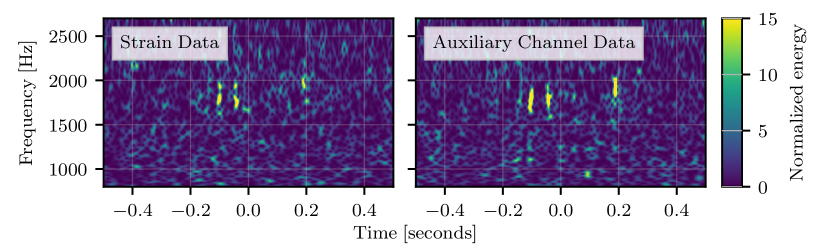
In cases where non-observing mode data is potentially used in analyses, evaluating this data is an important component of event validation [4]. While this data is generally not usable for astrophysical analyses, due to active work on the detector or lack of calibrated data, in rare instances this data has been found to be consistent with the sensitivity and data quality of typical observing periods [156, 157] after significant work to understand the data quality and calibration at the time of the events.

Event validation is especially important for short duration signals, where signal consistency tests are less powerful, and signals with extreme properties, which are more likely to be morphologically consistent with glitches. For example, the most significant intermediate mass black hole candidate in O2 was found to be consistent with an optical lever glitch, highlighted in figure 8 [158]. Conversely, event validation was an important component of confirming the astrophysical origin of the largest mass CBC source, GW190521 [159]. Candidates with high mass ratios and high spins were a large portion of the marginal candidates in GWTC-1 which were likely due to instrumental artifacts [3].

Even when a candidate is astrophysical, validation is important to evaluate potential mitigation for spurious glitches coincident with the candidate. For cases when glitches were identified, glitches were subtracted [143, 10, 19] or a reduced time duration and bandwidth was used in analyses. The increased glitch rate in O3a as compared to previous observing runs, along with an increased event rate, led to mitigation steps for 10 events in GWTC-2 [4]. A similar number of mitigations is likely required for events identified in O3b. These event validation efforts are expected to continue to play a significant role as gravitational wave detectors become more sensitive, and the source properties of gravitational wave are probed to higher precision.

6 Data quality for persistent gravitational wave searches

Searches for persistent gravitational wave sources include those for quasi-monochromatic signals from rapidly rotating neutron stars as well as stochastic backgrounds due to astrophysical or cosmological sources. Many searches have been carried out using initial LIGO/Virgo data and using Advanced LIGO/Virgo data, though no persistent signals have yet been confidently detected [160, 161, 162, 163, 164, 165, 166].

Persistent gravitational wave searches are impacted by different types of detector noise, usually by noise sources that are persistent as well. Spectral artifacts in detector data, narrow in frequency and with long-term coherence (called “lines”), pose significant challenges in analyses for persistent, narrowband gravitational wave signals [11]. Lines are typically caused by external disturbances (e.g., 60 Hz power mains, suspension resonances, electronic/magnetic coupling, etc.) that appear as artifacts in the main gravitational wave strain time series. Broadband artifacts in detector data typically do not degrade searches for persistent narrowband gravitational wave searches, but coupling of magnetic fields to the gravitational wave channel may degrade broadband gravitational wave searches [99] (see section 4.2.7). Additionally, frequent, large-amplitude transient glitches (section 4.2.2) can impact analyses for persistent gravitational waves by degrading power spectral density estimation used in these searches (see section 6.1).

Narrowband spectral artifacts in detector data can degrade searches in different ways, either obscuring or mimicking putative astrophysical signals; analogous to transient noise obscuring or mimicking transient astrophysical signals. Detection pipelines may yield many spurious outliers caused by these artifacts that require laborious follow-up or require raising significance thresholds; this leads to a lower possibility for detecting a putative persistent gravitational wave signal. Alternatively, such artifacts may obscure a real gravitational wave signal if the two are close enough so that the signal power is obscured. These two impacts lead to degraded efficiency and sensitivity of analysis pipelines.

It is therefore advantageous to mitigate—wherever possible—these spectral artifacts. Simply ignoring specific frequencies where lines may obscure a putative signal degrades the overall parameter space searched and increases the likelihood of overlooking a true signal. Where it is not possible to mitigate these artifacts, we are forced to identify the cause of the lines so that an astrophysical signal is not confused with a spectral artifact. This is a difficult, iterative process because low-level spectral artifacts require long stretches of data in order to be visible above the noise (this is essentially analogous to the long stretches of data that persistent gravitational wave signal detection analyses use). Sometimes lines may be spaced equally distant from each other in frequency and are caused by the same source; these are referred to as “combs”, where the spacing is often due to some periodic effect. Nearly all combs identified in the ASD data begin at a certain harmonic number and extend up to a cutoff harmonic, i.e., most combs do not span the entire senstive frequency band, though this is not universal. The specific details of a comb are complex and depend on factors such as the sensitivity of the detector, the source of the noise artifact, and how the noise couples into the detector data.

The first two aLIGO observing runs yielded highly sensitive data, enough for detecting multiple transient gravitational wave signals from compact binary mergers, but not yet sensitive enough for detection of persistent gravitational wave signals. An overview of the spectral artifacts from the first two observing runs may be found in [11]. Lists of spectral artifacts are also available via GWOSC [14, 15, 16]. In summary, the first observing run was found to have many lines and combs while the second observing run had fewer lines and combs, though still quite many that are problematic and many that remain unidentified [167, 168]. One of the most prolific and problematic spectral artifacts was a comb of lines, spaced 1 Hz apart, that polluted the majority of the LHO and LLO spectra in O1. This was traced to blinking light emitting diodes in the LIGO data acquisition and timing system electronics and was largely mitigated in O2 (though not entirely eliminated).

The data quality for persistent gravitational wave searches in O1 and O2 is discussed in detail in [11]; here we describe and discuss efforts to identify and mitigate spectral artifacts specifically in O3. Investigations remain ongoing to identify and mitigate sources of coupling. Given the relative improvement of LLO data in O3 compared to previous runs, we are hopeful that these mitigation efforts will continue in the future.

6.1 Self-gated gravitational wave strain for glitch impact mitigation

Large amplitude transient glitches can impact power spectral density (PSD) estimation, causing elevated noise floor levels compared to times when no glitches are present. Prior to O3, the probability for a high-amplitude transient glitch for a given stretch of coherently analyzed data was relatively low. In O3, however, the gravitational wave strain data is subject to relatively frequent and large amplitude glitches, such that the probability for one or more glitches in a given coherent segment is high. This strongly degrades analyses for persistent gravitational wave signals that rely on an accurate measurement of the noise PSD. Persistent gravitational wave searches are robust against vetoes that trigger on the loud glitches in the gravitational wave strain time series, so a scheme that removes these glitches from the data has been implemented [169]. This is referred to as “self-gating”, and is similar, though not identical to, the gating used for transient gravitational wave searches (see section 5.3).

Both approaches remove data when loud glitches occur using a smooth windowing function around each glitch time period. The novel aspect of this approach is: 1) the self-gating scheme removes data when certain band-limited-root-mean-square thresholds are exceeded; and 2) the thresholds for removal of data are much stricter so that many more large amplitude glitches are removed from the data. Further details can be found in [169].

Using self-gated data greatly improves the PSD estimation, especially for frequencies below 500 Hz. Figure 13 illustrates the improvements to the O3 run- averaged, noise-weighted ASD estimation for LHO and LLO strain data. Using the self-gating procedure mitigates the elevated noise floor by a factor of 1.5 to 3 across a broad frequency span of 20 to 250 Hz. Data that has not been cleaned of calibration lines and 60 Hz power mains lines (C01 data) [170] is degraded around those frequencies as well as the suspension violin mode resonances when using the self-gating procedure. The degraded sensitivity around calibration and power mains lines is mitigated using data that has applied all of: 1) linear subtraction of the calibration lines and power mains harmonics; 2) cleaning of the non-stationary 60 Hz sidebands [20]; and 3) self-gating of the loud glitches.

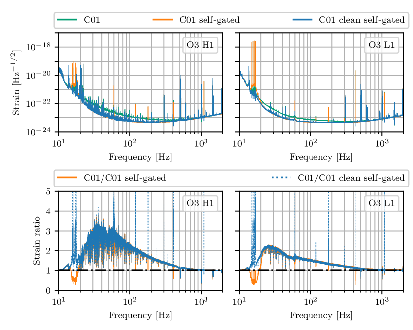
6.2 New or newly identified non-astrophysical spectral artifacts

In each observing run, narrow spectral artifacts in full-run average amplitude spectral density are flagged and, where possible, identified to be caused by certain known disturbances [11, 167, 168]. A similar approach is also employed in O3, where 7200-s-long Fourier transforms are generated—covering all of O3 observing mode epochs— averaged, and noise-weighted together in order to uncover narrow spectral features that could impact persistent gravitational wave searches. We have successfully identified several new features and summarize them below.

1.

In LHO, loud lines near 20 Hz are visible in the run-average spectra. These features are caused by sinusoidal injections into an optical alignment control loop in order to maintain stability of the angular control system. These lines could not be moved outside the LIGO LHO detection band, as they were able to do in LLO. Thus, they appear as strong spectral features with non-linear sidebands caused by mixing of the signals with low frequency (micro-)seismic noise.
2.

In both LHO and LLO, loud sinusoidal excitations are purposefully added to the control loop sensitive to the interferometer arm length differences. These generate fiducial length changes to the arm lengths and serve as calibration references (referred to as “calibration lines”). Such loud excitations, however, are observed to generate non-linearities by the digital-to-analog converters and several other spectral artifacts are found to be multiples of the fundamental frequency of the calibration lines or mixing between calibration line frequencies, e.g., $f_{1}+f_{2}$ .
3.

In both LHO and LLO, the calibration lines are also found to mix with the occasionally loud violin resonances of the suspended optics. Typically the violin resonances are not strongly excited, but there are occasional instances, following an earthquake, for example, when the resonances are excited. In these time periods, mixing between the violin resonances and calibration lines becomes apparent. Violin resonances are extremely high-Q features by design and challenging to control and damp out. They also are roughly independent, so they can be excited differently at different times. All of these features complicate mitigation of these spectral artifacts.
4.

In addition to the calibration lines located at static frequencies described in 2, at both LHO and LLO, several additional calibration lines are added to the control loop sensitive to the difference in interferometer arm lengths sequentially above 1 kHz. The actuator to add this line is not particularly strong, so the measurements require integrating for at least 1-day of low-noise operation. Once enough data is collected at a particular frequency, the line is moved to another frequency by 500 Hz for another 1-day period. After the highest frequency is reached, approximately 5 kHz, the entire process repeats, beginning again at 1 kHz. These measurements enable direct characterization of the detector performance at frequencies above 1 kHz and reduce uncertainty on systematic errors of the detector calibration [171].

6.3 Other non-astrophysical artifacts

Several other artifacts are clearly non-astrophysical, without having a clear source of noise that causes the spectral artifacts in the data. We report those artifacts here along with our understanding to date. Investigations remain ongoing into these artifacts using tools described in [11] and new approaches such as [172].

1.

Several near 1-Hz combs have been identified in LHO data. These combs are measurably different than an exact 1-Hz comb that has been largely mitigated (though not completely eliminated). The exact 1-Hz comb is caused by blinking LEDs of different GPS- synchronized electronics components [11]. It may be possible that there are un-synchronized blinking LEDs in electronics that are causing near 1-Hz combs in the data.
2.

Several 2-, 4-, 8-, and 16-Hz combs with offsets not clearly understood are found in LHO data. These combs may be linked to the digital system, since the comb tooth spacing is exactly integer values (to measurement precision of 7200-s-long FFTs). The source and coupling of this comb is not yet clearly understood.
3.

A near 30-Hz comb is observed only in LHO data with a coupling that is not yet understood. This comb was initially identified as a near 60-Hz comb, with some speculation that there may be an unidentified electrical component with poor grounding. Recognizing that the comb spacing is instead half the original identification requires further study to identify the coupling mechanism.
4.

Several unphysical, narrow, downward excursions in the gravitational wave strain noise ASD are identified near violin resonances of the suspended test masses. These artifacts indicate unphysical values in the data and should therefore be removed from persistent gravitational wave search analyses. They may be caused by either an unmodelled parasitic coupling to length control signal around the violin resonances resulting in mis-calibrated data or an overdamping of violin resonances that result in control loop “gain peaking” at adjacent frequencies.

6.4 Investigations of coherent noise

Searches for the GWB are based on cross-correlating the gravitational wave strain data between detectors [173, 174]. In order to make a statement about the presence or absence of astrophysical sources of correlation, it is crucial to understand and control noise sources that are correlated between detectors. Since GWB searches integrate over an entire observing run, the most important correlations are typically much smaller than those that affect transient searches, requiring additional analysis.

As described in section 3.2.5 and [11, 175], the coherence is measured between gravitational wave strain channels at different sites, and between the gravitational wave strain channel at one site with auxiliary channels at the same site. Coherences between gravitational wave strain channels identify frequencies with a large amount of correlation, which can be followed up by looking at coherences with auxiliary channels. Auxiliary channels not measuring the interferometer control loop sensitive to gravitational waves should have extremely low coherence with the gravitational wave strain channel. Frequency bins containing lines that are known to have an instrumental origin are removed from the analysis. Figure 14 shows a histogram of coherence values in each frequency bin between the LHO and LLO strain channels observed in O3. After removing instrumental lines, the distribution is consistent with the expectation for uncorrelated Gaussian noise in (2).

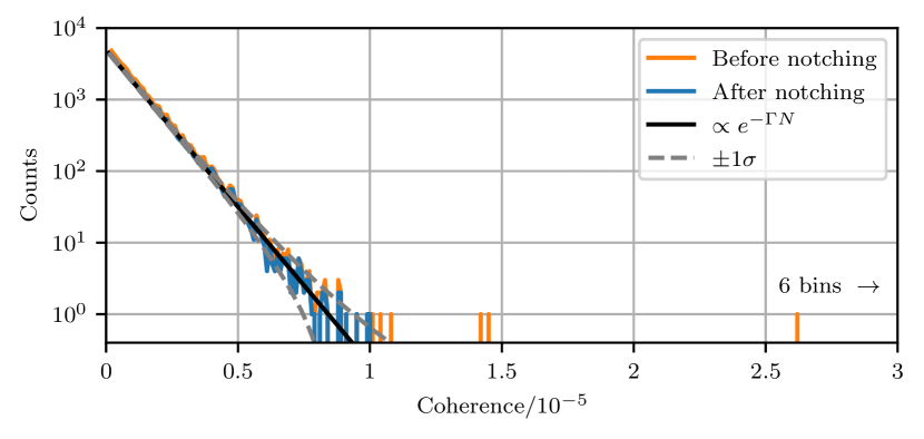
A specific example of a line follow-up with the coherence tool is illustrated by figure 15. This example shows the measured coherence between the LLO gravitational wave strain channel and a channel measuring particular angular misalignments of the interferometer readout optics. This allows rejection of spurious noise outliers that would otherwise degrade persistent gravitational wave analyses.

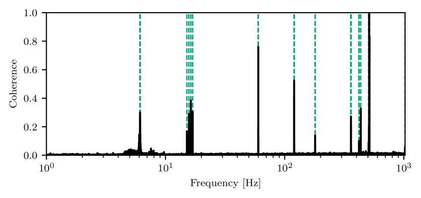
A sub-threshold comb search is used to search for the existence of combs that are coherent between the Hanford and Livingston detectors in O3. These combs may not be visible directly in the coherence measurement but may still impact searches. A large number of coherence measurements are generated from many realizations of Gaussian and uncorrelated noise. From this simulation, a background distribution is computed in order to set a threshold SNRs on combs that may be present in real data. The background distribution can then be used to assign a statistical significance for the comb-finder SNR. After removing known instrumental lines, we find that there is no statistically significant evidence of sub-threshold combs impacting the GWB search in O3. We have provided the list of frequencies removed from GWB analyses for the O1 search in [11], for O2 in [176], and for O3 in [177].

7 Future prospects

A high rate of expected detections will drive preparations for future observing runs. The rate of confident gravitational wave detections is expected to increase for the next observing run (O4) by a factor of 4 and could be as high as one detection per day [178]. At design sensitivity, the confident detection rate could be more than one per day, plus an even larger number of potentially astrophysically interesting marginal events. As the event rate grows, detector characterizations methods will require emphasis on standardization and automation to handle the large number of observed gravitational wave signals. Concurrently, there are ongoing efforts to prepare for the detection of gravitational waves from new source classes.

Upgrades to the LIGO detectors in preparation for the next observing run will introduce new components that will require additional characterization before the start of O4 [178]. The increasing duration of each observing run and expectation of high uptime will further place demands on timely identification of instrumental artifacts. To address the increase in complexity of the instruments and potential new sources of noise, statistical and machine-learning based approaches, which can more easily take advantage of the large number of data streams at each site, are expected to be used more frequently [36, 29, 179].

While the data quality methods described in prior sections were successful in enabling the confident detection of at least transient gravitational wave signals during the first three advanced-era observing runs (O1, O2, and O3a), the techniques employed were often time-consuming, even with the use of a sophisticated computational infrastructure. For example, some data quality vetoes were tuned and tested for optimum performance by hand, a process that could take days, and validation of the first several detected gravitational wave events took multiple months for each event. Tools based on machine learning methods [179] have shown promise in helping reduce the time and human input required for these efforts.

Looking forward to O4, the rapid increase in detector sensitivity will require careful planning from the LIGO detector characterization team in order to address the large number of gravitational wave detections, both from compact binaries and potentially novel sources. Detections of new gravitational wave source types, such as those from persistent gravitational wave sources, will require similar levels of development and investigation as was completed for the first gravitational wave detection [13]. More generally, we expect that the LIGO data quality and detector characterization strategy in future runs will continue to move increasingly toward automation and quantitative metrics both in low latency and for the offline analyses. Toward this end, we anticipate the growth and development of novel techniques that harness the power of the computational infrastructure supporting LIGO data quality studies.

8 Acknowledgments

The authors would like to thank members of the Virgo and KAGRA detector characterization groups who have contributed to an environment of open collaboration that enabled this work.

The authors gratefully acknowledge the support of the United States National Science Foundation (NSF) for the construction and operation of the LIGO Laboratory and Advanced LIGO as well as the Science and Technology Facilities Council (STFC) of the United Kingdom, and the Max-Planck-Society (MPS) for support of the construction of Advanced LIGO. Additional support for Advanced LIGO was provided by the Australian Research Council.

LIGO was constructed by the California Institute of Technology and Massachusetts Institute of Technology with funding from the National Science Foundation, and operates under cooperative agreement PHY-1764464. Advanced LIGO was built under award PHY-0823459. The authors are grateful for computational resources provided by the LIGO Laboratory and supported by National Science Foundation Grants PHY-0757058 and PHY-0823459. This work carries LIGO Document number P2000495.

We would like to thank all of the essential workers who put their health at risk during the COVID-19 pandemic, without whom we would not have been able to complete this work.

9 References

References

[1] Aasi J et al. (LIGO Scientific) 2015 Class. Quant. Grav. 32 074001 (Preprint 1411.4547)
[2] Acernese F et al. (VIRGO) 2015 Class. Quantum Grav. 32 024001 (Preprint 1408.3978)
[3] Abbott B et al. (LIGO Scientific, Virgo) 2019 Phys. Rev. X 9 031040 (Preprint 1811.12907)
[4] Abbott R et al. (LIGO Scientific, Virgo) 2020 (Preprint 2010.14527)
[5] Driggers J et al. (LIGO Scientific) 2019 Phys. Rev. D 99 042001 (Preprint 1806.00532)
[6] Buikema A et al. (aLIGO) 2020 Phys. Rev. D 102 062003 (Preprint 2008.01301)
[7] Abbott B P et al. 2017 Phys. Rev. Lett. 119(16) 161101
[8] Pankow C et al. 2018 Phys. Rev. D98 084016 (Preprint 1808.03619)
[9] Powell J 2018 Class. Quant. Grav. 35 155017 (Preprint 1803.11346)
[10] Cornish N J, Littenberg T B, Bécsy B, Chatziioannou K, Clark J A, Ghonge S and Millhouse M 2020 (Preprint 2011.09494)
[11] Covas P B et al. 2018 Phys. Rev. D 97 082002 (Preprint 1801.07204)
[12] Nuttall L K et al. 2015 Class. Quantum Grav. 32 245005 (Preprint 1508.07316)
[13] Abbott B P et al. (Virgo, LIGO Scientific) 2016 Class. Quant. Grav. 33 134001 (Preprint 1602.03844)
[14] Abbott R et al. 2021 SoftwareX 13 100658 ISSN 2352-7110 URL http://www.sciencedirect.com/science/article/pii/S2352711021000030
[15] LIGO Scientific Collaboration 2018 The O1 Data Release URL https://doi.org/10.7935/K57P8W9D
[16] LIGO Scientific Collaboration and Virgo Collaboration 2019 The O2 Data Release URL https://doi.org/10.7935/CA75-FM95
[17] Anderson S and Williams R 2017 LIGO Data Management Plan: June 2017 Tech. Rep. M1000066 LIGO Laboratory and LIGO Scientific Collaboration URL https://dcc.ligo.org/LIGO-M1000066/public
[18] LIGO Scientific Collaboration 2020 Auxiliary Channel Three Hour Release URL https://www.gw-openscience.org/auxiliary/GW170814/
[19] Davis D, Massinger T J, Lundgren A P, Driggers J C, Urban A L and Nuttall L K 2019 Class. Quant. Grav. 36 055011 (Preprint 1809.05348)
[20] Vajente G, Huang Y, Isi M, Driggers J C, Kissel J S, Szczepańczyk M J and Vitale S 2020 Phys. Rev. D 101(4) 042003
[21] Barsotti L, Harms J and Schnabel R 2018 Reports on Progress in Physics 82 016905
[22] Schnabel R, Mavalvala N, McClelland D E and Lam P K 2010 Nature Commun. 1 121
[23] Macleod D IGWN Conda Distribution https://computing.docs.ligo.org/conda/
[24] Van Rossum G and Drake F L 2009 Python 3 Reference Manual (Scotts Valley, CA: CreateSpace) ISBN 1441412697
[25] Macleod D, Urban A L, Coughlin S, Massinger T, Pitkin M, rngeorge, paulaltin, Areeda J, Singer L, Quintero E and Leinweber K 2020 gwpy/gwpy: 2.0.1 URL https://doi.org/10.5281/zenodo.3973364
[26] Macleod D, Urban A L, Coughlin S, Massinger T, Pitkin M, Altin P, Areeda J, Quintero E and Leinweber K 2019 GWpy: Python package for studying data from gravitational-wave detectors (Preprint 1912.016)
[27] Urban A L, Macleod D, Massinger T, Bidler J, Smith J, Macedo A, Soni S, Coughlin S, Leman K, Davis D and Lundgren A 2019 gwdetchar/gwdetchar: 1.0.2 URL https://doi.org/10.5281/zenodo.3592169
[28] Accadia T et al. 2010 Class. Quant. Grav. 27 194011
[29] Walker M, Agnew A F, Bidler J, Lundgren A, Macedo A, Macleod D, Massinger T, Patane O and Smith J R 2018 Class. Quant. Grav. 35 225002 (Preprint 1807.02592)
[30] Urban A L, Macleod D and Massinger T 2019 gwdetchar/gwbootstrap: 1.2.1 URL https://doi.org/10.5281/zenodo.3590062
[31] Chatterji S, Blackburn L, Martin G and Katsavounidis E 2004 Class. Quantum Grav. 21 S1809–S1818 (Preprint 0412119)
[32] Chatterji S 2005 The search for gravitational wave bursts in data from the second LIGO science run Ph.D. thesis Massachusetts Institute of Technology
[33] Rollins J 2010 Multimessenger Astronomy with Low-Latency Searches for Transient Gravitational Waves Ph.D. thesis Columbia University in the City of New York, LIGO-P1100009
[34] Robinet F, Arnaud N, Leroy N, Lundgren A, Macleod D and McIver J 2020 SoftwareX 100620 ISSN 2352-7110 (Preprint 2007.11374)
[35] Macleod D and Urban A L 2020 gwpy/pyomicron: 1.1.0 URL https://doi.org/10.5281/zenodo.3973543
[36] Smith J R, Abbott T, Hirose E, Leroy N, Macleod D, McIver J, Saulson P and Shawhan P 2011 Class. Quant. Grav. 28 235005 (Preprint 1107.2948)
[37] Macleod D, Urban A L, Smith J and Massinger T 2019 gwdetchar/hveto: 1.0.1 URL https://doi.org/10.5281/zenodo.3532131
[38] Shibboleth https://www.shibboleth.net
[39] Fisher R P, Hemming G, Bizouard M A, Brown D A, Couvares P F, Robinet F and Verkindt D 2020 (Preprint 2008.11316)
[40] Urban A L, Macleod D, Anderson S and Baryoga J LIGO DetChar summary pages https://summary.ligo.org
[41] Macleod D, Urban A L, Isi M, Massinger T, paulaltin, Pitkin M and Nitz A 2020 gwpy/gwsumm: 1.0.3 URL https://doi.org/10.5281/zenodo.3765457
[42] Bootstrap https://getbootstrap.com
[43] Node.js package manager https://www.npmjs.com
[44] Docs M W Ajax - Web developer guides https://developer.mozilla.org/en-US/docs/Web/Guide/AJAX
[45] Akutsu T et al. (KAGRA) 2019 Nature Astron. 3 35–40 (Preprint 1811.08079)
[46] Oshino S, Kozakai C, Yamamoto T, Kokeyama K, Soni S, Urban A L and Macleod D KAGRA DetChar summary pages https://gwdet.icrr.u-tokyo.ac.jp/~controls/summary/
[47] Hemming G Virgo Interferometer Monitor (VIM) https://vim.virgo-gw.eu
[48] Massinger T, Davis D and Urban A L IGWN Observatory Status https://www.gw-openscience.org/detector_status/
[49] Areeda J S, Smith J R, Lundgren A P, Maros E, Macleod D M and Zweizig J 2017 Astronomy and Computing 18 27–34 (Preprint 1611.01089)
[50] Grote H (LIGO Scientific Collaboration) 2010 Class. Quantum Grav. 27 084003
[51] Weinstein A 2002 Class. Quant. Grav. 19 1575–1584
[52] Oracle Corporation Java Enterprise Edition https://www.oracle.com/java/technologies/java-ee-glance.html
[53] Zweizig J, Maros E, Singer L and Areeda J Network Data Service https://computing.docs.ligo.org/daswgweb/projects/nds-client.html
[54] The LIGO Scientific Collaboration and The Virgo Collaboration 2018 Data quality report user documentation https://docs.ligo.org/detchar/data-quality-report/
[55] LVAlert https://lscsoft.docs.ligo.org/lvalert/index.html
[56] Pace A, Prestegard T, Moe B and Stephens B GraCEDb https://gracedb.ligo.org
[57] Barthelmy S D 2009 The GCN web site http://gcn.gsfc.nasa.gov/gcn/
[58] Effler A, Schofield R M S, Frolov V V, Gonzalez G, Kawabe K, Smith J R, Birch J and McCarthy R 2015 Class. Quantum Grav. 32 035017 (Preprint 1409.5160)
[59] Nguyen P et al. 2021 (Preprint 2101.09935)
[60] Tse M et al. 2019 Phys. Rev. Lett. 123 231107
[61] McCuller L 2019 aLIGO LLO Logbook 43837
[62] Lundgren A 2019 aLIGO LHO Logbook 48892
[63] Lundgren A 2019 aLIGO LHO Logbook 48772
[64] Driggers J 2019 aLIGO LHO Logbook 48949
[65] Berger B K (LIGO Scientific) 2018 J. Phys. Conf. Ser. 957 012004
[66] Nuttall L K 2018 Philosophical Transactions of the Royal Society of London A: Mathematical, Physical and Engineering Sciences 376 ISSN 1364-503X
[67] Schofield R M S et al. 2018 PEM vetting report for GW150914 Tech. Rep. LIGO-T1800505-v2 LIGO Project URL https://dcc.ligo.org/LIGO-T1800505/public
[68] Schofield R M S et al. 2018 PEM vetting report for GW170817 Tech. Rep. LIGO-T1900508-v2 URL https://dcc.ligo.org/LIGO-T1800508/public
[69] Schofield R 2020 aLIGO LLO Logbook 52184
[70] Blackburn L 2007 KleineWelle Technical Document Tech. Rep. T060221 LSC URL https://dcc.ligo.org/LIGO-T060221/public
[71] Essick R 2019 aLIGO LLO Logbook 48277
[72] Kawabe K 2019 aLIGO LLO Logbook 51736
[73] Essick R, Mo G and Katsavounidis E 2020 (Preprint 2011.13787)
[74] Nichols S 2020 aLIGO LLO Logbook 53658
[75] Abbott B P et al. (LIGO Scientific, Virgo) 2018 Class. Quant. Grav. 35 065010 (Preprint 1710.02185)
[76] Zevin M et al. 2017 Class. Quant. Grav. 34 064003 (Preprint 1611.04596)
[77] Coughlin S 2018 Updated Gravity Spy Data Set URL https://doi.org/10.5281/zenodo.1476551
[78] Nitz A H 2018 Class. Quant. Grav. 35 035016 (Preprint %****␣o3-detchar-paper.bbl␣Line␣325␣****1709.08974)
[79] Davis D 2018 aLIGO LHO Logbook 41263
[80] Helmling-Cornell A 2019 aLIGO LHO Logbook 50946
[81] Cabero M et al. 2019 Class. Quant. Grav. 36 155010 (Preprint 1901.05093)
[82] Helmling-Cornell A 2020 DCC document Tech. Rep. G2001007 LSC URL https://dcc.ligo.org/LIGO-G2001007/public
[83] Yamamoto K, Hayakawa H, Okada A, Uchiyama T, Miyoki S, Ohashi M, Kuroda K, Kanda N, Tatsumi D and Tsunesada Y 2008 Phys. Rev. D 78 022004 (Preprint 0805.2387)
[84] Braginsky V, Ryazhskaya O and Vyatchanin S 2006 Phys. Lett. A 350 1–4 (Preprint gr-qc/0509058)
[85] Schofield R 2020 aLIGO LHO Logbook 56502
[86] Helmling-Cornell A 2020 aLIGO LHO Logbook 57011
[87] Soni S 2020 Fast scattering in LIGO and Detchar noise sprint. Tech. Rep. G2001639 LSC URL https://dcc.ligo.org/LIGO-G2001639
[88] et al S M A 2012 Classical and Quantum Gravity 29 235004 URL https://doi.org/10.1088/0264-9381/29/23/235004
[89] Soni S et al. (LIGO) 2020 Class. Quant. Grav. 38 025016 (Preprint 2007.14876)
[90] Nguyen P 2019 aLIGO LLO Logbook 46025
[91] Valdes G 2020 Thunderstorms identification tool in LIGO Tech. Rep. T2000602 URL https://dcc.ligo.org/T2000602/public
[92] Valdes G 2020 Localizing Acoustic Noise Sources Affecting the Sensitivity of LIGO Through Multilateration Tech. Rep. T2000618 URL https://dcc.ligo.org/T2000618/public
[93] Aasi J et al. (LIGO Scientific Collaboration) 2015 Class. Quantum Grav. 32 074001 (Preprint 1411.4547)
[94] Covas P 2017 aLIGO LHO Logbook 37032
[95] McIver J 2016 aLIGO LHO Logbook 31810
[96] Oberling J 2017 aLIGO LHO Logbook 37027
[97] Goetz E 2017 aLIGO LHO Logbook 35798
[98] Mullavey A 2020 aLIGO LLO Logbook 51451
[99] Coughlin M W et al. 2018 Phys. Rev. D 97(10) 102007 URL https://link.aps.org/doi/10.1103/PhysRevD.97.102007
[100] Thrane E, Christensen N, Schofield R M S and Effler A 2014 Phys. Rev. D 90 023013 (Preprint 1406.2367)
[101] LIGO Scientific Collaboration and Virgo Collaboration and KAGRA Collabration 2020 Upper Limits on the Isotropic Gravitational-Wave Background from Advanced LIGO’s and Advanced Virgo’s Third Observing Run Tech. Rep. P2000314 LSC URL https://dcc.ligo.org/LIGO-P2000314/public
[102] Thrane E, Christensen N and Schofield R 2013 Phys. Rev. D 87 123009 (Preprint 1303.2613)
[103] Coughlin M W et al. 2016 Class. Quant. Grav. 33 224003 (Preprint 1606.01011)
[104] Coughlin M W et al. 2018 Phys. Rev. D 97 102007 (Preprint 1802.00885)
[105] http://www.lemisensors.com
[106] Füllekrug M and Fraser-Smith A C 2011 Geophysical Research Letters 38
[107] Ball M, Schofield R and Frey R 2020 Intersite Magnetic Signals from Lightning Tech. Rep. T2000634 LSC URL https://dcc.ligo.org/LIGO-T2000634/public
[108] Nguyen P et al. 2019 aLIGO LHO Logbook 49521
[109] Merfeld K et al. 2019 aLIGO LHO Logbook 48212
[110] Nguyen P 2021 aLIGO LHO Logbook 57672
[111] Michaloliakos I et al. 2019 aLIGO LHO Logbook 56295
[112] Michaloliakos I et al. 2019 aLIGO LHO Logbook 57390
[113] Abbott B et al. (LIGO Scientific, Virgo) 2020 Phys. Rev. D 101 084002 (Preprint 1908.03584)
[114] Abbott B et al. (LIGO Scientific, Virgo) 2018 Phys. Rev. D 97 102002 (Preprint 1712.01168)
[115] Usman S A et al. 2016 Class. Quant. Grav. 33 215004 (Preprint 1508.02357)
[116] Sachdev S et al. 2019 (Preprint 1901.08580)
[117] Adams T, Buskulic D, Germain V, Guidi G, Marion F, Montani M, Mours B, Piergiovanni F and Wang G 2016 Class. Quant. Grav. 33 175012 (Preprint 1512.02864)
[118] Chu Q 2017 Low-latency detection and localization of gravitational waves from compact binary coalescences Ph.D. thesis University of Western Australia
[119] Venumadhav T, Zackay B, Roulet J, Dai L and Zaldarriaga M 2019 Phys. Rev. D 100 023011 (Preprint 1902.10341)
[120] Klimenko S et al. 2016 Phys. Rev. D 93 042004 (Preprint 1511.05999)
[121] Lynch R, Vitale S, Essick R, Katsavounidis E and Robinet F 2017 Phys. Rev. D 95 104046 (Preprint 1511.05955)
[122] Veitch J, Raymond V, Farr B, Farr W, Graff P, Vitale S, Aylott B, Blackburn K, Christensen N, Coughlin M, Del Pozzo W, Feroz F, Gair J, Haster C J, Kalogera V, Littenberg T, Mandel I, O’Shaughnessy R, Pitkin M, Rodriguez C, Röver C, Sidery T, Smith R, Van Der Sluys M, Vecchio A, Vousden W and Wade L 2015 Phys. Rev. D 91(4) 042003 (Preprint 1409.7215)
[123] Ashton G et al. 2019 Astrophys. J. Suppl. 241 27 (Preprint 1811.02042)
[124] Abbott B et al. (LIGO Scientific, Virgo) 2019 Astrophys. J. 875 161 (Preprint 1901.03310)
[125] Biwer C et al. 2017 Phys. Rev. D 95(6) 062002
[126] Abbott B et al. (LIGO Scientific, Virgo) 2019 Phys. Rev. X 9 011001 (Preprint 1805.11579)
[127] Messick C et al. 2017 Phys. Rev. D 95 042001 (Preprint 1604.04324)
[128] Nitz A H, Dal Canton T, Davis D and Reyes S 2018 Phys. Rev. D 98 024050 (Preprint 1805.11174)
[129] Essick R, Godwin P, Hanna C, Blackburn L and Katsavounidis E 2020 Machine Learning: Science and Technology 2 015004 URL https://doi.org/10.1088/2632-2153/abab5f
[130] The LIGO Scientific Collaboration and The Virgo Collaboration 2020 Gwcelery documentation https://igwn.readthedocs.io/projects/gwcelery/en/latest/
[131] The LIGO Scientific Collaboration and The Virgo Collaboration 2018 Ligo/virgo public alerts user guide https://emfollow.docs.ligo.org/userguide
[132] Sachdev S et al. 2020 Astrophys. J. Lett. 905 L25 (Preprint 2008.04288)
[133] Kapadia S J, Singh M K, Shaikh M A, Chatterjee D and Ajith P 2020 Astrophys. J. Lett. 898 L39 (Preprint 2005.08830)
[134] Nitz A H, Schäfer M and Dal Canton T 2020 Astrophys. J. Lett. 902 L29 (Preprint 2009.04439)
[135] Magee R et al. 2021 (Preprint 2102.04555)
[136] LIGO Scientific Collaboration and Virgo Collaboration 2016 Data Quality Vetoes Applied to the Analysis of GW150914 Tech. Rep. T1600011 LSC URL https://dcc.ligo.org/LIGO-T1600011/public
[137] Abbott B P et al. (LIGO Scientific Collaboration and Virgo Collaboration) 2019 Phys. Rev. D 100(2) 024017
[138] Abbott B et al. (LIGO Scientific, Virgo) 2016 Phys. Rev. D 94 102001 (Preprint 1605.01785)
[139] Abbott R et al. (LIGO Scientific, Virgo) 2020 (Preprint 2010.14550)
[140] Abbott B et al. (LIGO Scientific, Virgo) 2016 Phys. Rev. D 93 122008 (Preprint 1605.01707)
[141] Nitz A H, Dent T, Dal Canton T, Fairhurst S and Brown D A 2017 Astrophys. J. 849 118 (Preprint 1705.01513)
[142] Godwin P et al. 2020 (Preprint 2010.15282)
[143] Cornish N J and Littenberg T B 2015 Class. Quant. Grav. 32 135012 (Preprint 1410.3835)
[144] Zackay B, Venumadhav T, Roulet J, Dai L and Zaldarriaga M 2019 (Preprint 1908.05644)
[145] Davis D, White L V and Saulson P R 2020 Class. Quant. Grav. 37 145001 (Preprint 2002.09429)
[146] Abbott B et al. (LIGO Scientific, Virgo) 2016 Phys. Rev. D 93 122004 [Addendum: Phys.Rev.D 94, 069903 (2016)] (Preprint 1602.03843)
[147] Abbott B P et al. (LIGO Scientific, Virgo) 2017 Phys. Rev. D 95 042003 (Preprint 1611.02972)
[148] Aasi J et al. (LIGO Collaboration, Virgo Collaboration) All-sky search for short gravitational-wave bursts in the third Advanced LIGO and Advanced Virgo run in preparation
[149] Mozzon S, Nuttall L K, Lundgren A, Dent T, Kumar S and Nitz A H 2020 Class. Quant. Grav. 37 215014 (Preprint 2002.09407)
[150] LIGO Scientific Collaboration and Virgo Collaboration 2019 GCN 24591 URL https://gcn.gsfc.nasa.gov/gcn3/24591.gcn3
[151] LIGO Scientific Collaboration and Virgo Collaboration 2019 GCN 25301 URL https://gcn.gsfc.nasa.gov/gcn3/25301.gcn3
[152] LIGO Scientific Collaboration and Virgo Collaboration 2019 GCN 26250 URL https://gcn.gsfc.nasa.gov/gcn3/26250.gcn3
[153] LIGO Scientific Collaboration and Virgo Collaboration 2019 GCN 24950 URL https://gcn.gsfc.nasa.gov/gcn3/24950.gcn3
[154] LIGO Scientific Collaboration and Virgo Collaboration 2019 GCN 25876 URL https://gcn.gsfc.nasa.gov/gcn3/25876.gcn3
[155] LIGO Scientific Collaboration and Virgo Collaboration 2019 GCN 26402 URL https://gcn.gsfc.nasa.gov/gcn3/26402.gcn3
[156] Abbott B P et al. 2017 The Astrophysical Journal Letters 851 L35
[157] Abbott R et al. (LIGO Scientific, Virgo) 2020 Astrophys. J. 896 L44 (Preprint 2006.12611)
[158] Abbott B P et al. (LIGO Scientific Collaboration, Virgo Collaboration) 2019 Phys. Rev. D 100 064064 (Preprint 1906.08000)
[159] Abbott R et al. (LIGO Scientific Collaboration, Virgo Collaboration) 2020 Phys. Rev. Lett. 125 101102 (Preprint 2009.01075)
[160] Abbott B P et al. 2019 The Astrophysical Journal 879 10 URL https://doi.org/10.3847%2F1538-4357%2Fab20cb
[161] Abbott B P et al. (LIGO Scientific Collaboration and Virgo Collaboration) 2019 Phys. Rev. D 99(12) 122002 URL https://link.aps.org/doi/10.1103/PhysRevD.99.122002
[162] Abbott B P et al. (LIGO Scientific Collaboration and Virgo Collaboration) 2019 Phys. Rev. D 100(2) 024004 URL https://link.aps.org/doi/10.1103/PhysRevD.100.024004
[163] Abbott B P et al. (LIGO Scientific Collaboration and Virgo Collaboration) 2019 Phys. Rev. D 100(12) 122002 URL https://link.aps.org/doi/10.1103/PhysRevD.100.122002
[164] Abbott R et al. 2020 The Astrophysical Journal 902 L21 URL https://doi.org/10.3847%2F2041-8213%2Fabb655
[165] Abbott B P et al. (LIGO Scientific and Virgo Collaboration) 2019 Phys. Rev. D 100(6) 061101
[166] Abbott B P et al. (The LIGO Scientific Collaboration and the Virgo Collaboration) 2019 Phys. Rev. D 100(6) 062001 URL https://link.aps.org/doi/10.1103/PhysRevD.100.062001
[167] LIGO Scientific Collaboration O1 Instrumental Lines https://www.gw-openscience.org/o1speclines/
[168] LIGO Scientific and Virgo Collaborations O2 Instrumental Lines https://www.gw-openscience.org/o2speclines/
[169] LIGO Scientific Collaboration 2020 Information on self-gating of $h(t)$ used in O3a continuous-wave searches Tech. Rep. T2000384 LSC URL https://dcc.ligo.org/LIGO-T2000384/public
[170] Viets A 2019 Optimizing Advanced LIGO’s scientific output with fast, accurate, clean calibration Ph.D. thesis University of Wisconsin–Milwaukee
[171] Sun L, Goetz E, Kissel J S, Betzwieser J, Karki S, Viets A, Wade M, Bhattacharjee D, Bossilkov V, Covas P B, Datrier L E H, Gray R, Kandhasamy S, Lecoeuche Y K, Mendell G, Mistry T, Payne E, Savage R L, Weinstein A J, Aston S, Buikema A, Cahillane C, Driggers J C, Dwyer S E, Kumar R and Urban A 2020 Classical and Quantum Gravity 37 225008 URL https://doi.org/10.1088/1361-6382/abb14e
[172] Harris T 2020 A Data Mining Approach to Signal Processing in Laser Interferometer Gravitational-Wave Observatory (LIGO) Fscan Data Tech. Rep. P2000185 LSC URL https://dcc.ligo.org/LIGO-P2000185/public
[173] Allen B and Romano J D 1999 Phys. Rev. D 59 102001 (Preprint gr-qc/9710117)
[174] Romano J D and Cornish N J 2017 Living Rev. Rel. 20 2 (Preprint 1608.06889)
[175] Coughlin M (LIGO Scientific, Virgo) 2010 J. Phys. Conf. Ser. 243 012010 (Preprint 1109.0330)
[176] LIGO Scientific Collaboration and Virgo Collaboration 2019 Data for a search for the isotropic stochastic background using data from Advanced LIGO’s second observing run Tech. Rep. T1900058 LSC URL https://dcc.ligo.org/LIGO-T1900058/public
[177] LIGO Scientific Collaboration and Virgo Collaboration and KAGRA Collabration 2021 Data for Upper Limits on the Isotropic Gravitational-Wave Background from Advanced LIGO’s and Advanced Virgo’s Third Observing Run Tech. Rep. G2001287 LSC URL https://dcc.ligo.org/LIGO-G2001287/public
[178] Abbott B P et al. (VIRGO, KAGRA, LIGO Scientific) 2018 Living Rev. Rel. 21 3 [Living Rev. Rel.19,1(2016)] (Preprint 1304.0670)
[179] Cuoco E, Powell J, Cavaglià M, Ackley K, Bejger M, Chatterjee C, Coughlin M, Coughlin S, Easter P, Essick R, Gabbard H, Gebhard T, Ghosh S, Haegel L, Iess A, Keitel D, Márka Z, Márka S, Morawski F, Nguyen T, Ormiston R, Pürrer M, Razzano M, Staats K, Vajente G and Williams D 2020 Machine Learning: Science and Technology 2 011002 URL https://doi.org/10.1088/2632-2153/abb93a