Improving the Data Quality of Advanced LIGO Based on Early Engineering Run Results

L. K. Nuttall¹, T. J. Massinger¹, J. Areeda², J. Betzwieser³, S. Dwyer⁴, A. Effler⁵, R. P. Fisher¹, P. Fritschel⁶, J. S. Kissel⁴, A. P. Lundgren⁷, D. M. Macleod⁸, D. Martynov^5,6, J. McIver^5,9, A. Mullavey³, D. Sigg⁴, J. R. Smith², G. Vajente⁵, A. R. Williamson¹⁰, C. C. Wipf⁵ ¹Syracuse University, Syracuse, NY 13244, USA ²California State University Fullerton, Fullerton, CA 92831, USA ³LIGO Livingston Observatory, Livingston, LA 70754, USA ⁴LIGO Hanford Observatory, Richland, WA 99352, USA ⁵LIGO, California Insitute of Technology, Pasadena, CA 91125, USA ⁶LIGO, Massachusetts Institute of Technology, Cambridge, MA 02139, USA ⁷Data Analysis Group, Albert-Einstein-Institut, Max-Planck-Institut für Gravitationsphysik, D-30167 Hannover, Germany ⁸Louisiana State University, Baton Rouge, LA 70803, USA ⁹University of Massachusetts-Amherst, Amherst, MA 01003, USA ¹⁰Cardiff University, Cardiff, CF24 3AA, UK laura.nuttall@ligo.org

Abstract

The Advanced Laser Interferometer Gravitational-wave Observatory (LIGO) detectors have completed their initial upgrade phase and will enter the first observing run in late 2015, with detector sensitivity expected to improve in future runs. Through the combined efforts of on-site commissioners and the Detector Characterization group of the LIGO Scientific Collaboration, interferometer performance, in terms of data quality, at both LIGO observatories has vastly improved from the start of commissioning efforts to present. Advanced LIGO has already surpassed Enhanced LIGO in sensitivity, and the rate of noise transients, which would negatively impact astrophysical searches, has improved. Here we give details of some of the work which has taken place to better the quality of the LIGO data ahead of the first observing run.

pacs:

04.80.Nn.

1 Introduction

The Laser Interferometer Gravitational-wave Observatory (LIGO), comprised of two 4-kilometer laser interferometers in Hanford, WA (LHO) and Livingston, LA (LLO), has been in an upgrade phase since 2010 to bring about the second generation of gravitational-wave detectors. Prior to this, LIGO was operated in two iterations, named Initial and Enhanced LIGO. The former data taking period spanned $2002-2007$ in five separate science runs; the fifth science run (November 2005 - September 2007) achieved design sensitivity in a continuous data-taking fashion [1]. The laser source and readout system were then upgraded [2], with Enhanced LIGO (science run six (S6): July 2009 - October 2010) reaching a root-mean-square strain sensitivity of $2\times 10^{-22}$ in its most sensitive frequency region ( $\sim$ 100 Hz), approximately 30% more sensitive than Initial LIGO [3].

The Advanced LIGO (aLIGO) project has completely upgraded the interferometers (this will be discussed in further detail in Section 2 [3]), which at design sensitivity will yield a factor of 10 increase in strain sensitivity. In terms of distance, aLIGO expects to be capable of detecting the merger of a binary neutron star system, averaged over sky location and orientation, to $\sim$ 200 Mpc [4]. When achieving this detection range, aLIGO is likely to detect the merger of tens of compact binary coalescences (CBCs) every year [5].

Construction of Advanced LIGO began in April 2008; early 2011 saw the first new hardware being installed. The Livingston detector was completed in mid-2014, with Hanford finishing later in the same year [3]. Both detectors have since achieved lock stretches in excess of two hours, with all of the detector’s core control systems engaged. Commissioners have since been optimizing the operation of the detectors and hunting sources of noise to improve sensitivity ahead of the first observing run (scheduled for Fall 2015).

Gravitational wave interferometer data are typically non-stationary; there are many long and short duration artifacts in the data. Long duration continuous wave searches and gravitational wave background searches are most affected by elevated noise at a given frequency, such as variations in spectral line amplitudes. This reduces the ability to search over the data at these given frequencies. However, transient gravitational wave searches (including CBCs and gravitational wave bursts) are most sensitive to short duration noise events or ‘glitches’. These can occur for a variety of reasons, including environmental or instrumental mechanisms, some of which are not fully understood. Utilizing knowledge of the expected gravitational waveform, signal-based methods are used by CBC search pipelines to distinguish between noise and a gravitational wave signal [6, 7, 8, 9]. The search pipelines also rely on studies of the behaviour of the detector to accurately remove or ‘veto’ data which are likely to contain noise artifacts. Such studies during LIGO’s sixth science run, and the improvements made to gravitational wave analyses, can be found in [10].

This paper describes efforts made to characterize the aLIGO detectors before the first observing run. Engineering runs are stretches of time where the detectors are operated as though in an observing run. Several runs have been performed to date, each scheduled at various stages of installation or detector configuration. The work presented focusses around the sixth engineering run (ER6: 8th - 17th December 2014), where only the Livingston detector participated. Many of the cases presented were found in the Livingston data, however similar artifacts were found in the Hanford data at a later date and were easily mitigated due to this early work.

The goal of this work is to identify sources of noise which would limit gravitational wave searches, track down their causes, and fix the issues at the sources (i.e. the detector). This will improve the quality of the data, reduce the amount of time needed to be vetoed from an analysis, and improve the searches performed. This work will also reduce the likelihood that a real signal will be rendered ‘suspicious’ by looking like a known glitch.

Section 2 discusses the Advanced LIGO detectors, including the upgrades which have been performed from initial LIGO. Section 3 details some of the tools and methods used to identify noise sources, with Section 4 describing examples which have been identified and mitigated. Section 5 discusses the output of the detectors, comparing early commissioned aLIGO data and data taken in S6 to more recent, mature aLIGO data. A short conclusion is given in Section 6.

2 The Advanced LIGO Interferometers

The Advanced LIGO instruments are a pair of modified Michelson interferometers that employ Fabry-Perot cavities in their arms to increase the interaction time with a gravitational wave signal [3]. A simplified schematic of the aLIGO interferometers can be seen in Figure 1 [11]. The layout of the advanced interferometers is similar in some respects to their Enhanced counterparts (for more details of the Enhanced detectors, see [2, 11, 12]).

Advanced LIGO interferometers rely on the performance of a series of interconnected subsystems to maintain stable operation. The layout of the interferometer starts with a Nd:YAG laser that generates a carrier beam at 1064 nm, [13] which is then passed through an electro-optic modulator. Here, radio-frequency (RF) sidebands are added, which are used for sensing and control of the test mass suspensions. The input mode cleaner (IMC), a triangular optical cavity, stabilizes the frequency and spatial mode content of the beam entering the heart of the interferometer. The effective laser power in the arms is increased using a power recycling cavity, which helps to improve sensitivity at higher frequencies where the detectors are limited by shot noise. New to Advanced LIGO is signal recycling, which allows the interferometer to be operated with a broader frequency response [14]. Using improved seismic isolation, test mass suspensions and heavier test masses [3], the low frequency limit on the useful sensitivity where LIGO performs an astrophysical search is pushed down from 40 Hz to 10 Hz. At higher frequencies, higher input laser power and better optical coatings [15, 16] are responsible for increased sensitivity.

Refer to caption — Figure 1: A simplified layout of the Advanced LIGO interferometers taken from [11]. The signal recycling mirror is the main change in optical layout from Enhanced LIGO.

Detection of gravitational waves in aLIGO interferometers is done by measuring the phase mismatch incurred when the two arms experience differential motion. The degree of freedom describing the differential length of the arms is labeled ‘DARM’. The instrument is considered ‘locked’ when all cavity lengths are held within their linear operating range. The differential arm length is controlled by a feedback loop and the error signal of the DARM feedback loop is calibrated to measure the external strain affecting the cavities. This signal is used to perform the astrophysical searches and, as such, is the main subject of data quality investigations.

There are a large number of recorded signals used to monitor and control the interferometers that are not directly used in the astrophysical searches, but are still extremely useful for detector characterization. These channels are referred to as auxiliary channels and can be used to track down the causes of systematic noise in DARM. Examples of these auxiliary channels include environmental monitors and signals used to control the auxiliary degrees of freedom in the instrument. These channels are used very often in detector characterization and are heavily featured in Section 4.

3 Detector Characterization Methods

The Detector Characterization¹¹1A data analysis group within the LIGO Scientific Collaboration (LSC) working to characterize the performance of the LIGO instruments, and quantify data quality as used by the search working groups [17]. group employs a diverse set of methods to assess data quality and conduct investigations when the need arises. The goal of these investigations, in general, is to ensure that a gravitational wave detection can be made should a candidate event occur. This being the case, the definition of data quality is highly dependent on how a feature in the output of the instrument is witnessed and processed by a gravitational wave search pipeline. The ideal outcome of a data quality investigation is to fix the problem at the source so that the data analyzed is clean of artifacts. The alternative outcome is to find a way to systematically identify the noise so that it can be excised from the analysis time in the form of a veto.

3.1 Starting a Data Quality Investigation

There are two common ways for a data quality investigation to arise: an unusual feature in the raw instrumental data is witnessed (such as in a spectrum or spectrogram) or an unusual feature in the output of a gravitational wave search pipeline is found. Unusual features are typically large, visible to the eye, features that are not coincident between detectors. Subsequent investigations aim to provide a complete description of instrumental features and how they influence the output of a gravitational wave search.

A convenient starting point for investigating troublesome instrumental features is the LIGO summary pages [18, 19]. These webpages house and archive the state and the behavior of the interferometer from the perspective of each subsystem with a focus on assessing data quality. There are approximately ten subsystems in total, which include, for example, the pre-stabilized laser (PSL), input mode cleaner (IMC), and alignment sensing and control (ASC) subsystems. It is common to begin an instrumental investigation by searching through the summary pages and checking each subsystem page for any clues that might identify the source of a feature.

Changes or irregularities in the DARM spectrum are more easily identified and resolved using a suite of information that includes the typical behavior of the instrument, the results of prior Detector Characterization studies, and any configuration changes noted by commissioners in the site logbook.

3.2 Data Quality Tools

A variety of tools are used to identify and pinpoint sources of noise. These include tools designed to represent the output of a typical gravitational wave search to highlight poor data quality times. Using the output of a search requires a careful understanding of the behavior of each gravitational wave search pipeline, so that signal processing artifacts are not confused for problems in the instrument. There are also tools which search for auxiliary channels that are coherent with DARM or determine the statistical significance of glitches found in both auxiliary channels and DARM.

Omicron [20], a transient search algorithm, gives a reliable account of a typical transient gravitational wave search. It is derived from an established transient search pipeline called the Q-pipeline or Omega [21], which is a transient search algorithm that produces triggers based on a sine-Gaussian excess power method. For each trigger a central time, central frequency, duration, bandwidth, Q-value and signal-to-noise ratio (SNR) (or normalised tile energy) is provided. Omicron is sensitive to most glitches and reports useful information about the properties of a glitch; it is run in quasi-real time over a large number of detector channels.

As well as being useful for assessing the data quality of a transient search, Omicron triggers can also be fed into other tools which search for interesting instrumental correlations. For example, Hierarchical Veto (HVeto) [22] reads in a set of Omicron triggers produced from DARM, and compares them to Omicron triggers produced from auxiliary channels. If there are glitches in auxiliary channels that are coincident in time with glitches in DARM to an extent that is statistically interesting, an auxiliary channel is marked as having high significance and warrants further investigation. However there are some auxiliary channels with known couplings to DARM. To thoroughly assess whether a channel directly leads to DARM, loud signals are injected in to the interferometer so that two lists of auxiliary channels can be compiled, one which is ‘safe’ and another ‘unsafe’. The unsafe channel list details the auxiliary channels with a known coupling to DARM and the safe channel list those without. It is only the safe channels which are used by tools like HVeto. Since these auxiliary channels have negligible sensitivity to gravitational waves, and therefore should not witness signals originating in the DARM degree of freedom, any statistical correlation points to an auxiliary degree of freedom with some unintended noise coupling with DARM. Examples of this procedure will be presented in Section 4.

Advanced LIGO interferometers rely on the performance of a series of interconnected subsystems to maintain stable operation. Each subsystem has a team responsible for its maintenance and commissioning. In an effort to better understand the output of the instrument and its impact on astrophysical search pipelines, the Detector Characterization group has mirrored this approach and assigned data quality liaisons to each subsystem. These subsystem liaisons are tasked with understanding the operation of their respective subsystems and are responsible for interfacing with commissioners, developing summary pages that allow those interested in data quality to have a general overview of the subsystem, and designing real-time monitoring of their subsystem’s data quality using the Online Detector Characterization (ODC) framework [23].

4 Data Quality Issues

During S6 there were numerous examples of sources of noise identified in the interferometers, which could not be fixed immediately or at all during the science run [10]. ‘Data Quality (DQ) flags’ were constructed to identify noisy times as they would adversely affect a gravitational wave search. Analysis groups would use these flags to make an informed decision on which data to analyse. Teams of people, both on and off site, have been working to identify and fix sources of noise which would impact a search for gravitational waves before the run begins. This will hopefully have the added bonus of minimizing the number of DQ flags which will need to be used by the analyses in the first observing run. The remainder of this section highlights some of the work done at both LHO and LLO to mitigate noise prior to the observing run, however focus is given to studies at LLO since this observatory has been in active commissioning longer than LHO.

4.1 DAC Calibration Glitches

In the commissioning period leading up to the 6th Engineering Run, a population of low frequency (10 Hz - 100 Hz) glitches appeared in the output of the instrument. While monitoring the locked instrument, it was noticed that these glitches were correlated with times when certain suspension control signals crossed a value of zero.

The aLIGO suspension system uses 18-bit digital-to-analog converters (DACs) to interact with various systems within the interferometers. These 18-bit DACS are composed of a 16-bit low-order DAC and a 2-bit high-order DAC. The 2-bit chip has four states which are individually calibrated (during an auto-calibration routine), and then are corrected in real-time. The calibration of the 16-bit chip is such that is occupies exactly one state of the 2-bit chip [24].

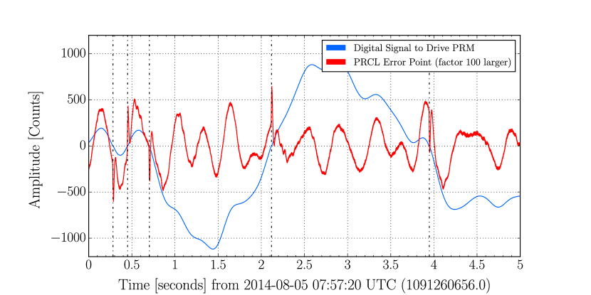
In these 18-bit DACs glitches have been observed at both sites due to an output discontinuity when the 2-bit DAC engages. This discontinuity is caused by a voltage calibration error between the 16-bit and 2-bit chips in the DAC. In these DACs, the 2-bit chip is responsible for the two highest order bits, which causes the discontinuity to occur for transitions at output values of zero and $\pm 2^{16}$ (Figure 2).

These glitches were particularly detrimental to transient search pipelines, as they increase the rate of loud, low frequency background events, making the ability to confidently identify a true signal difficult.

To fully understand the scope of the problem and its impact on astrophysical searches, software was developed that systematically searched through suspension drive signals for any instances when they crossed either zero or $\pm 2^{16}$ . Any time this happened, the time and offending suspension drive signal channel were recorded and fed in to Hveto, which was able to discover which channels had crossings that were statistically correlated with glitches in DARM. This served two purposes: it provided the capability to pinpoint which suspensions required immediate intervention to clean up the output of the instrument, and it quantitatively demonstrated the effect of the DAC calibration glitches on data quality for a transient search.

Two strategies were employed to try to mitigate this type of glitch. First, an offset was applied to the signals so they would never cross values of zero or $\pm 2^{16}$ . However, this did not fix the root problem and presented an easy opportunity for the glitches to resurface should the signals begin to drift. Offsetting the output signals to avoid these values also limit the dynamic range of the control signals being sent to the optics, which had the potential to increase the influence of noise associated with the DACs. The solution, instead, was found to be an auto-calibration routine. In this routine an internal voltage reference is used to calibrate the two chips such that when the 2-bit DAC engages a smooth transition occurs (rather than a step function). Re-calibration of the 18-bit DACs caused the discontinuity to nearly vanish [25]. It was observed, however, that over the course of a few weeks after the calibration was performed, the calibration would degrade and the discontinuity would return. Regular calibration of the 18-bit DACs in the aLIGO suspension system is required and has been implemented to minimize these glitches. More stable solutions are under study. The software mentioned previously is currently employed to continuously monitor the status of the DAC calibration and determine its correlation to glitches in DARM.

4.2 Radio Frequency Beat Notes

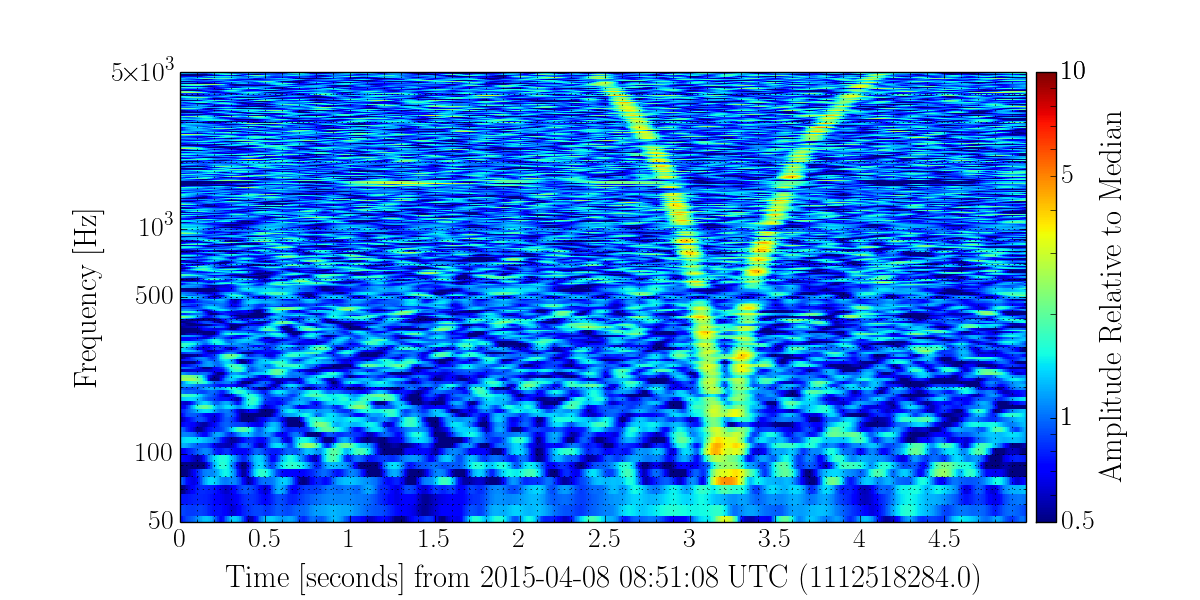
Throughout aLIGO commissioning, radio frequency beat notes in auxiliary channels have been observed and, as the noise in the instruments improved, signals caused by radio frequency beat notes became prevalent in DARM. Across a wide range of frequencies, signals were observed in DARM spectrograms with a characteristic ‘W’ or ‘V’ shape as shown in Figure 3.

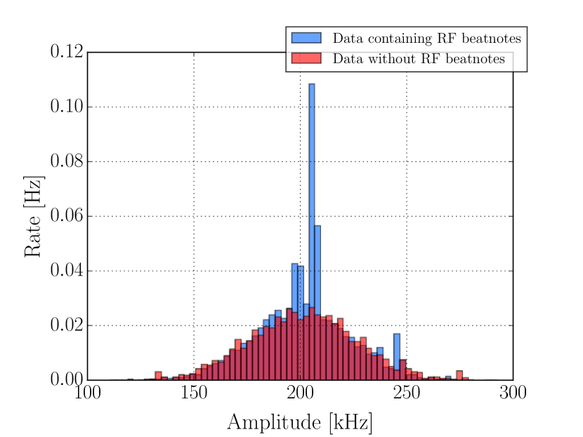
Initial investigations pointed towards a channel that monitors the detuning of the laser frequency based on the input mode cleaner length as being a good predictor of this feature. Every time this channel had particular values these beat notes would be observed in DARM, as can be seen in Figure 4. This figure shows a rate histogram of DARM triggers (as seen by Omicron) over $\sim$ six hour period binned by the corresponding channel value (blue bars). When the channel had values of $\sim$ 196-201, 204-209 and 245-250 kHz (according to Figure 4), beat notes were observed in DARM. In the absence of beat notes, the distribution of the triggers appears Gaussian (red bars).

Voltage controlled oscillators (VCOs) are used in control loops throughout the LIGO interferometers. For example, a voltage controlled oscillator in the pre-stabilized laser frequency stabilization servo (FSS) generates a radio frequency signal which drives an acousto-optic modulator (AOM). The AOM generates frequency sidebands on the laser which are used as a frequency reference in the FSS loop. This loop is used to correct frequency fluctuations in the laser by locking the frequency of the laser to the length of the input mode cleaner [26]. Beat notes between voltage controlled oscillators are visible in the stored detector output when the absolute frequency difference between two voltage controlled oscillators drops below 16 kHz.

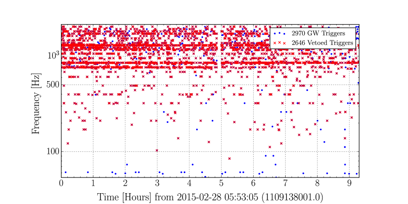
Despite efforts to keep radio frequency radiation and pick up to a minimum, beat notes can still contaminate the low noise DARM channel. It was found that these features occurred every time the frequency stabilization servo voltage controlled oscillator at LLO or LHO swept through 79.2 MHz, the same frequency as a fixed frequency fiber acousto-optic modulator. During some locks, these radio frequency beat notes were extremely problematic and were responsible for $\sim$ 90% of all glitches seen in DARM at LLO (Figure 5). When testing the binary black hole search on Livingston aLIGO data containing these radio frequency beat note glitches, they proved to greatly limit the search performance.

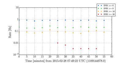
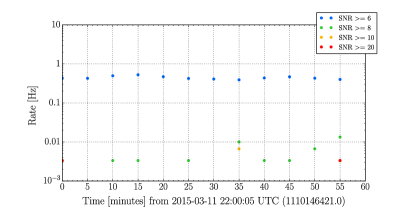
To remove these sources of glitches from DARM, the output frequencies of the problematic voltage controlled oscillators were moved away from each other in frequency. Once this had been accomplished, a dramatic decrease in the number of glitches associated to these sources was observed. At LLO, the overall glitch rate improved by a factor of two and glitches with an SNR $>$ 8 improved in rate by a factor of 50, as shown in Figure 6. However there are numerous voltage controlled oscillators with output frequencies in the same vicinity, meaning radio frequency beat notes could and have presented themselves again as commissioning continues. Due to the work presented, there are now more deterministic methods for finding and tracking these types of glitches.

4.3 Pre-Stablized Laser Periscope

The pre-stabilized laser subsystem consists of a Nd:YAG laser and control systems which stabilize the laser in beam direction, frequency, and intensity [13]. The system lives outside of the vacuum system (which houses the majority of the aLIGO hardware) in a clean, dust-free environment. The optical components of the pre-stabilized laser are located on an optical bench, which is, physically, much lower than the height the beam needs to be to enter the vacuum systems viewport. A periscope is used to elevate the beam so that it can enter the vacuum enclosure.

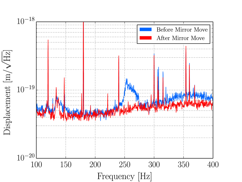
Input pointing noise can couple to DARM through several mechanisms. As shown in Figure 1, the laser beam propagates inside the input mode cleaner (IMC) before entering the main interferometer. Any jitter at the input of the IMC cavity is filtered, since the cavity is stable. However, jitter is also converted into intensity noise in transmission through a quadratic coupling, which can have a linear component if the IMC cavity is slightly misaligned. Intensity noise then couples to DARM since the Advanced LIGO detectors are using a DC readout scheme [2] in which the primary laser is sensed on a DC photodiode and used as a reference to identify gravitational wave sidebands. Clearly, one solution is to tune the IMC angular controls to improve its alignment. However, the residual misalignment was large enough to still introduce a non negligible amount of intensity noise at the input of the main interferometer. For example, two distinct features in the DARM spectrum at $\sim$ 135 Hz and $\sim$ 250 Hz were due to the resonance of a mirror mount securing a piezo-actuated mirror, used to control the beam pointing in to the input mode cleaner. This mirror mount was located at the top of the pre-stabilized laser periscope and was causing excess beam jitter. To relieve this issue, the piezo-actuated mirror was moved from the top of the pre-stabilized laser periscope to the pre-stabilized laser optical table and was replaced with a fixed mirror. This immediately improved the input pointing noise from the PSL to the vacuum enclosure, reducing the effect at 135 Hz and removing the 250 Hz resonance, as seen in Figure 7.

4.4 End Test Mass Ring Heaters

The laser power circulating in the aLIGO arms can be as large as 750 kW, which will cause deformations in the test masses via thermal expansion, changing the spatial modes of the optical field [3]. Thermal compensation techniques are used to maintain the radius of curvature of the input and end test masses, which, if left uncompensated, would increase by a few tens of meters [3]. A ring heater is one of the elements of the thermal compensation system used in aLIGO. It comprises a nickel-chromium heater wire wound around two semi-circular glass rods and radiates onto the test mass to compensate for thermo-elastic deformations of the test masses [3].

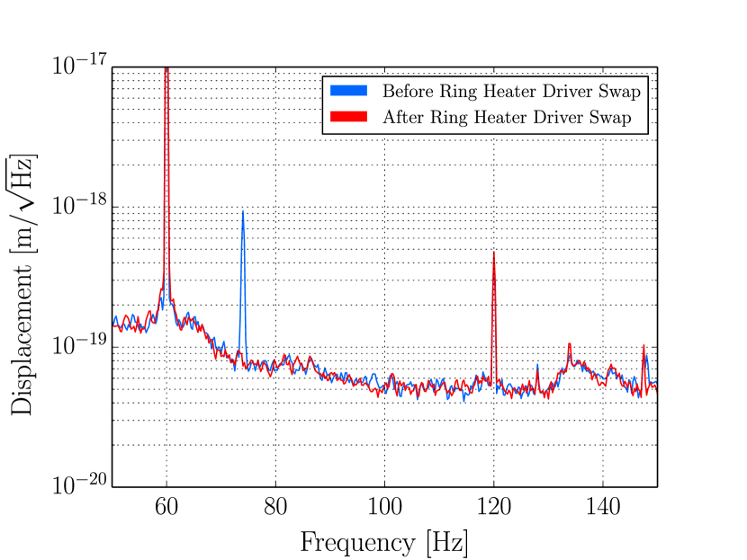
Because ring heaters actuate on the major optics of the interferometer, noise associated with them can couple significantly into DARM. This was the case for a feature found during commissioning activities at Livingston, at 74 (end X station) and 76 Hz (end Y station) in the DARM spectrum. This noise feature was found to be coherent with a magnetometer at the same end station. Upon further investigations, it was discovered the ring heater drivers were the source of the added noise. Subsequently, they were both replaced with drivers modified to have filtered power supplies. The improvement in the gravitational wave spectrum for the replacement at the Y end can be seen in Figure 8. Similar features in DARM due to the ring heaters were also seen at Hanford. This discovery and increased understanding of the potential systematic impacts of the thermal compensation system has prompted the setup of monitors which will catch such future problems.

4.5 LLO Pre-Mode Cleaner

The pre-mode cleaner (PMC) is a four mirror resonator in a bow tie configuration responsible for removing higher-order modes from the beam, reducing beam jitter, and providing low-pass filtering for radio frequency intensity fluctuations [3]. Three mirrors are fixed, while the fourth is attached to a piezoelectric transducer (PZT) to control the length of the pre-mode cleaner. In terms of the interferometer layout the pre-mode cleaner is located just before the input mode cleaner (see Figure 1)

During locking activities in early December 2014, noise between $1-2$ kHz (see Figure 10) in DARM was found to be correlated with the pre-mode cleaner system. Not only was there found to be a linear coherence between DARM and the pre-mode cleaner in this frequency range, Hveto also found the glitches in the high voltage drive that controls the PZT, which is fixed to one of the four pre-mode cleaner mirrors, to be coincident with glitches seen between $1-2$ kHz in DARM. Figure 10 shows the statistical correlation seen by HVeto.

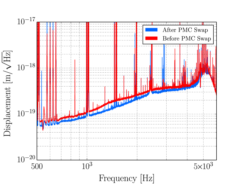
The decision was made to completely replace the pre-mode cleaner. Before the swap, however, it was discovered that cables left over from previous measurements were connected to electronics used to interact with the PMC. These additional cables were demonstrated to cause the increased noise in the DARM channel. Due to the sensitive nature of the LIGO instruments, subtle details like improperly terminated cables can have a serious impact on data quality, and people both on and off site are constantly monitoring to catch these kinds of problems. Although this additional noise in DARM was not found to be due solely to pre-mode cleaner degradation, the pre-mode cleaner was still replaced to improve other areas of operation.

5 Comparing the Initial and Advanced LIGO Performance of the LIGO Livingston Detector

The non-Gaussian, non-stationary nature of the noise in the detectors has a great impact on the ability to perform a search for gravitational waves. The glitches and features described in Section 4 would have a detrimental impact on the transient analyses had they not been removed. Loud glitches (in terms of SNR) can mask or potentially disrupt a transient gravitational wave signal in the data, whereas many quieter glitches can raise the background of a search and limit the ability to distinguish signal from noise.

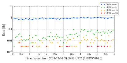
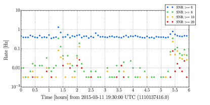
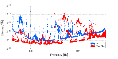
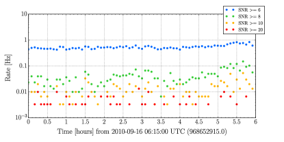
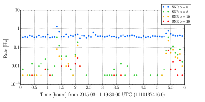
Section 5.1 looks at the aLIGO Livingston detector before and after the DQ issues discussed in Section 4 were resolved. Section 5.2 compares Livingston’s S6 detector output to the early aLIGO data after the removal of the example DQ issues. For both cases, six hours of detector data were chosen to best represents the detectors at the time of operation. The S6 data were taken from September 16th 2010, which is considered to be a typical, good, and stable stretch of data. All subsequent plots showing data from this time are labelled ‘S6’. Data from December 16th 2014, which were taken during an engineering run, contained all the DQ issues previously described and are labelled as ‘ER6’ in the subsequent plots in this section. Data from a lock stretch on March 11th 2015 were selected to represent the early aLIGO data (and is labelled ‘Post ER6’ in the following plots). In terms of data quality and inspiral range, the March 11th aLIGO data represents some of the best from that period. However, it should be noted that this latter stretch of data represents active commissioning time, where the detector is not left completely alone and is therefore not as stable as the S6 or ER6 data. Since the writing of this paper it is worth noting that another engineering run has taken place.

5.1 A Comparison of aLIGO Data, Before and After DQ Example Issues were Resolved

For two weeks in December 2014, the LIGO Livingston detector took part in an engineering run (ER6). During this time, the detector was locked as often as possible, with minimal interruption for commissioning activities, to assess the stability and quality of the data.

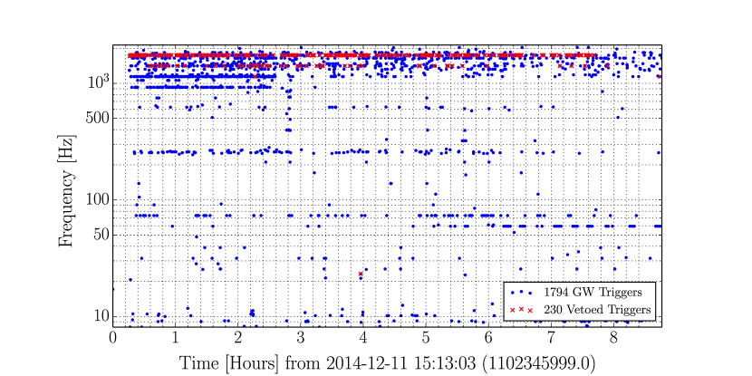
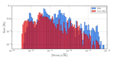
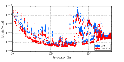
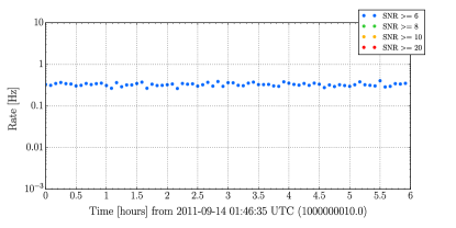
Figure 11 compares the data quality between ER6 and the Post ER6 data from the viewpoint of Omicron triggers. Figure 11a is a trigger rate histogram, which compares the rate of Omicron triggers produced over the two data, binned by amplitude spectral density in strain/ $\sqrt{\mathrm{Hz}}$ . From this figure two things are evident. First, the sensitivity of the detector has improved, resulting in strain/ $\sqrt{\mathrm{Hz}}$ bins that extend to lower values. Second, the rate of glitches at all amplitudes is in general lower. Figure 11b shows the Omicron trigger spectrum for both ER6 and Post ER6. This figure gives a sense of which frequencies are contributing the most to a certain strain/ $\sqrt{\mathrm{Hz}}$ bin from the previous figure. At $\sim$ 500 Hz (and harmonics) are the test mass suspensions violin modes [3], which seem to be the worst offenders in terms of amplitude. Damping these violin modes further would presumably decrease the rate of higher amplitude glitches seen in the data. Between the two times analysed, there has been significant improvement. Figure 11c shows the trigger rate for the ER6 data, binned (colored) by SNR over five minute segments. Figure 11d displays the same information for the Post ER6 data. Despite the stability of the Post ER6 data varying more than the ER6 data (there are disturbances which are causing the glitch rate to increase in the March 2015 lock at $\sim$ 1.5 and $\sim$ 5.5 hours), the rate of triggers for the data seems to decrease. The rate of low SNR glitches (SNR of 5) has halved between the two times, and, ignoring the increased glitch rate at the two highlighted times, the rate of glitches with an SNR $\geq$ 8 and 10 has decreased by around an order of magnitude. For comparison Figure 11e shows the expected trigger rate for Gaussian noise with a sensitivity equivalent to that at design (circa 2018). This figure represents the best the data could be.

5.2 A Comparison of S6 and Early aLIGO Data

During initial LIGO’s sixth science run (S6), some of the best quality observing run data was collected. Although a detection was not made, many astrophysically interesting statements were made from the searches conducted (for example [27], [28], [29]). Many people, both on and off site, have been working to improve the output of the detectors, not only to increase the volume over which to search for gravitational waves, but also to provide data which are as stationary and Gaussian as possible.

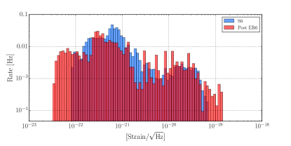
Figure 12 shows a comparison of LIGO Livingston’s detector data from S6 and from a lock stretch in March 2015 (Post ER6). Figure 12a compares the Omicron trigger rates binned by strain/ $\sqrt{\mathrm{Hz}}$ . It is clear to see that the triggers produced using Post ER6 data have a lower floor in strain/ $\sqrt{\mathrm{Hz}}$ than in S6 ( $<10^{-22}$ ) and the rate of glitches is generally lower across the entire amplitude range. The higher amplitude glitches ( $\sim 10^{-19}$ ) in the aLIGO data seem to be caused by the band of glitches around 500 and 1000 Hz, depicted in figure 12b. These are the fundamental and first harmonic of the test mass violin modes (as previously mentioned). For S6, these modes were closer to 340 and 680 Hz [1]. It is worth noting that the violin modes in aLIGO have a much higher Q than in Initial LIGO, hence they are more easily excited to super-thermal levels [3]. Figure 12b compares the triggers seen in both S6 and Post ER6 in terms of their frequency and amplitude. This plot highlights some of the most problematic regions to a transient search, in the frequency spectrum. Figures 12c and 12d show the rate of triggers, separated into four SNR bins over five minute intervals for the S6 and Post ER6 data respectively. Overall, the rate of triggers was less in the aLIGO March data compared to S6; the real difference can be seen in the rate of higher SNR triggers. Despite the variability of the aLIGO data (instrumental features at $\sim$ 1.5 and 5.5 hours in Figure 12d cause the glitch rate to increase), the glitch rate in certain SNR bins (SNR 8 - 20) is half to an order of magnitude lower in the March 2015 data than it was in 2010 (i.e. S6).

6 Concluding remarks

The Advanced LIGO detectors have been completely assembled and are currently being optimized to begin operation later this year, in what will be the most sensitive search for gravitational waves to date. In addition to maximizing the inspiral range, and therefore the volume over which an astrophysical search is conducted, it is just as important to ensure the data are as Gaussian and stationary as possible. In the last science run of initial LIGO (S6), many issues were identified as detrimental to a search for gravitational waves and harmful to the stability of the interferometers. Improvements were made in that some sources of noise were fixed at the instrument, but DQ flags were often used to identify known correlations between noise in an auxiliary channel and the gravitational wave channel [10]. For aLIGO, the hope is to identify and resolve harmful sources of noise as much as possible before an analysis is performed.

There have been many improvements to the aLIGO detectors during their commissioning phase; many issues have been identified and resolved at the source and this work continues. Section 5.1 highlights the improved quality of the detector data during this commissioning period, with the rate of glitches decreasing over the period studied. These same data were also compared with those from the last science run. The rate of glitches is less now than that seen in the last science run (Section 5.2). This work focused on data from the LIGO-Livingston detector and similar work is underway at LIGO-Hanford which will be presented in a future publication.

Over the coming months more effort will be made to further improve the output of the detectors to provide the best possible quality data to search for gravitational waves. Early efforts have already proven to be vital.

7 Acknowledgements

The authors would like to thank Gabriela González, Peter Saulson and David Shoemaker for useful discussions throughout the writing of this paper. LKN was supported by the College of Arts and Sciences at Syracuse University, TJM and RPF were supported by NSF award PHY-1205835 and DMM by NSF award PHY-1104371. JRS was supported by NSF CAREER 1255650. ARW was supported by the UK Science and Technology Facilities Council through grants ST/K501931/1 and ST/L000962/1. Some calculations were performed on the ORCA cluster supported by NSF award PHY-1429873. LIGO was constructed by the California Institute of Technology and Massachusetts Institute of Technology with funding from the National Science Foundation, and operates under cooperative agreement PHY-0757058. Advanced LIGO was built under award PHY-0823459. This paper has the LIGO Document Number LIGO-P1500131.

8 References

References

[1] B. P. Abbott et al. LIGO: The Laser Interferometer Gravitational-Wave Observatory. Rep. Prog. Phys, 72:076901, 2009.
[2] T. T. Fricke et al. DC Readout Experiment in Enhanced LIGO. Class. Quantum Grav., 79:065005, 2012.
[3] J. Aasi et al. Advanced LIGO. Class. Quantum Grav., 32:074001, 2015.
[4] J. Aasi et al. Prospects for Localization of Gravitational Wave Transients by the Advanced LIGO and Advanced Virgo Observatories. arXiv:1304.0670, 2013.
[5] J. Abadie et al. Predictions for the Rates of Compact Binary Coalescences Observable by Ground-Based Gravitational-Wave Detectors. Class. Quantum Grav., 27:173001, 2010.
[6] S. Klimenko et al. A Coherent Method for Detection of Gravitational Wave Bursts. Class. Quantum Grav., 25:114029, 2008.
[7] P. J. Sutton et al. X-Pipeline: An Analysis Package for Autonomous Gravitational-Wave Burst Searches. New J. Phys., 12:053034, 2010.
[8] I. W. Harry and S. Fairhurst. A Targeted Coherent Search for Gravitational Waves from Compact Binary Coalescences. Phys. Rev D, 83:084002, 2011.
[9] S. Babak et al. Searching for Gravitational Waves from Binary Coalescence. Phys. Rev D, 87:024033, 2013.
[10] J. Aasi et al. Characterization of the LIGO Detectors During their Sixth Science Run. Class. Quantum Grav., 32:115012, 2015.
[11] J. R. Smith. The Path to the Enhanced and Advanced LIGO Gravitational-Wave Detectors. Class. Quantum. Grav., 26:114013, 2009.
[12] N. Smith-Lefebvre et al. Optimal Alignment Sensing of a Readout Mode Cleaner Cavity. Optics Letters, 36:22:4365–4367, 2011.
[13] P. Kwee et al. Stablized High-Power Laser System for the Gravitational Wave Detector Advanced LIGO. Optics Express, 20(10):10617–10634, 2012.
[14] B. J. Meers. Recycling in Laser-Interferometric Gravitational-Wave Detectors. Phys. Rev. D., 38:2317, 1988.
[15] G. M. Harry et al. Thermal Noise from Optical Coatings in Gravitational Wave Detectors. Applied Optics, 45:7:1569–1574, 2006.
[16] G. M. Harry et al. Titania-Doped Tantala/Silica Coatings for Gravitational-Wave Detection. Class. Quantum. Grav., 24:405, 2007.
[17] M. Cavaglià and G. González. LSC Orgchart. LIGO-M1200248, 2015.
[18] D. M. Macleod et al. LHO Summary Pages. Internal Link: https://ldas-jobs.ligo-wa.caltech.edu/ detchar/summary/, 2014.
[19] D. M. Macleod et al. LLO Summary Pages. Internal Link: https://ldas-jobs.ligo-la.caltech.edu/ detchar/summary/, 2014.
[20] F. Robinet. Omicron: An Algorithm to Detect and Characterize Transient Noise in Gravitational-Wave Detectors. https://tds.ego-gw.it/ql/?c=10651, 2015.
[21] S. K. Chatterji. The Search for Gravitational Wave Bursts in Data from the Second LIGO Science Run. PhD Thesis: Massachusetts Institute of Technology, 2005.
[22] J. R. Smith et al. A Hierarchical Method for Vetoing Noise Transients in Gravitational-Wave Detectors. Class. Quantum Grav., 28:235005, 2011.
[23] S. Ballmer et al. Online Detector Characterization System Overview. Internal Document: LIGO-T1200323, 2013.
[24] General Standards Corportation. PMC66-18AO8 Reference Manual. http://www.generalstandards.com/user-manuals/pmc66_18ao8_man_092410.pdf, 092410:48, 2010.
[25] J. Betzwieser. DAC Glitches. LIGO-T1400649, 2014.
[26] I. Angert and D. Sigg. Characterization of a Voltage Controlled Oscillator. LIGO-T0900451, 2009.
[27] J. Abadie et al. Search for Gravitational Waves from the Low Mass Compact Binary Coalescence in LIGO’s Sixth Science Run and Virgo’s Science Runs 2 and 3. Phys Rev D, 85:082002, 2012.
[28] J. Abadie et al. All-Sky Search for Gravitational Waves Bursts in the Second Joint LIGO-Virgo Run. Phys Rev D, 85:122007, 2012.
[29] J. Aasi et al. Gravitational Waves from Known Pulsars: Results from the Initial Detector Era. ApJ, 785:119, 2014.