The LIGO Scientific Collaboration Instrument Science Authors

Improving astrophysical parameter estimation via offline noise subtraction for Advanced LIGO

J. C. Driggers LIGO Hanford Observatory, Richland, WA 99352, USA S. Vitale LIGO, Massachusetts Institute of Technology, Cambridge, MA 02139, USA A. P. Lundgren Max Planck Institute for Gravitational Physics (Albert Einstein Institute), D-30167 Hannover, Germany M. Evans LIGO, Massachusetts Institute of Technology, Cambridge, MA 02139, USA K. Kawabe LIGO Hanford Observatory, Richland, WA 99352, USA S. E. Dwyer LIGO Hanford Observatory, Richland, WA 99352, USA K. Izumi LIGO Hanford Observatory, Richland, WA 99352, USA R. M. S. Schofield University of Oregon, Eugene, OR 97403, USA A. Effler LIGO Livingston Observatory, Livingston, LA 70754, USA D. Sigg LIGO Hanford Observatory, Richland, WA 99352, USA P. Fritschel LIGO, Massachusetts Institute of Technology, Cambridge, MA 02139, USA M. Drago Max Planck Institute for Gravitational Physics (Albert Einstein Institute), D-30167 Hannover, Germany A. Nitz Max Planck Institute for Gravitational Physics (Albert Einstein Institute), D-30167 Hannover, Germany B. P. Abbott LIGO, California Institute of Technology, Pasadena, CA 91125, USA R. Abbott LIGO, California Institute of Technology, Pasadena, CA 91125, USA T. D. Abbott Louisiana State University, Baton Rouge, LA 70803, USA C. Adams LIGO Livingston Observatory, Livingston, LA 70754, USA R. X. Adhikari LIGO, California Institute of Technology, Pasadena, CA 91125, USA V. B. Adya Max Planck Institute for Gravitational Physics (Albert Einstein Institute), D-30167 Hannover, Germany A. Ananyeva LIGO, California Institute of Technology, Pasadena, CA 91125, USA S. Appert LIGO, California Institute of Technology, Pasadena, CA 91125, USA K. Arai LIGO, California Institute of Technology, Pasadena, CA 91125, USA S. M. Aston LIGO Livingston Observatory, Livingston, LA 70754, USA C. Austin Louisiana State University, Baton Rouge, LA 70803, USA S. W. Ballmer Syracuse University, Syracuse, NY 13244, USA D. Barker LIGO Hanford Observatory, Richland, WA 99352, USA B. Barr SUPA, University of Glasgow, Glasgow G12 8QQ, United Kingdom L. Barsotti LIGO, Massachusetts Institute of Technology, Cambridge, MA 02139, USA J. Bartlett LIGO Hanford Observatory, Richland, WA 99352, USA I. Bartos University of Florida, Gainesville, FL 32611, USA J. C. Batch LIGO Hanford Observatory, Richland, WA 99352, USA A. S. Bell SUPA, University of Glasgow, Glasgow G12 8QQ, United Kingdom J. Betzwieser LIGO Livingston Observatory, Livingston, LA 70754, USA G. Billingsley LIGO, California Institute of Technology, Pasadena, CA 91125, USA J. Birch LIGO Livingston Observatory, Livingston, LA 70754, USA S. Biscans LIGO, Massachusetts Institute of Technology, Cambridge, MA 02139, USA C. D. Blair LIGO Livingston Observatory, Livingston, LA 70754, USA R. M. Blair LIGO Hanford Observatory, Richland, WA 99352, USA R. Bork LIGO, California Institute of Technology, Pasadena, CA 91125, USA A. F. Brooks LIGO, California Institute of Technology, Pasadena, CA 91125, USA H. Cao OzGrav, University of Adelaide, Adelaide, South Australia 5005, Australia G. Ciani University of Florida, Gainesville, FL 32611, USA F. Clara LIGO Hanford Observatory, Richland, WA 99352, USA S. J. Cooper University of Birmingham, Birmingham B15 2TT, United Kingdom P. Corban LIGO Livingston Observatory, Livingston, LA 70754, USA S. T. Countryman Columbia University, New York, NY 10027, USA P. B. Covas Universitat de les Illes Balears, IAC3—IEEC, E-07122 Palma de Mallorca, Spain M. J. Cowart LIGO Livingston Observatory, Livingston, LA 70754, USA D. C. Coyne LIGO, California Institute of Technology, Pasadena, CA 91125, USA A. Cumming SUPA, University of Glasgow, Glasgow G12 8QQ, United Kingdom L. Cunningham SUPA, University of Glasgow, Glasgow G12 8QQ, United Kingdom K. Danzmann Max Planck Institute for Gravitational Physics (Albert Einstein Institute), D-30167 Hannover, Germany Leibniz Universität Hannover, D-30167 Hannover, Germany C. F. Da Silva Costa University of Florida, Gainesville, FL 32611, USA E. J. Daw The University of Sheffield, Sheffield S10 2TN, United Kingdom D. DeBra Stanford University, Stanford, CA 94305, USA R. DeSalvo California State University, Los Angeles, 5151 State University Dr, Los Angeles, CA 90032, USA K. L. Dooley Cardiff University, Cardiff CF24 3AA, United Kingdom The University of Mississippi, University, MS 38677, USA S. Doravari Max Planck Institute for Gravitational Physics (Albert Einstein Institute), D-30167 Hannover, Germany Leibniz Universität Hannover, D-30167 Hannover, Germany T. B. Edo The University of Sheffield, Sheffield S10 2TN, United Kingdom T. Etzel LIGO, California Institute of Technology, Pasadena, CA 91125, USA T. M. Evans LIGO Livingston Observatory, Livingston, LA 70754, USA H. Fair Syracuse University, Syracuse, NY 13244, USA A. Fernandez-Galiana LIGO, Massachusetts Institute of Technology, Cambridge, MA 02139, USA E. C. Ferreira Instituto Nacional de Pesquisas Espaciais, 12227-010 São José dos Campos, São Paulo, Brazil R. P. Fisher Syracuse University, Syracuse, NY 13244, USA H. Fong Canadian Institute for Theoretical Astrophysics, University of Toronto, Toronto, Ontario M5S 3H8, Canada R. Frey University of Oregon, Eugene, OR 97403, USA V. V. Frolov LIGO Livingston Observatory, Livingston, LA 70754, USA P. Fulda University of Florida, Gainesville, FL 32611, USA M. Fyffe LIGO Livingston Observatory, Livingston, LA 70754, USA B. Gateley LIGO Hanford Observatory, Richland, WA 99352, USA J. A. Giaime Louisiana State University, Baton Rouge, LA 70803, USA LIGO Livingston Observatory, Livingston, LA 70754, USA K. D. Giardina LIGO Livingston Observatory, Livingston, LA 70754, USA E. Goetz LIGO Hanford Observatory, Richland, WA 99352, USA R. Goetz University of Florida, Gainesville, FL 32611, USA S. Gras LIGO, Massachusetts Institute of Technology, Cambridge, MA 02139, USA C. Gray LIGO Hanford Observatory, Richland, WA 99352, USA H. Grote Cardiff University, Cardiff CF24 3AA, United Kingdom K. E. Gushwa LIGO, California Institute of Technology, Pasadena, CA 91125, USA E. K. Gustafson LIGO, California Institute of Technology, Pasadena, CA 91125, USA R. Gustafson University of Michigan, Ann Arbor, MI 48109, USA E. D. Hall LIGO, Massachusetts Institute of Technology, Cambridge, MA 02139, USA G. Hammond SUPA, University of Glasgow, Glasgow G12 8QQ, United Kingdom J. Hanks LIGO Hanford Observatory, Richland, WA 99352, USA J. Hanson LIGO Livingston Observatory, Livingston, LA 70754, USA T. Hardwick Louisiana State University, Baton Rouge, LA 70803, USA G. M. Harry American University, Washington, D.C. 20016, USA M. C. Heintze LIGO Livingston Observatory, Livingston, LA 70754, USA A. W. Heptonstall LIGO, California Institute of Technology, Pasadena, CA 91125, USA J. Hough SUPA, University of Glasgow, Glasgow G12 8QQ, United Kingdom R. Jones SUPA, University of Glasgow, Glasgow G12 8QQ, United Kingdom S. Kandhasamy LIGO Livingston Observatory, Livingston, LA 70754, USA S. Karki University of Oregon, Eugene, OR 97403, USA M. Kasprzack Louisiana State University, Baton Rouge, LA 70803, USA S. Kaufer Max Planck Institute for Gravitational Physics (Albert Einstein Institute), D-30167 Hannover, Germany Leibniz Universität Hannover, D-30167 Hannover, Germany R. Kennedy The University of Sheffield, Sheffield S10 2TN, United Kingdom N. Kijbunchoo OzGrav, Australian National University, Canberra, Australian Capital Territory 0200, Australia W. Kim OzGrav, University of Adelaide, Adelaide, South Australia 5005, Australia E. J. King OzGrav, University of Adelaide, Adelaide, South Australia 5005, Australia P. J. King LIGO Hanford Observatory, Richland, WA 99352, USA J. S. Kissel LIGO Hanford Observatory, Richland, WA 99352, USA W. Z. Korth LIGO, California Institute of Technology, Pasadena, CA 91125, USA G. Kuehn Max Planck Institute for Gravitational Physics (Albert Einstein Institute), D-30167 Hannover, Germany Leibniz Universität Hannover, D-30167 Hannover, Germany M. Landry LIGO Hanford Observatory, Richland, WA 99352, USA B. Lantz Stanford University, Stanford, CA 94305, USA M. Laxen LIGO Livingston Observatory, Livingston, LA 70754, USA J. Liu OzGrav, University of Western Australia, Crawley, Western Australia 6009, Australia N. A. Lockerbie SUPA, University of Strathclyde, Glasgow G1 1XQ, United Kingdom M. Lormand LIGO Livingston Observatory, Livingston, LA 70754, USA M. MacInnis LIGO, Massachusetts Institute of Technology, Cambridge, MA 02139, USA D. M. Macleod Cardiff University, Cardiff CF24 3AA, United Kingdom S. Márka Columbia University, New York, NY 10027, USA Z. Márka Columbia University, New York, NY 10027, USA A. S. Markosyan Stanford University, Stanford, CA 94305, USA E. Maros LIGO, California Institute of Technology, Pasadena, CA 91125, USA P. Marsh University of Washington Bothell, 18115 Campus Way NE, Bothell, WA 98011, USA I. W. Martin SUPA, University of Glasgow, Glasgow G12 8QQ, United Kingdom D. V. Martynov LIGO, Massachusetts Institute of Technology, Cambridge, MA 02139, USA K. Mason LIGO, Massachusetts Institute of Technology, Cambridge, MA 02139, USA T. J. Massinger LIGO, California Institute of Technology, Pasadena, CA 91125, USA F. Matichard LIGO, California Institute of Technology, Pasadena, CA 91125, USA LIGO, Massachusetts Institute of Technology, Cambridge, MA 02139, USA N. Mavalvala LIGO, Massachusetts Institute of Technology, Cambridge, MA 02139, USA R. McCarthy LIGO Hanford Observatory, Richland, WA 99352, USA D. E. McClelland OzGrav, Australian National University, Canberra, Australian Capital Territory 0200, Australia S. McCormick LIGO Livingston Observatory, Livingston, LA 70754, USA L. McCuller LIGO, Massachusetts Institute of Technology, Cambridge, MA 02139, USA J. McIver LIGO, California Institute of Technology, Pasadena, CA 91125, USA D. J. McManus OzGrav, Australian National University, Canberra, Australian Capital Territory 0200, Australia T. McRae OzGrav, Australian National University, Canberra, Australian Capital Territory 0200, Australia G. Mendell LIGO Hanford Observatory, Richland, WA 99352, USA E. L. Merilh LIGO Hanford Observatory, Richland, WA 99352, USA P. M. Meyers University of Minnesota, Minneapolis, MN 55455, USA R. Mittleman LIGO, Massachusetts Institute of Technology, Cambridge, MA 02139, USA K. Mogushi The University of Mississippi, University, MS 38677, USA D. Moraru LIGO Hanford Observatory, Richland, WA 99352, USA G. Moreno LIGO Hanford Observatory, Richland, WA 99352, USA C. M. Mow-Lowry University of Birmingham, Birmingham B15 2TT, United Kingdom G. Mueller University of Florida, Gainesville, FL 32611, USA N. Mukund Inter-University Centre for Astronomy and Astrophysics, Pune 411007, India A. Mullavey LIGO Livingston Observatory, Livingston, LA 70754, USA J. Munch OzGrav, University of Adelaide, Adelaide, South Australia 5005, Australia T. J. N. Nelson LIGO Livingston Observatory, Livingston, LA 70754, USA P. Nguyen University of Oregon, Eugene, OR 97403, USA L. K. Nuttall Cardiff University, Cardiff CF24 3AA, United Kingdom J. Oberling LIGO Hanford Observatory, Richland, WA 99352, USA M. Oliver Universitat de les Illes Balears, IAC3—IEEC, E-07122 Palma de Mallorca, Spain P. Oppermann Max Planck Institute for Gravitational Physics (Albert Einstein Institute), D-30167 Hannover, Germany Leibniz Universität Hannover, D-30167 Hannover, Germany Richard J. Oram LIGO Livingston Observatory, Livingston, LA 70754, USA B. O’Reilly LIGO Livingston Observatory, Livingston, LA 70754, USA D. J. Ottaway OzGrav, University of Adelaide, Adelaide, South Australia 5005, Australia H. Overmier LIGO Livingston Observatory, Livingston, LA 70754, USA J. R. Palamos University of Oregon, Eugene, OR 97403, USA W. Parker LIGO Livingston Observatory, Livingston, LA 70754, USA A. Pele LIGO Livingston Observatory, Livingston, LA 70754, USA S. Penn Hobart and William Smith Colleges, Geneva, NY 14456, USA C. J. Perez LIGO Hanford Observatory, Richland, WA 99352, USA M. Phelps SUPA, University of Glasgow, Glasgow G12 8QQ, United Kingdom V. Pierro University of Sannio at Benevento, I-82100 Benevento, Italy and INFN, Sezione di Napoli, I-80100 Napoli, Italy I. M. Pinto University of Sannio at Benevento, I-82100 Benevento, Italy and INFN, Sezione di Napoli, I-80100 Napoli, Italy M. Pirello LIGO Hanford Observatory, Richland, WA 99352, USA M. Principe University of Sannio at Benevento, I-82100 Benevento, Italy and INFN, Sezione di Napoli, I-80100 Napoli, Italy L. G. Prokhorov Faculty of Physics, Lomonosov Moscow State University, Moscow 119991, Russia O. Puncken Max Planck Institute for Gravitational Physics (Albert Einstein Institute), D-30167 Hannover, Germany Leibniz Universität Hannover, D-30167 Hannover, Germany V. Quetschke The University of Texas Rio Grande Valley, Brownsville, TX 78520, USA E. A. Quintero LIGO, California Institute of Technology, Pasadena, CA 91125, USA H. Radkins LIGO Hanford Observatory, Richland, WA 99352, USA P. Raffai Institute of Physics, Eötvös University, Pázmány P. s. 1/A, Budapest 1117, Hungary K. E. Ramirez The University of Texas Rio Grande Valley, Brownsville, TX 78520, USA S. Reid SUPA, University of Strathclyde, Glasgow G1 1XQ, United Kingdom D. H. Reitze LIGO, California Institute of Technology, Pasadena, CA 91125, USA University of Florida, Gainesville, FL 32611, USA N. A. Robertson LIGO, California Institute of Technology, Pasadena, CA 91125, USA SUPA, University of Glasgow, Glasgow G12 8QQ, United Kingdom J. G. Rollins LIGO, California Institute of Technology, Pasadena, CA 91125, USA V. J. Roma University of Oregon, Eugene, OR 97403, USA C. L. Romel LIGO Hanford Observatory, Richland, WA 99352, USA J. H. Romie LIGO Livingston Observatory, Livingston, LA 70754, USA M. P. Ross University of Washington, Seattle, WA 98195, USA S. Rowan SUPA, University of Glasgow, Glasgow G12 8QQ, United Kingdom K. Ryan LIGO Hanford Observatory, Richland, WA 99352, USA T. Sadecki LIGO Hanford Observatory, Richland, WA 99352, USA E. J. Sanchez LIGO, California Institute of Technology, Pasadena, CA 91125, USA L. E. Sanchez LIGO, California Institute of Technology, Pasadena, CA 91125, USA V. Sandberg LIGO Hanford Observatory, Richland, WA 99352, USA R. L. Savage LIGO Hanford Observatory, Richland, WA 99352, USA D. Sellers LIGO Livingston Observatory, Livingston, LA 70754, USA D. A. Shaddock OzGrav, Australian National University, Canberra, Australian Capital Territory 0200, Australia T. J. Shaffer LIGO Hanford Observatory, Richland, WA 99352, USA B. Shapiro Stanford University, Stanford, CA 94305, USA D. H. Shoemaker LIGO, Massachusetts Institute of Technology, Cambridge, MA 02139, USA B. J. J. Slagmolen OzGrav, Australian National University, Canberra, Australian Capital Territory 0200, Australia B. Smith LIGO Livingston Observatory, Livingston, LA 70754, USA J. R. Smith California State University Fullerton, Fullerton, CA 92831, USA B. Sorazu SUPA, University of Glasgow, Glasgow G12 8QQ, United Kingdom A. P. Spencer SUPA, University of Glasgow, Glasgow G12 8QQ, United Kingdom K. A. Strain SUPA, University of Glasgow, Glasgow G12 8QQ, United Kingdom D. B. Tanner University of Florida, Gainesville, FL 32611, USA R. Taylor LIGO, California Institute of Technology, Pasadena, CA 91125, USA M. Thomas LIGO Livingston Observatory, Livingston, LA 70754, USA P. Thomas LIGO Hanford Observatory, Richland, WA 99352, USA K. A. Thorne LIGO Livingston Observatory, Livingston, LA 70754, USA E. Thrane OzGrav, School of Physics & Astronomy, Monash University, Clayton 3800, Victoria, Australia K. Toland SUPA, University of Glasgow, Glasgow G12 8QQ, United Kingdom C. I. Torrie LIGO, California Institute of Technology, Pasadena, CA 91125, USA G. Traylor LIGO Livingston Observatory, Livingston, LA 70754, USA M. Tse LIGO, Massachusetts Institute of Technology, Cambridge, MA 02139, USA D. Tuyenbayev The University of Texas Rio Grande Valley, Brownsville, TX 78520, USA G. Vajente LIGO, California Institute of Technology, Pasadena, CA 91125, USA G. Valdes Louisiana State University, Baton Rouge, LA 70803, USA A. A. van Veggel SUPA, University of Glasgow, Glasgow G12 8QQ, United Kingdom S. Vass LIGO, California Institute of Technology, Pasadena, CA 91125, USA A. Vecchio University of Birmingham, Birmingham B15 2TT, United Kingdom P. J. Veitch OzGrav, University of Adelaide, Adelaide, South Australia 5005, Australia K. Venkateswara University of Washington, Seattle, WA 98195, USA G. Venugopalan LIGO, California Institute of Technology, Pasadena, CA 91125, USA T. Vo Syracuse University, Syracuse, NY 13244, USA C. Vorvick LIGO Hanford Observatory, Richland, WA 99352, USA M. Walker California State University Fullerton, Fullerton, CA 92831, USA R. L. Ward OzGrav, Australian National University, Canberra, Australian Capital Territory 0200, Australia J. Warner LIGO Hanford Observatory, Richland, WA 99352, USA B. Weaver LIGO Hanford Observatory, Richland, WA 99352, USA R. Weiss LIGO, Massachusetts Institute of Technology, Cambridge, MA 02139, USA P. Weßels Max Planck Institute for Gravitational Physics (Albert Einstein Institute), D-30167 Hannover, Germany Leibniz Universität Hannover, D-30167 Hannover, Germany B. Willke Max Planck Institute for Gravitational Physics (Albert Einstein Institute), D-30167 Hannover, Germany Leibniz Universität Hannover, D-30167 Hannover, Germany C. C. Wipf LIGO, California Institute of Technology, Pasadena, CA 91125, USA J. Worden LIGO Hanford Observatory, Richland, WA 99352, USA H. Yamamoto LIGO, California Institute of Technology, Pasadena, CA 91125, USA C. C. Yancey University of Maryland, College Park, MD 20742, USA Hang Yu LIGO, Massachusetts Institute of Technology, Cambridge, MA 02139, USA Haocun Yu LIGO, Massachusetts Institute of Technology, Cambridge, MA 02139, USA L. Zhang LIGO, California Institute of Technology, Pasadena, CA 91125, USA M. E. Zucker LIGO, Massachusetts Institute of Technology, Cambridge, MA 02139, USA LIGO, California Institute of Technology, Pasadena, CA 91125, USA J. Zweizig LIGO, California Institute of Technology, Pasadena, CA 91125, USA

Abstract

The Advanced LIGO detectors have recently completed their second observation run successfully. The run lasted for approximately 10 months and lead to multiple new discoveries. The sensitivity to gravitational waves was partially limited by correlated noise. Here, we utilize auxiliary sensors that witness these correlated noise sources, and use them for noise subtraction in the time domain data. This noise and line removal is particularly significant for the LIGO Hanford Observatory, where the improvement in sensitivity is greater than 20%. Consequently, we were also able to improve the astrophysical estimation for the location, masses, spins and orbital parameters of the gravitational wave progenitors.

pacs:

04.30.-w, 04.80.Nn, 95.55.Ym, 04.25.dg, 04.25.dk

I Introduction

Advanced LIGO’s Aasi et al. (2015) detections of gravitational waves Abbott et al. (2016, 2017, 2017, 2016, 2017, 2017, ) have opened up a new view of the universe, allowing us to learn about astrophysical sources such as the mergers of compact stellar remnants. As work continues toward reaching the design sensitivity of Advanced LIGO, we are looking forward to more detections of gravitational waves (GW), and learning more about their sources Abbott et al. ; Abbott et al. (2016).

The Advanced LIGO detectors are kilometer-scale laser interferometers with suspended test masses, sophisticated seismic isolation systems and complex optical configurations employing multiple coupled optical resonators Abbott et al. (2016). LIGO’s design sensitivity is limited primarily by fundamental noise sources such as quantum shot noise, quantum radiation pressure noise, and Brownian thermal noise. However, in some frequency bands, Advanced LIGO’s first observation runs have been limited by technical noises Martynov et al. (2016); Abbott et al. . Many of these noise sources are well understood, and further work is needed to prevent them from contaminating the gravitational wave sensitivity. In practice, a balance has to be struck between commissioning the detector to improve noise performance, and observations. For the second observation run from November 2016 to August 2017, the LIGO Scientific Collaboration elected to run with somewhat elevated noise in one of the interferometers, while making plans to address these noise sources prior to the third observation run.

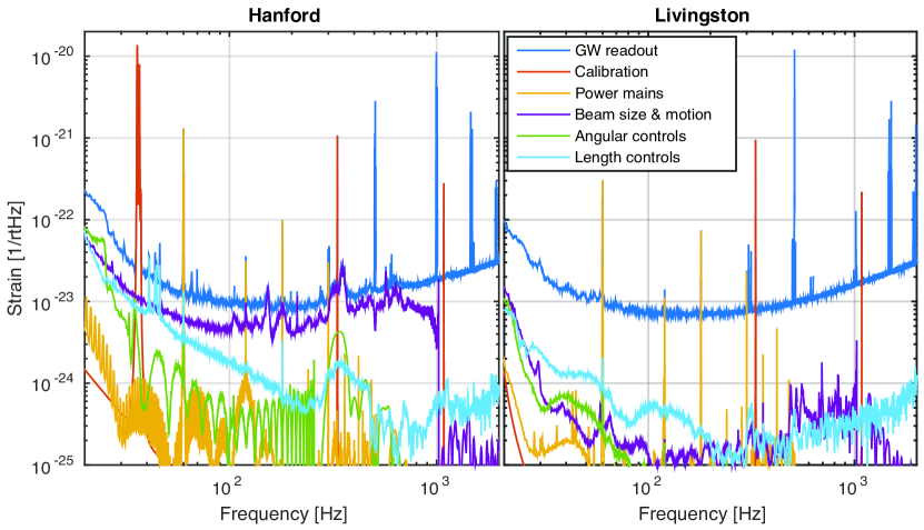
The sensitivity of the LIGO Hanford detector is severely affected by laser noise in the frequency band from 100 Hz to 1 kHz. Fortunately, we have a set of independent witness sensors that is highly correlated with this noise. The spectra of both detectors also reveal the power mains and its harmonics, as well as lines that are monitoring the calibration in realtime. Noise and line removal can enhance the sensitivity of the LIGO Hanford detector by more than 20 % during the second observing run. By implementing a post-processing noise removal algorithm, we are able to significantly improve our ability to estimate the parameters of a compact binary coalescence, including its sky location, distance, masses, spins and orbital mechanics.

The removal of lines with narrow frequency spread is also beneficial in the search for continuous wave sources, such as spinning neutron stars. Due to the long signal duration, the frequency of the observed gravitational wave signals are Doppler shifted by the rotation of the earth and the motion of the earth around the sun. Narrow spectral lines are broadened after the Doppler effect has been removed, and can therefore impact a wider frequency band. Currently, the continuous wave searches ignore a relatively wide frequency gap around each spectral line to account for this. The search for continuous waves is fundamentally a post processing algorithm and can naturally benefit from any sensitivity improvements made in our post-processing noise and line removal technique.

Section II briefly describes the origin of several noise sources that can be removed, while Section III discusses the available witness sensors and the method for calculating the coupling functions used in the subtraction algorithm. Section IV examines how this post-processing noise subtraction impacts the estimation of various astrophysical parameters.

II Technical noise sources

After the first Advanced LIGO observing run, lasting from September 2015 to January 2016, the two LIGO observatories in Hanford, Washington, and Livingston, Louisiana, underwent a series of upgrades Abbott et al. . The Handford observatory focused on increasing the amount of laser power circulating in the interferometer, which required using a high power oscillator Kwee et al. (2012). The water required for cooling the laser rods flows through piping attached to the laser table, causing vibrations. This table also hosts an optical train for shaping the beam, impressing radio frequency sidebands, beam steering, and frequency stabilization. The water flow causes vibrations of these optical elements, which translates into beam jitter. Thermal fluctuations in the laser rods and mode mismatch in the optical resonators are also causing jitter variations of the the laser beam size—likely due to the turbulent water flow directly over the laser rods Schofield .

During Advanced LIGO’s second observing run, it was discovered that one of the core mirrors in the long arm cavities at the Hanford observatory sports a point absorber on its surface. Depending on the incident power, this causes a beam deformation due to the thermal expansion of the optics and the temperature dependence of the index of refraction. LIGO has a thermally actuated adaptive optics system Brooks et al. (2016) to help compensate for effects that are axially symmetric about the beam axis, but which cannot remove the effect of a point absorber that is located several millimeter away from the center.

The presence of this non-asymmetric optical deformation couples beam jitter and beam size variations into the gravitational wave readout channel. During the run, an attempt was made to inspect the offending mirror and try to clean off the absorption spot. But, this failed with the cleaning having no appreciable effect on the absorption, and so this optic has been replaced prior to the start of the third observing run. As a result, the higher beam jitter and beam size variations significantly impacted the gravitational wave readout sensitivity of the LIGO Hanford Observatory during the entire second observation run.

The LIGO Livingston Observatory did not utilize their high power laser oscillator during the second observation run, and so required much less cooling water to flow through the piping on the laser table. Instead, the commissioning effort at the Livingston Observatory focused on finding and mitigating various noise sources, such as scattered light and coupling of electronics noise. This complementary approach in the commissioning of the two LIGO detectors is common, and enables early experience with new hardware configurations. Both interferometers are susceptible to the power mains that show up in the gravitational wave readout. An active set of calibration lines is used to track the variations in the optical gain. Both the power mains and the calibration line are well known, and therefore can be subtracted from the measured gravitational wave strain.

At frequencies below a few tens of Hertz, additional noise is introduced by the control forces that are applied to the mirrors to control the resonance condition of the interferometer and the test mass orientation. In addition to the 4 km long arm cavities, the LIGO detectors have optical cavities in the central part of the interferometer whose lengths must be controlled to keep the interferometer at its linear operating point. The sensors used for the auxiliary length degrees of freedom have worse shot noise limited sensitivity than the gravitational wave readout channel. Since this shot noise is imposed on the actual length noise of the auxiliary cavities by our feedback controls, it can contaminate the gravitational wave readout channel. The feedback control system actively tries to decouple two of the three length degrees of freedom from the gravitational wave readout channel. But, due to a remaining imbalance in the actuator strength and due to leaving the third degree of freedom untouched, some noise still couples into the gravitational wave readout channel. This noise can also be removed in post-processing.

Figure 1 shows the noise amplitude spectral density (ASD) of the LIGO detectors in the low-latency readout, and estimates the noise contributions from each of the categories described above.

Refer to caption — Figure 1: Noise amplitude spectral density of the Advanced LIGO detectors (dark blue) with the left panel for Hanford and the right panel for Livingston. The other traces are the estimated contributions of the calibration lines (red), power line and harmonics (gold), beam jitter motion and beam size variations (purple), angular control noise (green), and the auxiliary length controls degree of freedom (light blue). These spectra are based on 1024 s of data starting on 25 June 2017 at 08:00:00 UTC, at a time when both LIGO interferometers were operating and in an observation ready state.

III Noise subtraction

We use the optimal Wiener method Wiener (1964) to estimate the coupling function between each noise source and the GW channel. This method determines how best to manipulate an auxiliary witness sensor’s data such that when it is subtracted from the primary target signal (here, the GW channel) the mean-square-error of the primary channel is minimized. To do this, we define an error signal

\vec{e}=\vec{d}-\vec{y},

(1)

where $\vec{d}$ is the noisy target signal and $\vec{y}$ is the approximation of $\vec{d}$ from the independent witness sensor. This is given by

\vec{y}=\vec{w}^{\rm T}\vec{x},

(2)

where $\vec{x}$ is the measurement of the external disturbance from the witness sensor, and $\vec{w}$ is the finite impulse response (FIR) filter that we will solve for. The figure of merit $(\xi)$ that we use for calculating the Wiener filter coefficients in this case is the expectation value of the square of the error signal,

\xi\equiv E[\vec{e}\,^{2}]=E[\vec{d}\ ^{2}]-2\vec{w}^{\textrm{T}}\vec{p}+\vec{w}^{\textrm{T}}R\vec{w}.

(3)

Here, $E[*]$ indicates the expectation value of $*$ , $\vec{p}$ is the cross-correlation vector between the witness and target signals, and $R$ is the autocorrelation matrix for the witness channels. When we find the extrema of Equation 3 by setting

\frac{d\xi}{dw_{i}}=0,

(4)

we find

R\vec{w}_{\rm optimum}=\vec{p}.

(5)

Equation 5 finds the time domain filter coefficients which minimize the RMS of the error $\vec{e}$ by optimizing the estimate of the transfer function between the witness sensors and the target signal. The error signal is now an estimate of the signal in $\vec{d}$ , without any noise.

This method was utilized on LIGO data in 2010, for low frequency seismic noise Driggers et al. (2012). Following this, the method was used to create feed forward filters which were used online in 2010 DeRosa et al. (2012). This and another method were also used offline to remove noise from auxiliary degrees of freedom from LIGO’s initial-era sixth science run Meadors et al. (2014); Tiwari et al. (2015). A frequency-dependent variant of noise subtraction was proposed in 1999 Allen et al. (1999), and shown to be effective on a prototype interferometer’s data.

The Wiener method is able to handle several witness sensors simultaneously by extending $R$ and $\vec{p}$ in the above equations, even if they see some amount of signal from the same noise source, as long as the information in the auxiliary sensors is not identical. This prevents over-subtracting a source of noise, and eliminates the need to carefully chose the order of subtraction if the witness sensors are used in series. The inversion of the matrix ( $R^{-1}$ when Equation 5 is solved for $\vec{w}_{\rm optimum}$ ) is computationally intensive, and is the main time-limiting step in the noise removal process.

As this method works to minimize the root mean square (RMS) of the target channel, it is useful to remove narrow spectral lines from the data before attempting to subtract the broadband noise sources. For the calibration lines we use the digital signals that are sent to the various actuators as our auxiliary channels. Since we know that these signals sent to different actuators are not correlated with one another, we subtract them in series. For the power mains line at 60 Hz we use a digitized signal that comes directly from monitoring the voltage supplied to our analog electronics racks. While we monitor the voltage at all locations that host analog electronics for the interferometer, we empirically chose the one signal at each site that removes most of the 60 Hz line. In the future, we may consider utilizing more of these signals, particularly for subtraction over longer periods of time.

To measure the beam jitter motion we use a set of three split photodiodes, each with four sections. One of the photodiodes is placed on the laser table, and monitors the beam motion and beam size just after the laser itself. This diode has a central circle, and a ring of three equal-sized segments surrounding the central region. The other two split photodetectors monitor the vertical and horizontal motion of the beam rejected by the input mode cleaner cavity which spatially filters the laser beam before it enters the main interferometer. The signals from these photodiodes are all passed to the Wiener filter calculation algorithm together.

For both the angular and length control noise sources we use the digital control signals that are sent to the mirror actuators as the witnesses.

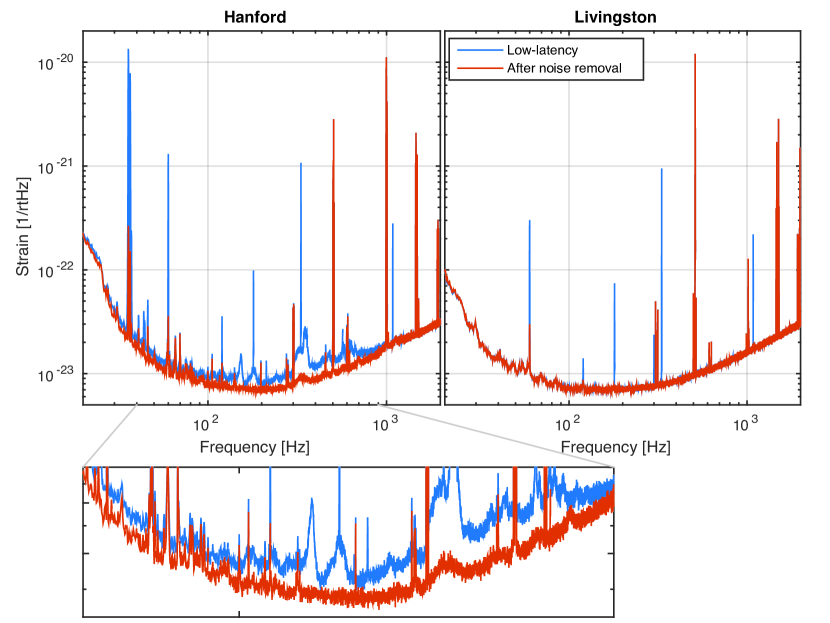
Figure 2 shows the improvement that can be made in the LIGO interferometers’ noise ASD, as a function of frequency. Note that the LIGO Hanford detector is compromised by the technical noise sources discussed above more significantly than is the LIGO Livingston detector, and so sees much more dramatic improvement. Notable spectral lines such as those at $\sim$ 500 Hz and harmonics cannot be independently witnessed with currently existing hardware, and so cannot be subtracted. The LIGO interferometers’ alignment can change slowly with time, which causes the coupling of some noise sources to change. Empirically, it seems that the coupling functions should be recalculated about once per hour of data. For all of the gravitational wave events that have utilized this method of post-processing noise subtraction (GW170608 Abbott et al. , GW170814 Abbott et al. (2017), and GW170817 Abbott et al. (2017)), the coupling functions were calculated using 1024 s of data, and applied to 4096 s of data surrounding each event.

A measure of the improvement in each interferometer can be summarized by the increase in horizon distance the detectors can see a certain GW signal with a pre-defined signal to noise ratio. For both canonical binary black hole $30\,M_{\odot}$ - $30\,M_{\odot}$ mergers as well as canonical neutron star $1.4\,M_{\odot}$ - $1.4\,M_{\odot}$ coalescences with a signal to noise ratio of 8 the Hanford detector improves by more than 20% while the Livingston interferometer only improves by about 0.5% using this measure.

Several checks can be done to confirm that this noise removal procedure does not affect any gravitational wave signal present in the data. Most of the noise sources have no possibility of containing any gravitational wave information, therefore cannot remove any actual signal. For example, the power mains monitors, calibration lines, and beam motion photodiodes do not contain any GW signal. For other witness sensors such as length of the short Michelson, we can calculate that the GW signal there is a factor of $1.2\times 10^{-5}$ smaller than in the main GW readout channel Driggers (2015); Meadors et al. (2014); Izumi and Sigg (2017), so should only impact the GW signal up to 0.0012%.

Perhaps the most robust way to check that there is no harm done to a GW signal is to examine software injected signals, where we know the true (simulated) parameters, and can compare the estimated parameters from the low-latency data and the post-processed noise-subtracted data. We do this in Section IV.

IV Estimation of astrophysical parameters

Improved interferometer sensitivity not only enhances our confidence that a signal is of astrophysical origin, but it greatly improves our ability to estimate astrophysical parameters associated with the source of the GWs.

To estimate quantitatively the impact of post-processing noise subtraction on the characterization of GW sources, we performed software injections of signals emitted from compact binary coalescences. By software injection one means a simulated GW signal which is added to either real or synthetic interferometric noise.

For this study, we created 10 binary black hole (BBH) signals and 9 binary neutron star (BNS) signals. For the BBH, we used the IMRPhenomPv2 waveform model, whereas for the BNS we used TaylorF2. This latter does not include merger and ringdown, which is a reasonable approximation at low masses. The BBH have component (detector-frame) masses randomly drawn from the range $[28-64]\,M_{\odot}$ , resulting in mass ratios ¹¹1We define the mass ratio $q\equiv m_{2}/m_{1}$ , where by convention $m_{1}\geq m_{2}$ . in the range $0.48-1.0$ . The BBH are injected with zero spin (although we do allow for the spins degrees of freedom while measuring the BBH parameters). The BNS have masses in the range $[1.41-1.45]\,M_{\odot}$ and no spins. The luminosity distance of the events random in comoving volume. In practice, this results in distances between 70 Mpc and 1.54 Gpc for the BBH and 14 Mpc and 138 Mpc for the BNS.

For each signal, we add it to a stretch of the LIGO Hanford and Livingston detectors data when both instruments were online and in a nominal observational state (1024 s beginning at 25 June 2017 08:00:00 UTC). For each signal and each instrument, a frame file (this is the file format commonly used within the LIGO-Virgo Collaboration to store GW data containing the signal and the original noise is created and saved. The cleaning procedure is then performed on all frame files, and new “cleaned” frames are stored. This leaves us with two sets of frame files: one with the original LIGO data (as well as the GW signal), and one with the cleaned data (and, again, the signal).

Both set of frames are analyzed with the same algorithm used by the LIGO and Virgo collaborations to characterize compact binary coalescence sources, LALInference Veitch et al. (2015). For each signal, we aim to obtain a posterior distribution for the unknown parameters on which it depends, $\vec{\theta}$ , given the stretch of data containing the i-th signal: $p(\vec{\theta}|d_{i})$ . Using Bayes’ theorem, this can be written:

p(\vec{\theta}|d_{i})\propto p(d_{i}|\vec{\theta})p(\vec{\theta}),

(6)

where the proportionality coefficient just acts as an overall normalization. The first term on the right hand side, $p(d_{i}|\vec{\theta})$ , is the likelihood of the data given the parameters. In this paper we work with a two-detector network. Assuming noise is statistically independent in the two instruments we can write the network likelihood as the product of the likelihood in each instrument:

p(d_{i}|\vec{\theta})=\prod_{k=1}^{\mathrm{N\;IFO}}p(d_{i}^{k}|\vec{\theta}).

(7)

Finally, $p(\vec{\theta})$ is the prior distribution of $\vec{\theta}$ . For this study we used the same priors already utilized by the LIGO and Virgo collaborations, see e.g. Ref. Abbott et al. (2016).

Most of the unknown parameters are common to both the BBH and the BNS analyses. These include component masses, luminosity distance, orbital inclination and polarization, sky position, arrival time, and phase Abbott et al. (2016). The only difference is that for the BNS analysis we assumed spins are aligned with the orbital angular momentum, while for the BBH we allowed for the possibility of misalignment, and hence precession. For the BBH runs, we relied on the reduced order quadrature approximation to the likelihood Smith et al. (2016) to reduce the runtime.

On average, we observe an increase of the signal-to-noise (SNR) at Hanford of $\sim 29\%$ for both BNS and BBH. This results on a $\sim 10\%$ increase in the network SNR. The improvement in the network SNR is less dramatic, since the SNRs at each interferometer are added in quadrature Veitch et al. (2015).

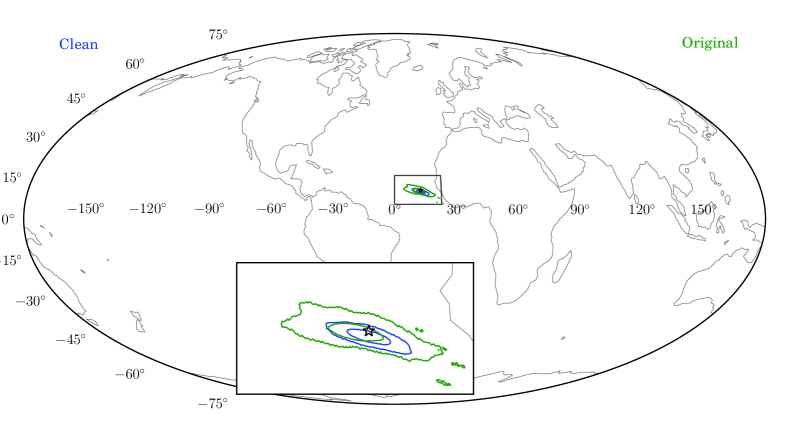
The increased SNR at Hanford yields a more balanced distribution of the SNR across the two sites, which mostly helps measuring the location of the source on the sky. For the BNS simulations, we find a $32.2\%$ reduction of the 90% credible interval in the sky localization, compared to what was obtained with the original uncleaned data. This is shown in Fig. 3 for the loudest BNS we simulated ²²2Most of the other events show similar improvements; we chose to show this one because for other sources the skymap has a characterizing ring-like structure, which does not allow one to clearly see the difference between the reconstructions. . The green curves refers to the analysis using the original data, whereas the blue curves are obtained with the cleaned data. 50% and 90% contours are given, and and star shows the true position. For this BNS, the 90% sky area decreases from 39.6 $\mathrm{deg}^{2}$ to 11.6 $\mathrm{deg}^{2}$ using cleaned data, while the SNR in Hanford increases from 25.5 to 33.0 (the network SNR increases from 65.0 to 68.5). For BBH, the average reduction of the 90% sky uncertainty is $19.5\%$ . The estimation of the sources’ luminosity distance is also improved, although not dramatically so, since its measurement requires detection of both GW’s polarizations, whereas the two LIGO sites have nearly aligned arms. Adding more SNR in Hanford thus does not add significant polarization information. We find an average improvement of $6.6\%$ for BNS and $2.0\%$ for BBH for luminosity distance.

The the intrinsic parameters of the sources, i.e. masses and spins, can usually be measured well already with a single instrument. The uncertainty in those quantities is thus mostly affected by the network SNR, and not so sensitive to how that SNR is distributed in the network. For the chirp mass Abbott et al. (2016) we find a relative improvement of $5.2\%$ for the BNS and $13.4\%$ for the BBH. The reason why BBH improve more is because they have fewer inspiral cycles (from which the chirp mass is measured Abbott et al. (2016)) than BNS. They can thus benefit more from any extra SNR at frequencies below $\sim 100$ Hz.

Similar small improvements are visible for the asymmetric mass ratio and the effective spin parameter $\chi_{\mathrm{eff}}$ Racine (2008); Abbott et al. (2016). We find that cleaning makes little difference in this case. For a few BNS sources the uncertainty is actually slightly smaller before cleaning. On average, the mass ratio is estimated $1.4\%$ worse when using cleaned data. For BBH, we also find a few sources for which the uncertainty is smaller before cleaning, although when averaging over all sources, cleaned data yield intervals which are $5.1\%$ better with cleaned data. For $\chi_{\mathrm{eff}}$ we find an average improvement of $8.5\%$ for BBH and $0.1\%$ for BNS.

V Conclusions

We have shown that post-processing noise subtraction is effective for the Advanced LIGO gravitational wave detectors, particularly for the Hanford Observatory during the second observation run which is limited by known technical noise sources over a wide range of frequencies. This sensitivity improvement significantly enhances our ability to extract astrophysical information from our detected signals. The improvement in sensitivity shown roughly doubles the volume of the universe in which the Hanford interferometer can detect gravitational waves. Currently underway is the rewriting of the noise subtraction code such that it is scalable and can be applied to the entirety of the data from the second observation run. This will allow the background estimations of events to also use cleaned data, and will enable the CW search to look at frequencies they have never been able to see before.

VI Acknowledgements

The authors would like to thank the LIGO Scientific Collaboration’s astrophysical parameter estimation group for their support. SV would like to thank R. Essick for providing the code to plot the sky location of sources. We are also very grateful for the computing support provided by The MathWorks, Inc. LIGO was constructed by the California Institute of Technology and Massachusetts Institute of Technology with funding from the National Science Foundation and operates under cooperative agreement PHY-0757058. This article has been given LIGO document number P1700260.

References

Aasi et al. (2015) J. Aasi et al. (LIGO Scientific Collaboration), Class. Quantum Grav., 32, 074001 (2015), arXiv:1411.4547 [gr-qc] .
Abbott et al. (2016) B. P. Abbott et al. (LIGO Scientific Collaboration and Virgo Collaboration), Phys. Rev. Lett., 116, 061102 (2016a), arXiv:1602.03837 [gr-qc] .
Abbott et al. (2017) B. P. Abbott et al. (LIGO Scientific Collaboration and Virgo Collaboration), Phys. Rev. Lett., 119, 161101 (2017a).
Abbott et al. (2017) B. P. Abbott et al., ApJ. Lett., 848, L12 (2017b).
Abbott et al. (2016) B. P. Abbott et al. (LIGO Scientific Collaboration and Virgo Collaboration), Phys. Rev. Lett., 116, 241103 (2016b), arXiv:1606.04855 [gr-qc] .
Abbott et al. (2017) B. P. Abbott et al. (LIGO Scientific Collaboration and Virgo Collaboration), Phys. Rev. Lett., 118, 221101 (2017c), arXiv:1706.01812 [gr-qc] .
Abbott et al. (2017) B. P. Abbott et al. (LIGO Scientific Collaboration and Virgo Collaboration), Phys. Rev. Lett., 119, 141101 (2017d).
(8) B. P. Abbott et al. (LIGO Scientific Collaboration and Virgo Collaboration), Ap. J. Lett., accepted (a).
(9) B. P. Abbott et al. ((KAGRA Collaboration, LIGO Scientific Collaboration and Virgo Collaboration), “Prospects for observing and localizing gravitational-wave transients with Advanced LIGO, Advanced Virgo and KAGRA,” https://dcc.ligo.org/LIGO-P1200087/public (b).
Abbott et al. (2016) B. P. Abbott et al., Living Reviews in Relativity, 19, 1 (2016c), ISSN 1433-8351.
Abbott et al. (2016) B. P. Abbott et al. (LIGO Scientific Collaboration and Virgo Collaboration), Phys. Rev. Lett., 116, 131103 (2016d), arXiv:1602.03838 [gr-qc] .
Martynov et al. (2016) D. V. Martynov et al. (LIGO Scientific Collaboration), Phys. Rev., D93, 112004 (2016), arXiv:1604.00439 [astro-ph.IM] .
(13) B. P. Abbott et al. (LIGO Scientific Collaboration and Virgo Collaboration), “Supplement: GW170104: Observation of a 50-solar-mass binary black hole coalescence at redshift 0.2,” http://link.aps.org/supplemental/10.1103/PhysRevLett.118.221101 (c).
Kwee et al. (2012) P. Kwee, C. Bogan, K. Danzmann, M. Frede, H. Kim, P. King, J. Pöld, O. Puncken, R. L. Savage, F. Seifert, P.Wessels, L. Winkelmann, and B. Willke, Opt. Express, 20, 10617 (2012).
(15) R. Schofield, “Tech. report,” https://alog.ligo-wa.caltech.edu/aLOG/index.php?callRep=30290.
Brooks et al. (2016) A. F. Brooks, B. Abbott, M. A. Arain, G. Ciani, A. Cole, G. Grabeel, E. Gustafson, C. Guido, M. Heintze, A. Heptonstall, M. Jacobson, W. Kim, E. King, A. Lynch, S. O’Connor, D. Ottaway, K. Mailand, G. Mueller, J. Munch, V. Sannibale, Z. Shao, M. Smith, P. Veitch, T. Vo, C. Vorvick, and P. Willems, Applied Optics, 55, 8256 (2016).
Wiener (1964) N. Wiener, Extrapolation, interpolation, and smoothing of stationary time series (M.I.T. Press, 1964).
Driggers et al. (2012) J. C. Driggers, M. Evans, K. Pepper, and R. Adhikari, Rev. Sci. Instrum., 83, 024501 (2012).
DeRosa et al. (2012) R. DeRosa, J. C. Driggers, D. Atkinson, H. Miao, V. Frolov, M. Landry, J. A. Giaime, and R. X. Adhikari, Class. Quantum Grav., 29, 215008 (2012).
Meadors et al. (2014) G. D. Meadors, K. Kawabe, and K. Riles, Class. Quantum. Grav., 31, 105014 (2014).
Tiwari et al. (2015) V. Tiwari, M. Drago, V. Frolov, S. Klimenko, G. Mitselmakher, V. Necula, G. Prodi, V. Re, F. Salemi, G. Vedovato, and I. Yakushin, Class. Quantum. Grav., 32, 165014 (2015).
Allen et al. (1999) B. Allen, W. Hua, and A. Ottewill, arXiv:gr-qc/9909083 (1999).
Driggers (2015) J. C. Driggers, Noise Cancellation for Gravitational Wave Detectors, Ph.D. thesis, California Institute of Technology (2015).
Izumi and Sigg (2017) K. Izumi and D. Sigg, Classical and Quantum Gravity, 34, 015001 (2017).
Note (1) We define the mass ratio $q\equiv m_{2}/m_{1}$ , where by convention $m_{1}\geq m_{2}$ .
Veitch et al. (2015) J. Veitch, V. Raymond, B. Farr, W. Farr, P. Graff, S. Vitale, B. Aylott, K. Blackburn, N. Christensen, M. Coughlin, W. Del Pozzo, F. Feroz, J. Gair, C.-J. Haster, V. Kalogera, T. Littenberg, I. Mandel, R. O’Shaughnessy, M. Pitkin, C. Rodriguez, C. Röver, T. Sidery, R. Smith, M. Van Der Sluys, A. Vecchio, W. Vousden, and L. Wade, Phys. Rev. D, 91, 042003 (2015), arXiv:1409.7215 [gr-qc] .
Abbott et al. (2016) B. P. Abbott, R. Abbott, T. D. Abbott, M. R. Abernathy, F. Acernese, K. Ackley, C. Adams, T. Adams, P. Addesso, R. X. Adhikari, and et al., Physical Review Letters, 116, 241102 (2016), arXiv:1602.03840 [gr-qc] .
Smith et al. (2016) R. Smith, S. E. Field, K. Blackburn, C.-J. Haster, M. Pürrer, V. Raymond, and P. Schmidt, Phys. Rev., D94, 044031 (2016), arXiv:1604.08253 [gr-qc] .
Note (2) Most of the other events show similar improvements; we chose to show this one because for other sources the skymap has a characterizing ring-like structure, which does not allow one to clearly see the difference between the reconstructions.
Racine (2008) É. Racine, Phys. Rev. D, 78, 044021 (2008), arXiv:0803.1820 [gr-qc] .