Machine Learning applied to asteroid dynamics

Abstract

Machine Learning ($ML$) is the branch of computer science that studies computer algorithms that can learn from data. It is mainly divided into supervised learning, where the computer is presented with examples of entries, and the goal is to learn a general rule that maps inputs to outputs, and unsupervised learning, where no label is provided to the learning algorithm, leaving it alone to find structures. Deep learning is a branch of machine learning based on numerous layers of artificial neural networks, which are computing systems inspired by the biological neural networks that constitute animal brains. In asteroid dynamics, machine learning methods have been recently used to identify members of asteroid families, small bodies images in astronomical fields, and to identify resonant arguments images of asteroids in three-body resonances, among other applications. Here, we will conduct a full review of available literature in the field, and classify it in terms of metrics recently used by other authors to assess the state of the art of applications of machine learning in other astronomical subfields. For comparison, applications of machine learning to Solar System bodies, a larger area that includes imaging and spectrophotometry of small bodies, have already reached a state classified as progressing. Research communities and methodologies are more established, and the use of $ML$ led to the discovery of new celestial objects or features, or new insights in the area. $ML$ applied to asteroid dynamics, however, is still in the emerging phase, with smaller groups, methodologies still not well-established, and fewer papers producing discoveries or insights. Large observational surveys, like those conducted at the Zwicky Transient Facility or at the Vera C. Rubin Observatory, will produce in the next years very substantial datasets of orbital and physical properties for asteroids. Applications of $ML$ for clustering, image identification, and anomaly detection, among others, are currently being developed and are expected of being of great help in the next few years.

1 Introduction

Astronomical datasets are rapidly growing in size and complexity, ushering in the era of big data science in Astronomy (Ball and Brunner, 2010; Pesenson et al., 2010). As discussed in the recent review paper by Baron (2019), the sheer magnitude of recent datasets in astronomy demands the introduction of techniques other than the visual inspection by a human researcher. Clustering methods to identify groups of objects sharing similar properties, like galaxies, asteroids, or variable stars, can now be performed with much simpler to write software, yielding faster results. New possible members of known groups in large databases can be automatically assigned to their most likely class. Anomaly detection algorithms can now identify outliers and new classes of astronomical objects with minimal training from a human observer. To stand up to the challenges of modern astronomy, many new techniques in Machine Learning ($ML$) have been recently adopted by more and more subfields in astronomy.

Machine learning is a subfield of Engineering and Computer Science. Machine learning explores the study and construction of algorithms that can learn from data. Algorithms for machine learning are often split into two main categories. Supervised machine learning algorithms are used to learn a mapping from a set of features to a target variable based on provided examples of input-output pairs. Unsupervised learning algorithms are utilized to learn relationships that exist in the dataset without using labels.

Fluke and Jacobs (2020) recently reviewed the then-current status of applications of $ML$ to various subfields of astronomy, like Planetary studies, Active Galactic nuclei, Solar Astronomy and Variable Stars, among others. Applying a set of metrics to the scientific outcome of the available literature, the authors were able to classify fields for applications of $ML$ into emerging, progressing, and established. Fields like Solar Astronomy and Variable Stars were classified as established by Fluke and Jacobs (2020), with large groups operating in the field, a substantial body of literature available, and scientific outcomes reaching the more advanced phases of discovery and insight, where new scientific knowledge is demonstrated as a consequence of applying $ML$.

While applications of machine learning in other astronomical subfields have recently flourished, the number of papers that applied such methods in asteroids dynamics has been more limited, with just 12 papers that tried to use such approaches in the last three years. The main goal of this paper is to review recent applications of $ML$ to the field of asteroid dynamics, and to use Fluke and Jacobs (2020) metrics to assess the impact that the use of existing algorithms has had in the field. Once this task is done, we will then assess open problems and some possible future lines of research.

Many of the revised papers used $ML$ algorithms developed in the Python language (van Rossum, 1995), or, less frequently, in $R$ (R Core Team, 2013) or Julia (Bezanson et al., 2017). Here, we will cover three main areas of applications of $ML$ to asteroid dynamics, mostly associated with applications of three popular Python libraries: i) Supervised and unsupervised learning, scikit-learn (Pedregosa et al., 2012), ii) time series analysis, statsmodels (Seabold and Perktold, 2010) and iii) deep learning, Tensorflow (Abadi et al., 2015) and Keras (Chollet and others, 2018).

The most commonly used approaches in asteroid dynamics and application to small bodies will be covered in the next sections. Please note that the purpose of these sections is not to provide a full description of all available algorithms in the literature, and of the theory behind them, but rather to offer a review of the field and to provide resources where interested readers could find an additional material. Interested readers can find a more broad review of the statistical methods discussed in this work in Baron (2019). We will start our review by discussing the most commonly used methods in $ML$. Less popular techniques, like time series analysis, will be discussed in section (2.3). Finally, applications of deep learning and the use of Artificial Neural Networks will be covered in section (2.4). After a full review of existing literature in the field has been performed, we will apply the metrics used by (Fluke and Jacobs, 2020) to assess the impact, use, and current level of diffusion of existing algorithms in the field in section (4). Section (5) will cover what we consider some likely future trends in the field. Finally, in section (6) we will present our conclusions.

2 Machine Learning

Machine learning approaches used in applications to small bodies are divided into two main categories:

1. Supervised learning: “The computer is presented with the task of learning a function that maps an input to an output based on example input-output pairs” (Russell and Norvig, 2010).

2. Unsupervised learning: no label is given to the learning algorithm, leaving the method alone to find the structure at its entrance (Wang, 2001).

Another category of $ML$, reinforcement learning, has not yet had applications in the area of interest of this work and will not be further discussed. $ML$ algorithms can either predict a label for classification problems, or a quantity, and in this case, one has regression problems. We will start our review by looking into supervised training algorithms.

2.1 Supervised learning

Concerning supervised learning, several algorithms have been developed in the Python language in recent years. They are freely available to the scientific community (scikit-learn package, (Pedregosa et al., 2012)). Supervised learning is defined by the use of labeled datasets to train algorithms that classify data or predict outcomes accurately. Supervised learning algorithms can either be standalone or ensemble methods.

Standalone methods are approaches based on a single algorithm. Some of the most used standalone methods in astronomy are Linear regression, Logistic regression, and Decision tree.

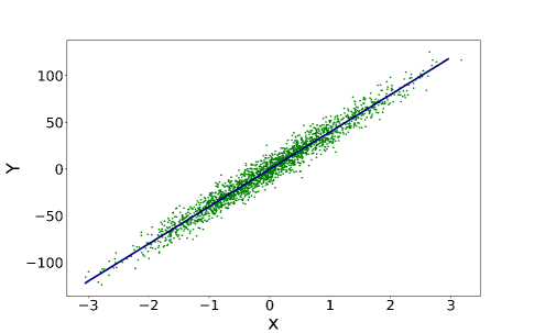
Figure 1: An application of linear regression to randomly generated data. The data was created using the make_regreession function from the libray sklearn.datasets.

Linear regression looks for a linear relationship between an independent variable, x or the input, and a dependent variable, y or the output. The algorithm fits a linear model to minimize the residual sum of squares difference between observed and predicted data, as shown in figure (1). In this method, it is possible to force the coefficients to be positive, which could be useful for some physical problems.

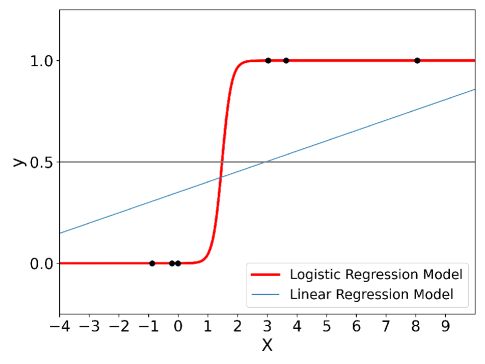
Figure 2: An example of logit function, superimposed with case of linear regression.

Logistic regression is a statistical method applied to cases where the input data needs to be labeled into different categories (Dalpiaz et al., 2021). It is a special case of linear regression where the output variable is a single value. Logistic regression uses probability theory to predict whether anything belongs to a group or not. This type of problem is known as a “binary classification problem” as one classifies an object as either belonging to a group or not. In this case, there are two possible results: “yes” and “no”. Usually, a positive result points to the presence of some identity separate from those of its members while a negative result points to the absence of it. Thus, one needs to predict the probability that identity is present. In practice, the binary responses variable is coded using 1 and 0 for “yes” and “no”, respectively.

To do so, we fit the function logit to the set of training data to map any real value to value in the interval between 0 and 1 based on a linear combination of dependent predictor variables as:

$$logit{P_{i}}=log\left(\frac{P_{i}}{1-P_{i}}\right)={\beta}_{0}+{\beta}_{1}x_{1,i}+{\beta}_{2}x_{2,i}+...+{\beta}_{k}x_{k,i},$$ (1)

where $P_{i}$ is the probability of the event i term, and the coefficients ${\beta}_{i}(i=1,2,...,k)$ are parameters of the model usually estimated through the maximum likelihood estimation (MLE) and $x_{i}(i=1,2,...,k)$ is a vector containing discrete or continuous values (Cramer, 2004; Gudivada et al., 2016). An example of logit function is shown in figure (2).

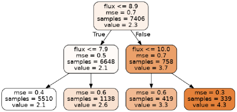
Figure 3: Decision tree regressor. 7406 objects from the Gaia Data Release 2 (Gaia Collaboration et al., 2018) are used to train a decision tree algorithm to found correlations between the relative flux uncertainties and the diameter measurements of the object (de Souza et al., 2021).

A Decision tree is a model that is described by a top-to-bottom tree-like graph. It can be used in both classification and regression. Decision tree algorithms make decisions in a tree-shaped form, as consecutive nodes. The lowest nodes in the tree are called leaves or terminal nodes. They are not associated with a condition, but instead, carry the label of a path within the tree. The number of decision nodes, or the maximum depth, “max$\_$depth”, is a free parameter of the model. An example of a tree diagram for a Decision tree is shown in figure (3), where we display the path to classify a sample of asteroids from the Gaia Data Release 2 (Gaia Collaboration et al., 2018), as used by (de Souza et al., 2021). In the first node of this regressor, all the objects with relative flux uncertainties $\leq 9$, in a logarithmic scale, will follow the arrow marked as True, and the rest will follow the False arrow. Other decisions will follow as marked.

Ensemble methods use several standalone algorithms to obtain a result. We can distinguish between:

1. Bootstrap aggregation (bagging): the training data is divided into several samples, called bootstrap samples, obtained by selecting a random sample with replacement of the training set. Each model is counted with the same weight.

2. Boosting: emphasizes the training cases where the previous models made fewer mistakes in the classification, and the autonomous models that had a better performance.

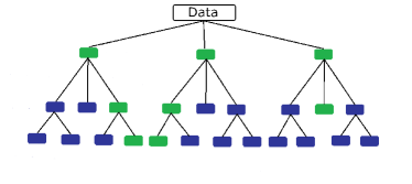
Figure 4: An example of the procedure used by Random Forest to reach decisions.

Examples of Bagging Classifiers are the Random Forest and the Extremely Randomized Trees. For Random Forest, a multitude of decision trees is created at training time. For classification tasks, the Random forest’s output is the class chosen by the majority of trees (Ho, 1995, 1998). The mean or average prediction of the individual trees is returned for regression tasks. Extremely Randomized Trees, or ExtraTree, follows a similar procedure, but the bagging process is performed without substitutions. An example of the procedure used by Random Forest to reach an outcome is shown in figure (4).

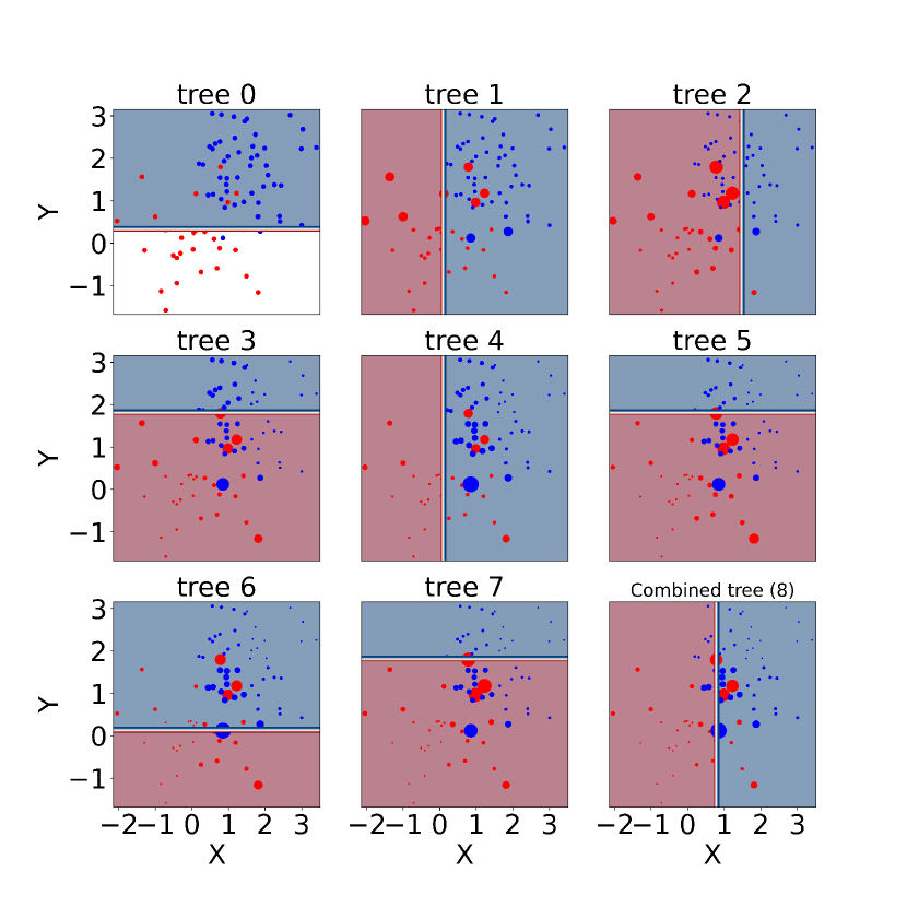
Figure 5: An illustration of the method by which Adaboost reaches decisions. The algorithm combines weak learners, assigns weights to incorrect values, and implements sequential tree growing considering past mistakes.

Examples of Boosting algorithms are Adaptive Boosting (AdaBoost), Gradient Boosting (Gboost), and eXtreme Gradient Boosting (XGBoost). In the AdaBoost method (Freund and Schapire, 1995), the reinforcement algorithms track the models that provided the least accurate forecast and give them lesser weights. The final result is achieved as a weighted average of the result of each autonomous model, as also shown in figure (5). GBoost differs from AdaBoost because it employs a gradient descent algorithm in the process of assigning weights to the standalone models’ outcome (Boehmke and Greenwell, 2019). The Gradient algorithm was regularized and optimized in XGBoost by Chen and Guestrin (2016).

Another example of ensemble tree-based methods are the Bayesian additive regression trees ($BART$) (Chipman et al., 2010; Hill et al., 2020). $BART$ is a model in which each tree is limited by a regularization before being a weak learner, and fitting and inference are carried out using an iterative Bayesian back-fitting algorithm that generates samples a posterior. While not a part of the standard Python scikit-learn package, $BART$ is available in Python at the GitHub repository “https://github.com/JakeColtman/bartpy”, last accessed on June 1st 2022.

Naive Bayes is a simple approach for creating classifiers, which are models that offer class labels to problem cases represented as vectors of feature values, with the class labels selected from a limited set. There is no single technique for training such classifiers; rather, there are several algorithms based on the same principle: all Naive Bayes classifiers assume that the value of one feature is independent of the value of any other feature, given the class variable. For example, a fruit is called an apple if it is red, round, and has a diameter of roughly 10 cm. A robust Naive Bayes classifier considers each of the color, roundness, and diameter features to contribute independently to the likelihood that this fruit is an apple (Piryonesi and El-Diraby, 2020), regardless of any possible correlations between them. The continuous values associated with each class are assumed to follow a normal distribution in the Gaussian Naive Bayes method.

Finally, Support-Vector Machines (SVM) have also been recently used for classification and regression problems (Cortes and Vapnik, 2009). Assume that some data points are assigned to one of two classes, and the purpose is to determine which class a new data point will be assigned to. A data point is seen as a $p$-dimensional vector (a list of $p$ numbers) in support-vector machines, and we want to know if we can separate such points with a $(p-1)$-dimensional hyperplane. Numerous hyperplanes might be used to categorize the data. The hyperplane that represents the greatest separation, or margin, between the two classes is a viable choice as the best hyperplane. The algorithm upon which SVMs are based automatically selects the best hyperplane.

2.2 Unsupervised learning

Unsupervised learning is a general term that incorporates a large set of statistical tools used to perform data exploration. Here we are going to review mostly algorithms used for clustering, which is the problem of arranging a set of items so that objects in the same group (called a cluster) are more comparable (in some sense) to those in other groups (clusters), and for anomaly detection, which is a step in data mining that identifies data points, events, or observations that deviate from a dataset most observed behavior. Concerning clustering, K-Nearest-Neighbors (KNN), k-means, and the Hierarchical Clustering Method (HCM) were the most used methods in recent literature, while recently published papers that worked with anomaly detection used Isolation forests. All the algorithms that we outline in this section are available in the Python library scikit-learn (Pedregosa et al., 2012).

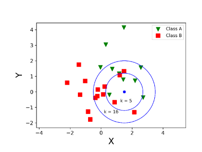
Figure 6: An example of bi-dimensional application of KNN for classification into two classes.

The basic idea behind KNN is to predict the status of a point based on its closest neighbors. If most of the closest neighbors belong to a class, the point is also classified as such. A free parameter of this algorithm is the number of neighbors used for the classification. Figure (6) shows a case where, if we use three as a number of neighbors, the central point will be classified as belonging to class B, while for a larger sample of 7 the point is classified as belonging to class A. KNN can be used for both supervised and unsupervised learning. Most recent applications used for problems of unsupervised learning, which is why we decided to list it in this section.

K-means, a centroid-based clustering technique, is one of the most extensively used clustering methods (MacQueen, 1967). The distance assignment between the objects in the sample is the first stage in K-means. The Euclidean metric is the default distance, however other metrics that are better relevant for the dataset at hand can be utilized. The algorithm then chooses $k$ random items from the dataset to act as the initial centroids, with $k$ being an external free parameter. The closest of the $k$ centroids is then allocated to each object in the dataset. The average position of the objects associated with the specified cluster is then used to construct new cluster centroids. These two procedures, re-assigning objects to clusters based on their distance from the centroid and recomputing cluster centroids, are performed until convergence is achieved. Convergence can be described in a variety of ways, such as when the vast majority of objects (90 percent or more) are no longer reassigned to various centroids, or when the cluster centroids converge to a single position. The cluster centroids and an association of the individual objects to the different clusters are the algorithm’s output.

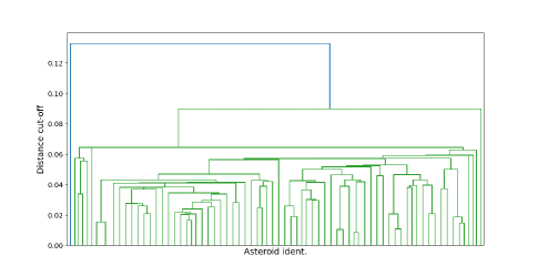
Figure 7: A dendrogram for classifying asteroid lightcurves using $HCM$ in domains of three non-periodic quantities. Adapted from figure (12) of Carruba and Aljbaae (2021).

HCM is the most commonly used method for identifying families of asteroids (Bendjoya and Zappalà, 2002). First, it checks for objects closer to a parent body than to a distance cut-off. If a new object is found, the new body is used as the parent body and the process is repeated until no new members are identified. Results of HCM are usually displayed in form of a dendrogram, as shown in figure (7), where HCM has been used to find groups in a domain of three non-periodic quantities of asteroid light curves. Each vertical line in the dendrogram represents a cluster, while each horizontal line is associated with the merging of groups. The vertical axis displays the distance cut-off.

Finally, concerning anomaly detection algorithms, Isolation forest is the first anomaly detection algorithm to use isolation to identify anomalies. It was first conceived and developed by Liu et al. (2008). Anomalies are described as those instances in the dataset that do not conform to the normal profile, according to the most common methodologies for anomaly detection. Isolation forest takes a different approach: instead of attempting to construct a model of normal examples, it separates anomalous points in the dataset explicitly. The key benefit of this approach is the ability to use sampling techniques in ways that profile-based methods cannot, resulting in a fast algorithm with low memory requirements.

In the next sub-section we are going to review $ML$ methods recently applied in the fields of time-series analysis.

2.3 $ML$ application in time-series analysis

Time-series analysis studies data points collected over a period of time. This form of study, on the other hand, is more than just gathering data over time. The ability to depict how variables change over time distinguishes time-series data from other types of data. In other words, time is an important variable since it reveals how the data changes through time as well as the final outcomes.

In this review paper, we are going to discuss two $ML$ methods that have been recently used for studies of asteroid dynamics, $ARIMA$ models and the use of auto-correlation functions $ACF$. Other methods, like the use of Exponential smoothing models ($ETS$) or the use of deep learning approaches based on artificial neural networks will not be treated in this section. Interested readers can find further details on these topics in Brownlee (2020). Numerical methods discussed in this section are available in the Python library statsmodels (Seabold and Perktold, 2010).

One exciting area where $ML$ has been recently applied is time-series analysis. Auto-regressive (AR), integrated (I), moving average (MA), or ARIMA models have been developed to predict stock prices behavior (Mills, 1999). Recent applications of $ARIMA$ models include Fraud detection in Credit Card transactions (Moschini et al., 2020), studies of variable stars light curves (Feigelson et al., 2018), and studies of coronal index solar cycles (Akhter et al., 2020), among others.

In an auto-regressive (AR) process current values depend on past ones through a relationship:

$$x_{t}=a_{1}x_{t-1}+a_{2}x_{t-2}+...+a_{p}x_{t-p}+{\epsilon}_{t},$$ (2)

where ${\epsilon}_{t}$ is a normally distributed error with constant variance and zero mean, $p$ is the process order (i.e., how many time lags are employed in the model), and $a_{i}(i=1,2,...,p)$ are the model coefficients for each lag up to order $p$. Current values in a moving average (MA) process are influenced by recent errors, or shocks, via the following relationship:

$$x_{t}={\epsilon}_{t}+b_{1}{\epsilon}_{t-1}+b_{2}{\epsilon}_{t-2}+...+b_{q}{\epsilon}_{t-q},$$ (3)

where ${\epsilon}_{t}$ is the error term for the t-th term, and the coefficients $b_{i}(i=1,2,...,q)$ quantify the response to the previous shocks up to order $q$. Adding the two equations produces an ARMA(p,q) model. The coefficients $a_{i}$ and $b_{i}$ are estimated using regression procedures, like the maximum likelihood estimation.

The ARMA model operates under several assumptions, that include the series being stationary, i.e., with constant mean and variance. A stationary series presents the same behavior at all times. Stationarity in a time series can be checked by performing tests such as the Dickey-Fuller, also known as Adfuller test (Dickey and Fuller, 1979). This test can be used by verifying the null hypothesis that a unit root is present in an AR model. If the probability $p_{AF}$ associated with the null hypothesis is less than 0.05, the series can be assumed to be stationary. A non-stationary series can be transformed into a stationary one by taking the difference of all elements with respect to their previous ones. If the new difference series is stationary, a modelization of this new series can then be carried out. If that is not the case, a new difference series can be computed from the order 1 difference series, and then checked for stationarity. The process can be then repeated until stationarity is achieved.

ARIMA models depend on three free parameters, $(p,d,q)$. These are the order $p$ of the autoregressive part of the model, the order $d$ of series differentiation by which stationarity is achieved, and the order $q$ of the moving average part. These coefficients can be determined using the Box-Jenkins approach (Box and Jenkins, 1976).

Other astronomical applications based on time series analysis were based on the autocorrelation function. Chaos in dynamical systems can be identified using an approach based on the autocorrelation function of time series, the ACF index (ACFI). The Pearson correlation coefficient (Pearson, 1895) measures how strong two time series are related. $R$ is near to 1, the maximum value, if the two variables depicted by the series are tightly connected. $R$ will be close to the minimal value of -1 if they are significantly anti-correlated, and $R\simeq 0$ if there is no correlation at all. A correlation coefficient can be defined in a variety of ways, but Pearson’s approach is the most frequent. If the i-th term of the series in $x$ and $y$ is defined as $x_{i}$ and $y_{i}$, then:

$$R=\frac{cov{(X,Y)}}{{\sigma}_{X}{\sigma}_{Y}},$$ (4)

where $cov{(X,Y)}$, which is the covariance of the two series, is defined as:

$$cov{(X,Y)}=\frac{1}{N^{2}}\sum_{i=1}^{N}\sum_{j=1}^{N}\frac{1}{2}(x_{i}-x_{j})(y_{i}-y_{j}).$$ (5)

$N$ is the number of terms in the two series, and ${\sigma}_{X}$ is the standard deviation of the $x_{i}$ series, defined as:

$${\sigma}_{X}=\sqrt{\frac{1}{N}\sum_{i=1}^{N}(x_{i}-{\mu}_{x})^{2}},$$ (6)

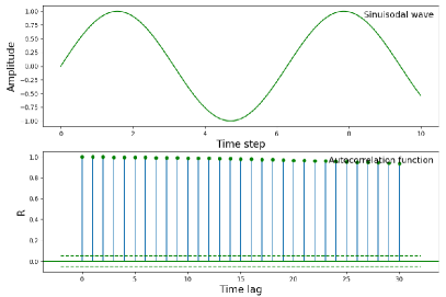
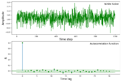
Figure 8: On the left, we have a plot of a sinusoidal wave’s time behavior (top panel) and its autocorrelation function (bottom panel). We have simulated white noise (top panel) and its $ACF$ on the right side (bottom panel). In the $ACF$ plots, the area between dashed horizontal lines represents the region where autocorrelation coefficients are less than 5% and represent negligible autocorrelation. Adapted from figure (1) of (Carruba et al., 2021a).

where ${\mu}_{x}=\frac{1}{N}\sum_{i=1}^{N}x_{i}$ is the average value of the series. For ${\sigma}_{Y}$, a similar expression exists. The correlation function of a time series with a lagged copy of the series is the autocorrelation coefficient of the series. Assume we have built a time series with a lag of one, $y_{i}=x_{i-1}$. Equation (4) will be used to calculate the autocorrelation coefficient for this $y_{i}$. For lags of 2 ($y_{i}=x_{i-2}$), 3 ($y_{i}=x_{i-3}$), and so on, analogous autocorrelation coefficients can be found. The spectrum of autocorrelation coefficients for various values of the time lag is the autocorrelation function ($ACF$) of $x_{i}$. The autocorrelation function is useful for determining the predictability of a series’ temporal behavior.

For a function that periodically repeats itself, all its auto-correlation coefficients are equal to 1 (see figure (8)). It is always possible to predict its future behavior. For white noise time series, such as random variables, all its auto-correlation coefficients are around 0. It is not possible to predict the series future behavior.

We can define a chaos indicator using the ACF, the auto- correlation function indicator (ACFI), as:

$$ACFI=\frac{1}{i_{fin}-i_{in}}\sum_{i=i_{in}}^{i=i_{fin}}n_{i}(\left|R\right|)>0.05),$$ (7)

where $n_{i}(\left|R\right|)>0.05)_{i}$ is the number of autocorrelation coefficients larger, in absolute value, than 5%, the null hypothesis for auto-correlation. ACFI is computed over the interval $i_{fin}-i_{init}$ to avoid including auto-correlation at short timescales.

2.4 Deep learning

Deep learning is part of a larger family of machine learning methods based on artificial neural networks. There are three types of learning for deep learning methods: supervised, semi-supervised, and unsupervised. Artificial neural networks (ANNs) were inspired by biological systems’ neuron networks. A typical ANN has numerous layers between the input and output layers, as shown in figure (9), which depicts a neural network with an input, a hidden layer, and an output layer. Neural networks come in a variety of shapes and sizes, but they all include the same basic components: neurons, weights, biases, and activation functions. These components function in a similar way to the human brain and may be trained in the same way as any other conventional ML method. While the terms Deep learning and artificial neural networks are often used interchangeably in some literature, there is a significant difference between the two. Neural networks use neurons to convey data in the form of input values and output values through connections, while deep learning is connected with feature transformation and extraction, which aims to build a relationship between stimuli and the corresponding neural responses. For the sake of simplicity, here we are going to use the term deep learning in a broader sense, which includes simple applications of neural networks. The reader is advised that this may not be a generally accepted practice.

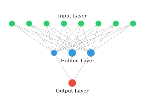
Figure 9: An example of a basic architecture of a neural network.

Three types of neural networks are among the most used in astronomy:

1. Multilayer Perceptron ($MLP$).

2. Long short-term memory ($LTSM$).

3. Convolutionary Neural Networks ($CNN$)

A $MLP$ is a type of feedforward $ANN$, and is typically composed by a network of multiple layers of perceptrons. A single perceptron is a function that can decide whether or not an input, represented by a vector of numbers, belongs to some specific class (Freund and Schapire, 1999). A feedforward $ANN$ is a network in which nodes do not form a cycle of connections, but only propagate forward. There are at least three levels of nodes in an $MLP$: an input layer, a hidden layer, and an output layer (see also figure (9)). Each node, except for the input nodes, is a neuron with a nonlinear activation function. Backpropagation is a supervised learning technique used by $MLP$ during training (Rosenblatt, 1963). $MLP$ were very popular in the 1980s for problems like speech and image recognition, but other methods like $CNN$ have been more commonly used for the latter applications more recently (Duev et al., 2019). The latest applications of $MLP$ are in the field of time series forecasting (see Brownlee (2020)).

$LSTM$ is a deep learning architecture based on an artificial recurrent neural network ($RNN$). Unlike normal feedforward neural networks, $LSTM$ has feedback connections, which allows them to handle not only individual data points (such as photos), but also complete data streams (such as speech or video). Applications of $LSTM$ in astronomy include time series forecasting (Brownlee, 2020) and time series anomaly detection (Malhotra et al., 2015).

$CNN$ are regularized versions of multilayer perceptrons. Multilayer perceptrons are typically completely connected networks, meaning that each neuron in one layer is linked to all neurons in the following layer. These networks’ ”complete connectedness” makes them vulnerable to data overfitting. Regularization, or preventing overfitting, can be accomplished in a variety of methods, including punishing parameters during training (such as weight loss) or reducing connectivity (skipped connections, dropout, etc.). To create patterns of increasing complexity, $CNN$s employ a different method of regularization: they take advantage of the hierarchical structure in data and use smaller and simpler patterns imprinted in their filters. $CNN$s have shown to be effective on difficult computer vision issues, reaching state-of-the-art results on tasks like picture classification while also serving as a component in hybrid models for completely new problems like object localization, image captioning, and more (Brownlee, 2020). Because of their effectiveness, they are the most commonly used $ANN$ architecture for image detection of Solar System small bodies (Duev et al., 2019, 2021).

Finally, more complex architecture involving combinations of $LSTM$ and $CNN$ are also possible and have been discussed in Brownlee (2020). Deep learning Python routines are available in the Tensorflow (Abadi et al., 2015) and Keras packages (Chollet and others, 2018). Because of their applications to image processing, Convolutional Neural Networks ($CNN$) can also very efficiently run on graphics processing unit (GPUs) (Strigl et al., 2010), and, more recently, have found applications in Tensor Processing Units (TPUs) (Yazdanbakhsh et al., 2021). Interested readers can find more information on the subject in the above references.

3 Applications to Solar System small bodies

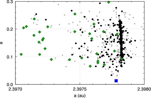
Figure 10: Asteroids in the resonances 4J-2S-1. Grey dots are resonant asteroids from a previous catalog. Black dots are newly identified resonant asteroids according to the $ML$ method, blue squares are resonant asteroids not identified by $ML$, and green diamonds display false positive identification by $ML$. Adapted from figure (1) by Smirnov and Markov (2017) and reproduced with permission from the author and MNRAS (©MNRAS).

Smirnov and Markov (2017) applied KNN, Decision tree, Gradient boosting, and Logistic regression to identify resonant three-body asteroids in the main belt. The results of identification by machine learning methods were accurate and take much less time than numerical integration (seconds versus days). The authors identified 404 new asteroids in the 4J-2S-1A three-body resonance using a machine-learning methodology (see figure (10)).

The subdivision of the observed objects of the Kuiper Belt (KBOs) into different dynamic classes is based on their orbits. Smullen and Volk (2020) used a GBoost model to automatically classify newly discovered objects into four classes.

Some families of asteroids may also be the result of spin-up-induced fission of a parent body in critical rotation (fission clusters, Pravec et al. (2010)). In at least four young groups of fission, more than 5% of its members belong to subfamilies. K-means can be used to automatically identify these groups (Carruba et al., 2020b).

Carruba et al. (2019) applied hierarchical clustering algorithms HCM for supervised learning to identify families of asteroids. This approach can find family members with scores above 89.5%. The authors identify 6 new families and 13 new clusters in regions where the method can be applied.

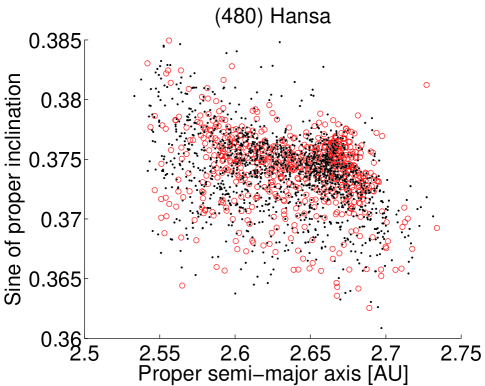
Figure 11: An $(a,\sin{(i)})$ projection of known members of the Hansa asteroid family. Asteroids predicted to be possible new members by ExtraTree are displayed as red circles.

Carruba et al. (2020a) used machine learning classification algorithms to identify new family members based on the orbital distribution in $(a,e,sin(i))$ of previously known family members. They compared the result of nine classification algorithms for autonomous and joint approaches. The Extremely Randomized Trees (ExtraTree) method had the highest precision, allowing to recover up to 97% of the family members identified with the standard HCM method. An application of this method to the Hansa asteroid family is shown in figure (11), where previously known family members are shown as black dots, and members predicted by the ExtraTree approach are red circles.

Selecting the ideal machine learning model and its hyperparameters can be a difficult task, especially when the domain of hyperparameters to be optimized is vast. Genetic algorithms (Chen et al., 2004) have this name because they mimic the process of genetic evolution. They have recently been used to select the ideal algorithm for predicting the asteroid population in the secular resonances $z_{1}$ and $z_{2}$, which are resonances involving the commensurabilities $g-g_{6}+s-s_{6}$ and $2(g-g_{6})+s-s_{6}$, where $g$ is the precession frequency of the longitude of pericenter, $s$ is the precession frequency of the longitude of nodes, and the suffix 6 identify Saturn, the sixth planet (Carruba et al., 2021a).

If we extend the field to general applications to asteroids, including observations, imaging, and taxonomy, three more works were produced in the last few years.

de Souza et al. (2021) used a logistic Bayesian additive regression tree model ($BART$) to find correlations between relative large flux uncertainties and systematic right ascension errors and large diameters in the Gaia database.

Taxonomic classification of NEA (Erasmus et al., 2017) and MBA (Erasmus et al., 2018) based on VRI spectrophotometry data was recently obtained with algorithms using KNN, SVM, and a Gaussian Naive Bayes method developed by Mommert et al. (2016).

Chen et al. (2018) used an algorithm developed by Lin et al. (2018) and based on Random forest and Isolation forest for the supervised and unsupervised learning to detect moving objects, including asteroids, from images obtained from the Hyper Suprime-Cam Subaru Strategic Program (HSC-SSP).

Asteroid’ brightness is not generally constant, but presents time variations that depend on the asteroid shape, albedo, rotation period, and other factors. ARIMA models can fit the light curve shapes with an error of less than 1%, even for very complex shapes. Based on the order of the best-fitting model $(p,d,q)$, a new classification scheme for asteroid light curves can be introduced (Carruba and Aljbaae, 2021).

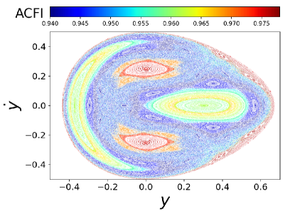
Figure 12: A 2D Poincaré Surface of Section ($PSS$) with for the Hénon-Heiles system with $H=0.125$ and $ACFI$ values. Adapted from figure (4) of (Carruba et al., 2021a).

$ACFI$ can be applied to well-known systems, like the Hénon-Heiles Hamiltonian (see figure (12)). For Solar System small bodies, it can be used to separate the effects of resonance overlapping from close encounters with massive bodies (Carruba et al., 2021a).

Neural networks can be used to predict the orbital stability of asteroids in the main belt. Liu et al. (2021) used ANN to fit data obtained from the integration of 151,000 orbital initial conditions. A temporal stability map in the $(a,e)$ plane was obtained as a result.

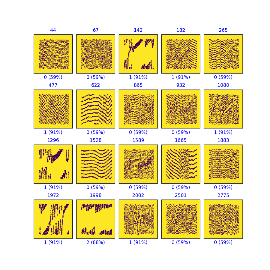
Figure 13: A set of 20 images of asteroids in or near resonant states of the 1:2 MMR (mean-motion resonance) with Mars. The x-axes display the predicted classification (0 for circulating orbits, 1 for switching and 2 for librating ones) and their probabilities of belonging to a given class. The titles of each figure panel are the asteroid identifications.

Neural networks can also be used to automatically recognize images from time series. This allows one to automatically determine whether an asteroid is in resonance or not, as performed by (Carruba et al., 2021b) for asteroids near the $M1:2$ mean-motion resonance. Figure (13) displays a set of 20 images of resonant arguments for 20 such asteroids. The first panel displays the time behavior of an argument for an asteroid in a circulating orbit, the seventeenth one that of an asteroid in a librating state, and the third panel shows the case of an asteroid alternating phases of libration and circulation. Similar sets of images can be used to train artificial neural networks so that the process of identifying the resonant state is performed automatically.

Aljbaae et al. (2021) applied a Time-Series prediction with Neural Networks in Python with Keras to identify non-chaotic behavior of spacecraft close to the asteroid (99942) Apophis during its exceptionally close approach with Earth on 2029 April 13, at about 38 000 km from the Earth’s center. The authors classify orbits based on a relationship between the difficulty in the prediction and the stability. This method can isolate the most regular orbits that could be stable in the system. A good correlation was found between the Time-Series prediction approach and MEGNO (Cincotta and Simó, 2000) or the Perturbation Map of type II (PMap) (Sanchez and Prado, 2017, 2019). Pugliatti and Topputo (2020) adopted a CNN approach for the small-body shape recognition task. The authors obtained very good performances of their model, with a precision of 98.52%. Meaningful results are also presented with varying illumination conditions.

Finally, Li et al. (2022) recently used $ANN$ to predict the trajectories of the 2:3 Neptune resonators over periods of $\simeq$ 20000 yrs. The outcome of the model can predict the resonant angle with an accuracy as small as of a few degrees. This approach, faster that standard numerical methods, can help in identifying populations of KBOs to be discovered in future surveys.

If we extend the field to include the detection and imaging of small bodies, a series of related papers have been published in the last years. Duev et al. (2019) created DeepStreaks in 2019, a convolutional neural network, deep-learning system designed to efficiently identify streaking fast-moving near-Earth objects identified in the Zwicky Transient Facility (ZTF), a wide-field, time-domain survey. The method cut human involvement in the streak detection process by orders of magnitude, from several hours to less than 10 minutes every day.

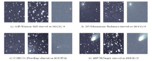
Figure 14: A set of images used by Tails for the purpose of training $ANN$s to recognize comets image data. Image adapted from the figure (1) of Duev et al. (2021) and reproduced with permission of the American Astronomical Society (©AAS).

Duev et al. (2021) also developed Tails, an open-source deep-learning framework for the identification and localization of comets in the image data of the Zwicky Transient Facility (ZTF). Tails employs a custom EfficientDet-based architecture and is capable of finding comets in single images in near-real-time (see figure (14) for an example of images used to train the ANN. Information on the ANN architecture is available in figure (1) of Duev et al. (2021)). This includes the first AI-assisted discovery of a comet (C/2020 T2) and the recovery of a comet (P/2016 J3 = P/2021 A3).

Neural networks can also be used to automatically classify asteroids into their taxonomic spectral classes. Penttilä et al. (2021) used feed-forward neural networks to predict asteroid taxonomies with the Bus-DeMeo classification using datasets simulating GAIA observations, and, more recently, simulating Legacy Survey of Space and Time (LSST) observations (Penttilä et al., 2022). Results show that neural networks can identify taxonomic classes of asteroids in a robust manner.

4 From classification to insight: assessing the impact of machine learning applications to asteroid dynamics

Fluke and Jacobs (2020) utilized seven categories to assess recently published literature, where the last two are those with a higher scientific outcome.

1. Classification: objects or features are assigned to one of several categories or labels. The machine learning algorithm learns the properties that link an instance to a category based on a training set (labeled or unlabeled). When the algorithm is applied to a new instance, it assigns the most likely category label.

2. Regression: The assignment of a numerical value (or values) based on the characteristics that the machine learning algorithm has learned or otherwise predicted. A training set, similar to classification, can be utilized, or the features might be deduced from the data set.

3. Clustering: these techniques assess if an object or feature is a part of (or a member of) anything. This could be a physical structure or association, like an asteroid family, or a region within an N-dimensional parameter space.

4. Forecasting: The machine learning algorithm’s goal is to learn from prior occurrences and anticipate or forecast the occurrence of a similar event. The forecast has an inherent time dependence.

5. Generation and Reconstruction: Missing information is generated and reconstructed, with the expectation that it will be consistent with the underlying truth. The absence of information could be caused by noise, processing artifacts, or other astronomical events, all of which conspire to obfuscate the required signal.

6. Discovery: New celestial objects, features, or relationships are discovered as a result of using a machine learning or artificial intelligence technology.

7. Insight: New scientific knowledge is demonstrated as a result of applying machine learning, which goes beyond the finding of astronomical objects. This includes situations where information about the suitability of using machine learning, data set selection, hyperparameters, and comparisons to human-based classification is gathered.

Classification, regression, and clustering methods are frequently compared to a comparable human-centered approach, but with the need to “scale-up” either the size of the dataset to be studied or the time it takes to complete the work. The results of classification and regression can be the culmination of an investigation or the input to a forecasting, generating, finding, or insight process.

These seven categories, which constitute a loose hierarchy of sophistication, provide an assessment of the maturity of the use of machine learning and artificial intelligence within a subfield of astronomy. Using a machine learning technique to conduct a classification, regression, or clustering problem is a frequent starting point. Machine learning can be used to estimate expected future outcomes, like future solar flares (Florios et al., 2018), or produce discoveries, like the identification of new candidates of rare objects (Zhang et al., 2018), once it has been established as being comparable to, or exceeding, a more traditional approach.

How can papers published in the field of asteroid dynamics and Solar System small bodies be classified in terms of these categories? We can divide the field into five main types of subfields:

1. Resonant and chaotic dynamics: in this subfield we consider papers that deal with the identification and classification of asteroidal populations in mean-motion and secular resonances, or deal with the effects of chaotic motions either caused by resonant dynamics or stochastic effects, like close encounters with massive bodies.

2. Asteroid families’ identification: articles that deal with identifying new members of known or newly identified asteroid groups, which could either be dynamical families or groups produced by rotational fission.

3. $ML$ applications to time series analysis: articles that focus on the prediction and classification of a time series, which could be a time series of orbital elements, an asteroid light curve, or other applications.

4. Image recognition: these are papers that mostly use Artificial Neural Networks (ANN) to recognize patterns or images. Applications include asteroid or comets images, asteroid spectra, and asteroid resonant arguments, among others.

5. Asteroid taxonomy and physical properties: papers that focus on obtaining taxonomical information from spectral or spectrophotometric data, or physical properties like masses, shapes, and densities, using $ML$.

These categories are not mutually exclusive. For instance, papers that deal with resonant dynamics can use ANN to recognize images of resonant arguments (Carruba et al., 2021b). Articles that focus on chaos may use time series analysis techniques to identify regular and chaotic orbits (Carruba et al., 2021a). Once the number of papers in the field increases, other divisions into subfields may appear to be more useful for classifying research done in this area. For the time being, however, we will use this scheme to organize current papers in the field.

Table (1) displays our analysis of 12 papers in the field of machine learning applied to asteroid dynamics, and 21 in the broader area of Solar System small bodies. For each of the sub-areas that we introduced in this section, we classify if a paper covers one or more of the seven categories of scientific outcomes introduced by (Fluke and Jacobs, 2020). Results are also summarized for the whole subareas of asteroid dynamics and small bodies in figure (15). A more detailed classification, article by article, is also presented in table (2) in appendix (1).

Table 1: A qualitative summary of the categories of $ML$ algorithms and the most common subareas of research for asteroid dynamics (first four rows) and for the extended area of applications to small bodies (second set of five rows).

Nature/type	Classification	Regression	Clustering	Forecasting	Generation	Discovery	Insight
Res. & Chaotic Dyn	6	2	1	7	3	2	0
Ast. Fam. Id.	1	0	2	3	1	2	0
Time series An.	3	1	1	3	2	1	0
Image recognition	1	0	0	1	1	0	0
Res. & Chaotic Dyn	6	3	1	7	3	3	0
Ast. Fam. Id.	1	0	2	3	1	2	0
Time series An.	3	2	1	4	4	2	0
Image recognition	1	1	0	4	4	4	2
Ast. Tax. Phys	4	1	0	4	1	1	0

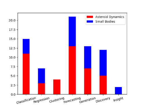
Figure 15: A bar plot summarizing the data from table (1) for the categories of $ML$ algorithms applied to asteroid dynamics (blue bars) and small bodies (red bars).

What can be learned from this analysis? Fluke and Jacobs (2020) used a hierarchy of three categories to evaluate the maturity of $ML$ within a subfield of astronomy: emerging, progressing, and established.

The emerging stage is used for astronomy and astrophysics subfields that are beginning to study the use of machine learning and artificial intelligence, generally by attacking easier to solve problems. This could be a challenge that necessitates a classification or regression strategy, or a comparison of machine learning and another, well-known method. For emerging communities, the $ML$ methodologies best suited to a given problem may have not yet been encountered, or the community is tiny.

In a progressing stage, a greater range of approaches are utilized, or a single technique is used several times, or there is an immediate jump to the forecasting, discovery, or insight phases in fields regarded as progressing in their usage of ML.

Finally, a subfield reached an established stage if the application of machine learning has become essential in established subfields, there is a considerable body of research, and the focus is mostly on predicting, discoveries, or insight. It is no longer necessary to assess the applicability of machine learning because its application has become of wide use.

Fluke and Jacobs (2020) classified the study of Small bodies objects as having reached a progressing stage. Based on our analysis, we agree on this result: there is a wider community already studying Small bodies, which has produced works that produced scientific outcomes reaching the categories of discovery and insight, like the articles from Duev et al. (2019) and Duev et al. (2021), with the first $ML$-assisted discovery of a comet (C/2020 T2). More advanced techniques, like the use of neural networks for image recognition, are becoming more and more common in the area, almost reaching the status of an established method, associated with the (Fluke and Jacobs, 2020) progressing stage.

This is less true if we consider the subfield of asteroid dynamics. The community working in the area is less established, with six groups with published papers so far, fewer papers produced scientific outcomes that can be categorized as belonging to generation or discovery, and none reached the stage of insight. Overall, we believe that $ML$ applied to asteroid dynamics may be classified as still being in the emerging phase, but already approaching a progressing phase.

5 Future trends

Having reviewed recent literature in the field, it is now time to attempt to look for possible future trends in the area. In performing such a task one always runs the risk of painting a biased portrait, influenced by personal experiences and expectations. Yet, we think that this could be a useful thought experiment, and could at least form the base for a more educated discussion on the subject.

Most recent efforts have focused on the use of ANNs, either for classification of images of asteroid resonant arguments (Carruba et al., 2021b), for the detection of images of Solar System small bodies (Duev et al., 2019, 2021), or for classifying asteroids into their taxonomic spectral classes Penttilä et al. (2021, 2022). The use of more and more complex architecture of ANNs, as described in section (2.4), could significantly improve the speed and efficiency of the models currently used by the scientific community. It is reasonable to expect that some of the next scientific advancements may occur in this area.

An engine for progress in the field of $ML$ has been in the recent past Kaggle competitions (see also https://www.
kaggle.com/competitions, last accessed on June 1st 2022). Kaggle competitions are machine learning tasks made by Kaggle or other companies, like Google or WHO. Competitions range in types of problems and complexity, but they are generally open to novices. They usually award a monetary prize for the best problem solution. A recent example of a Kaggle-like competition in the field of asteroid dynamics has been a challenge hosted in Kelvins about the prediction of the effects of an impact while deflecting asteroids in the context of the HERA mission
(https://kelvins.esa.int/planetary-defence/, last accessed on August 5th, 2021). A dataset is provided to explore a way to do this task in a purely $ML$-driven way.

Another way in which the field could advance is by using algorithms that have found applications in other fields, but are not yet of common use among the small bodies community. Examples of these are density-based clustering algorithms, like DBSCAN and GDBSCAN, which can cluster point objects, as well as spatially extended objects according to both, their spatial and their non-spatial attributes (Sander et al., 1998).

Concerning deep learning algorithms, a very promising method is the Transformer architecture (Vaswani et al., 2017). Complex recurrent or convolutional neural networks with an encoder and a decoder are the most common sequence transduction models. The finest models additionally use an attention mechanism to connect the encoder and decoder. The Transformer is a new simple network architecture model purely based on attention processes, with no recurrence or convolutions. Experiments on two machine translation tasks reveal that these models are superior in quality, parallelizable, and take much less time to train.

Another area where applications of $ML$ are most likely to be of great importance is the analysis of data produced by next-generation astronomical surveys. We already saw that large databases produced by space missions like GAIA will need $ML$ methods to fully take advantage of the information available in the data (Penttilä et al., 2021). Ongoing observational robotic surveys, like those produced by the Zwicky Transient Facility ($ZTF$) (Dekany et al., 2020) have already produced modeling efforts in the $ML$ area, with the already discussed papers on the DeepStreaks (Duev et al., 2019) and Tails (Duev et al., 2021) software packages for the identification of fast-moving near-Earth objects and comets. $ZTF$ is a large optical survey in multiple filters producing hundreds of thousands of transient alerts per night. $ML$ is already commonly used for the analysis of such data, and plans to expand its implementations are already underway (Mahabal et al., 2019).

Data produced by $ZTF$ is, however, estimated to be just $\simeq$ 10% of what is expected from the Vera C. Rubin Observatory. This 8.4-meter three-mirror design telescope, currently under construction in Chile, is expected to start operations in October 2023. Jones et al. (2015) estimated that the catalogs generated by the Vera C. Rubin Observatory will increase the known number of small bodies in the Solar System by a factor of 10-100 times, among all populations, with $\simeq$ 1 million new asteroid discoveries predicted in just the first year of operations. The need to handle such a massive amount of data has already caused the development of new methods, like the use of Lomb-Scargle algorithm on Graphics Processing Units (Gowanlock et al., 2021). More $ML$-oriented software development is expected in the next years.

6 Conclusions

In this work, we reviewed 21 papers with applications of $ML$ to Solar System bodies, 12 of which had a focus on $ML$ applied to asteroid dynamics. A brief outline of the methods used in the reviewed references has been first provided, with references to the theoretical papers most relevant to each approach, and links to some of the most commonly used software packages for each method. Current references were then classified in terms of metrics recently used by Fluke and Jacobs (2020) to assess the impact of applications of $ML$ algorithms in other astronomical subfields.

$ML$ applications to Solar System bodies, which include imaging and spectophotometry of small bodies have already reached the progressing stage, with established research communities and methodologies, as well as papers describing how the use of $ML$ led to the discovery of new celestial objects, or features, or to new insights in the field. $ML$ applied to asteroid dynamics has seen many recent developments, especially in the Space missions to asteroids area. However, since fewer papers producing discoveries or insights are still produced, we believe that this area may be still considered as an emerging field, moving on to the progressing phase.

As discussed in section (5), the most recent efforts have focus on the use of ANNs, either for classification of images of asteroid resonant arguments, for the detection of images of Solar System small bodies, or for classifying asteroids into their taxonomic spectral classes Developments on the line of what was discussed in section (2.4), could in the next year significantly improve the speed and efficiency of methods currently used by the scientific community.

Finally, the development of new, more advanced, $ML$ algorithms, and the need to develop new methods able to handle the massive amount of data expected to be produced by robotic astronomical surveys, like the Zwicky Transient Facility ($ZTF$) and the Vera C. Rubin Observatory have already been a powerful motivation to develop new $ML$ methods for data analysis, as discussed in section (5). It is fair to expect many new exciting developments and discoveries in the field in the next few years.

7 Appendix (1): data on current applications of $ML$ in asteroid dynamics

Table 2: Reference data used to classify the status of application of machine learning to recent literature. The first column shows the article number, which refers to the order of citation in this work. The second column yields the reference to the cited work. The third column displays the types of machine learning applications, which could be either an application of supervised (SL) or unsupervised (UL) learning, time-series analysis (TSA), or deep learning (DL). The fourth column show if the article is in the field of asteroid dynamics (AD) or small bodies in the Solar System (SB). The fifth column shows the article field, which can be resonant and chaotic dynamics (RD), asteroid families’identification (AFI), time-series analysis (TSA), Image recognition (IR), asteroid taxonomy and physical properties (ATP), or space missions to asteroids (ASM). Finally, the sixth column shows the Fluke and Jacobs (2020) categories by which the scientific outcomes of the paper were classified in this work: Classification (C), Regression (R), Clustering (CL), Forecasting (F), Generation and Reconstruction (G), Discovery (D), and Insight (I). Multiple categories may apply to a single work.

Article	Reference	ML	Article	Subject	Category
number		application	Field	Subfield
1	Smirnov and Markov (2017)	SL	AD	RD	C,R,F
2	Smullen and Volk (2020)	SL	AD	AFI	R,CLF
3	Carruba et al. (2020b)	UL	AD	AFI	CL,F
4	Carruba et al. (2019)	UL	AD	AFI	CL,F
5	Carruba et al. (2020a)	SL	AD	AFI	C,F,D
6	Carruba et al. (2021a)	SL	AD	RD,AFI	R,F,G,D
7	de Souza et al. (2021)	SL	SL	ATP	C,F
8	Erasmus et al. (2017)	SL	SL	ATP	C,F
9	Erasmus et al. (2018)	SL	SL	ATP	C,F
10	Chen et al. (2018)	UL	SL	IR	R,D,I
11	Carruba and Aljbaae (2021)	TSA	AD	TSA	C,R,CL,F,G
12	Carruba et al. (2021a)	TSA	AD	RD,TSA	C,F,D
13	Liu et al. (2021)	DL	AD	RD	C,F,G
14	Carruba et al. (2021b)	DL	AD	RD,IR	C,F,G
15	Aljbaae et al. (2021)	DL	AD	RD,TSA	C,F,G
16	Duev et al. (2019)	DL	SL	IR	F,D,G
17	Duev et al. (2021)	DL	SL	IR	F,D,G,I
18	Penttilä et al. (2021)	DL	SL	ATP	C,F,G
19	Penttilä et al. (2022)	DL	SL	ATP	C,F,G
20	Pugliatti and Topputo (2020)	DL	AD	ATP	C,G
21	Li et al. (2022)	DL	SL	RD, TSA	R,F,G,D

In this section we report the data used to classify current literature according to Fluke and Jacobs (2020) category scheme, as discussed in section (4). Our data is shown in table (2).

Conflict of interest

The authors declare that they have no conflict of interest.

8 Author contributions

All authors contributed to the study conception and design. Material preparation, and data collection were performed by Valerio Carruba, Safwan Aljbaae and Rita Cassia Domingos. The first draft of the manuscript was written by Valerio Carruba and all authors commented on previous versions of the manuscript. All authors read and approved the final manuscript.

References

- Abadi et al. (2015) Abadi M, Agarwal A, Barham P, Brevdo E, Chen Z, Citro C, Corrado GS, Davis A, Dean J, Devin M, Ghemawat S, Goodfellow I, Harp A, Irving G, Isard M, Jia Y, Jozefowicz R, Kaiser L, Kudlur M, Levenberg J, Mané D, Monga R, Moore S, Murray D, Olah C, Schuster M, Shlens J, Steiner B, Sutskever I, Talwar K, Tucker P, Vanhoucke V, Vasudevan V, Viégas F, Vinyals O, Warden P, Wattenberg M, Wicke M, Yu Y, Zheng X (2015) TensorFlow: Large-scale machine learning on heterogeneous systems. URL https://www.tensorflow.org/, software available from tensorflow.org
- Akhter et al. (2020) Akhter MF, Hassan D, Abbas S (2020) Predictive ARIMA Model for coronal index solar cyclic data. Astronomy and Computing 32:100403, DOI 10.1016/j.ascom.2020.100403
- Aljbaae et al. (2021) Aljbaae S, Souchay J, Carruba V, Sanchez DM, Prado AFBA (2021) Influence of Apophis’ spin axis variations on a spacecraft during the 2029 close approach with Earth. Accepted by the Romanian Astronomical Journal arXiv:2105.14001, 2105.14001
- Ball and Brunner (2010) Ball NM, Brunner RJ (2010) Data Mining and Machine Learning in Astronomy. International Journal of Modern Physics D 19(7):1049–1106, DOI 10.1142/S0218271810017160, 0906.2173
- Baron (2019) Baron D (2019) Machine Learning in Astronomy: a practical overview. arXiv e-prints arXiv:1904.07248, 1904.07248
- Bendjoya and Zappalà (2002) Bendjoya P, Zappalà V (2002) Asteroid Family Identification, Arizona Univ. Press, pp 613–618
- Bezanson et al. (2017) Bezanson J, Edelman A, Karpinski S, Shah VB (2017) Julia: A fresh approach to numerical computing. SIAM review 59(1):65–98, URL https://doi.org/10.1137/141000671
- Boehmke and Greenwell (2019) Boehmke B, Greenwell B (2019) Gradient Boosting”. Hands-On Machine Learning with R. Chapman & Hall, London
- Box and Jenkins (1976) Box, Jenkins (eds) (1976) Time series analysis. Forecasting and control, San Francisco : Holden-Day
- Brownlee (2020) Brownlee J (2020) Deep Learning for Time Series Forecasting. Ed. Machine Learning Mastery, San Juan, PR, USA
- Carruba and Aljbaae (2021) Carruba V, Aljbaae S (2021) Predicting asteroid lightcurves using ARIMA models. In: European Planetary Science Congress, pp EPSC2021–36, DOI 10.5194/epsc2021-36
- Carruba et al. (2019) Carruba V, Aljbaae S, Lucchini A (2019) Machine-learning identification of asteroid groups. MNRAS488(1):1377–1386, DOI 10.1093/mnras/stz1795
- Carruba et al. (2020a) Carruba V, Aljbaae S, Domingos RC, Lucchini A, Furlaneto P (2020a) Machine learning classification of new asteroid families members. MNRAS496(1):540–549, DOI 10.1093/mnras/staa1463
- Carruba et al. (2020b) Carruba V, Spoto F, Barletta W, Aljbaae S, Fazenda ÁL, Martins B (2020b) The population of rotational fission clusters inside asteroid collisional families. Nature Astronomy 4:83–88, DOI 10.1038/s41550-019-0887-8
- Carruba et al. (2021a) Carruba V, Aljbaae S, Domingos RC (2021a) Identification of asteroid groups in the z1 and z2 nonlinear secular resonances through genetic algorithms. Celestial Mechanics and Dynamical Astronomy 133(6):24, DOI 10.1007/s10569-021-10021-z
- Carruba et al. (2021b) Carruba V, Aljbaae S, Domingos RC, Barletta W (2021b) Artificial neural network classification of asteroids in the M1:2 mean-motion resonance with Mars. MNRAS504(1):692–700, DOI 10.1093/mnras/stab914, 2103.15586
- Chen et al. (2004) Chen PW, Wang JY, Lee H (2004) Model selection of svms using ga approach. 2004 IEEE International Joint Conference on Neural Networks (IEEE Cat No04CH37541) 3:2035–2040 vol.3
- Chen and Guestrin (2016) Chen T, Guestrin C (2016) Xgboost. Proceedings of the 22nd ACM SIGKDD International Conference on Knowledge Discovery and Data Mining DOI 10.1145/2939672.2939785, URL http://dx.doi.org/10.1145/2939672.2939785
- Chen et al. (2018) Chen YT, Lin HW, Alexandersen M, Lehner MJ, Wang SY, Wang JH, Yoshida F, Komiyama Y, Miyazaki S (2018) Searching for moving objects in HSC-SSP: Pipeline and preliminary results. Publications of the Astronomical Society of Japan 70:S38, DOI 10.1093/pasj/psx145, %****␣ML_CMDA_14.bbl␣Line␣125␣****1705.01722
- Chipman et al. (2010) Chipman HA, George EI, McCulloch RE (2010) Bart: Bayesian additive regression trees. The Annals of Applied Statistics 4(1), DOI 10.1214/09-aoas285, URL http://dx.doi.org/10.1214/09-AOAS285
- Chollet and others (2018) Chollet F, others (2018) Keras: The Python Deep Learning library
- Cincotta and Simó (2000) Cincotta PM, Simó C (2000) Simple tools to study global dynamics in non-axisymmetric galactic potentials - I. Astronomy & Astrophysics, Supplement 147:205–228, DOI 10.1051/aas:2000108
- Cortes and Vapnik (2009) Cortes C, Vapnik V (2009) Support-vector networks. Chem Biol Drug Des 297:273–297, DOI 10.1007/%2FBF00994018
- Cramer (2004) Cramer J (2004) The early origins of the logit model. Studies in History and Philosophy of Science Part C: Studies in History and Philosophy of Biological and Biomedical Sciences 35(4):613–626, DOI https://doi.org/10.1016/j.shpsc.2004.09.003, URL https://www.sciencedirect.com/science/article/pii/S1369848604000676
- Dalpiaz et al. (2021) Dalpiaz et al (2021) Applied Statistics with R, STAT 420. University of Illinois at Urbana-Champaign, https://daviddalpiaz.github.io/appliedstats/
- de Souza et al. (2021) de Souza RS, Krone-Martins A, Carruba V, de Cassia Domingos R, Ishida EEO, Alijbaae S, Huaman Espinoza M, Barletta W (2021) Probabilistic Modeling of Asteroid Diameters from Gaia DR2 Errors. Research Notes of the American Astronomical Society 5(8):199, DOI 10.3847/2515-5172/ac205e, 2108.11814
- Dekany et al. (2020) Dekany R, Smith RM, Riddle R, Feeney M, Porter M, Hale D, Zolkower J, Belicki J, Kaye S, Henning J, Walters R, Cromer J, Delacroix A, Rodriguez H, Reiley DJ, Mao P, Hover D, Murphy P, Burruss R, Baker J, Kowalski M, Reif K, Mueller P, Bellm E, Graham M, Kulkarni SR (2020) The Zwicky Transient Facility: Observing System. Publications of the Astronomical Society of the Pacific 132(1009):038001, DOI 10.1088/1538-3873/ab4ca2, 2008.04923
- Dickey and Fuller (1979) Dickey DA, Fuller WA (1979) Distribution of the estimators for autoregressive time series with a unit root. Journal of the American Statistical Association 74(366a):427–431, DOI 10.1080/01621459.1979.10482531, URL https://doi.org/10.1080/01621459.1979.10482531, https://doi.org/10.1080/01621459.1979.10482531
- Duev et al. (2019) Duev DA, Mahabal A, Ye Q, Tirumala K, Belicki J, Dekany R, Frederick S, Graham MJ, Laher RR, Masci FJ, Prince TA, Riddle R, Rosnet P, Soumagnac MT (2019) DeepStreaks: identifying fast-moving objects in the Zwicky Transient Facility data with deep learning. MNRAS486(3):4158–4165, DOI 10.1093/mnras/stz1096, 1904.05920
- Duev et al. (2021) Duev DA, Bolin BT, Graham MJ, Kelley MSP, Mahabal A, Bellm EC, Coughlin MW, Dekany R, Helou G, Kulkarni SR, Masci FJ, Prince TA, Riddle R, Soumagnac MT, van der Walt SJ (2021) Tails: Chasing Comets with the Zwicky Transient Facility and Deep Learning. AJ161(5):218, DOI 10.3847/1538-3881/abea7b, 2102.13352
- Erasmus et al. (2017) Erasmus N, Mommert M, Trilling DE, Sickafoose AA, van Gend C, Hora JL (2017) Characterization of Near-Earth Asteroids Using KMTNET-SAAO. AJ154(4):162, DOI 10.3847/1538-3881/aa88be, 1709.03305
- Erasmus et al. (2018) Erasmus N, McNeill A, Mommert M, Trilling DE, Sickafoose AA, van Gend C (2018) Taxonomy and Light-curve Data of 1000 Serendipitously Observed Main-belt Asteroids. The Astrophysical Journal Supplement Series 237(1):19, DOI 10.3847/1538-4365/aac38f, 1805.04478
- Feigelson et al. (2018) Feigelson ED, Babu GJ, Caceres GA (2018) Autoregressive Times Series Methods for Time Domain Astronomy. Frontiers in Physics 6:80, DOI 10.3389/fphy.2018.00080, 1901.08003
- Florios et al. (2018) Florios K, Kontogiannis I, Park SH, Guerra JA, Benvenuto F, Bloomfield DS, Georgoulis MK (2018) Forecasting Solar Flares Using Magnetogram-based Predictors and Machine Learning. Solar Physics 293(2):28, DOI 10.1007/s11207-018-1250-4, 1801.05744
- Fluke and Jacobs (2020) Fluke CJ, Jacobs C (2020) Surveying the reach and maturity of machine learning and artificial intelligence in astronomy. WIREs Data Mining and Knowledge Discovery 10(2):e1349, DOI 10.1002/widm.1349, 1912.02934
- Freund and Schapire (1999) Freund Y, Schapire R (1999) Large margin classification using the perceptron algorithm. Machine Learning 37, DOI 10.1023/A:1007662407062
- Freund and Schapire (1995) Freund Y, Schapire RE (1995) A decision-theoretic generalization of on-line learning and an application to boosting
- Gaia Collaboration et al. (2018) Gaia Collaboration, Spoto F, Tanga P, et al (2018) Gaia Data Release 2. Observations of solar system objects. A&A616:A13, DOI 10.1051/0004-6361/201832900, 1804.09379
- Gowanlock et al. (2021) Gowanlock MG, Kramer DA, Trilling DE, Butler NR, Donnelly B (2021) Fast period searches using the lomb-scargle algorithm on graphics processing units for large datasets and real-time applications. Astron Comput 36:100472
- Gudivada et al. (2016) Gudivada V, Irfan M, Fathi E, Rao D (2016) Chapter 5 - cognitive analytics: Going beyond big data analytics and machine learning. In: Gudivada VN, Raghavan VV, Govindaraju V, Rao C (eds) Cognitive Computing: Theory and Applications, Handbook of Statistics, vol 35, Elsevier, pp 169–205, DOI https://doi.org/10.1016/bs.host.2016.07.010, URL https://www.sciencedirect.com/science/article/pii/S0169716116300517
- Hill et al. (2020) Hill J, Linero A, Murray J (2020) Bayesian additive regression trees: A review and look forward. Annual Review of Statistics and Its Application 7(1):251–278, DOI 10.1146/annurev-statistics-031219-041110, URL https://doi.org/10.1146/annurev-statistics-031219-041110, https://doi.org/10.1146/annurev-statistics-031219-041110
- Ho (1995) Ho TK (1995) Random decision forests. In: Proceedings of the Third International Conference on Document Analysis and Recognition (Volume 1) - Volume 1, IEEE Computer Society, M, ICDAR ’95, pp 278–282
- Ho (1998) Ho TK (1998) The random subspace method for constructing decision forests. IEEE Transactions on Pattern Analysis and Machine Intelligence 20(8):832–844, DOI 10.1109/34.709601
- Jones et al. (2015) Jones RL, Jurić M, Ivezić v (2015) Asteroid discovery and characterization with the large synoptic survey telescope. Proceedings of the International Astronomical Union 10(S318):282–292, DOI 10.1017/s1743921315008510, URL http://dx.doi.org/10.1017/S1743921315008510
- Li et al. (2022) Li X, Li J, Xia ZJ, Georgakarakos N (2022) Machine-learning prediction for mean motion resonance behaviour - The planar case. MNRAS511(2):2218–2228, DOI 10.1093/mnras/stac166, 2201.06743
- Lin et al. (2018) Lin HW, Chen YT, Wang JH, Wang SY, Yoshida F, Ip WH, Miyazaki S, Terai T (2018) Machine-learning-based real-bogus system for the HSC-SSP moving object detection pipeline. Publications of the Astronomical Society of Japan 70:S39, DOI 10.1093/pasj/psx082, 1704.06413
- Liu et al. (2021) Liu C, Gong S, Li J (2021) Stability time-scale prediction for main-belt asteroids using neural networks. MNRAS502(4):5362–5369, DOI 10.1093/mnras/stab080
- Liu et al. (2008) Liu FT, Ting KM, Zhou ZH (2008) Isolation forest. In: 2008 Eighth IEEE International Conference on Data Mining, pp 413–422, DOI 10.1109/ICDM.2008.17
- MacQueen (1967) MacQueen JB (1967) Some methods for classification and analysis of multivariate observations. In: Cam LML, Neyman J (eds) Proc. of the fifth Berkeley Symposium on Mathematical Statistics and Probability, University of California Press, vol 1, pp 281–297
- Mahabal et al. (2019) Mahabal A, Rebbapragada U, Walters R, Masci FJ, Blagorodnova N, van Roestel J, Ye QZ, Biswas R, Burdge K, Chang CK, Duev DA, Golkhou VZ, Miller AA, Nordin J, Ward C, Adams S, Bellm EC, Branton D, Bue B, Cannella C, Connolly A, Dekany R, Feindt U, Hung T, Fortson L, Frederick S, Fremling C, Gezari S, Graham M, Groom S, Kasliwal MM, Kulkarni S, Kupfer T, Lin HW, Lintott C, Lunnan R, Parejko J, Prince TA, Riddle R, Rusholme B, Saunders N, Sedaghat N, Shupe DL, Singer LP, Soumagnac MT, Szkody P, Tachibana Y, Tirumala K, van Velzen S, Wright D (2019) Machine learning for the zwicky transient facility. Publications of the Astronomical Society of the Pacific 131(997):038002, DOI 10.1088/1538-3873/aaf3fa, URL https://doi.org/10.1088/1538-3873/aaf3fa
- Malhotra et al. (2015) Malhotra P, Vig L, Shroff G, Agarwal P (2015) Long Short Term Memory Networks for Anomaly Detection in Time Series. In: European Symposium on Artificial Neural Networks, Computational Intelligence and Machine Learning, ESANN
- Mills (1999) Mills TC (ed) (1999) Economic Forecasting, 1-2, vol Two volume set. Edward Elgar Publishing, URL https://EconPapers.repec.org/RePEc:elg:eebook:1506
- Mommert et al. (2016) Mommert M, Trilling DE, Borth D, Jedicke R, Butler N, Reyes-Ruiz M, Pichardo B, Petersen E, Axelrod T, Moskovitz N (2016) First Results from the Rapid-response Spectrophotometric Characterization of Near-Earth Objects using UKIRT. AJ151(4):98, DOI 10.3847/0004-6256/151/4/98, 1602.06000
- Moschini et al. (2020) Moschini G, Houssou R, Bovay J, Robert-Nicoud S (2020) Anomaly and Fraud Detection in Credit Card Transactions Using the ARIMA Model. arXiv e-prints arXiv:2009.07578, 2009.07578
- Pearson (1895) Pearson K (1895) Note on Regression and Inheritance in the Case of Two Parents. Proceedings of the Royal Society of London Series I 58:240–242
- Pedregosa et al. (2012) Pedregosa F, Varoquaux G, Gramfort A, Michel V, Thirion B, Grisel O, Blondel M, Müller A, Nothman J, Louppe G, Prettenhofer P, Weiss R, Dubourg V, Vanderplas J, Passos A, Cournapeau D, Brucher M, Perrot M, Duchesnay É (2012) Scikit-learn: Machine Learning in Python. arXiv e-prints arXiv:1201.0490, 1201.0490
- Penttilä et al. (2021) Penttilä A, Hietala H, Muinonen K (2021) Asteroid spectral taxonomy using neural networks. A&A 649:A46, DOI 10.1051/0004-6361/202038545
- Penttilä et al. (2022) Penttilä A, Fedorets G, Muinonen K (2022) Taxonomy of asteroids from the legacy survey of space and time using neural networks. Frontiers in Astronomy and Space Sciences 9, DOI 10.3389/fspas.2022.816268, URL https://www.frontiersin.org/article/10.3389/fspas.2022.816268
- Pesenson et al. (2010) Pesenson MZ, Pesenson IZ, McCollum B (2010) The Data Big Bang and the Expanding Digital Universe: High-Dimensional, Complex and Massive Data Sets in an Inflationary Epoch. Advances in Astronomy 2010:350891, DOI 10.1155/2010/350891, 1003.0879
- Piryonesi and El-Diraby (2020) Piryonesi SM, El-Diraby T (2020) Data analytics in asset management: Cost-effective prediction of the pavement condition. Journal of Infrastructure Systems 26, DOI 10.1061/(ASCE)IS.1943-555X.0000512
- Pravec et al. (2010) Pravec P, Vokrouhlický D, Polishook D, Scheeres DJ, Harris AW, Galád A, Vaduvescu O, Pozo F, Barr A, Longa P, Vachier F, Colas F, Pray DP, Pollock J, Reichart D, Ivarsen K, Haislip J, Lacluyze A, Kušnirák P, Henych T, Marchis F, Macomber B, Jacobson SA, Krugly YN, Sergeev AV, Leroy A (2010) Formation of asteroid pairs by rotational fission. Nature 466(7310):1085–1088, DOI 10.1038/nature09315, 1009.2770
- Pugliatti and Topputo (2020) Pugliatti M, Topputo F (2020) Small-body shape recognition with convolutional neural network and comparison with explicit features based methods. AAS/AIAA Astrodynamics Specialist Conference pp 1–20
- R Core Team (2013) R Core Team (2013) R: A Language and Environment for Statistical Computing. R Foundation for Statistical Computing, Vienna, Austria, URL http://www.R-project.org/
- Rosenblatt (1963) Rosenblatt F (1963) Principles of neurodynamics. perceptrons and the theory of brain mechanisms. American Journal of Psychology 76:705
- van Rossum (1995) van Rossum G (1995) Python tutorial. Tech. Rep. CS-R9526, Centrum voor Wiskunde en Informatica (CWI), Amsterdam
- Russell and Norvig (2010) Russell S, Norvig P (2010) Artificial Intelligence: A Modern Approach, 3rd edn. Prentice Hall
- Sanchez and Prado (2017) Sanchez DM, Prado AFBA (2017) On the Use of Mean Motion Resonances to Explore the Haumea System. AAS/AIAA Astrodynamics Specialist Conference 162:1507–1524
- Sanchez and Prado (2019) Sanchez DM, Prado AFBA (2019) Searching for Less-Disturbed Orbital Regions Around the Near-Earth Asteroid 2001 SN263. Journal of Spacecraft and Rockets 56(6):1775–1785, DOI 10.2514/1.A34402
- Sander et al. (1998) Sander J, Ester M, Kriegel H, Xiaowei X (1998) Density-based clustering in spatial databases: The algorithm gdbscan and its applications. Data Mining and Knowledge Discovery 2:169–194
- Seabold and Perktold (2010) Seabold S, Perktold J (2010) statsmodels: Econometric and statistical modeling with python. In: 9th Python in Science Conference