Metaparametric Neural Networks for Survival Analysis

Abstract

Survival analysis is a critical tool for the modelling of time-to-event data, such as life expectancy after a cancer diagnosis or optimal maintenance scheduling for complex machinery. However, current neural network models provide an imperfect solution for survival analysis as they either restrict the shape of the target probability distribution or restrict the estimation to pre-determined times. As a consequence, current survival neural networks lack the ability to estimate a generic function without prior knowledge of its structure. In this article, we present the metaparametric neural network framework that encompasses existing survival analysis methods and enables their extension to solve the aforementioned issues. This framework allows survival neural networks to satisfy the same independence of generic function estimation from the underlying data structure that characterizes their regression and classification counterparts. Further, we demonstrate the application of the metaparametric framework using both simulated and large real-world datasets and show that it outperforms the current state-of-the-art methods in (i) capturing nonlinearities, and (ii) identifying temporal patterns, leading to more accurate overall estimations whilst placing no restrictions on the underlying function structure.

I Introduction

Survival analysis models estimate how the probability of one or more events evolve with time, depending upon a given set of input attributes. Survival models find wide application across society. For example, in healthcare they are used to estimate the influence of risk factors upon disease [1, 2]; the effectiveness of vaccines [3] and medications [4]; and their associated risks [5, 6]. In economics, applications include the modelling of unemployment duration [7] and the detection of financial misconduct in stock markets [8]. In industry, applications include the estimation of remaining useful lifetime for machinery [9], and in business to inform our understanding of the timeframes over which new technologies are adopted [10].

A key challenge in survival analysis that distinguishes it from regression or classification problems is the requirement to estimate the probability of an event over time in the presence of censored data. Within a given timeframe, the event of interest may not occur and is said to be censored. The task of the model is to use all the available data to estimate the event probability at any given time, as a function of the input variables. The incorporation of censored data in the model is critical to avoid estimation bias, and adds to the complexity of survival analysis. Traditional solutions to survival estimation include semi-parametric or parametric models that rely on assumptions about the structure of the survival probability distribution [11, 12].

Given the broad range of practical applications, there is substantial interest in applying machine learning techniques, and neural networks in particular, to solve survival analysis problems. This endeavour is inspired by previous success in regression and classification tasks, in which almost any scenario can be modelled generically without prior knowledge of the underlying functional relationships. In these tasks, the network output can be achieved with the appropriate choice of activation function, such as linear activation in regression [13], sigmoid activation in Boolean classification [14] or softmax activation in multinomial classification [15]. Other tools may also be applied within the generalized framework to improve the extraction of hidden features from the input data, such as convolutional neural networks in the case of images [15] and long short-term memory for time series analysis [16]. However, this neural network functional representation cannot be used directly to represent time and input-dependent probability distribution functions. Similarly, although current survival analysis methodologies allow feature extraction from the inputs, the target distribution is not generically parameterized as a function of those features.

Currently, one of two frameworks are typically used for subject-specific survival analysis: the proportional hazards model [11] or the accelerated failure time (AFT) model [11, 17, 18, 19]. The proportional hazards model is built upon the assumption that the instantaneous probability of an event, i.e. the hazard function, has a baseline time structure that is similar for all subjects. This structure can be amplified or attenuated by a factor that depends on the covariates, but is time-constant. If one of the input covariates depends on time or produces an effect on the hazard function that is time-dependent, this can be taken into account using basis functions [20, 21, 22, 23]. In some problems more than one type of event may occur. These are termed competing risks scenarios. Competing risks extensions of the model have been proposed by [24, 25, 26]. The AFT model is also based on the assumption of a baseline time structure that is common to all subjects. Here, instead of amplifying or attenuating the risk of an event, the covariates accelerate or decelerate the failure process. A competing risks extension of the AFT model has also been proposed [27]. Early AFT models required the baseline hazard function to be constrained to a specific family of functions, making it less generic than the proportional hazard model [17]. This was overcome with the use of quantile regression [18], [19]. However, both the quantile regression AFT and the proportional hazards models remain limited by the required linearity in the input covariates, and thus neither can represent generic survival patterns.

Attempts have been made to incorporate neural networks into traditional survival modelling frameworks. In the Faraggi & Simon proportional hazards model [28] the proportionality factor was modelled by the exponential of a single layer perceptron, and more recently by a deep neural network in [29]. A convolutional neural network was also used in [30] to model survival functions based on image data. Despite these recent advances, the proportional hazards framework still requires the inclusion of time-dependencies to the proportionality factor. A relevance vector machine extension of the AFT model was proposed by [31]. In this model, the survival time is restricted to a Weibull probability distribution. A neural network extension of the AFT is given by [32] in which the survival time is restricted to a log-normal probability distribution.

Alternative machine learning methods that deconstruct the single estimation problem into several sub-problems have also been explored. First are cluster based methods that divide subjects into small groups according to the values of the input attributes, and for each group uses a method in which the survival function does not depend on the attributes [33, 34, 35]. Second are discrete time-interval models, in which each time-step corresponds to a different classification problem [36, 37, 38]. The first approach relies on the availability of a large dataset, since only a small part of the data is relevant to the estimation of each sub-model. The second approach only computes the event probability for a finite number of time points.

Survival data may also be modelled within a generative framework. Here the probability distribution for the time-to-event is not directly modelled, but is sampled instead. This sampling can be achieved by various methods, for example: Gaussian processes [39, 40, 41, 42]; deep exponential families [43, 44]; and generative adversarial nets [32]. However, these methods cannot be applied to problems that require explicit modeling of the survival function.

In this paper, we propose a generic framework for integrating neural networks within statistical survival modeling. This is achieved with a parametric function of time whose parameters are modelled as the output of a neural network. This is referred to as a metaparametric framework that overcomes the problems identified previously, and for the first time:

1. provides a non-linear extension of the proportional hazards model;

2. includes a generic extension to time-dependencies of the proportionality factor;

3. reduces the number of parameters required in discrete time-interval models by aggregating data across infinite time intervals;

4. allows existing neural network survival analysis methods to fit into this single framework.

The proposed framework does not impose any “a priori” restriction to the type of function that is being modelled. It therefore extends to survival analysis one of the most important capabilities that neural networks have in the regression and classification domains, to represent any function without prior knowledge of its structure.

The rest of this article is organized as follows. Section II gives the definition of the metaparametric neural network structure and how it can be used to extend existing neural network models for survival analysis. Section III details the estimation of each type of metaparametric neural network described in section II. Sections IV and V show the application of the proposed framework to simulated and real-world survival datasets. Finally, the conclusions of the study are given in Section VI.

II Metaparametric Structure in Neural Network Survival Models

The goal of a survival model is to estimate the probability that an event will happen in a given time interval. The data used for this estimation is in the form $\mathcal{D}=\{\mathbf{x}_{n};\allowbreak T_{n};\allowbreak j_{n};\allowbreak E_{n}|\allowbreak n\in\{1,\allowbreak 2,\allowbreak\dots,\allowbreak N\}\}$, where $\mathbf{x}_{n}$ are the input attributes for subject $n$, $T_{n}$ is the time when subject $n$ experienced an event or stopped being observed, $j_{n}$ is the type of event experienced by subject $n$, and $E_{n}$ is $1$ if subject $n$ experienced an event at time $T_{n}$ or $0$ if the subject stopped being observed at time $T_{n}$ before experiencing any event.

The instantaneous probability of the event may be represented through the hazard function: $\lambda(t,\mathbf{x})=f[T_{event}=t|\mathbf{x},T_{event}\geq t]$. Alternatively, the survival model can represent the probability of an event not happening until time $t$, and is termed the survival function: $S(t,\mathbf{x})=Pr[T_{event}\geq t|\mathbf{x}]$. It is possible to alternate between representations using the cumulative hazard function: $\Lambda(t,\mathbf{x})=\int_{\nu=0}^{t}\lambda(t,\mathbf{x})\mathrm{d}\nu$; where: $S(t,\mathbf{x})=\exp(-\Lambda(t,\mathbf{x}))$. All representations are compatible with the possibility of the event never happening, in which case $\lim_{t\rightarrow\infty}S(t,\mathbf{x})>0$. However, both the survival function and the hazard function can only describe single risk scenarios in which only one type of event is possible. The hazard function can be extended to account for multiple competing risks in the form of the cause-specific hazard function: $\lambda_{j}(t,\mathbf{x})=f[j,T_{event}=t|\mathbf{x},T_{event}\geq t]$ [24]. In both single and competing risks scenarios, one or more time-dependent quantities are modelled as a function of the input covariates $\mathbf{x}$. A key challenge in building a generic neural network model for survival analysis lies in the representation of these time-dependent quantities as outputs of a neural network.

II-A Foundations of the metaparametric framework

In order to satisfy the requirements of a truly generic framework for survival analysis, the models must capture the nonlinear associations to the input variables by allowing parts that accept black box modelling, whilst satisfying the constraints relevant to the class of models. Here, a neural network is used to represent this black box nonlinear association within the hierarchical setting. This framework is termed the metaparametric neural network, and is defined as follows:

Definition.

Let $\mathbf{\psi}(\mathbf{x},\mathbf{\theta})$ be a parametric neural network with input variables $\mathbf{x}$ and parameters $\mathbf{\theta}$ and let $g(\mathbf{y},\mathbf{\psi})$ be a parametric function of $\mathbf{y}$ with parameters $\mathbf{\psi}$, where $\mathbf{y}$ is a set of input variables disjunct from $\mathbf{x}$. We define the metaparametric neural network (MNN) $g(\mathbf{y},\mathbf{\psi}(\mathbf{x},\mathbf{\theta}))$ where the output of $\mathbf{\psi}(\cdot)$ serves as the parameters of $g(\cdot)$. This is a hierarchical model where the input variables are grouped into a set of implicit variables $\mathbf{x}$ and another set of explicit variables $\mathbf{y}$ that allows the outcome $g(\cdot)$ to be explicitly represented as a function of $\mathbf{y}$ for any particular value of $\mathbf{x}$.

In order to create a survival model with a MNN structure, we choose time as the only explicit variable and $g(\cdot)$ to represent the cause-specific hazard function. This structure is illustrated in Fig. 1.

Figure 1: Graphical description of a metaparametric neural network.

The MNN structure can be used as a generic framework for survival analysis and current models can be described as specific cases of it. The existing neural network extensions of the proportional hazards model can be cast in the metaparametric form. This is achieved by making for each event type $j$: $\lambda_{j}(t;\mathbf{x})=\allowbreak g_{j}(t;\psi_{j}(\mathbf{x};\theta))=\lambda_{0,j}(t)\exp(\psi_{j}(\mathbf{x};\theta))$, where $\lambda_{0,j}(t)$ is the baseline hazard function for event type $j$ and $\psi_{j}(\mathbf{x};\theta)$ is the output of a neural network.

Similarly, the neural network versions of the AFT model can also be expressed in a metaparametric form. This is done by making $g(t;\psi(\mathbf{x};\theta))$ a log-normal probability distribution with parameters $\mu=\psi_{1}(\mathbf{x};\theta)$ and $\log\sigma=\psi_{2}(\mathbf{x};\theta)$, where $\psi_{[1,2]}(\mathbf{x};\theta)$ are the outputs of a neural network.

The discrete time-interval models can also fit in a metaparametric structure, with the use of a series of Kronecker delta functions. This results in a cause-specific hazard function that is defined over a time interval, as follows: $\lambda_{j}[\kappa;\mathbf{x}]=g_{j}[\kappa;\psi_{j,[0,\dots,K]}(\mathbf{x};\theta)]=\psi_{j,\kappa}(\mathbf{x};\theta)$, where $\kappa$ is the index of a time interval and $\psi_{j,[0,\dots,K]}(\mathbf{x};\theta)$ are the outputs of a neural network.

More importantly, the MNN framework can be used to formulate more generic models. This requires:

1. showing how the output of the MNN will describe the survival probability distribution, which is covered in section II-B;

2. making a choice of parametric function $g_{j}(t;\psi(\mathbf{x};\theta))$, which is covered in section II-C

3. estimating the parameters of the neural networks, which is covered in section III.

II-B Generic metaparametric neural networks

As shown in section II-A, the metaparametric structure provides a formal generic framework for any neural network based survival model. Here, we exploit this finding to derive novel extensions for all three classes of survival models.

II-B1 Proportional hazards metaparametric neural network (PH-MNN)

We define the PH-MNN with the expression:

$$\lambda_{j}(t,\mathbf{x})=\lambda_{0,j}(t)\omega_{j}(t,\mathbf{x})$$ (1)

where $\lambda_{0,j}(t)$ is the cause-specific baseline hazard function and $\omega_{j}(t,\mathbf{x})$ is the time-dependent hazard ratio, given by:

$$\omega_{j}(t,\mathbf{x})=h\left(\sum_{k=1}^{K}\psi_{k,j}(\mathbf{x})\nu_{k}(t)\right)$$ (2)

where $\nu_{k}(t)$ is a set of basis functions over time; $\psi_{k,j}(\mathbf{x})$ are outputs of a neural network; and $h(\cdot)$ is a strictly positive function. Traditionally, $h(\cdot)$ is an exponential function. The choice of the basis $\nu_{k}(t)$ and the function $h(\cdot)$ will strongly influence the model estimation procedure and its computational requirements. If the basis $\nu_{k}(t)$ is localized in time, being positive inside a finite interval and null outside it, the following simplified structure is useful:

$$\omega_{j}(t,\mathbf{x})=\sum_{k=1}^{K}h\left(\psi_{k,j}(\mathbf{x})\right)\nu_{k}(t)$$ (3)

Here, the time localization and non-negativity of the basis is required to guarantee that $\omega_{j}(t,\mathbf{x})\geq 0$. The variability in the amount of data for each type of event may dictate that we choose a different basis set $\nu_{k}(t)$ for each event type $j$.

II-B2 Quantile regression metaparametric neural network (QR-MNN)

We define the QR-MNN quantile function as:

$$Q(\tau,\mathbf{x})=\int_{u=0}^{-\log\tau}h\left(\sum_{k=1}^{K}\psi_{k}(\mathbf{x})\nu_{k}(u)\right)\mathrm{d}u$$ (4)

where $Q(\tau,\mathbf{x})=\inf\{t:1-S(t|\mathbf{x})\geq\tau\}$. The metaparametric formulation must respect the constraint that $Q(\tau,\mathbf{x})$ should be strictly increasing with time. A suitable basis set $\nu_{k}(t)$ should provide an analytical expression for the integral in equation (4). Analogous to the PH-MNN model, the function $h(\cdot)$ can also be placed inside the summation resulting in the following form:

$$Q(\tau,\mathbf{x})=\sum_{k=1}^{K}h\left(\psi_{k}(\mathbf{x})\right)\int_{u=0}^{-\log\tau}\nu_{k}(u)\mathrm{d}u$$ (5)

This makes analytical integration more simple. A competing risks extension can be achieved using a cause-specific quantile, which we define as $Q_{j}(\tau,\mathbf{x})=\inf\{t:1-\exp(-\Lambda_{j}(t;\mathbf{x}))\geq\tau\}$, where $\Lambda_{j}(t;\mathbf{x})=Pr[T_{event}<t;j|\mathbf{x}]$ is the cause-specific cumulative hazard function.

Note that either the quantile function or its competing risks extension fully specifies the event probability distribution and the correspondent hazard function can be retrieved from it:

$$\lambda_{j}(t,\mathbf{x})=-\frac{\mathrm{d}}{\mathrm{d}t}\log\left[1-Q_{j}^{-1}(t,\mathbf{x})\right]$$ (6)

II-B3 Direct hazard metaparametric neural network (DH-MNN)

We define the DH-MNN as a continuous time extension of the discrete time-interval models. This is achieved with the following formulation:

$$\lambda_{j}(t,\mathbf{x})=h\left(\sum_{k=1}^{K}\psi_{k,j}(\mathbf{x})\nu_{k}(t)\right)$$ (7)

where the function $h(\cdot)$ should be positive for the model to be coherent, in the sense that the hazard function is never negative. This is a direct functional representation of the hazard function and; therefore, can be termed as a direct hazard model.

An alternative formulation, as in the PH-MNN and QR-MNN, is:

$$\lambda_{j}(t,\mathbf{x})=\sum_{k=1}^{K}h\left(\psi_{k,j}(\mathbf{x})\right)\nu_{k}(t)$$ (8)

where the basis set $\nu_{k}(t)$ should be positive and localized in time.

II-B4 General remarks

In all the above models, an infinite set of basis functions can represent any square integrable function of time in a finite interval. Restricting the number of basis functions to be finite has an effect analogous to eliminating the high frequency components of the target function. In practice, a sufficient approximation accuracy to any function can be achieved by a suitable finite set of basis functions. This approach provides a continuous and smooth representation of the target function, whilst reducing the required number of basis functions, and consequently the risk of overfitting. The extension of the proportional hazards model has the additional advantage of allowing the inclusion of high frequency components of the hazard function that are common to all values of $\mathbf{x}$, via the baseline hazard function.

II-C Choice of basis functions

This section contains a description of some of the possible choices of basis functions for the generalizations proposed in equations (2) to (8).

II-C1 Piecewise constant basis functions

Given a set of time knots $[\bar{T}_{0},\bar{T}_{1},...,\bar{T}_{K}]$, the set of basis functions for a piecewise constant model will be:

$$\nu_{k}(t)=\left\{\begin{split}1,\ &\bar{T}_{k-1}\leq t<\bar{T}_{k}\\ 0,\ &\text{otherwise}\end{split}\right.$$ (9)

This set of basis functions is completely separated in time, simplifying model computation.

For a PH-MNN model, this basis choice makes equations (2) and (3) equivalent and removes the need to compute $h(\cdot)$ for each time point separately in the objective function. Also, this choice of basis functions allows analytical conversion between different representations of the event probability distribution for all MNN models, thereby reducing the computational cost of the estimation.

Although the computation is simpler than with other choices of basis functions, a smooth transition between intervals cannot be achieved, with discontinuities in the modelled hazard function despite the target function being smooth.

II-C2 Piecewise linear basis functions

Given a set of time knots $[\bar{T}_{0},\bar{T}_{1},...,\bar{T}_{K}]$, the set of basis functions for a piecewise constant model will be:

$$\nu_{k}(t)=\left\{\begin{split}(t-\bar{T}_{k-1})/(\bar{T}_{k}-\bar{T}_{k-1}),\ &\bar{T}_{k-1}\leq t<\bar{T}_{k}\\ (\bar{T}_{k+1}-t)/(\bar{T}_{k+1}-\bar{T}_{k}),\ &\bar{T}_{k}\leq t<\bar{T}_{k+1}\\ 0,\ &\text{otherwise}\end{split}\right.$$ (10)

In contrast to the piecewise constant models, the basis functions are continuous. For the PH-MNN model, equations (2) and (3) are no longer equivalent. Although both formulations are possible, (3) will have smaller computational cost for estimation, as discussed in section III. The same is true of QR-MNN or DH-MNN models and computation will be simplified with the use of equations (5) and (8) respectively. This choice of basis functions also allow analytic conversion among different representations of the event probability distribution, analogous to the piecewise constant basis functions.

II-C3 Other basis functions

Other choices of basis functions are possible that make the resultant model smoother than in the piecewise models. These include the Fourier, polynomial, Chebyshev, and Legendre basis functions. In this case, it is not possible to use the model formulations provided in equations (3), (5) and (8). Instead, a similar effect is achieved by making $h(y)=y^{2}$ in equations (2), (4) and (7). Given a set of unconstrained coefficients of $y$, a convolution property can be used to compute a set of coefficients that will produce $y^{2}$ in the same basis either in Fourier or in polynomial representations. If the convolution property is used, $\Lambda_{j}(t,\mathbf{x})$ can be computed analytically through the integration of each basis function individually. For a QR-MNN model, the inverse of the quantile function cannot be computed analytically, requiring a numerical approximation to be used.

III Estimation

III-A Proportional hazards metaparametric neural networks

The original estimation method for the proportional hazards model is the partial likelihood maximization [11], with competing risks extensions proposed by [24, 25, 26]. These estimators are compatible with time-dependent hazard ratios and require no further development for implementation with the PH-MNN structure, regardless of the different forms of the partial likelihood objective function. However, special care is required in the implementation to avoid impractical computational cost. We show here the estimation procedure for the Cox partial likelihood estimator. The same procedure can also be used for other objective functions.

The Cox partial log-likelihood is given by $\mathcal{L}=\sum_{n}\mathcal{L}_{n}$, where:

$$\mathcal{L}_{n}=\left[\log\omega(t,\mathbf{x}_{n})-\log{\sum_{m=n}^{N}\omega(t,\mathbf{x}_{m})}\right]E_{n}$$ (11)

where $E_{n}$ indicates if an event has occurred to subject $n$ at time $T_{n}$. For N subjects, the complexity of a training step is $\mathcal{O}(N^{2}N_{K}+N(C_{F}+C_{B}))$, where $N_{K}$ is the number of basis functions, and $C_{F}$ and $C_{B}$ are respectively the computational costs of feed-forward and back-propagation in the chosen neural network architecture. This is impractical for large datasets, and is avoided in traditional neural networks by mini-batch approximation or by on-line training [45]. Here, an extension of this technique is required since standard mini-batch approximation would still lead to a computational cost that grows linearly with $N$. This is achieved by training the data with two independent sets of mini batches:

1. the first containing an arbitrary set of subjects with size $N_{b}$;

2. and the second containing only uncensored subjects with size $\tilde{N}_{b}$.

The mini batch approximation of $\log{\sum_{m=n}^{N}\omega(t,\mathbf{x}_{m})}$ is achieved by replacing the summation with the average of $\omega(t,\mathbf{x}_{m})$ for all $\mathbf{x}_{m}$ in the mini batch 1. The approximation of $\mathcal{L}$ is given as the average of all $\mathcal{L}_{n}$ in mini batch 2. For simplicity, we normalize the log-likelihood by the number of uncensored subjects. Note that for each subject in mini batch 2, it is necessary to make an independent estimation within mini batch 1. Then, the cost of one training iteration becomes $\mathcal{O}(N_{K}N_{b}\tilde{N}_{b}+(N_{b}+\tilde{N}_{b})(C_{F}+C_{B}))$.

The estimation of the baseline hazard function requires consideration of time variation. The Kalbfleish & Prentice estimator [46] and the Breslow estimator [47] both provide an analytical expression for the baseline hazard function, but assume a time-invariant proportionality factor and a single risk. However, Kalbfleish & Prentice can be extended with the cumulative cause-specific baseline hazard function taking the form:

$$\Lambda_{0,j}(t)=\sum_{T_{n}<t;E_{n}=1;j_{n}=j}-\frac{\log\left[1-\frac{\omega_{j}(\mathbf{x}_{n},T_{n})}{\sum_{T_{m}\geq T_{n}}\omega_{j}(\mathbf{x}_{m},T_{n})}\right]}{\omega_{j}(\mathbf{x}_{n},T_{n})}$$ (12)

Note that if the model is based in equation (2), the computational cost of estimating the survival probability for one single subject after the model has been trained grows linearly with the training dataset size. If the model is based on equation (3), the product in equation (12) can be rearranged so that it only needs to be computed once and the computation of the survival function for each new subject can be performed with complexity $\mathcal{O}(C_{F}+\log N)$.

III-B Quantile regression metaparametric neural networks

Estimation in the QR-MNN model is performed by maximizing its log-likelihood, given by:

$$\mathcal{L}=\sum_{n=1}^{N}\left[\log(\lambda_{j_{n}}(\mathbf{x}_{n},T_{n}))E_{n}-\sum_{j=1}^{J}\Lambda_{j}(\mathbf{x}_{n},T_{n})\right]$$ (13)

where $\Lambda_{j}(\mathbf{x},t)=\int_{0}^{t}\lambda_{j}(\mathbf{x},\nu)\mathrm{d}\nu$ and the cause-specific hazard function $\lambda_{j}(\mathrm{x},t)$ can be retrieved from the cause-specific quantile function in equation (6). Here, standard mini-batch approximation can be performed. Note that the estimation of this likelihood requires the computation of the inverse of the quantile function, so estimation will be impacted by the choice of basis functions as highlighted in section II-C. If the basis function is chosen to be piecewise constant or piecewise linear, the inverse of the quantile function can be computed analytically and the computational complexity of training a single batch will be $\mathcal{O}(N_{b}(C_{F}+C_{B}))$, where $N_{b}$ is the size of the mini-batch, and $C_{F}$ and $C_{B}$ are respectively the costs of feed-forward and back-propagation in the chosen neural network architecture.

III-C Direct hazard metaparametric neural networks

We estimate the DH-MNN model by maximizing its log-likelihood, given by equation (13) in section III-B. The computation of the likelihood is simplified if the version of the model in equation (8) is used, since the integral can be computed analytically. Here, the standard mini-batch approximation can also be performed. If the basis functions are chosen to be piecewise constant or piecewise linear, as detained in section II-C, the computational complexity of training a single batch will be $\mathcal{O}(N_{b}(C_{F}+C_{B}))$, as with the QR-MNN model.

IV Application to synthetic data modeling

In this section, we provide an example of the application of the proposed models to estimate the cause-specific survival probability distribution in a synthetic dataset. The synthetic data used has two input covariate and two possible events, with the cause-specific hazard function being: $\lambda_{1}(t,\mathbf{x})=0.03(1+0.5\cos(2\pi t/10))$ $\exp(\tan^{-1}(2x[0])\mathbbm{1}(t<5)+\tan^{-1}(2x[1])\mathbbm{1}(t>5))$; $\lambda_{2}(t,\mathbf{x})=0.03(1+0.5\sin(2\pi t/10))\allowbreak\exp(\sin(x[1])\allowbreak\mathbbm{1}(t<5)+\sin(x[0])\mathbbm{1}(t>5))$, where x[0] and x[1] are have independent normal distributions and $\mathbbm{1}(\cdot)$ is the indicator function, which takes the value of $1$ when the argument is true and $0$ otherwise.

The following models were compared:

• PH-MNN: with piecewise linear basis functions and time knots equally distributed in intervals of 2.

• QR-MNN: with piecewise linear basis functions and quantile knots given by $\exp(-\Lambda_{k})$ with $\Lambda_{k}\in\{0.01,0.03,0.06,0.1,0.2\}$.

• DH-MNN: with piecewise linear basis functions and time knots equally distributed in intervals of 2.

• Cox: the proportional hazard model [11] with the baseline hazard function being estimated using the Kalbfleish-Prentice estimator [46]. Competing risks were accounted for as in [24].

• QR: the quantile regression model with Lasso type penalty, as in [48].

• DeepSurv: a neural network adaptation of the Cox model [29], which is equivalent to a restricted version of the PH-MNN model with a single time constant basis function.

• DeepHit: a discrete time-interval model proposed in [37], which can be viewed as a direct hazard model. Two different time discretization intervals of 2 and 0.1 were used to study the effect of a large discretization interval on the model. Being a discrete time model, the conversion between cumulative incidence function and cause-specific representations is only fully specified at the limit for an infinitely small discretization step. This might lead to a greater estimation error when a large discretization step is used.

In the PH-MNN, QR-MNN, DH-MNN, DeepSurv and DeepHit models, the same structure was used for the neural network, which included Gaussian dropout [49]. This structure is described in Fig. 2.

Figure 2: Graphical description of the neural network structure applied in all models.

Fig. 3 shows how the averaged integrated squared error of the survival function varies with training dataset size. All of the MNN models performed better than previous state of the art. With the exception of the PH-MNN, all models reached a saturation point where the error ceases to improve at the same rate as a function of the dataset size. This shows that the PH-MNN has more flexibility given the same number of parameters as the other models, consistent with it’s use of a nonparametric baseline hazard function. Fig. 4 shows how the averaged integrated squared error of the survival function evolves with model training time. Although in neural networks the training time is flexible and comparing training times of algorithms can be misleading, Fig. 4 shows that all the proposed metaparametric neural network models have a shorter convergence curve than their respective existing state-of-the-art models. This means that the improvement achieved by the proposed models does not require a higher computational time to be achieved. Fig. 5 shows how each model estimates the event type $1$ in the synthetic data with $x[0]=0$ as a function of time and $x[1]$. Note that all MNN models and also the DeepHit model are capable of representing the nonlinearities and time-dependencies in the model with different accuracies, as measured in Figs. 3 and 4. However, the DeepSurv, Cox and QR models are incapable of fully representing the target probability distribution, and so they would never converge to the underlying true probability distribution.

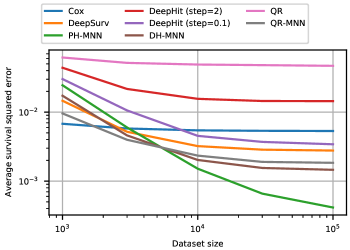
Figure 3: Averaged integrated squared error of the survival function for different dataset sizes. The results are the average of 100 independent models trained with independently generated datasets.

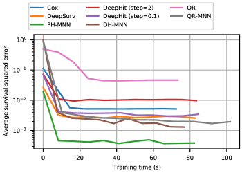
Figure 4: Averaged integrated squared error of the survival function over training time using a single synthetic dataset with 100000 data points. Computation was performed with a RTX 2070 graphics card and the models were implemented with TensorFlow 2.3.1.

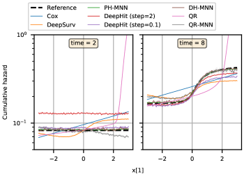
Figure 5: Cumulative cause-specific hazard function for event type $1$ in the synthetic data as a function of time and variable $x[1]$ when $x[0]=0$. The values estimated are the averaged over 100 independent models trained with independently generated datasets, each one with 100000 data points.

V Application to a clinical dataset

The proposed methodology was applied to the estimation of the risks of death and revision surgery for patients who undergo hip replacement surgery, using data collected by the National Joint Registry in the United Kingdom. This dataset contains outcomes information from 1132875 hip replacement surgeries performed from 2003 to 2019. Here, modeling was restricted to procedures performed from April 2009 to March 2019. Within this period, 855044 hip replacements were performed. The data was filtered to include only surgeries with complete data and only those where the reason for surgery was osteoarthritis, resulting in a total of 612914 procedures.

The observed population survival curves are shown in the Kaplan-Meier estimate [50]. The performance of the proposed MNN models, together with those of benchmark and current state-of-the-art approaches were compared against the observed Kaplan-Meier estimate. The models used for comparison were the same as in section IV. For the PH-MNN, the time knots used were 2, 4, and 7. For the DH-MNN and DeepHit, time knots were equally distributed in intervals of 6 months.

The models were evaluated with plots of the estimated cumulative hazard ratio (CHR) marginalized as a function of age and BMI. We chose age and BMI as example predictor variables as they demonstrate a nonlinear relationship with survival, which the proposed methods should be able to capture. The marginalized CHR estimation as a function of either the age or the BMI used a sliding window with width equal to 4 in respective units and centered successively in each target value, where:

• the Kaplan-Meier estimate of the survival function within the window was performed, $S_{KM}(t|x\in\xi(w))$, where $\xi(w)$ is a window centered in $w$;

• the marginal model estimate within the window is computed as the average of the estimated survival function for each patient within the window, $S_{model}(t|x\in\xi(w))$;

• the Kaplan-Meier estimate was computed for the entire test population, $S_{KM}(t)$;

• the Kaplan-Meier estimation of the marginal CHR was given by: $\frac{\log(S_{KM}(t|x\in\xi(w)))}{\log(S_{KM}(t))}$.

• the model estimation of the marginal CHR was given by: $\frac{\log(S_{model}(t|x\in\xi(w)))}{\log(S_{KM}(t))}$.

This process was repeated 250 times, for each model in a group of 50 random repetitions of 5-fold cross validation. The results of the estimated marginal CHR as a function of age or BMI averaged for all 250 runs are shown in Figs. 6-9. The results are evaluated according to the accuracy of representation of nonlinearities, adaptability of the shape as a function of time, and calibration. These three aspects are captured by the root mean square error of the model estimate of the log marginal CHR relative to the Kaplan-Meier estimate of the same quantity. For a given time $t$, this RMSE is given by:

$$RMSE=\frac{\int p(x\in\xi(w))\log^{2}\left(\frac{\log(S_{model}(t|x\in\xi(w)))}{\log(S_{KM}(t|x\in\xi(w)))}\right)\mathrm{d}w}{\int p(x\in\xi(w))\mathrm{d}w}$$ (14)

where $p(x)$ is the population density inside the window $\xi(w)$ centered in $w$, and $w$ is either the age or the BMI. This RMSE represents an integrated measure of two factors: first, the difference between the relationship of the model estimate and the observed data as a function of the attribute; and second the systematic bias between the two that is common for all values of the attribute. By estimating a bias that will minimize this RMSE, the two components can be identified as the unbiased RMSE (URMSE) and the bias. The model were evaluated through the computation of the RMSE, URMSE and absolute bias in the time interval from 6 months to 8 years with steps of 1 month. Tables I, II and III present for each type of model the maximum value over time of each evaluation criteria with their $95\%$ confidence interval. To highlight the improvement achieved with the metaparametric neural network structure, the results were grouped by type of model. For the direct hazards models, evaluation was performed in 6 months intervals to allow a fair comparison between both the discrete and continuous-time models.

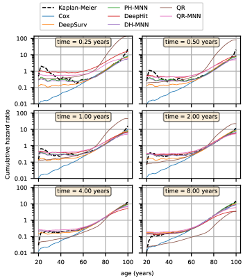
Figure 6: Estimated cumulative hazard ratio for the mortality risk marginalized as a function of the age.

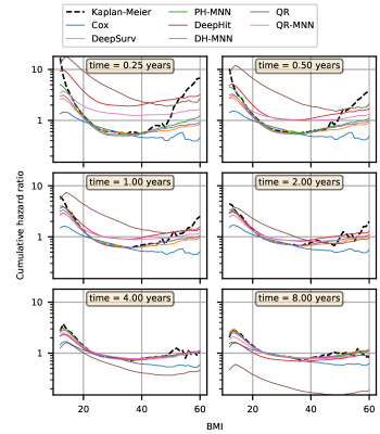
Figure 7: Estimated cumulative hazard ratio for the mortality risk marginalized as a function of the BMI.

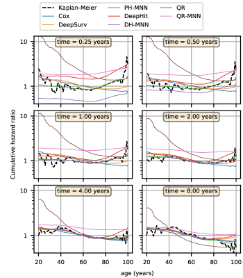
Figure 8: Estimated cumulative hazard ratio for the revision risk marginalized as a function of the age.

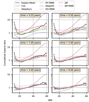
Figure 9: Estimated cumulative hazard ratio for the revision risk marginalized as a function of the BMI.

TABLE I: Maximum value over time of each error component in proportional hazards models

		Cox	DeepSurv	PH-MNN
Revision by Age	RMSE	$0.225\pm 0.002$	$0.213\pm 0.002$	$\mathbf{0.154\pm 0.003}$
	URMSE	$0.221\pm 0.003$	$0.209\pm 0.002$	$\mathbf{0.146\pm 0.002}$
	abs. bias	$0.060\pm 0.003$	$\mathbf{0.057\pm 0.003}$	$0.070\pm 0.002$
Mortality by Age	RMSE	$0.567\pm 0.002$	$0.313\pm 0.004$	$\mathbf{0.189\pm 0.004}$
	URMSE	$0.522\pm 0.002$	$0.279\pm 0.003$	$\mathbf{0.181\pm 0.004}$
	abs. bias	$0.243\pm 0.002$	$0.159\pm 0.003$	$\mathbf{0.071\pm 0.004}$
Revision by BMI	RMSE	$0.148\pm 0.002$	$0.140\pm 0.002$	$\mathbf{0.124\pm 0.002}$
	URMSE	$0.140\pm 0.001$	$0.130\pm 0.002$	$\mathbf{0.107\pm 0.002}$
	abs. bias	$0.074\pm 0.003$	$\mathbf{0.068\pm 0.003}$	$0.081\pm 0.002$
Mortality by BMI	RMSE	$0.197\pm 0.002$	$0.135\pm 0.002$	$\mathbf{0.133\pm 0.003}$
	URMSE	$0.193\pm 0.001$	$0.127\pm 0.002$	$\mathbf{0.121\pm 0.003}$
	abs. bias	$0.053\pm 0.003$	$\mathbf{0.052\pm 0.003}$	$0.061\pm 0.003$

TABLE II: Maximum value over time of each error component in direct hazards models

		DeepHit	DH-MNN
Revision by Age	RMSE	$0.456\pm 0.003$	$\mathbf{0.260\pm 0.004}$
	URMSE	$0.162\pm 0.002$	$\mathbf{0.148\pm 0.002}$
	abs. bias	$0.430\pm 0.002$	$\mathbf{0.217\pm 0.004}$
Mortality by Age	RMSE	$1.008\pm 0.004$	$\mathbf{0.228\pm 0.005}$
	URMSE	$0.194\pm 0.003$	$\mathbf{0.180\pm 0.004}$
	abs. bias	$0.990\pm 0.004$	$\mathbf{0.144\pm 0.005}$
Revision by BMI	RMSE	$0.444\pm 0.002$	$\mathbf{0.242\pm 0.003}$
	URMSE	$0.111\pm 0.002$	$\mathbf{0.107\pm 0.002}$
	abs. bias	$0.431\pm 0.002$	$\mathbf{0.218\pm 0.004}$
Mortality by BMI	RMSE	$0.990\pm 0.003$	$\mathbf{0.184\pm 0.005}$
	URMSE	$0.133\pm 0.002$	$\mathbf{0.120\pm 0.002}$
	abs. bias	$0.981\pm 0.003$	$\mathbf{0.140\pm 0.005}$

TABLE III: Maximum value over time of each error component in quantile regression models

		QR	QR-MNN
Revision by Age	RMSE	$0.697\pm 0.005$	$\mathbf{0.596\pm 0.052}$
	URMSE	$0.341\pm 0.003$	$\mathbf{0.171\pm 0.005}$
	abs. bias	$0.609\pm 0.005$	$\mathbf{0.570\pm 0.053}$
Mortality by Age	RMSE	$1.379\pm 0.005$	$\mathbf{0.576\pm 0.044}$
	URMSE	$0.730\pm 0.006$	$\mathbf{0.280\pm 0.011}$
	abs. bias	$1.364\pm 0.005$	$\mathbf{0.500\pm 0.045}$
Revision by BMI	RMSE	$\mathbf{0.595\pm 0.006}$	$0.598\pm 0.054$
	URMSE	$0.187\pm 0.002$	$\mathbf{0.154\pm 0.007}$
	abs. bias	$\mathbf{0.566\pm 0.006}$	$0.578\pm 0.054$
Mortality by BMI	RMSE	$1.682\pm 0.007$	$\mathbf{0.557\pm 0.039}$
	URMSE	$0.237\pm 0.003$	$\mathbf{0.176\pm 0.005}$
	abs. bias	$1.665\pm 0.007$	$\mathbf{0.515\pm 0.042}$

The PH-MNN, DH-MNN, QR-MNN, DeepSurv and DeepHit models captured the nonlinearities, while the Cox did not. The QR model partially captured some nonlinearities through the variation of coefficients with the quantile, but they were not entirely captured since this variation is shared to represent both nonlinearities and time variations. This can be seen in the figures and is reflected by a smaller URMSE for the neural network models in most cases. The nonlinearities of the CHR could be adapted as a function of time for all the metaparametric neural networks and for the DeepHit model. The model structure for the others does not permit this variation of nonlinearities over time.

In the case of the proportional hazards models, the PH-MNN overall performance measured by the RMSE was better than the established methods. When this RMSE measure is broken down into its components, URMSE and absolute bias, the DeepSurv model had a slightly smaller bias. However the PH-MNN bias was still small and stable across the different risks and attributes. For the direct hazards models, the DH-MNN overall performance, URMS and bias were all consistently better than DeepHit. Finally, for the quantile regression models, the QR-MNN model overall performance was also consistently better than the QR method, apart from revision by BMI in which the two methods were equivalent.

VI Conclusion

In this article, we propose a novel and generic framework for incorporating machine learning into survival modeling that resolves the established limitations of neural network application to this field. This MNN framework results in a structure that encompasses existing neural network models. This framework enables the generic representation of any survival probability distribution without prior knowledge of its functional form. The MNN framework can be applied to both parametric and semi-parametric modeling scenarios providing unification in this domain. Special instances of this class of models were formulated based on three different heritage structures: the proportional hazards, the quantile regression and the direct hazard. Both conventional and the novel framework models were evaluated using both a synthetic and a large real-world dataset, with best overall fit to the observed data being demonstrated by the proposed MNN framework.

References

- [1] P. S. Collaboration et al., “Age-specific relevance of usual blood pressure to vascular mortality: a meta-analysis of individual data for one million adults in 61 prospective studies,” The Lancet, vol. 360, no. 9349, pp. 1903–1913, 2002.
- [2] A. K. Clift, C. A. Coupland, R. H. Keogh, K. Diaz-Ordaz, E. Williamson, E. M. Harrison, A. Hayward, H. Hemingway, P. Horby, N. Mehta et al., “Living risk prediction algorithm (QCOVID) for risk of hospital admission and mortality from coronavirus 19 in adults: national derivation and validation cohort study,” BMJ, vol. 371, 2020.
- [3] E. Vasileiou, C. R. Simpson, C. Robertson, T. Shi, S. Kerr, U. Agrawal, A. Akbari, S. Bedston, J. Beggs, D. Bradley et al., “Effectiveness of first dose of COVID-19 vaccines against hospital admissions in scotland: national prospective cohort study of 5.4 million people,” 2021.
- [4] B. Pitt, F. Zannad, W. J. Remme, R. Cody, A. Castaigne, A. Perez, J. Palensky, and J. Wittes, “The effect of spironolactone on morbidity and mortality in patients with severe heart failure,” New England Journal of Medicine, vol. 341, no. 10, pp. 709–717, 1999.
- [5] S. E. Håberg, L. Trogstad, N. Gunnes, A. J. Wilcox, H. K. Gjessing, S. O. Samuelsen, A. Skrondal, I. Cappelen, A. Engeland, P. Aavitsland et al., “Risk of fetal death after pandemic influenza virus infection or vaccination,” New England Journal of Medicine, vol. 368, no. 4, pp. 333–340, 2013.
- [6] P. Aram, L. Trela-Larsen, A. Sayers, A. F. Hills, A. W. Blom, E. V. McCloskey, V. Kadirkamanathan, and J. M. Wilkinson, “Estimating an individual’s probability of revision surgery after knee replacement: A comparison of modeling approaches using a national dataset,” American Journal of Epidemiology, 2018.
- [7] N. M. Kiefer, “Economic duration data and hazard functions,” Journal of Economic Literature, vol. 26, no. 2, pp. 646–679, 1988.
- [8] J. M. Karpoff and X. Lou, “Short sellers and financial misconduct,” The Journal of Finance, vol. 65, no. 5, pp. 1879–1913, 2010.
- [9] J. Sikorska, M. Hodkiewicz, and L. Ma, “Prognostic modelling options for remaining useful life estimation by industry,” Mechanical Systems and Signal Processing, vol. 25, no. 5, pp. 1803–1836, 2011.
- [10] E. M. Liu, “Time to change what to sow: Risk preferences and technology adoption decisions of cotton farmers in China,” Review of Economics and Statistics, vol. 95, no. 4, pp. 1386–1403, 2013.
- [11] D. R. Cox, “Regression models and life-tables,” Journal of the Royal Statistical Society: Series B (Methodological), vol. 34, no. 2, pp. 187–202, 1972.
- [12] P. Royston and M. K. Parmar, “Flexible parametric proportional-hazards and proportional-odds models for censored survival data, with application to prognostic modelling and estimation of treatment effects,” Statistics in Medicine, vol. 21, no. 15, pp. 2175–2197, 2002.
- [13] J. Tang, C. Deng, and G.-B. Huang, “Extreme learning machine for multilayer perceptron,” IEEE Transactions on Neural Networks and Learning Systems, vol. 27, no. 4, pp. 809–821, 2015.
- [14] M. Bianchini and F. Scarselli, “On the complexity of neural network classifiers: A comparison between shallow and deep architectures,” IEEE Transactions on Neural Networks and Learning Systems, vol. 25, no. 8, pp. 1553–1565, 2014.
- [15] Z.-Q. Zhao, P. Zheng, S.-t. Xu, and X. Wu, “Object detection with deep learning: A review,” IEEE Transactions on Neural Networks and Learning Systems, vol. 30, no. 11, pp. 3212–3232, 2019.
- [16] K. Greff, R. K. Srivastava, J. Koutník, B. R. Steunebrink, and J. Schmidhuber, “LSTM: A search space odyssey,” IEEE Transactions on Neural Networks and Learning Systems, vol. 28, no. 10, pp. 2222–2232, 2016.
- [17] R. G. Miller, “Least squares regression with censored data,” Biometrika, vol. 63, no. 3, pp. 449–464, 1976.
- [18] J. Buckley and I. James, “Linear regression with censored data,” Biometrika, vol. 66, no. 3, pp. 429–436, 1979.
- [19] L. Peng and Y. Huang, “Survival analysis with quantile regression models,” Journal of the American Statistical Association, vol. 103, no. 482, pp. 637–649, 2008.
- [20] T. Moreau, J. O’quigley, and M. Mesbah, “A global goodness-of-fit statistic for the proportional hazards model,” Journal of the Royal Statistical Society: Series C (Applied Statistics), vol. 34, no. 3, pp. 212–218, 1985.
- [21] R. J. Gray, “Flexible methods for analyzing survival data using splines, with applications to breast cancer prognosis,” Journal of the American Statistical Association, vol. 87, no. 420, pp. 942–951, 1992.
- [22] T. Hastie and R. Tibshirani, “Varying-coefficient models,” Journal of the Royal Statistical Society: Series B (Methodological), vol. 55, no. 4, pp. 757–779, 1993.
- [23] W. Sauerbrei, C. Meier-Hirmer, A. Benner, and P. Royston, “Multivariable regression model building by using fractional polynomials: description of SAS, STATA and R programs,” Computational Statistics & Data Analysis, vol. 50, no. 12, pp. 3464–3485, 2006.
- [24] R. L. Prentice, J. D. Kalbfleisch, A. V. Peterson Jr, N. Flournoy, V. T. Farewell, and N. E. Breslow, “The analysis of failure times in the presence of competing risks,” Biometrics, pp. 541–554, 1978.
- [25] M. G. Larson and G. E. Dinse, “A mixture model for the regression analysis of competing risks data,” Journal of the Royal Statistical Society: Series C (Applied Statistics), vol. 34, no. 3, pp. 201–211, 1985.
- [26] J. P. Fine and R. J. Gray, “A proportional hazards model for the subdistribution of a competing risk,” Journal of the American Statistical Association, vol. 94, no. 446, pp. 496–509, 1999.
- [27] S. Choi, L. Zhu, and X. Huang, “Semiparametric accelerated failure time cure rate mixture models with competing risks,” Statistics in Medicine, vol. 37, no. 1, pp. 48–59, 2018.
- [28] D. Faraggi and R. Simon, “A neural network model for survival data,” Statistics in Medicine, vol. 14, no. 1, pp. 73–82, 1995.
- [29] J. L. Katzman, U. Shaham, A. Cloninger, J. Bates, T. Jiang, and Y. Kluger, “DeepSurv: personalized treatment recommender system using a Cox proportional hazards deep neural network,” BMC Medical Research Methodology, vol. 18, no. 1, p. 24, 2018.
- [30] X. Zhu, J. Yao, and J. Huang, “Deep convolutional neural network for survival analysis with pathological images,” in IEEE International Conference on Bioinformatics and Biomedicine. IEEE, 2016, pp. 544–547.
- [31] F. Kiaee, H. Sheikhzadeh, and S. E. Mahabadi, “Relevance vector machine for survival analysis,” IEEE Transactions on Neural Networks and Learning Systems, vol. 27, no. 3, pp. 648–660, 2015.
- [32] P. Chapfuwa, C. Tao, C. Li, C. Page, B. Goldstein, L. C. Duke, and R. Henao, “Adversarial time-to-event modeling,” in International Conference on Machine Learning. PMLR, 2018, pp. 735–744.
- [33] H. Ishwaran and M. Lu, “Random survival forests,” Wiley StatsRef: Statistics Reference Online, pp. 1–13, 2008.
- [34] H. Ishwaran, T. A. Gerds, U. B. Kogalur, R. D. Moore, S. J. Gange, and B. M. Lau, “Random survival forests for competing risks,” Biostatistics, vol. 15, no. 4, pp. 757–773, 2014.
- [35] G. Chen, “Nearest neighbor and kernel survival analysis: nonasymptotic error bounds and strong consistency rates,” in International Conference on Machine Learning, 2019, pp. 1001–1010.
- [36] C.-N. Yu, R. Greiner, H.-C. Lin, and V. Baracos, “Learning patient-specific cancer survival distributions as a sequence of dependent regressors,” in Advances in Neural Information Processing Systems, 2011, pp. 1845–1853.
- [37] C. Lee, W. R. Zame, J. Yoon, and M. van der Schaar, “Deephit: a deep learning approach to survival analysis with competing risks,” in Association for the Advancement of Artificial Intelligence Conference, 2018.
- [38] K. Ren, J. Qin, L. Zheng, Z. Yang, W. Zhang, L. Qiu, and Y. Yu, “Deep recurrent survival analysis,” in Association for the Advancement of Artificial Intelligence Conference, 2019, pp. 1–8.
- [39] S. Martino, R. Akerkar, and H. Rue, “Approximate Bayesian inference for survival models,” Scandinavian Journal of Statistics, vol. 38, no. 3, pp. 514–528, 2011.
- [40] H. Joensuu, A. Vehtari, J. Riihimäki, T. Nishida, S. E. Steigen, P. Brabec, L. Plank, B. Nilsson, C. Cirilli, C. Braconi et al., “Risk of recurrence of gastrointestinal stromal tumour after surgery: an analysis of pooled population-based cohorts,” The Lancet Oncology, vol. 13, no. 3, pp. 265–274, 2012.
- [41] T. Fernández, N. Rivera, and Y. W. Teh, “Gaussian processes for survival analysis,” in Advances in Neural Information Processing Systems, 2016, pp. 5021–5029.
- [42] A. M. Alaa and M. van der Schaar, “Deep multi-task Gaussian processes for survival analysis with competing risks,” in Advances in Neural Information Processing Systems, 2017, pp. 2326–2334.
- [43] R. Ranganath, A. Perotte, N. Elhadad, and D. Blei, “Deep survival analysis,” in Machine Learning for Healthcare Conference. PMLR, 2016, pp. 101–114.
- [44] X. Miscouridou, A. Perotte, N. Elhadad, and R. Ranganath, “Deep survival analysis: nonparametrics and missingness,” in Machine Learning for Healthcare Conference, 2018, pp. 244–256.
- [45] D. R. Wilson and T. R. Martinez, “The general inefficiency of batch training for gradient descent learning,” Neural Networks, vol. 16, no. 10, pp. 1429–1451, 2003.
- [46] J. Kalbfleisch and R. L. Prentice, Statistical analysis of failure time data. Wiley, 1980.
- [47] N. Breslow, “Covariance analysis of censored survival data,” Biometrics, pp. 89–99, 1974.
- [48] Q. Zheng, L. Peng, X. He et al., “High dimensional censored quantile regression,” The Annals of Statistics, vol. 46, no. 1, pp. 308–343, 2018.
- [49] N. Srivastava, G. Hinton, A. Krizhevsky, I. Sutskever, and R. Salakhutdinov, “Dropout: a simple way to prevent neural networks from overfitting,” The Journal of Machine Learning Research, vol. 15, no. 1, pp. 1929–1958, 2014.
- [50] E. L. Kaplan and P. Meier, “Nonparametric estimation from incomplete observations,” Journal of the American Statistical Association, vol. 53, no. 282, pp. 457–481, 1958.