Artificial Neural Network classification of asteroids in the M1:2 mean-motion resonance with Mars

Abstract

Artificial neural networks (ANN) have been successfully used in the last years to identify patterns in astronomical images. The use of ANN in the field of asteroid dynamics has been, however, so far somewhat limited. In this work we used for the first time ANN for the purpose of automatically identifying the behaviour of asteroid orbits affected by the M1:2 mean-motion resonance with Mars. Our model was able to perform well above 85% levels for identifying images of asteroid resonant arguments in term of standard metrics like accuracy, precision and recall, allowing to identify the orbital type of all numbered asteroids in the region. Using supervised machine learning methods, optimized through the use of genetic algorithms, we also predicted the orbital status of all multi-opposition asteroids in the area. We confirm that the M1:2 resonance mainly affects the orbits of the Massalia, Nysa, and Vesta asteroid families.

1 Introduction

During the last five years, machine learning and deep learning have been more and more been used in the field of asteroid dynamics. Among the latest application, supervised methods of machine learning have been used to identify the population of asteroids in three-body mean-motion resonances (Smirnov & Markov, 2017), new members of known asteroid families (Carruba et al., 2020), and asteroids groups inside the $z_{1}$ and $z_{2}$ secular resonances (Carruba et al., 2021), among others. Deep learning in the form of artificial neural networks has been recently used for identifying members of asteroid families (Vujičić et al., 2020). While several applications of artificial neural networks exist in other astronomy fields for the purpose of identifying images, like, for instance, methods to identify different types of galaxies clusters (Su et al., 2020), to our knowledge such methods have not yet been applied for asteroid dynamics problems.

Here we attempt for the first time to use artificial neural networks for automatically identifying the behaviour of asteroids near the two-body M1:2 mean-motion resonance with Mars. As discussed by other authors (Gallardo et al., 2011), three types of orbits are possible near resonance: libration, where the resonant argument of the resonance, which we will define in section (2), oscillates around an equilibrium point, circulation, where the resonant argument cover the whole range of values from $0^{\circ}$ to $360^{\circ}$, and switching orbits, where the resonant argument alternates phases of libration and circulation. In previous works, the classification of the type of orbits on which an asteroid resides was either performed manually, by visually inspecting the time behaviour of the resonance argument (see, for instance, Carruba et al. (2018) and references therein), or by using automatic algorithms for the same purpose (Smirnov et al., 2018; Gallardo, 2014; Gallardo et al., 2016). In this work, we use artificial neural networks for classifying an asteroid’s orbital type for all numbered asteroids in the region affected by this resonance.

We then employed genetic algorithms to select the best performing machine learning supervised method, to predict the labels of multi-opposition objects in the area. Multi-opposition asteroids are asteroids that have been observed at several oppositions to the Sun from Earth, whose orbits are somewhat well-established. Once the orbit is confirmed, an asteroid receives an identification number and becomes a numbered asteroid, like 2 Vesta, 4 Pallas, 10 Hygiea, among others. Since the orbits of multi-oppositions asteroids are not as well-established as those of numbered bodies, here we used the labels of numbered asteroids to predict those of the multi-oppositions objects. Finally, we verified which local asteroid families are most affected by this dynamical resonance, to see if our results are consistent with those in the literature. We start our analysis by revising the dynamical properties of asteroids in the region.

2 The population of asteroids in the M1:2 resonance: dynamics

The population of asteroids inside the M1:2 mean motion resonance with Mars has been the subject of a study by Gallardo et al. (2011), that investigated the dynamical, physical and evolutionary properties of these asteroids. Here we will briefly summarize the dynamical characteristics of this population, and distinguish between the types of orbits possible in the orbital region affected by this resonance. Figure (1) displays an $(a,e)$ projection of 9457 numbered asteroids in the range in $a$ from 2.411 to 2.426 au. Values of synthetic proper elements for asteroids in the region were obtained from the Asteroid Families Portal ($AFP$, Radović et al. (2017), accessed on August 1st, 2020). Synthetic proper elements are constant of the motion on timescales of millions of years and are obtained as the outcome of numerical simulations, using methods described in Knežević & Milani (2003). The V-shaped region at the resonance centre is associated with the M1:2 resonance. The higher number concentration of objects at the edge of the V-shape is caused by the phenomenon called “resonance stickiness” (Malyshkin & Tremaine, 1999). Gallardo et al. (2011) define two main resonant arguments for this resonance. $\sigma$ is given by:

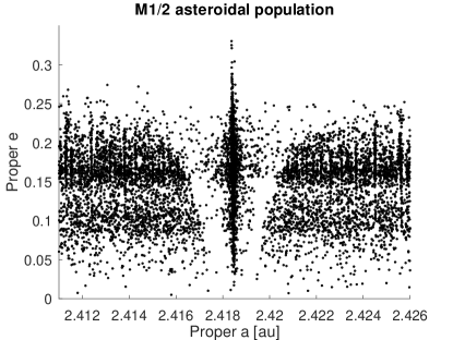
Figure 1: Proper $(a,e)$ distribution for asteroids in the orbital region of the M1:2 mean-motion resonance.

$$\sigma=2\lambda-{\lambda}_{M}-\varpi,$$ (1)

where $\lambda=M+\Omega+\omega$ is the mean longitude, $\varpi=\Omega+\omega$, with $\Omega$ the longitude of the node, $\omega$ the argument of pericentre, and where the suffix $M$ identifies the planet Mars. ${\sigma}_{1}$ is defined as:

$${\sigma}_{1}=2\lambda-{\lambda}_{M}-{\varpi}_{M}.$$ (2)

The orbital behaviour of asteroids in the affected region can be identified by studying the time dependence of these two angles. As previously discussed, asteroids for which the critical arguments cover the whole range of values, from $0^{\circ}$ to $360^{\circ}$, are on circulating orbits. If the argument oscillates around an equilibrium point we have a librating orbit. Whether the argument alternates phases of libration and circulations, or switch between different equilibrium points, we have a switching orbit, as defined in this work. We identify the orbital types of asteroids by performing a 100000 yr simulation with the Burlisch-Stoer integrator of the SWIFT package (Levison & Duncan, 1994). We use a time step of 1 day, a tolerance ($EPS$) equal to $10^{-8}$, and integrated the asteroids under the influence of all planets. None of the asteroids in our sample is a Mars-crosser or susceptible to experience close encounters with planets, which justifies the use of a Burlisch-Stoer integrator for this study. Figure (2) show the resonant argument for three asteroids in each of the three classes. As discussed by Gallardo et al. (2011), since the M1:2 is an external resonance, unusual equilibrium points for the $\sigma$ argument, like one at $100^{\circ}$, can occur. The main equilibrium point for the ${\sigma}_{1}$ argument is around $0^{\circ}$.

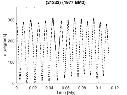
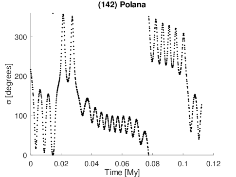
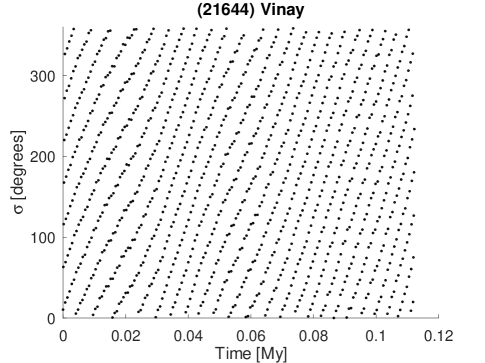
Figure 2: The resonant angles $\sigma$, as defined by equation (1) as a function of time for asteroids on librating, switching and circulating orbits of the M1:2 resonance.

Using this simulation set-up, we integrated 1000 asteroids in the orbital region of the M1:2 mean-motion resonance. Figure (3) shows an $(a,e)$ projection of these asteroids, colour-coded for the behaviour of the $\sigma$ (left panel) and ${\sigma}_{1}$ resonant argument. The main difference between the two cases is the fraction of asteroids in pure librating states. For the case of $\sigma$, there were just 4 librators (0.4%) and 202 oscillators (20.2). For ${\sigma}_{1}$, there were 69 librators (6.9%) and 185 oscillators (18.5%). Pure $\sigma$ librators tend to be much rarer than pure ${\sigma}_{1}$ ones. Since in this work we are interested in treating a multi-class problem, rather than a binary one, from now on we will focus our study on the case of the ${\sigma}_{1}$ resonant arguments.

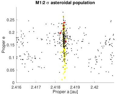
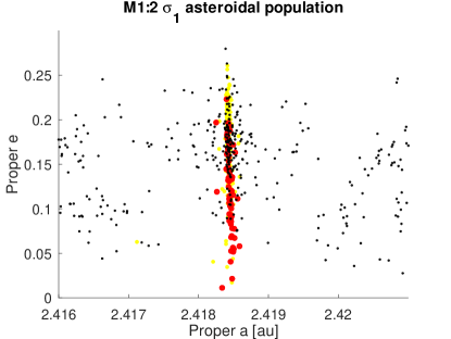
Figure 3: A proper $(a,e)$ projection of asteroids in the region of the M1:2 resonance. The left panel shows the orbital behaviour for the $\sigma$ resonant argument colour-coded as follows: red full circles are librators, yellow full circles are oscillators, and black dots are circulators. The right panel does the same, but for the ${\sigma}_{1}$ resonant argument.

3 Artificial Neural Networks

At the time that we carried out this study, there were 6440 numbered and multi-opposition asteroids in the region of the M1:2 mean-motion resonance. Analyzing resonant arguments for each of the asteroids in the region may be a very tiring and time-consuming endeavour, if performed manually. Automatic approaches not based on machine-learning have been developed in the last years to solve this problem (Smirnov et al., 2018; Gallardo, 2014; Gallardo et al., 2016). Here this task will be performed by using artificial neural networks (ANN). The human brain classifies images by converting the light received by the eye’s retina into electrical signals, that are then processed by a hierarchy of connected neurons to identify patterns.

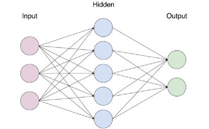
Figure 4: A simple architecture for an Artificial Neural Network. The network has 3 neurons in the input layer, 5 in the hidden one and two in the output layer.

Artificial neuron networks mimic the neurons web in a biological brain. Each artificial neuron can transmit a signal to other neurons. This signal, which is usually a real number, can be processed, and the signal coming out of each neuron is computed as a non-linear function of the inputs. A basic architecture for ANN consists of an input and an output layers, with the possible presence of one or more hidden layers between them to improve the model precision. Generally speaking, input layers will look for simpler patterns, while output layers will search for more complex relationships. Figure (4) shows the architecture of a simple ANN, with 3 neurons in the input layer, 5 in the hidden stratus, and 2 in the output layer. Each neuron will perform a weighted sum, $W_{S}$, given by:

$$W_{S}=\sum_{i=1}^{n}w_{i}X_{i},$$ (3)

where n is the number of input to process, $X_{i}$ are the signals from other neurons, and $w_{i}$ are the weights. ANN will optimize the values of the weights during the learning process. On the weighted sum $W_{S}$, ANN will apply an activation function. For images classifications, one of the most used activation function is the “relu”, defined as:

$$y=max(W_{S},0),$$ (4)

which will produce as an outcome the weighted sum itself $W_{S}$, if that is a positive number, or 0, if $W_{S}$ has a negative value. As a next step, the loss function must be applied to all the weights in the network through a back-propagation algorithm. A loss function is usually calculated by computing the differences between the predicted and real output values. An example of a loss function is the mean squared error, defined as:

$$C=\frac{1}{2}\sum_{j=1}^{n}(y_{j}-{\overline{y}}_{j})^{2},$$ (5)

where ${\overline{y}}_{j}$ is the expected value of the j-th outcome. For classification problems with multiple classes, with single classes identified by numbers, like the problem that we will discuss in this paper, the sparse_categorical_crossentropy loss function is generally used. Interested readers can find more information on the definition and use of this and other loss functions in the Keras documentation (https://keras.io/, Chollet & others (2018)). Once the loss function has been computed, the next step is to find its minimum, to optimize the values of the weights. Optimization algorithms find the gradient of the loss function and update the weights in the ANN based on this result. In this work, we will use the Adam optimizer (Kingma & Ba, 2015).

ANN use initial values of weights near zero. The first row of data is provided as input and processed through the network. The prediction of the network is compared to the real result, and the optimization of the cost function updates the values of the weights. This procedure is then repeated for all data, or, in some cases, for a subset, also called batch. An epoch is completed when the training procedure is finished for all the observations. This whole process can then be repeated for other epochs, to improve the quality of the predictions.

Interested readers could find more information about the use of ANN in artificial intelligence in (Lecun et al., 2015), or in the recent work on the application of ANN to the identification of asteroids belonging to asteroid families by (Vujičić et al., 2020), and references therein. In the next subsection we will discuss applications of ANN for the classification of images.

3.1 Applications of ANN to M1:2 resonant arguments images

Here we used the Keras implementation of ANN, which is also based on the Tensorflow Python software package (Chollet & others, 2018). The process used in this work is the following:

1. The asteroid orbits are integrated under the gravitational influences of the planets.

2. We compute the resonant arguments

3. Images of the time dependence of resonant arguments are drawn

4. The ANN trains on the training label image data

5. Predictions on the test images are obtained, and images of the test data, with their classification are produced.

The last step of producing images for the test data, with the proposed classification, is performed to make a visual confirmation by the user easier. The theory behind steps (i) and (ii) was discussed in section (2). Here we will focus on steps (iii), (iv) and (v). 100$\times$ 100 pixel images of resonant arguments of the M1:2 resonance were stored and pre-processed before applying our model in step (iii). Each image pixel values fall in the range from 0 to 255. Before feeding the images to our model, we normalized the pixel values to a range between zero and one, to help the ANN to learn faster. The choice of the image resolution was a compromise between not exceeding the computer memory available in our machines while still having a resolution sufficient for the ANN to successfully work.

To identify resonant argument images, we created a four-layer model with a flatten, an inner, a hidden, and an output layers. The architecture of the model is displayed in figure (5). The flatten layer will transform the image matrices into arrays. The inner layer will look for simpler patterns in the arguments images, while the hidden layer, with half the neurons of the inner one, will search for more complex features. The output layer, with three nodes, will perform the final classification for the three possible classes: circulation, switching and librating orbits.

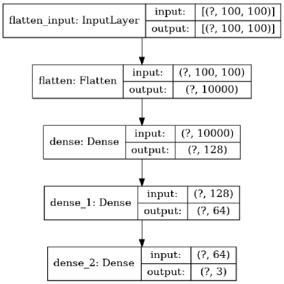
Figure 5: Neural network structure of the model used for classifying resonant arguments. We used a flatten layer, an inner layer, a hidden layer, and an output layer for final classification.

To quantitatively classify the outcome of ANN, it is often useful to compute values of metrics. Some of the most commonly used metrics for classifications problems are the accuracy, recall and precision. For a given class of orbits, we define True-Positive (TP) as the number of images successfully identified as belonging to that class by both the observer and the ANN model. True-Negative (TN) are the number of images that both methods identify as non-belonging to a given class. False-Positive (FP) are images classified as belonging to a class just by the ANN method. Finally, False-Negative (FN) are the images not classified to belong to a class just by the ANN approach. Values of $TP,TN,FP$ and $FN$ can be obtained by computing the confusion matrix on the images real and predicted labels. With these definitions, $accuracy$ (Fawcett, 2006) is given by:

$$accuracy=\frac{TP+TN}{TP+TN+FP+FN},$$ (6)

Recall, also known as Completeness in Carruba et al. (2020), is given by:

$$Completeness=\frac{TP}{TP+FN},$$ (7)

Precision, also known as Purity in Carruba et al. (2020), is defined as:

$$Purity=\frac{TP}{TP+FP}.$$ (8)

While accuracy can yield information on the efficiency of the algorithm as a whole, Completeness may inform on the ability of the method to efficiently retrieve the actual population of a given class, while Purity is related to the ability of the model not to include too many false positives ($FP$). The optimal model should be trained to give a trade-off between values of Completeness and of Purity. Carruba et al. (2020) recently introduced a Merit metrics that can automatically perform this trade-off, by giving larger weight to Purity. This new metrics is defined as:

$$Merit=\frac{1}{\sqrt{5}}\sqrt{{(Completeness)}^{2}+4\times{(Purity)}^{2}}.$$ (9)

In Carruba et al. (2020), a higher weight was given to Purity with respect to Completeness because this metric was more relevant to that work. Different definitions of Merit can be made, depending on the type of problem to be studied.

As discussed in section (3), the training of ANN can be performed for an arbitrary number of times, or epochs, to optimize the quality of the predictions. Figure (6) displays a plot of accuracy, as defined by equation (6) as a function of epoch for the training of a neural network with a training set of 1000 images and a test set of 200 images. Values of accuracy improve as a function of time, but there may be fluctuations from one epoch to the other, as shown in figure (6) for epochs 12 to 13, and 22 to 23. To avoid using non-optimal weights for the ANN, we use a callback instruction, as implemented by Keras, during the training to save the weights of each model, and automatically upload for the model predictions the weights associated with the best outcome in term of accuracy.

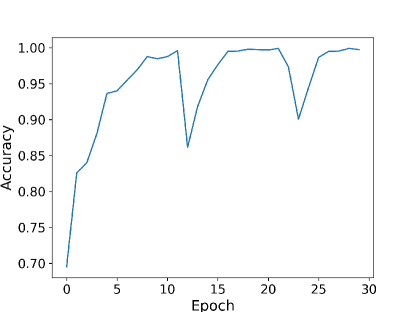
Figure 6: Dependence of accuracy as a function of epoch.

As a final step, we predicted the label of each image using the best model found with the procedures previously described. A set of 50 images with their predicted labels is shown in figure (7). Percentage values show the confidence level with which the model can classify the images. For the case of this set of images, the model accurately predicted the labels of 42 images and misread 8. 5 images of switching orbits were classified as circulation cases, and 3 circulating orbits were labeled as switching ones. All the libration cases were correctly identified. Values of the Merit metric for libration, switching and circulation images were 1.000, 0.755, and 0.877, respectively.

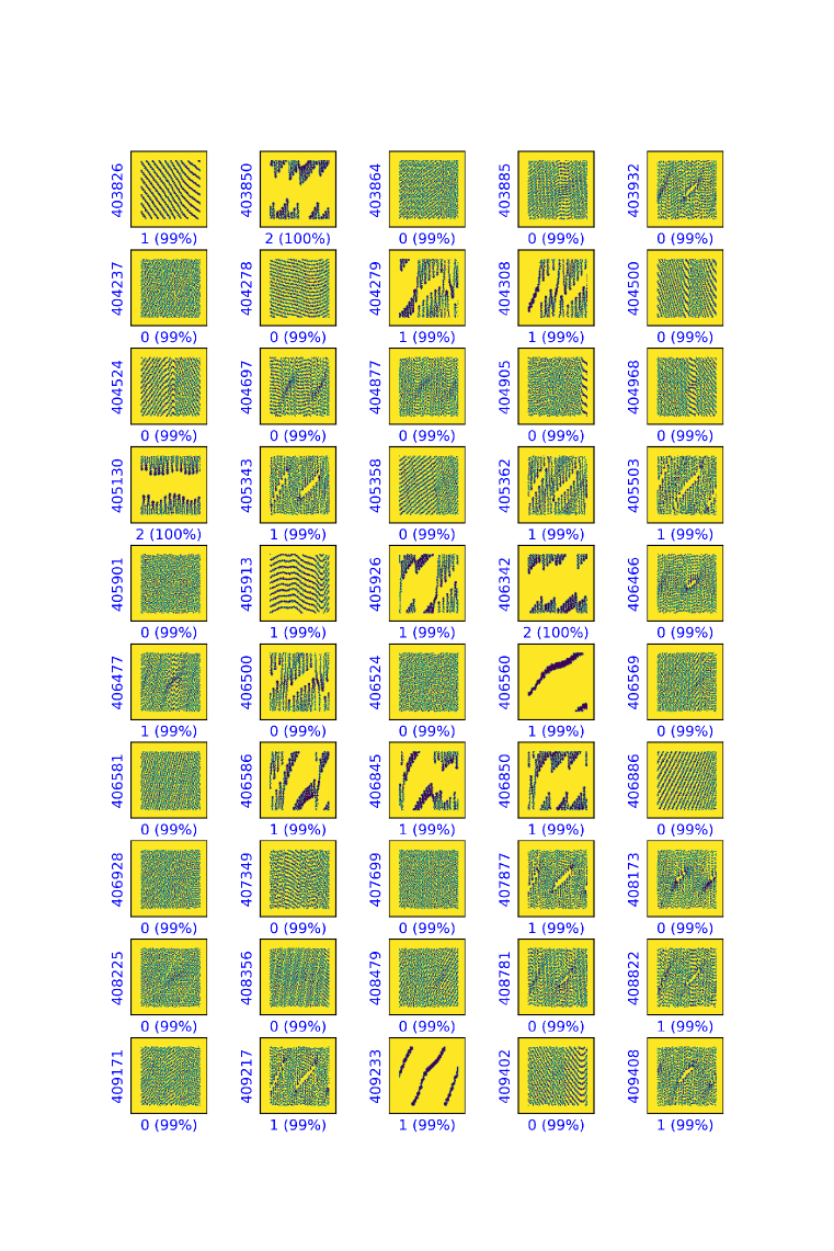
Figure 7: A set of 50 images with the prediction from the ANN model. The percentage values identify the confidence level with which the model classifies the images.

As a general rule in machine learning, the greater the size of the training sample, the better the model performance. Classification of images with ANN usually requires a training sample of the order of 60000 images (see, for instance, the example of clothes images classification using the Fashion MNIST data-set in the Keras documentation pages Chollet & others (2018)). For the case of the M1:2 asteroidal population, this is simply not viable, since there are just 5700 numbered asteroids in the range of $a$ near the resonance ($2.411<a<2.426$ au), i.e., an order of magnitude less. Yet, despite this fundamental limitation, our model performs quite well. To quantitatively estimate its efficiency, we computed values of our metrics, Completeness, Purity and Merit, for the same set of 50 images of M1:2 resonant arguments, increasing the size of the training set. Values of these metrics were computed for the three different types of orbits, libration, switching and circulation. For all the simulations, Accuracy values were all above 0.996.

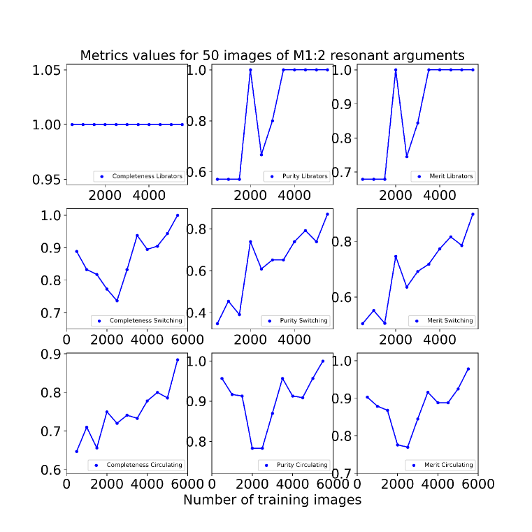
Figure 8: Values of Completeness, Purity and Merit for a set of 50 images of M1:2 resonant arguments for asteroids on librating, switching, and circulating orbits. The labels in each of the nine panels identify the metric value for each figure.

Figure (8) displays our results. Since the results of ANN are inherently stochastic, individual data point can change if we repeat the numerical experiment. But the overall trends should be robust. The model Merit improves in all cases for increasing values of the size of the training set. The model can more easily identify images of librating asteroids, since they are more distinguished from the other classes of orbits. Values of Merit reach 1.00 already for a training sample of 3500 images. The lowest performance was obtained for switching orbits, which are easier to be confused with the other two classes. However, even for this kind of orbits, the model could achieve values of Merit larger than 0.80, if a sample large enough ($>4500$ images) is used. Overall, ANN can be used to provide a preliminary classification of asteroids resonant arguments, with good results.

4 Applications of genetic algorithms to M1:2 resonant arguments labels

The next step of our analysis would be to predict the labels of asteroids near the M1:2 resonance based on their proper elements distribution and the labels of an appropriate training sample. For this purpose, we can either use a machine learning algorithm or an ANN. As discussed in the previous section, ANN become competitive with standard machine learning approaches for large sizes of the training sample, which is not the case for our problem. A possible application of ANN, and its limitations, will be discussed in section (4.1). Here, we will focus our attention on standard machine learning approaches.

Machine learning methods, either if standalone, where a single algorithm is applied, or ensemble methods, where several algorithms are combined, depend on several model parameters, or hyper-parameters. For instance, Random Forest methods that use several single Decision Trees depend on the number of trees used, which is a hyper-parameter that needs to be optimized. Identifying the optimal machine learning method and the combination of hyper-parameters for a given problem may be a long and time-consuming process. Here, as done in Carruba et al. (2021) for the case of asteroids near the $z_{1}$ and $z_{2}$ secular resonances, we use an approach based on genetic algorithms (Chen et al., 2004).

Genetic algorithms use an approach based on genetic evolution. First, several models and their related combinations of hyper-parameters are created. After an iteration of the model, also called generation, a scoring function can be used to identify the best models. Models similar to the best ones can then be created, and the process can be repeated until some conditions are satisfied. Interested readers can found more details on this procedure in (Chen et al., 2004) and (Carruba et al., 2021). As in the last paper, we used the Tpot Python library (Trang et al., 2019; Olson et al., 2016) with 5 generations, a population size (the number of models to keep after each generation) of 20, and a cross-validation cv equal to 5. We also used thee values of the random state: 42, 99, and 122, which correspond to three different models: XGBoost, GBoost, and Random Forest. The specifications of the best among these models will be discussed later on in this section.

To test these models we divided our sample of 5700 labelled asteroids into three parts: a training set of 200 asteroids, a test set of 200 bodies, and a pooling sample with the rest of the labelled objects. The size of the test sample is large enough for the results to be statistically significant (3.51% of the available data), but small enough to leave space for enough data in the initial training and pooling sample. A random asteroid is selected in the pooling sample, added to the training set, and the model is fitted to the test sample. Values of the metrics are computed, and the procedure is then repeated until there are no more objects in the pooling sample. Figure (9) displays the values of Completeness, Purity, and Merit for the switching orbits class, the type of orbits that previous analysis showed to be the most difficult to predict, obtained by the best model among the tested ones, the Random Forest algorithm. This model and its hyper-parameters are discussed in appendix 1.

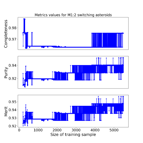
Figure 9: Values of Completeness, Purity and Merit for test labelled asteroids on switching orbits as a function of the training sample size, obtained with the Random Forest algorithm.

The Random Forest reaches a plateau in values of Completeness, Purity, and Merit for a training size of $\simeq 3000$. We will use this model to predict the labels of unlabelled asteroids in section (5)

4.1 Applications of ANN

ANN can also be applied to predict the labels of near resonance asteroids. However, as previously discussed the training sample available for this problem is too small for this method to be used advantageously. We created a three-layered Keras model with an inner layer of 200 neurons, one each for the asteroids in the test sample, a hidden layer of 100 neurons, i.e. 50% of the number of neurons in the inner layer, as it is usually recommended, and an outer layer of 3 neurons, one for each orbital-class. We choose to work with a training sample of 5500 asteroids and a test sample of 200, to have a large training sample, with 96.5% of the available data. Other choices for size of the test sample are, of course, possible. We expect, however, that the model results should be inferior for smaller sizes of the training sample. We run this model over 100 epochs with a callback instruction, to identify the labels of the same test sample used in section (4). The model was not able to identify librating asteroids, and values of Completeness, Purity and Merit for circulating and switching orbits were consistently below what predicted using genetic algorithms. Given these considerations, we will not use ANN to predict labels of unlabelled asteroids hereafter.

5 Identification of resonant groups

Having identified the best performing supervised learning algorithm in section (4), here we use this method to predict the labels of 740 multi-opposition asteroids, obtained from the $AFP$, using the 5700 asteroids that we previously classified as a training set. Figure (10) displays a proper $(a,e)$ projection of 6440 asteroids for which we obtained labels, using the same colour code as in figure (3). The predicted labels are very consistent with those obtained in the preliminary analysis, which confirms the validity of our method.

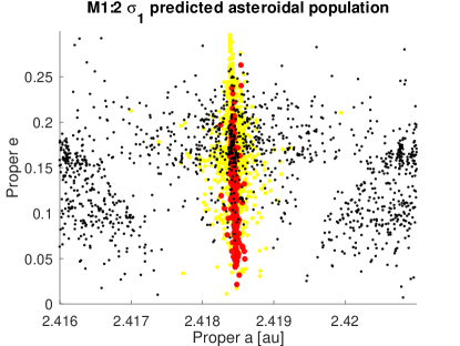
Figure 10: A proper $(a,e)$ projection of asteroids in the region of the M1:2 resonance. The colour code of predicted and confirmed asteroids in the region is the same as that of figure (3).

As a final check, we searched for possible dynamical clusters in the populations of M1:2 asteroids on librating and switching orbits, to see if our results are consistent with those in the literature. Gallardo et al. (2011) found that the three asteroids families most affected by the M1:2 mean-motion resonance were those of Nysa, Massalia, and Vesta. Here, following the approach of Carruba et al. (2021), we use learning Hierarchical Clustering Method (HCM), as implemented in Carruba et al. (2019), on a domain of proper elements for the group of M1:2 asteroids above described. The procedure used to implement this method was the same as that applied in Carruba et al. (2021): a critical distance cutoff $\frac{1}{2}d_{0}$ was obtained, and groups were identified for values of $d_{0}\pm 5$ m/s. We then verified if members of groups identified in this domain were listed as members of a family by Milani et al. (2014) and Nesvorný et al. (2015). Please note that Milani et al. (2014) reports the Nysa family as Hertha. Our results are summarized in table (1). We selected groups that have at least 10 members at the critical distance cutoff value, 5 members at the lowest distance cutoff of $d_{0}-5=22.75$ m/s, and were still identifiable at the highest distance cutoff of $d_{0}-5=32.75$ m/s. Interested readers could find more details on the procedures used in Carruba et al. (2019, 2021).

Table 1: The table reports the dynamical groups with at least 10 members among the librating and switching M1:2 population, listed from the most to the least numerous, identified with the hierarchical clustering algorithm, at three values of the distance cutoff: (1) 22.75, (2) 27.75, and (3) 32.75 m/s. The fourth column reports how many of the asteroids belong to a known asteroid family.

Family	Number of	Number of	Number of	Family members
Id.	members (1)	members (2)	members (3)	with known fam. ID.
19205 (1992 PT)	8	50	84	Massalia: 28, Nysa:3
42462 (5278 T-3)	13	19	25	Massalia: 13, Nysa:1
120135 (2003 GF7)	10	17	28	Nysa: 2
95459 (2002 CF307)	8	14	18	Vesta: 2
44931 (1999 VD39)	7	10	10	Nysa: 4
73066 (2002 FV15)	8	10	40	Massalia: 8
10516 Sakurajima	6	10	15	Nysa: 5, Massalia:1

Our analysis produced seven possible groups, all associated with the Massalia, Nysa, and Vesta families, so confirming the analysis of Gallardo et al. (2011).

6 Conclusions

The main result of this work is the use of ANN for identifying the behaviour of M1:2 resonant arguments images. It is the first time, to our knowledge, that ANNs have been used for such purpose in the field of asteroid dynamics. The use of this model allowed us to classify the orbital type of all numbered asteroids in the orbital region affected by this resonance, which has also been independently confirmed by a visual analysis by all authors.

The labels for the population of numbered asteroids near the M1:2 mean-motion resonances were also used to predict the orbital status of multi-opposition asteroids. Using genetic algorithms, we identify the best performing supervised learning method for our data, that we used to obtain labels for asteroids, without the need to perform a numerical simulation and an analysis of resonant angles.

The identification of clusters in the population of asteroids in librating and switching orbits suggested that three asteroid families, those of Massalia, Nysa, and Vesta, are the most dynamically affected by this resonance, so confirming the analysis of previous authors (Gallardo et al., 2011).

The methods developed in this work could be easily used for other cases of asteroids affected by mean-motion resonance, like the ones studied by Smirnov & Markov (2017). We consider these models as the main result of this work.

7 Appendix 1: Genetic algorithms outcome

The best performing model provided by genetic algorithm was the Random Forest algorithm. As described in (Carruba et al., 2021), this algorithm is an ensemble method that uses several standalone decision trees. The training data can be divided into multiple samples, the bootstrap samples, that can be used to train an independent classifier. The outcome of the method is based on a majority vote of each decision tree. Important parameters of this model, as described in Swamynathan (2017), are:

1. Bootstrap: Whether the algorithm is using bootstrap samples (True) or not (False).

2. Criterion: The function to measure the quality of a split. The supported criteria are “gini” for the Gini impurity and “entropy” for the information gain.

3. max$\_$features: The random subset of features to use for each splitting node.

4. min$\_$samples$\_$leaf: The minimum number of samples required to be at a leaf node.

5. min$\_$samples$\_$split: The minimum number of data points placed in a node before the node is split.

6. Number of estimators: the number of decision trees algorithms.

Our model used Bootstrap = True, a gini Criterion, max$\_$features = 1.0, min$\_$samples$\_$leaf = 12, min$\_$samples$\_$split = 18, and 100 estimators.

8 Availability of data and material

All image data on numbered asteroids near the M1:2 resonance is available at:
https://drive.google.com/file/d/1RsDoMh8iMwZhD-fnkYSs9hiWmg96SZf0/view?usp=sharing.

9 Code availability

The code used for the numerical simulations are part of the SWIFT package, and are publicly available at:
https://www.boulder.swri.edu/ hal/swift.html, (Levison & Duncan, 1994).
Deep learning codes were written in the Python programming language and are available at the GitHub software repository, at this link:

https://github.com/valeriocarruba/ANN_Classification_of_M12_resonant_argument_images

Any other code described in this paper can be obtained from the first author upon reasonable request.

References

- Carruba et al. (2018) Carruba V., Vokrouhlický D., Novaković B., 2018, Planet. Space Sci., 157, 72
- Carruba et al. (2019) Carruba V., Aljbaae S., Lucchini A., 2019, MNRAS, 488, 1377
- Carruba et al. (2020) Carruba V., Aljbaae S., Domingos R. C., Lucchini A., Furlaneto P., 2020, MNRAS, 496, 540
- Carruba et al. (2021) Carruba V., Aljbaae S., Domingos 2021, Celestial Mechanics and Dynamical Astronomy
- Chen et al. (2004) Chen P.-W., Wang J.-Y., Lee H., 2004, 2004 IEEE International Joint Conference on Neural Networks (IEEE Cat. No.04CH37541), 3, 2035
- Chollet & others (2018) Chollet F., others 2018, Keras: The Python Deep Learning library
- Fawcett (2006) Fawcett T., 2006, Pattern Recognition Letters, 27, 861
- Gallardo (2014) Gallardo T., 2014, Icarus, 231, 273
- Gallardo et al. (2011) Gallardo T., Venturini J., Roig F., Gil-Hutton R., 2011, Icarus, 214, 632
- Gallardo et al. (2016) Gallardo T., Coito L., Badano L., 2016, Icarus, 274, 83
- Kingma & Ba (2015) Kingma D. P., Ba L., 2015, ICLR 2015,
- Knežević & Milani (2003) Knežević Z., Milani A., 2003, Astronomy and Astrophysics, 403, 1165
- Lecun et al. (2015) Lecun Y., Bengio Y., Hinton G., 2015, Nature, 521, 436
- Levison & Duncan (1994) Levison H. F., Duncan M. J., 1994, Icarus, 108, 18
- Malyshkin & Tremaine (1999) Malyshkin L., Tremaine S., 1999, Icarus, 141, 341
- Milani et al. (2014) Milani A., Cellino A., Knežević Z., Novaković B., Spoto F., Paolicchi P., 2014, Icarus, 239, 46
- Nesvorný et al. (2015) Nesvorný D., Brož M., Carruba V., 2015, Identification and Dynamical Properties of Asteroid Families. Michel, P. and DeMeo, F. E. and Bottke, W. F., pp 297–321, doi:10.2458/azu_uapress_9780816532131-ch016
- Olson et al. (2016) Olson R. S., Urbanowicz R. J., Andrews P. C., Lavender N. A., Creis Kidd L., Moore J. H., 2016, Applications of Evolutionary Computation, pp 123–137
- Radović et al. (2017) Radović V., Novaković B., Carruba V., Marčeta D., 2017, MNRAS, 470, 576
- Smirnov & Markov (2017) Smirnov E. A., Markov A. B., 2017, MNRAS, 469, 2024
- Smirnov et al. (2018) Smirnov E. A., Dovgalev I. S., Popova E. A., 2018, Icarus, 304, 24
- Su et al. (2020) Su Y., et al., 2020, MNRAS, 498, 5620
- Swamynathan (2017) Swamynathan M., 2017, Mastering Machine Learning with Python in Six Steps: A Practical Implementation Guide to Predictive Data Analytics Using Python, 1st edn. Apress, USA
- Trang et al. (2019) Trang T. L., Weixuan F., Jason H. M., 2019, Bioinformatics, 36, 250
- Vujičić et al. (2020) Vujičić D., Pavlović D., D. M., Đorđević S., S. R., D. S., 2020, Serb. Astron. J., 200, 1