First Results from the Rapid-Response Spectrophotometric Characterization of Near-Earth Objects using UKIRT

Abstract

Using the Wide Field Camera for the United Kingdom Infrared Telescope, we measure the near-infrared colors of near-Earth objects (NEOs) in order to put constraints on their taxonomic classifications. The rapid-response character of our observations allows us to observe NEOs when they are close to the Earth and bright. Here we present near-infrared color measurements of 86 NEOs, most of which were observed within a few days of their discovery, allowing us to characterize NEOs with diameters of only a few meters. Using machine-learning methods, we compare our measurements to existing asteroid spectral data and provide probabilistic taxonomic classifications for our targets. Our observations allow us to distinguish between S-complex, C/X-complex, D-type, and V-type asteroids. Our results suggest that the fraction of S-complex asteroids in the whole NEO population is lower than the fraction of ordinary chondrites in the meteorite fall statistics. Future data obtained with UKIRT will be used to investigate the significance of this discrepancy.

1 Introduction

Near-Earth Objects (NEOs) are Solar System bodies whose orbits bring them close to the Earth’s orbit. NEOs constitute a short-lived small-body population that is replenished by different asteroid populations, most of which lie within the asteroid main belt, and by comets from the outskirts of the Solar System (see, e.g., Bottke et al., 2002). Some NEOs pose a direct threat to Earth, as has been recently seen in the Chelyabinsk airburst (Brown et al., 2013; Popova et al., 2013). Improved technologies and survey strategies allow for the discovery of more and smaller NEOs than ever before. However, resources for NEO characterization lag behind and are usually limited to the study of the brightest and hence usually largest NEOs. This lack in physical and compositional data compromises the predictions of current NEO distribution models (e.g., Bottke et al., 2002), which assume a uniform and size-independent compositional distribution throughout the entire NEO population. Studying the physical properties of NEOs allows us to test this assertion and provide important constraints for future NEO distribution models. Furthermore, the comparison of the compositional distribution of NEOs with those of meteorite falls provides clues on asteroid strengths and is key to properly assess the threat to Earth through future asteroid impacts.

A common way to investigate asteroid compositions is through spectroscopy. Spectroscopic observations allow for the identification of both the overall continuum shape and diagnostic band features, enabling their classification into different taxonomies. Some asteroid taxonomic types can be related to meteorites to understand detailed composition. In this work, we make use of the widely used Bus-DeMeo taxonomy scheme (DeMeo et al., 2009), which combines optical with near-infrared (NIR) spectra, covering the wavelength range 0.45–2.45 $\mu\mathrm{m}$. Most asteroids observed so far can be classified into one of 3 major complexes: silicaceous S-type asteroids, carbonaceous C-type asteroids, and the X-type complex. Taxonomic complexes are sets of taxonomic types with similar spectral properties. However, not all taxonomic types are part of a complex; some taxonomic types, e.g. V-type and D-type asteroids, have spectra that are very distinct from those of other types and complexes. C-type and X-type asteroids have very similar, feature-less spectra, which makes it hard to distinguish between the two.

The most commonly used instrument/telescope combinations in asteroid studies (e.g., NASA’s InfraRed Telescope Facility with its SpeX spectrograph, Rayner et al., 2003) have effective limiting magnitudes around $V\sim$ 18.0. Specialized characterization surveys like the Mission Accessible Near-Earth Objects Survey (MANOS, Moskovitz et al., 2015) are able to extend this spectroscopic coverage to $V\leq$ 21 for a small sample of 10-15 NEOs on Earth-like, mission-accessible orbits that can be observed each month. For comparison, current asteroid discovery surveys, e.g., the Catalina Sky Survey and PanSTARRS-1, discover on average 2 NEOs per night, most of which are in the brightness range $19<V<21$ at the time of discovery (Galache et al., 2015). The limited sensitivity of spectroscopic surveys in most cases forces a lower limit on the sizes of asteroids that can be observed and characterized. In order to increase the fraction of characterized NEOs and provide a more homogeneous characterization as a function of asteroid size, more telescope time and/or a more efficient observing approach is necessary.

Asteroid taxonomic classification relies on low-resolution reflectance spectra. In order to estimate the spectral type of a NEO, photometric measurements at a few key wavelengths — a method referred to as spectrophotometry — are usually sufficient. Spectrophotometry has the advantage of being more sensitive in terms of target brightness because the light is collected within a bandpass instead of being dispersed as a function of wavelength. Spectrophotometric observations have been used in the past to classify asteroid taxonomies, including the eight-color asteroid survey (Zellner et al., 1985), the 52-color asteroid survey (Bell et al., 2005), the Sloan Digital Sky Survey (e.g., Gil-Hutton & Licandro, 2010), and the 2MASS Asteroid and Comet Survey (Sykes et al., 2000). Here we present a new approach in which we combine spectrophotometry with rapid response observations, i.e., observations that are obtained shortly after the discovery of the target, in order to observe and characterize even small NEOs with a higher efficiency than current spectroscopic methods (see Galache et al., 2015, for a discussion).

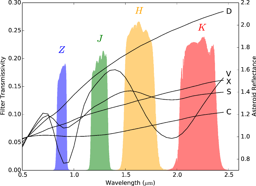
Figure 1: NIR photometric colors are indicative of asteroid compositions. The $Z$, $J$, $H$, and $K$ bandpasses used by UKIRT (Hewett et al., 2006) are plotted together with averaged asteroid reflectance spectra (black lines, DeMeo et al., 2009) of the most common asteroid taxonomic types and complexes (sets of taxonomic types with similar spectral properties.)

2 Observations and Data Analysis

Observations for this project are performed with the Wide Field Camera for UKIRT (WFCAM, Casali et al., 2007). The United Kingdom Infrared Telescope (UKIRT), which is now operated by the University of Hawaii, the University of Arizona, and the Lockheed Martin Advanced Technology Center, is a 3.8 m Cassegrain-type telescope located on Maunakea, Hawai’i. WFCAM consists of four 2k$\times$2k detectors, each of which covers a field of the sky with an edge length of 13.7′. The WFCAM photometric system (Hewett et al., 2006) is mostly identical to the wide-spread Mauna Kea Observatory $J$, $H$, and $K$ near-infrared filters and includes a $Z$ band filter that is very similar to the SDSS $z$ band filter. All these filters have been used in the UKIRT Infrared Deep Sky Survey (UKIDSS, Lawrence et al., 2007). UKIRT is operated in queue mode, allowing for flexibility in the scheduling of observations. We started observations for this project in semester 2014A and obtained 110 observations of 104 different NEOs in semesters 2014A and 2014B. Observations are still ongoing as of writing this.

2.1 Observation Planning

In this program, we acquire observations in the $Z$, $J$, $H$, and $K$ bands. $H$ is the only filter that has not been used for all targets; we added $H$ later to compensate for a potential loss of $Z$ data due to calibration issues. Figure 1 shows that these filter bands sample the spectral slope and silicate band features of the most common asteroid taxonomies well. Our approach is to measure the brightness of our target NEOs in these bands and then compare the differential colors (e.g., $Z-J$, $J-K$) to color data synthesized from measured asteroid spectra (Section 3). Our rapid response approach is key to the success of our program. Most NEOs are discovered when they are brightest, i.e., closest to the observer. After their discovery, NEOs fade quickly at a rate of typically 0.5 mag within one week and 5 mag within 6 weeks as they increase their distance from the observer (Galache et al., 2015). By triggering rapid response spectrophotometric observations of NEOs within a few days of discovery, we are able to observe and characterize objects with absolute magnitudes $H\sim 28$, i.e., with diameters of a few meters. Such rapid response is generally not feasible through classical observing proposals to heavily oversubscribed major research facilities.

Potential targets are identified and uploaded into the UKIRT queue on a daily basis. Accessible targets are identified among those NEOs that have been discovered within the last 4 weeks; this duration is somewhat arbitrary, but usually leads to a number of well-observable and bright potential targets. Since most targets fade quickly in brightness, those that get observed were discovered only a few days before their observation. In the case of the unavailability of rapid-response targets, we upload other accessible NEOs into the queue, which we refer to as “substitute” targets. A target is considered accessible if it has a visible brightness $V\leq 22$, and an airmass $\leq$ 2.0, as provided by the JPL Horizons system (Giorgini et al., 1996), for at least the duration of the estimated integration time from Maunakea. Potential targets are manually selected from the list of accessible targets, prioritizing objects with high absolute magnitudes $H_{V}$ (small sizes) and large values of $H_{V}-V$, where $V$ is the apparent magnitude of the target in the coming night. High values of $H_{V}-V$ ensure that our targets are observed when they are close to the Earth. UKIRT queue observing scripts are automatically created for the selected targets, using the latest orbital elements of the targets as provided by JPL Horizons. The telescope tracks the motion of the target, leading to a trailing of the background sources. We use a frame time of 5 s in each band to minimize the trailing; most targets move at ${\leq}5$ arcsec per minute. The total integration time in each band is a function of the predicted target brightness $V$, typically varying between 30 min and 2 hr in all bands. In our observations, we place the target in the center of WFCAM camera 3, which provides the best noise properties. Different combinations of dither patterns (3.2″ step size) and additional telescope offsets are used to enable the creation of proper flatfield images from the imaging data that are used to mitigate against pixel-to-pixel variability in the detector. In order to account for rotational brightness changes in our targets we intersperse $Z$, $H$, and $K$ observations with $J$ observations, in which the targets are usually bright. A typical filter sequence for a bright target is $JKJZJHJKJ$; fainter targets require longer integration times, involving repetitions of this pattern. Typical frame numbers per filter [$J$, $Z$, $H$, $K$] are [50, 40, 40, 70] for bright targets ($V\leq 19.5$) and [110, 50, 50, 320] for faint targets ($V>20.5$); the integration time is 5 s for each frame. The larger number of frames in $K$ band is a result of the degraded detector sensitivity, the higher background, and reduced solar emission in this band.

2.2 Data Analysis

Basic data reduction is performed by the Cambridge Astronomical Survey Unit (CASU) using the default UKIRT data reduction recipes (Irwin et al., submitted). Reduced individual frames are downloaded from CASU, registered based on 2MASS (Skrutksie et al., 2006) catalog stars in the field, and combined in the frame of the sky (“skycoadd” frame) and in the moving frame of the target (“comove” frame) using SOURCE EXTRACTOR, SCAMP, and SWARP (Bertin and Arnouts, 1996; Bertin et al., 2002; Bertin, 2006). Individual frames are combined in groups of observations in the same band that were taken consecutively (one member of the filter sequence), retaining the filter sequence and providing a skycoadd and comove frame for each filter sequence member. All comove images are inspected to make sure that the target is not contaminated from background sources; if necessary, individual contaminated frames are excluded from the combination process to mitigate against contamination. Aperture photometry is obtained using SOURCE EXTRACTOR. The optimum aperture size is derived from the comove and skycoadd images of each filter sequence member using a curve-of-growth method (Howell, 2006). A common aperture radius is used for all observations of one target that is based on the fraction of flux enclosed for the target and background sources, as well as the resulting signal-to-noise ratios. In the rare case of strongly trailed background sources, we manually select a larger aperture radius to assure that similar flux ratios for both the target and the background sources are enclosed. The magnitude zeropoint of each filter sequence member is derived from the skycoadd image, using an uncertainty-weighted $\chi^{2}$-minimization based on available 2MASS field stars. Typical zeropoint uncertainties are of the order of 0.01 mag or less, using catalog magnitudes from ${\sim}$100 2MASS stars converted into the UKIRT photometric system (Hodgkin et al., 2009).

In order to check the consistency of our photometric calibration, we compare magnitudes measured with our pipeline with standard star magnitudes from the literature for select fields. We obtain reduced image data of 5 standard star fields (Leggett et al., 2006) from the WFCAM Science Archive in the $J$, $H$, and $K$ bands and process them using our default analysis pipeline. We find average magnitude offsets between our 2MASS-calibrated measurements and the literature magnitudes of the order of 0.03 mag, which is smaller than the typical photometric uncertainties observed in our targets.

$Z$ band calibration requires additional treatment, as it is subject to non-negligible reddening effects due to galactic extinction. The transformation from 2MASS $J$, $H$, and $Ks$ (a short-bandpass version of the common $K$ band filter), all of which are barely impacted by reddening, into the UKIRT $Z$ band, which is subject to reddening, requires an offset that was derived within this work. We compare Sloan Digital Sky Survey (SDSS, data release 9) $z$ band magnitudes with $Z$ band magnitudes transformed from 2MASS into UKIRT magnitudes for different fields in the sky as a function of galactic latitude and longitude. We find the offset between both catalogs to be stable at (0.064$\pm$0.035) mag with respect to galactic longitude and latitudes $|b|>15$°, but highly variable for $|b|<15$°. Where available, we hence obtain our $Z$ band calibration from SDSS $z$ band data, which accounts for reddening. Alternatively, we convert 2MASS data into $Z$ band using the transformation given by Hodgkin et al. (2009) and add the offset derived above. We consider $Z$ band calibrations based on 2MASS data at $|b|<15$° unreliable and flag targets accordingly (see Section 5).

From the 110 observations of 104 different NEOs we obtained in 2014A/B, we had to reject 18 observations mostly because they were too faint and the chosen exposure time was too short or the background was too crowded. We adjusted the total integration time for subsequent observations so that our final sample includes 92 useful observations of 86 NEOs.

2.3 Lightcurve Variability Correction and Color Measurement

Irregularly shaped NEOs exhibit potentially significant brightness variations as a function of time. In order to account for the asteroids’ lightcurves, we intersperse our observations in the different filter bands with $J$ band observations. Most targets exhibit a clear variability in the $J$ band. Note that this variability is not caused by transparency variations, which are accounted for through the absolute photometric calibration of our target fields. Aiming for an accurate measurement of the target’s color, we have to account for the target’s brightness variability that is inherent to our brightness measurements. We base this correction on the interspersed $J$ band observations. For each [$H$, $K$, $Z$] band observation, we derive the lightcurve-corrected $J$ band magnitude at the time of the observation through linear interpolation based on those $J$ band observations that are closest in time before and after the non-$J$ band observation. By interpolating the $J$ band brightness at the times of non-$J$ observations, we obtain an approximate measure for the brightness in $J$ at these time. Based on the interpolated $J$ band magnitude, we derive the corresponding colors $J-$[$H$, $K$, $Z$] (see Figure 2). Using the interpolated $J$ band brightness, we can derive the target’s color more accurately than by simply subtracting $J$ from non-$J$ measurements. The uncertainty of each color measurement is defined as the quadratic sum of the uncertainties of all three observations (2$\times J$ plus one non-$J$ band magnitude uncertainty), which results from Gaussian error propagation. If more than one observation is available in either non-$J$ band, the corresponding color is derived as the weighted mean over all measurements of that color, where the weight is the inverse squared color uncertainty. The total color uncertainty is the quadratic sum of the root-sum-square of the involved magnitude uncertainties and the standard deviation of the mean of the individual color determinations, if several measurements are available. From the measured colors we subtract the colors of the Sun, which we obtained with the synthesis method introduced in Section 3.

As a by-product, our method also allows for a qualitative description of the target’s lightcurve. Although our observations usually only cover a fraction of the rotational period of each target, we are able to put constraints on both the target’s brightness variability amplitude ($A^{\star}$) and timescale ($\tau^{\star}$). We define the variability amplitude as the maximum difference in $J$ band magnitudes (also including interpolated $J$ magnitudes from non-$J$ measurements) and the timescale as the difference in time between those measurements. If a lightcurve measurement exhibits more than one maximum and minimum, we measure the amplitude and timescale between two consecutive extrema. The method is graphically presented in Figure 2. Note that $A^{\star}$ and $\tau^{\star}$ should not be mistaken as the target’s rotational amplitude and period. $A^{\star}$ generally provides a lower limit on the lightcurve amplitude of the target as we have to assume that only part of the lightcurve has been sampled; its uncertainty is derived as the quadratic sum of the magnitude uncertainties of the maximum and minimum brightness, providing a measure for the significance of $A^{\star}$. $\tau^{\star}$ only provides a measure for the temporal variability of the brightness of the target; it may suggest a fast or slowly rotating nature of the target.

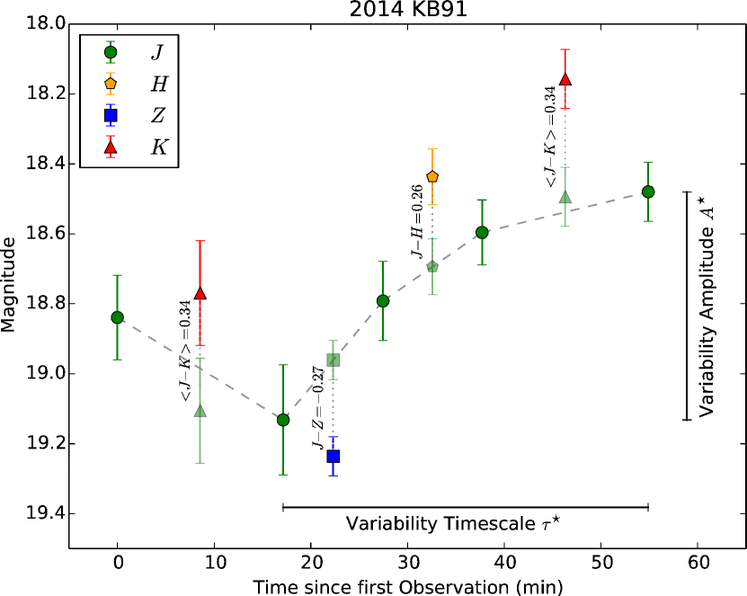
Figure 2: Color determination for NEO 2014 KB91. The target’s lightcurve is clearly visible in the $J$ band observations (green circles). We interpolate between $J$ band observations to obtain the lightcurve-corrected brightness in $J$ at times of non-$J$ observations (dashed line and semi-transparent symbols, see text). Colors are derived by subtracting the non-$J$ magnitudes from these interpolated $J$ magnitudes. The measured colors for 2014 KB91 are $J-H$=-0.05$\pm$0.17, $Z-J$=-0.09$\pm$0.20, $J-K$=-0.02$\pm$0.15, after subtraction of the solar colors. Note that the derived $J-K$ color is a weighted average of two observations; hence, the interpolated $J$ magnitudes for the $K$ band are slightly offset from the linear interpolation, but still agree within 1$\sigma$. We also derive the variability amplitude ($A^{\star}=0.65\pm 0.18$) and the variability timescale ($\tau^{\star}\geq 37.7$ min) from our data (see Section 2.3 for details).

3 Synthesis of NEO NIR Colors from Measured Spectra

In order to interpret our measured asteroid colors, we synthesize asteroid colors from measured asteroid spectra. The largest available database of NEO spectra is the MIT-UH-IRTF Joint Campaign for NEO Spectral Reconnaissance, which obtains NIR spectra of NEOs using SpeX (Rayner et al., 2003) on NASA’s Infrared Telescope Facility. We obtained 614 asteroid spectra from that survey (including a number of duplicate observations) and classified them using the Bus-DeMeo taxonomy spectrum classification on-line routine. We only used spectra that cover the wavelength range from 0.8 to 2.45 $\mu$m and accepted only those classifications from the on-line routine with absolute average residuals of 0.05 or less. We also allowed for multiple classifications if the residuals were within 10% of the minimum residual value. While these restrictions reduce the number of classified spectra (439 spectra), they drastically increase the quality of the synthesized colors. The color-color distribution of different taxonomic types in the Bus-DeMeo System is shown in Figure 3. The plots show that spectroscopic differences between taxonomic complex sub-types and even some independent taxonomic types are subtle. Hence, we decided to distinguish only between a few distinct complexes and types: S-complex (including types S, Sa, Sq, Sqw, Sr, Srw, Sv, and Sw; 171 objects), C-complex and X-complex (including types C, Cb, Cg, Cgh, Ch, X, Xc, Xe, Xk, and Xn; 130 objects), and a small number of independent taxonomic types (D-type and V-type, 18 objects in total). Note that the spectral similarity between C-complex and X-complex asteroids complicates a distinction between members of these complexes. This simplified classification scheme (compared to the full Bus-DeMeo scheme, DeMeo et al., 2009) implies the possibility of mis-classifications due to a lack of less frequent asteroid taxonomic types in our scheme. Figure 3 shows that many less frequent asteroid types fall within the color-space occupied by the main complexes: A, R, O, Q, and L-type asteroids are likely to be mistaken for S-complex asteroids, whereas T and K-type asteroids might be classified as C/X-complex asteroids. This ambiguity within the smaller taxonomic type groups, as well as the ambiguity between the C and X-complexes could only be resolved with a significantly higher precision in the measurement of the asteroid colors.

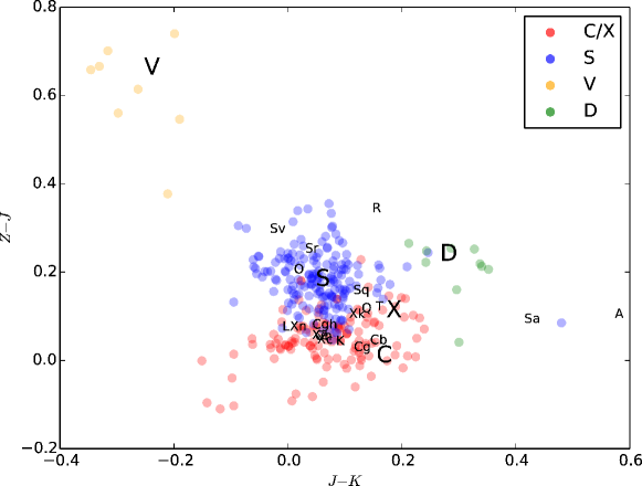
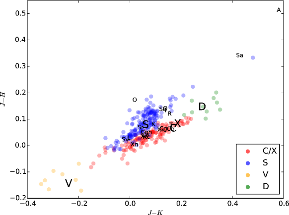
Figure 3: Asteroid color training sample derived from MIT-UH-IRTF data. Letters indicate the average locations of individual taxonomic types; taxonomic complexes and types that can be identified in this work are highlighted (average reflectance spectra from DeMeo et al., 2009).

Each classified spectrum is turned into synthesized colors in the UKIRT photometric bands $Z$, $J$, $H$, and $K$ (bandpass information is provided by Hewett et al., 2006). In order to derive the absolute flux $F_{f,t}$ in a certain bandpass, we convolve the spectral response $R_{f}(\lambda)$ of each filter $f$ with the product of the respective asteroid reflectance spectrum $A_{t}(\lambda)$ of taxonomic type $t$ and a spectrum of the Sun $S(\lambda)$ over the whole bandpass wavelength range:

$$F_{f,t}=\int R_{f}(\lambda)\;A_{t}(\lambda)S(\lambda)\;\lambda\ d\lambda.$$ (1)

From this flux, we derive the resulting synthetic magnitude and calibrate it in the Vega magnitude system. We derive the zeropoint magnitude using Equation 1 by setting $A_{t}(\lambda)\equiv 1$ and replacing $S(\lambda)$ with a spectrum of Vega. Colors are derived from the calibrated magnitudes and solar colors ($J-K=0.354$, $Z-J=0.369$, $J-H=0.304$) are subtracted. Color-color plots are displayed in Figure 3, showing the distribution of synthesized asteroid spectra of different taxonomic types in $Z-J$ vs. $J-K$ and $J-H$ vs. $J-K$ color spaces.

4 Taxonomic Classification

We classify our sample targets based on the sample of synthesized asteroid NIR colors (see Section 3) in a machine-learning approach using the scikit-learn module (Pedregosa et al., 2011) for Python. In order to find the most reliable classification algorithm for our problem, we tested the accuracy of different methods, including different Nearest-Neighbor, Support Vector Machine (SVM), and a Gaussian Naive Bayes method, that are provided within scikit-learn (see http://scikit-learn.org for discussions of the individual methods). In our test, we remove one object at a time from the sample of 319 synthesized asteroid NIR colors of S-complex, C/X-complex, D-type, and V-type asteroids (see Section 3) and predict its class based on the different methods that have been trained on the rest of the sample. Table 1 compares the numbers of correct classifications for the different methods, considering two different cases: the first case assumes two color measurements ($Z-J$ and $J-K$); the second case assumes three color measurements ($Z-J$, $J-H$, and $J-K$). The accuracy of the algorithms varies between the two cases; generally, the 3-color case derives more accurate results based on the fact that the increased number of degrees of freedom puts additional constraints on the classification problem. In the 2-color case, the $k$-Nearest Neighbor ($k=5$) and the Gaussian Naive Bayes methods achieve the same overall accuracy; in the 3-color case, the $k$-Nearest Neighbor ($k=1$) is the most accurate method. Hence, we adopt the $k$-Nearest Neighbor ($k=1$) method if 3 asteroid colors are available and the Gaussian Naive Bayes method if only 2 colors are available. We refrain from using $k$-Nearest Neighbor ($k=5$) as it relies on fairly large training samples for the different taxonomic types, which are not available in the case of V-type and D-type asteroids.

Table 1: Classification Algorithm Accuracy Comparison.

Algorithm	2 Colors	3 Colors
Nearest Centroid	85.6%	89.3%
$k$-Nearest Neighbor ($k$=1)	85.9%	96.2%
$k$-Nearest Neighbor ($k$=3)	87.8%	94.4%
$k$-Nearest Neighbor ($k$=5)	88.4%	95.0%
SVM, linear kernel	85.0%	91.2%
SVM, polynomial kernel (3rd degree)	53.6%	53.6%
SVM, radial basis function kernel	85.0%	91.2%
Gaussian Naive Bayes	88.4%	92.5%

In order to account for uncertainties in the measurement of each target’s color, we use a Monte Carlo approach in which we randomize the measured colors within the corresponding 1$\sigma$ uncertainties in each color based on a Gaussian distribution in $10^{6}$ trials. We classify the whole ensemble using the respective algorithm trained on our set of synthesized asteroid NIR colors and count the frequency of classifications in the individual taxonomic types. Thus, we obtain classification probabilities for the individual taxonomies and we adopt the most likely taxonomic class for the target.

5 Results

Figure 4 shows an example color-color plot that is based on measured $Z-J$ and $J-K$ colors of our sample targets. The probabilistic classification results for all data are presented in Table 2. Some of our sample targets were observed at low galactic latitudes and calibrated using $Z$ band magnitudes that were transformed from 2MASS data, potentially leading to inaccuracies in the $Z$ magnitudes (see Section 2.2). Furthermore, some targets exhibit highly variable lightcurves that make it impossible to put constraints on the variability timescale, or show potential inconsistencies in the measured lightcurve. Both effects can potentially influence the reliability of the color measurements (see Section 6 for a discussion). Taxonomic classifications that are subject to either of the irregularities listed above should be considered with care; affected targets are marked in the Notes column of Table 2.

Only considering classifications with a probability ${\geq}50$%, total root-mean-square color uncertainties ${\leq}0.3$ mag, and observations that are not affected by irregularities as discussed above leads to reliable classifications for 46 observations of 43 different NEOs. 25 more observations are subject to irregularities, 18 observations suffer from a low signal-to-noise ratio (color uncertainties ${>}0.3$ mag), and 7 observations lead to ambiguous taxonomic classifications (probabilities for all taxonomic classifications ${<}50$%). Note that the ratio of reliable classifications is higher for those targets that were observed more recently, which is a result of an increase of integration time in our observation planning.

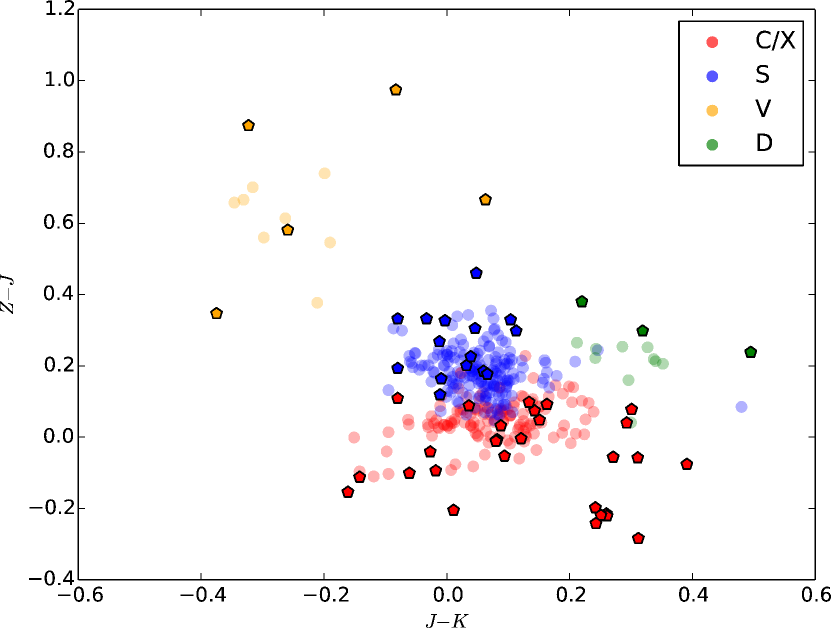
Figure 4: Distribution of observed NEOs in $Z-J$ and $J-K$ color space. Semi-transparent circles represent the training samples shown in Figure 3. The color of each pentagon reflects the most likely taxonomic classification based on the Monte Carlo method described in Section 4 using the measured $Z-J$ and $J-K$ colors only. In this plot, we only show NEOs with a minimum probability of 50% for a taxonomic class, a root-mean-square color uncertainty of less than 0.3 mag, and observations that are not affected by irregularities (51 out of 67 targets with $Z$, $J$, $K$ observations meet these criteria, see Table 2). Solar colors have been subtracted from each datapoint.

Table 2: Observations and Results.

Object	Obs. Midtime	Dur.	$H_{V}$	$V$	$J_{\mathrm{Median}}$	$Z-J$	$J-H$	$J-K$	$A^{\star}$	$\tau^{\star}$	C/X	D	S	V	Notes
	(UT)	(hr)	(mag)	(mag)	(mag)	(mag)	(mag)	(mag)	(mag)	(min)	Prob.	Prob.	Prob.	Prob.
99799⋆	14-03-21 08:51	0.3	18.30	19.89	18.91	0.81$\pm$0.41	$\cdots$	0.21$\pm$0.31	0.40$\pm$0.27	${\geq}$7.0	0.06	0.29	0.08	0.57
125268⋆	15-01-18 06:32	2.0	16.10	20.06	18.59	0.30$\pm$0.11	$\cdots$	0.11$\pm$0.08	0.20$\pm$0.17	40.0	0.05	0.09	0.84	0.01
141857⋆	15-01-17 07:12	2.0	16.30	19.83	18.31	0.52$\pm$0.12	$\cdots$	-0.04$\pm$0.07	0.60$\pm$0.10	36.6	0.00	0.00	0.33	0.67
2004 JN13⋆	15-01-15 07:00	0.6	15.30	16.55	15.12	-0.07$\pm$0.02	$\cdots$	0.11$\pm$0.01	0.05$\pm$0.01	${\geq}$33.6	1.00	0.00	0.00	0.00
2006 WW⋆	15-01-17 14:16	1.9	16.10	19.90	18.67	0.54$\pm$0.10	$\cdots$	0.17$\pm$0.08	0.27$\pm$0.12	${\geq}$44.2	0.00	0.41	0.43	0.16
2009 TG10⋆	14-04-15 11:40	0.2	17.60	16.90	15.28	-0.11$\pm$0.02	$\cdots$	-0.14$\pm$0.04	0.09$\pm$0.05	${\geq}$6.5	1.00	0.00	0.00	0.00
2010 AG79⋆	14-12-29 06:32	1.5	19.90	20.86	19.74	-0.53$\pm$0.27	$\cdots$	0.67$\pm$0.32	0.66$\pm$0.47	22.0	0.97	0.00	0.00	0.03
2011 CH50⋆	14-04-04 05:33	0.2	21.80	18.48	17.48	-0.06$\pm$0.10	$\cdots$	0.31$\pm$0.08	0.17$\pm$0.10	4.0	0.90	0.10	0.00	0.00
2011 CH50⋆	14-04-16 09:57	0.2	21.80	18.16	16.99	-0.00$\pm$0.07	$\cdots$	0.12$\pm$0.10	0.13$\pm$0.16	5.0	0.94	0.01	0.05	0.00
2011 OL5⋆	14-12-29 15:35	0.6	20.20	19.28	18.50	0.18$\pm$0.13	$\cdots$	0.09$\pm$0.19	0.36$\pm$0.29	19.5	0.30	0.19	0.47	0.04
2011 WK15⋆	14-12-29 14:58	0.6	19.70	18.29	16.90	0.05$\pm$0.04	$\cdots$	0.15$\pm$0.04	0.08$\pm$0.03	${\geq}$33.8	0.96	0.00	0.04	0.00
2012 CO46⋆	14-12-29 11:53	1.4	22.80	20.26	19.41	-0.06$\pm$0.25	$\cdots$	0.27$\pm$0.18	0.52$\pm$0.27	${\geq}$44.2	0.73	0.17	0.09	0.00
2013 BM76⋆	15-01-17 15:49	0.9	20.20	19.76	18.80	0.04$\pm$0.14	$\cdots$	0.29$\pm$0.11	0.10$\pm$0.16	${\geq}$42.4	0.63	0.30	0.07	0.00
2013 BM76⋆	15-01-20 15:31	0.9	20.20	19.74	18.76	0.33$\pm$0.12	$\cdots$	0.10$\pm$0.09	0.19$\pm$0.09	${\geq}$23.1	0.04	0.10	0.83	0.03
2014 GF1	14-04-09 10:39	1.1	26.00	21.21	19.85	0.24$\pm$0.25	$\cdots$	0.49$\pm$0.18	0.11$\pm$0.22	${\geq}$37.4	0.38	0.58	0.03	0.01
2014 GH17	14-04-09 09:08	1.3	21.90	20.33	19.47	0.30$\pm$0.25	$\cdots$	0.32$\pm$0.23	0.17$\pm$0.22	12.9	0.25	0.50	0.19	0.06
2014 GV48	14-04-13 08:25	1.1	25.80	20.18	19.15	0.28$\pm$0.27	$\cdots$	0.04$\pm$0.16	0.59$\pm$0.22	${\geq}$29.5	0.27	0.11	0.41	0.21
2014 HE3	14-10-12 10:23	0.5	19.90	19.09	18.07	-0.27$\pm$0.13	0.24$\pm$0.16	0.13$\pm$0.15	0.34$\pm$0.14	10.4	0.73	0.04	0.23	0.00
2014 HW	14-04-24 11:50	2.2	28.40	18.94	17.67	0.33$\pm$0.11	$\cdots$	0.06$\pm$0.08	0.40$\pm$0.20	12.0	0.02	0.02	0.91	0.04
2014 JA31	14-05-12 13:51	0.4	23.60	19.18	18.21	-0.04$\pm$0.17	$\cdots$	-0.03$\pm$0.20	0.30$\pm$0.18	${\geq}$	0.82	0.02	0.12	0.03
2014 JG78	14-05-21 12:15	0.8	19.60	20.44	19.75	-0.17$\pm$0.31	$\cdots$	0.27$\pm$0.32	0.70$\pm$0.57	${\geq}$25.3	0.80	0.10	0.06	0.05
2014 JR25	14-05-11 15:00	0.4	23.40	18.39	17.20	-0.20$\pm$0.09	$\cdots$	0.01$\pm$0.09	0.20$\pm$0.07	${\geq}$12.3	1.00	0.00	0.00	0.00
2014 JS57	14-05-18 13:51	0.8	22.20	20.42	18.84	-0.06$\pm$0.16	$\cdots$	0.07$\pm$0.23	0.55$\pm$0.38	${\geq}$25.0	0.85	0.05	0.09	0.02
2014 JT54	14-05-12 08:45	0.9	24.10	20.19	18.82	0.26$\pm$0.21	$\cdots$	-0.08$\pm$0.18	0.56$\pm$0.23	${\geq}$35.6	0.26	0.04	0.40	0.30
2014 JV54	14-05-20 14:01	0.4	25.90	20.33	19.16	0.14$\pm$0.30	$\cdots$	-0.08$\pm$0.27	0.56$\pm$0.28	${\geq}$22.0	0.45	0.07	0.21	0.26
2014 JW24	14-05-11 06:36	0.4	23.90	19.77	18.60	0.22$\pm$0.26	$\cdots$	-0.10$\pm$0.20	0.46$\pm$0.25	${\geq}$21.8	0.35	0.04	0.30	0.31
2014 JY30	14-05-11 07:01	0.4	25.40	20.12	19.09	0.32$\pm$0.41	$\cdots$	-0.49$\pm$0.32	0.59$\pm$0.38	3.2	0.23	0.01	0.05	0.71
2014 KA46	14-06-08 10:19	0.9	24.40	20.09	18.58	0.28$\pm$0.21	-0.36$\pm$0.18	0.08$\pm$0.25	0.94$\pm$0.23	${\geq}$17.4	0.40	0.10	0.13	0.37
2014 KB91	14-06-04 11:10	0.9	20.20	19.88	18.79	-0.09$\pm$0.20	-0.05$\pm$0.17	-0.02$\pm$0.15	0.65$\pm$0.18	${\geq}$37.7	0.83	0.01	0.15	0.02
2014 KD	14-05-20 13:36	0.4	24.40	18.95	16.63	0.21$\pm$0.08	$\cdots$	0.17$\pm$0.10	0.53$\pm$0.12	9.0	0.11	0.28	0.61	0.00
2014 KO62	14-06-03 12:07	1.0	26.20	20.29	18.97	0.38$\pm$0.15	-0.18$\pm$0.22	0.22$\pm$0.18	0.97$\pm$0.19	30.0	0.15	0.29	0.38	0.18
2014 KX86	14-06-03 11:02	0.9	26.50	21.03	19.37	0.87$\pm$0.22	$\cdots$	-0.32$\pm$0.33	1.16$\pm$0.36	${\geq}$27.6	0.00	0.03	0.01	0.96
2014 MC6	14-10-11 11:10	1.0	19.40	19.62	18.74	-0.08$\pm$0.18	0.10$\pm$0.17	0.39$\pm$0.16	0.39$\pm$0.18	${\geq}$27.8	0.34	0.40	0.26	0.00
2014 ME18	14-07-26 08:03	1.4	23.00	21.08	19.85	0.15$\pm$0.26	0.31$\pm$0.29	0.08$\pm$0.27	0.80$\pm$0.46	24.4	0.17	0.10	0.68	0.04
2014 MJ27	14-07-26 09:42	1.5	23.10	20.91	19.89	0.08$\pm$0.33	-0.22$\pm$0.38	0.30$\pm$0.26	0.92$\pm$0.58	17.9	0.47	0.24	0.19	0.09
2014 MK55	14-12-30 09:50	1.1	21.40	20.40	19.39	0.36$\pm$0.23	$\cdots$	0.11$\pm$0.36	0.47$\pm$0.57	32.8	0.17	0.30	0.24	0.29
2014 MK6	14-07-25 07:47	1.0	21.00	19.61	18.87	-0.21$\pm$0.26	0.47$\pm$0.27	0.26$\pm$0.22	0.40$\pm$0.34	${\geq}$17.4	0.25	0.06	0.69	0.00
2014 MM55	14-10-13 13:24	0.5	18.70	18.79	17.78	-0.22$\pm$0.11	0.07$\pm$0.11	0.26$\pm$0.08	0.42$\pm$0.09	${\geq}$29.6	0.91	0.08	0.01	0.00
2014 MP41	14-07-12 13:50	0.9	18.40	19.73	19.61	-0.16$\pm$0.33	0.16$\pm$0.32	-0.04$\pm$0.27	0.57$\pm$0.27	${\geq}$38.7	0.59	0.04	0.34	0.04
2014 MQ60	14-07-25 09:51	1.3	22.40	20.44	19.22	0.58$\pm$0.26	0.18$\pm$0.31	-0.26$\pm$0.28	0.85$\pm$0.32	12.0	0.03	0.01	0.32	0.64
2014 MX	14-07-25 11:38	1.4	24.10	20.84	19.78	-0.20$\pm$0.25	-0.27$\pm$0.69	0.24$\pm$0.29	1.71$\pm$0.76	16.1	0.67	0.08	0.22	0.03
2014 MX17	14-07-11 11:14	0.9	20.50	19.62	18.38	0.11$\pm$0.10	0.07$\pm$0.10	0.04$\pm$0.09	0.16$\pm$0.09	${\geq}$18.0	0.41	0.01	0.58	0.00
2014 NB52	14-07-11 13:09	1.4	21.70	20.18	19.32	-0.15$\pm$0.27	0.38$\pm$0.26	0.34$\pm$0.18	0.69$\pm$0.26	${\geq}$33.3	0.25	0.13	0.62	0.00
2014 NC39	14-07-16 09:58	0.9	21.70	20.54	19.85	-0.18$\pm$0.37	$\cdots$	0.57$\pm$0.30	0.55$\pm$0.43	${\geq}$55.1	0.84	0.12	0.02	0.02
2014 ND52	14-07-12 12:22	1.4	23.70	20.33	19.24	0.29$\pm$0.19	-0.04$\pm$0.23	0.14$\pm$0.17	0.50$\pm$0.23	${\geq}$33.7	0.24	0.19	0.46	0.11
2014 NE3	14-07-11 12:04	0.5	20.10	18.58	17.49	-0.01$\pm$0.09	0.12$\pm$0.09	0.08$\pm$0.07	0.28$\pm$0.09	${\geq}$	0.56	0.01	0.43	0.00
2014 NE39	14-07-18 10:47	0.9	20.60	20.15	18.99	-0.05$\pm$0.16	0.17$\pm$0.17	0.09$\pm$0.16	0.31$\pm$0.16	${\geq}$19.0	0.50	0.08	0.43	0.00
2014 NG3	14-07-10 14:26	0.9	24.20	20.06	19.02	-0.28$\pm$0.18	0.54$\pm$0.19	0.31$\pm$0.13	0.41$\pm$0.17	10.3	0.17	0.03	0.79	0.00
2014 NL52	14-07-15 11:58	1.4	23.60	20.34	19.63	$\cdots$	0.23$\pm$0.21	0.37$\pm$0.23	0.61$\pm$0.29	25.2	0.25	0.30	0.45	0.00
2014 OG1	14-07-25 08:37	0.5	21.60	18.48	17.57	-0.22$\pm$0.17	0.06$\pm$0.14	0.25$\pm$0.13	0.57$\pm$0.15	${\geq}$	0.81	0.14	0.06	0.00
2014 OT111	14-07-31 09:44	0.5	21.70	17.39	15.92	0.07$\pm$0.03	0.11$\pm$0.03	0.14$\pm$0.02	0.10$\pm$0.02	${\geq}$14.4	0.60	0.00	0.40	0.00
2014 OV3	14-07-29 09:26	0.9	23.20	19.43	17.88	0.67$\pm$0.09	-0.07$\pm$0.09	0.06$\pm$0.08	0.43$\pm$0.09	${\geq}$27.5	0.00	0.00	0.25	0.75
2014 OV3	15-01-18 13:14	1.4	23.20	20.41	19.18	0.20$\pm$0.20	$\cdots$	0.18$\pm$0.18	0.60$\pm$0.18	${\geq}$79.0	0.31	0.31	0.34	0.04
2014 PL51	14-10-11 10:10	0.5	20.40	18.84	17.61	0.10$\pm$0.11	0.20$\pm$0.12	-0.01$\pm$0.12	0.30$\pm$0.12	${\geq}$19.6	0.15	0.01	0.83	0.00
2014 RC12	14-10-12 15:19	1.0	18.80	19.86	18.48	0.06$\pm$0.14	0.32$\pm$0.14	-0.10$\pm$0.11	0.58$\pm$0.13	${\geq}$30.0	0.11	0.00	0.89	0.00
2014 RL12	15-01-18 11:26	1.9	17.90	17.93	16.66	0.23$\pm$0.03	$\cdots$	0.03$\pm$0.05	0.19$\pm$0.08	89.3	0.00	0.00	1.00	0.00
2014 RL12	15-01-19 07:38	2.1	17.90	18.00	16.61	0.16$\pm$0.03	$\cdots$	-0.07$\pm$0.02	0.11$\pm$0.03	${\geq}$99.3	0.02	0.00	0.98	0.00
2014 RQ17	14-12-29 13:36	1.9	22.30	20.70	19.47	0.77$\pm$0.22	$\cdots$	0.05$\pm$0.19	0.52$\pm$0.29	11.4	0.00	0.14	0.09	0.77
2014 SF145	14-12-29 10:47	0.6	22.60	19.31	18.10	0.12$\pm$0.11	$\cdots$	0.15$\pm$0.10	0.17$\pm$0.14	12.2	0.48	0.13	0.38	0.00
2014 SM143	14-10-12 14:30	0.5	20.30	17.15	15.97	0.09$\pm$0.03	0.21$\pm$0.03	0.16$\pm$0.02	0.06$\pm$0.03	${\geq}$28.9	0.02	0.00	0.98	0.00
2014 SM261	14-10-12 11:16	0.5	21.10	19.05	17.87	0.10$\pm$0.13	0.22$\pm$0.14	0.31$\pm$0.11	0.19$\pm$0.14	${\geq}$14.3	0.13	0.43	0.44	0.00
2014 SS1	14-10-12 09:36	0.5	21.70	18.75	17.49	0.18$\pm$0.10	0.14$\pm$0.10	0.06$\pm$0.08	0.30$\pm$0.09	${\geq}$10.0	0.14	0.02	0.84	0.00
2014 SZ264	14-10-11 12:10	0.9	18.60	19.98	18.68	0.10$\pm$0.14	0.29$\pm$0.16	0.34$\pm$0.13	0.13$\pm$0.15	20.7	0.08	0.32	0.60	0.00
2014 TJ17	14-10-11 08:58	0.5	24.90	18.70	17.64	0.33$\pm$0.14	0.06$\pm$0.14	-0.00$\pm$0.15	0.40$\pm$0.13	${\geq}$7.0	0.09	0.05	0.75	0.11
2014 TN17	14-10-10 07:12	0.5	21.50	19.07	17.72	0.24$\pm$0.14	-0.10$\pm$0.13	-0.00$\pm$0.24	0.55$\pm$0.26	9.9	0.31	0.12	0.36	0.21
2014 TV	14-10-11 09:36	0.5	24.40	18.91	18.04	-0.24$\pm$0.26	0.61$\pm$0.24	0.24$\pm$0.16	0.82$\pm$0.25	${\geq}$14.8	0.16	0.02	0.82	0.00
2014 TZ17	14-10-16 14:40	0.9	22.70	19.62	18.21	0.12$\pm$0.09	0.08$\pm$0.09	-0.01$\pm$0.09	0.22$\pm$0.08	${\geq}$38.1	0.29	0.00	0.71	0.00
2014 UA176	14-11-05 11:19	0.6	26.70	18.94	17.69	0.30$\pm$0.10	$\cdots$	0.05$\pm$0.08	0.16$\pm$0.12	${\geq}$26.4	0.03	0.02	0.92	0.03
2014 UF206	15-01-15 07:51	0.8	18.80	15.41	13.90	-0.01$\pm$0.01	$\cdots$	0.08$\pm$0.01	0.10$\pm$0.01	${\geq}$33.8	1.00	0.00	0.00	0.00
2014 US	14-11-05 10:38	0.6	19.10	18.14	16.84	0.11$\pm$0.05	$\cdots$	-0.08$\pm$0.03	0.04$\pm$0.03	${\geq}$14.9	0.54	0.00	0.46	0.00
2014 UT33	14-11-04 14:10	0.6	23.40	18.37	17.10	-0.25$\pm$0.06	$\cdots$	0.01$\pm$0.05	0.05$\pm$0.05	${\geq}$14.3	1.00	0.00	0.00	0.00
2014 UV115	14-11-05 14:11	0.6	22.70	19.17	17.50	0.21$\pm$0.06	$\cdots$	0.20$\pm$0.04	0.15$\pm$0.05	5.1	0.10	0.27	0.63	0.00
2014 UV210	15-01-17 12:15	1.9	26.90	20.65	19.65	-0.25$\pm$0.30	$\cdots$	0.25$\pm$0.31	1.00$\pm$0.31	23.1	0.85	0.06	0.04	0.05
2014 VM	14-11-10 11:51	0.6	17.70	17.97	16.66	0.33$\pm$0.04	$\cdots$	-0.08$\pm$0.06	0.09$\pm$0.03	${\geq}$19.5	0.00	0.00	0.89	0.11
2014 VP	14-11-08 11:34	0.9	22.80	19.51	18.23	0.03$\pm$0.12	$\cdots$	-0.21$\pm$0.11	0.16$\pm$0.10	${\geq}$22.9	0.79	0.00	0.12	0.09
2014 WJ201	14-12-07 12:06	0.9	24.80	19.84	19.28	0.35$\pm$0.27	$\cdots$	-0.38$\pm$0.25	0.23$\pm$0.22	7.9	0.16	0.01	0.10	0.73
2014 WJ70	15-01-16 14:10	1.4	17.70	19.25	18.05	0.10$\pm$0.08	$\cdots$	0.13$\pm$0.06	0.18$\pm$0.07	${\geq}$23.0	0.59	0.02	0.39	0.00
2014 WP4	14-12-02 12:24	1.1	24.30	20.01	18.55	0.97$\pm$0.15	$\cdots$	-0.08$\pm$0.09	0.16$\pm$0.10	${\geq}$38.7	0.00	0.00	0.00	1.00
2014 XJ3	14-12-15 10:09	0.6	20.10	17.16	15.70	0.27$\pm$0.03	$\cdots$	-0.01$\pm$0.03	0.07$\pm$0.02	${\geq}$19.9	0.00	0.00	1.00	0.00
2014 YD	15-01-15 13:13	1.4	24.30	20.14	18.78	0.16$\pm$0.18	$\cdots$	-0.01$\pm$0.12	0.40$\pm$0.15	22.0	0.39	0.02	0.51	0.07
2014 YE35	15-01-13 09:25	0.6	20.30	18.49	17.11	0.46$\pm$0.06	$\cdots$	0.05$\pm$0.06	0.10$\pm$0.05	${\geq}$19.4	0.00	0.00	0.88	0.12
2014 YU41	15-01-14 13:14	2.0	23.80	21.00	19.94	-0.02$\pm$0.26	$\cdots$	0.23$\pm$0.19	0.56$\pm$0.41	${\geq}$62.1	0.68	0.18	0.13	0.01
2014 YV34	15-01-13 08:42	0.6	19.50	18.55	17.26	0.23$\pm$0.06	$\cdots$	0.04$\pm$0.04	0.07$\pm$0.05	${\geq}$14.4	0.02	0.00	0.98	0.00
2014 YW34	15-01-16 11:07	1.4	21.60	20.46	19.27	0.18$\pm$0.21	$\cdots$	0.07$\pm$0.12	0.48$\pm$0.17	22.8	0.38	0.07	0.50	0.05
2014 YY43	15-01-18 14:29	0.9	19.40	19.71	18.77	0.19$\pm$0.14	$\cdots$	-0.08$\pm$0.10	0.32$\pm$0.11	7.9	0.30	0.00	0.58	0.11
2015 AN44	15-01-20 10:34	1.4	25.20	20.38	19.17	0.20$\pm$0.14	$\cdots$	0.03$\pm$0.12	0.57$\pm$0.15	${\geq}$33.2	0.27	0.04	0.65	0.04
2015 AP44	15-01-20 12:23	1.9	26.20	20.45	19.54	0.03$\pm$0.20	$\cdots$	0.09$\pm$0.12	0.48$\pm$0.19	${\geq}$88.7	0.65	0.05	0.28	0.01
2015 AR45	15-01-20 09:27	0.6	19.80	19.32	18.12	0.33$\pm$0.11	$\cdots$	-0.03$\pm$0.14	0.29$\pm$0.22	19.3	0.03	0.04	0.70	0.23
2015 BD	15-01-20 13:51	0.6	23.90	19.51	18.44	0.15$\pm$0.12	$\cdots$	0.23$\pm$0.14	0.51$\pm$0.08	${\geq}$19.6	0.35	0.36	0.29	0.00
2015 BG92	15-01-24 12:16	0.4	25.10	19.08	17.80	0.09$\pm$0.10	$\cdots$	0.04$\pm$0.10	0.11$\pm$0.08	${\geq}$14.5	0.59	0.01	0.39	0.00
2015 BG92	15-01-25 09:50	0.4	25.10	18.92	17.52	-0.15$\pm$0.10	$\cdots$	-0.16$\pm$0.10	0.32$\pm$0.09	${\geq}$19.8	1.00	0.00	0.00	0.00
2015 BG92	15-01-26 09:59	0.6	25.10	18.75	17.46	-0.10$\pm$0.06	$\cdots$	-0.06$\pm$0.05	0.23$\pm$0.05	${\geq}$14.4	1.00	0.00	0.00	0.00

Note. — The table lists for each target its official number or designation, observation midtime of the entire filter sequence, the observation duration, the absolute ($H_{V}$) and apparent visible ($V$) magnitude as provided by JPL Horizons at the time of the observation, the median $J$ band brightness from all our measurements, the measured color indices (from which solar colors have been subtracted), the variability amplitude ($A^{\star}$) and timescale ($\tau^{\star}$), and the classification probabilities for the individual taxonomic complexes and types. For each target we use all available colors ($Z-J$, $J-K$, and $J-H$, where available) to provide the best-possible accuracy in our taxonomic classification; bold numbers highlight reliable classifications with a probability ${\geq}50$% and total root-mean-square color uncertainties ${\leq}0.3$ mag. Note that faint targets usually have high uncertainties in their color measurements, leading to a less reliable classification result.

6 Discussion

We investigate the consistency of our color measurements and classifications based on three targets with two or more observations that do not suffer from irregularities (notes in Table 2): 2011 CH50, 2013 BM76, and 2015 BG92. These targets were observed twice or more as a result of an aborted observation due to rapidly changing weather conditions and hence have shorter than intended integration times. Duplicate observations were also obtained in a few cases by the UKIRT telescope operators to test telescope operations. We find multiple color measurements and variability amplitudes of all objects to agree within 1–2$\sigma$. In Table 2, we marked sample targets that show suspicious lightcurve behavior in the form of lightcurve inconsistencies (marked with “2” in the Notes column) or a highly variable lightcurve (marked with “3” in the Notes column). Nevertheless, we believe that our linear-interpolation approach provides the most robust results in the majority of cases. Non-linear interpolation, e.g., using third-order polynomials or splines, would require additional lightcurve information that is currently not available for our sample targets. In a few cases, discrepancies in $Z-J$ color measurement might also be caused by the lack of extinction correction in the transformation of 2MASS data into $Z$ band data (see Section 2.2; targets that are potentially affected by this effect are marked with “1” in the Notes columns of Table 2).

We compare our results to optical spectra obtained within the MANOS project (MANOS classifications taken from Hinkle, 2016); we could not find spectral data of our sample targets in the further literature. We find an overlap of 2 targets with MANOS: 2014 HW (MANOS: S-type, this work: 91% S-complex probability) and 2014 UV210 (MANOS: Cb/Cgh-type, this work: 85% C-complex probability). Note that both targets suffer from irregularities (notes in Table 2) and we are still able to reproduce the MANOS results with a high level of confidence. Five of our sample targets have measured lightcurves, which allows us to compare our variability amplitude ($A^{\star}$) and timescale ($\tau^{\star}$) to the measured rotational amplitude and period. Warner (2015b) finds a period of 31.3 min and an amplitude of 0.99 mag for 2014 RQ17, for which we find $\tau^{\star}=11.4$ min and $A^{\star}=0.52\pm 0.29$ mag. For 2014 SS1, Warner (2015a) finds a period of 16.63 hr and an amplitude of 0.43 mag; we find $\tau^{\star}\geq 10$ min and $A^{\star}=0.30\pm 0.09$ mag. Additional information is available from the MANOS project for 2014 HW (3.8 min, 1.07 mag, our results: $\tau^{\star}=12$ min, $A^{\star}=0.4\pm 0.2$ mag), 2014 UV210 (33.4 min, 0.91 mag, our results: $\tau^{\star}=23.1$ min, $A^{\star}=1.00\pm 0.31$ mag), 2015 BG92 (10.7 min, 0.36 mag, our results: $\tau^{\star}\geq 14.4$ min, $A^{\star}\geq 0.11$ mag). For three out of five targets with lightcurve data we find $\tau^{\star}$ to be smaller than the rotational period, which is a result of the fact that $\tau^{\star}$ only provides a sense of the timescale on which the lightcurve changes. In those two cases in which $\tau^{\star}$ is greater than the rotational period, we account this to the fact that our sampling frequency is too coarse to properly resolve the target’s lightcurve. $A^{\star}$ is smaller than the lightcurve amplitude in all cases and agrees with the actual amplitude within 3$\sigma$ in 3 cases. This behavior is expected since we usually cover only part of the target rotation with our UKIRT observations. Based on this assessment, we believe that $A^{\star}$ and $\tau^{\star}$ are useful parameters that provide some constraints on the target’s lightcurve behavior.

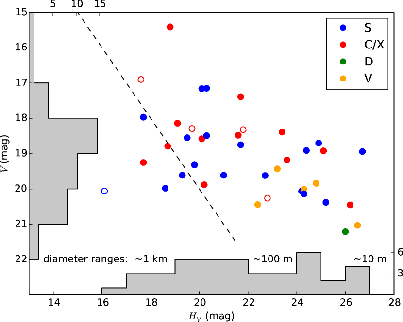
Figure 5: Distribution of sample targets as a function of their absolute magnitude $H_{V}$ and their apparent magnitude $V$ at the time of observation; $V$ magnitudes are predicted magnitudes from the JPL Horizons system. We only show those targets with reliable taxonomic classifications, i.e., with taxonomy probability ${\geq}50$% and root-mean-square color uncertainties ${\leq}0.3$ mag. Filled circles represent targets that were observed within 4 weeks of discovery; open circles are substitute targets that were observed due to the unavailability of rapid response targets. The bottom of the plot shows a histogram of the $H_{V}$ magnitude distribution of our targets, the majority of which have diameters smaller than 1 km; the vertical axis shows a histogram of the $V$ magnitudes. The dashed line represents $V=H_{V}$; most of our targets have been observed when $V<H_{V}$. We are able to derive reliable taxonomic classifications for targets with $V<21$ mag.

We qualitatively investigate the performance of our rapid-response observing approach. Figure 5 shows the distribution of our sample targets as a function of their absolute magnitude $H_{V}$ and their apparent magnitude $V$ at the time of observation. We only show those targets for which we could obtain reliable taxonomic classifications and for which the observations do not suffer from irregularities (notes in Table 2). 90% of our reliable sample targets have $H_{V}>18$ mag, corresponding to asteroid diameters ${\lesssim}1$ km; 38% are smaller than ${\sim}100$ m ($H_{V}\geq 23$ mag). Most of our rapid-response targets (excluding substitute targets) have been observed at $V<H_{V}$, which indicates an efficient way to study small asteroids. Our smallest target, 2014 HW, has $H_{V}$=28.4 mag, but we observed it at V=18.9 mag ($H_{V}-V\sim 9.5$) as a result of our rapid-response observing approach. 2014 HW is not shown on Figure 5, as it is affected by lightcurve inconsistencies. This target most likely has a diameter of only a few meters (based on albedo estimates for S-type asteroids from Thomas et al., 2011), and our comparison to MANOS data (above) confirms that we can derive a reliable classification for such small targets. Figure 5 shows that we are able to obtain reliable data for NEOs with $V\leq 21$ mag, which is fainter than targets accessible to spectroscopic observations, except for those done with the largest telescopes.

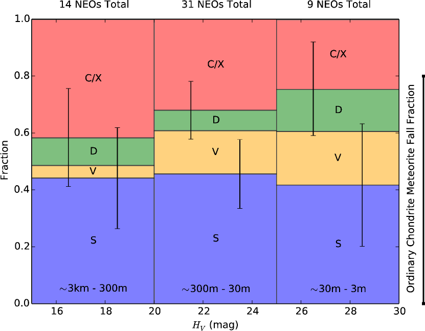
Figure 6: Compositional distribution of our target sample as a function of $H_{V}$, which serves as a proxy for target size (size scale assumes an average albedo of 0.15). With decreasing size, the fraction of C/X-type asteroids decreases, whereas the fraction of D-type and V-type asteroids seems to increase; based on Poisson statistics (error bars indicate 1$\sigma$ levels), both trends seem to be insignificant. The fraction of S-type asteroids is consistently lower than the expected ${\sim}80$% level derived from ordinary chondrite meteorite falls statistics (Harvey and Cassidy, 1989); S-type statistics agree with the 80% level at 2–3$\sigma$ for all size bins.

Based on our results in Table 2, we examine the compositional distribution of our sample as a function of absolute magnitude, which is used here as a proxy for the targets’ sizes. For this analysis, we only take into account sample targets with root-mean-square color uncertainties ${\leq}0.3$ that have not been marked in Table 2 for potential irregularities and cumulate the individual taxonomic classification probabilities. Taxonomic classification probabilities for targets with multiple observations have been averaged. We compare the fractions of individual taxonomic types in Figure 6 in three different $H_{V}$-ranges: $15<H_{V}\leq 20$ mag (14 objects), $20<H_{V}\leq 25$ mag (31 objects), and $25<H_{V}\leq 30$ (9 objects). With decreasing size (increasing $H_{V}$), we find a decreasing fraction of C/X-type NEOs and a relative increase in the fraction of D-type and V-type NEOs. Dealing with small sample sizes, we apply Poisson statistics to investigate the significance of these trends and for the sake of simplicity only consider the S and C/X complexes, which have the largest sample sizes. Figure 6 shows that the 1$\sigma$ uncertainties for S and C/X complex objects overlap in each size bin, which renders the decreasing trend of C/X complex objects with size insignificant. We also find the S-complex fraction to be independent of size at a level of 45%, which is in stark contrast to the finding that most meteorite falls are ordinary chondrites (${\sim}80$%, Harvey and Cassidy, 1989); ordinary chondrites are thought to originate from S-complex asteroids (Nakamura et al., 2011). Hinkle et al. (2014) independently find a similar discrepancy in MANOS data, suggesting a decreasing fraction of S-type asteroids with decreasing size. Taking the Poisson uncertainties into account, our S-complex fraction agrees at a 2–3$\sigma$ level with the fraction of ordinary chondrites for all size bins. Additional data will be necessary to improve statistics and investigate if this discrepancy is real. We note that our results do not account for bias inherent to our target sample. Being optically discovered, our sample targets are more likely to have medium to high surface albedos than low albedos, which favors S-complex over C/V-complex asteroids (e.g., Thomas et al., 2011). However, this effect would lead to an overestimation of the fraction of S-complex asteroids, suggesting that their real fraction is even lower. We postpone a detailed investigation of the compositional distribution of NEOs and a proper de-biasing of the distribution as a function of size to future work, which will be based on a larger sample.

We investigate the possibility that our rapid-response target selection introduces additional bias into our target sample, favoring specific taxonomic types. We test this hypothesis by comparing the distributions in semimajor axis, eccentricity, and inclination for our target sample and the sample of known NEOs (as reported by the Minor Planet Center as of 12 December 2015) using a two-sample Kolmogorov-Smirnov test. For each of the three parameters we find a $p$-value $>0.45$, indicating that we cannot reject the hypothesis that the distributions of the two samples are the same. Hence, our targets’ orbital parameter distribution does not significantly differ from the overall NEO distribution.

7 Conclusions and Future Outlook

Using rapid-response observations of NEOs in the near-infrared with UKIRT we are able to estimate taxonomic classifications for our sample targets in a simplified taxonomy scheme. Out of 110 observations of 104 different NEOs we derived reliable taxonomic classifications for 46 observations of 43 different NEOs; 18 observations had to be rejected because the target was too faint or the background too crowded, 25 more observations are subject to irregularities, 18 observations suffer from a low signal-to-noise ratio (color uncertainties ${>}0.3$ mag), and 7 observations lead to ambiguous taxonomic classifications (probabilities for all taxonomic classifications ${<}50$%). We expect a significantly higher efficiency in future observations after adjusting integration times. We find a good agreement between our taxonomic classifications and those derived from spectroscopic observations. We are able to reliably classify NEOs with $V\leq 21$ mag, which allows us to characterize asteroids down to a few meters in diameter, using our rapid-response approach. Our currently available data sample suggests that the fraction of S-complex asteroids in the NEO population is lower than the fraction of ordinary chondrites in meteorite fall statistics.

We will continue our observations with UKIRT and adapt our observing strategy based on the results of this work. In order to minimize the effect of galactic extinction on our $Z$ band calibration (see Section 2.2), we refrain from observing targets at galactic latitudes $|b|<15$°. Furthermore, we make $H$ band observations an integral part of our observations, as they provide additional information that improve the quality of our taxonomic classification, especially in cases in which a proper $Z$ band calibration is not possible from 2MASS data due to high levels of galactic extinction. We also adjust total integration times and filter sequences to provide the necessary photometric accuracy to minimize the classification uncertainties and improve the sensitivity of our survey.

References

- Bell et al. (2005) Bell, J. F., Owensby, P. D., Hawke, B. R. et al. 2005, NASA Planetary Data System, EAR-A-RDR-3-52COLOR-V2.1
- Bertin and Arnouts (1996) Bertin, E., Arnouts, S. 1996, A&AS, 117, 393
- Bertin et al. (2002) Bertin E., Mellier Y., Radovich M., Missonnier G., Didelon P., Morin B., 2002, ASP Conf. Series 281, 228
- Bertin (2006) Bertin E., 2006, in Astronomical Data Analysis Software and Systems XV, ASP Conf. Series 351, 112
- Bottke et al. (2002) Bottke, W. F., Morbidelli, A., Jedicke, R. et al., 2002, Icarus, 156, 399
- Brown et al. (2013) Brown, P. G., Assink, J. D., Astiz, L., Blaauw, R., Boslough, M. B. et al. 2013, Nature, 503, 238
- Casali et al. (2007) Casali, M., Adamson, A., Alves de Oliveira, C. et al. 2007, A&A, 467, 777
- DeMeo et al. (2009) DeMeo, F. E., Binzel, R. P., Slivan, S. M., Bus, S. M. 2009, Icarus, 202, 160
- Galache et al. (2015) Galache, J. L., Beeson, C. L., McLeod, K. K., Elvis, M. 2015, PaSS, 111, 155
- Gil-Hutton & Licandro (2010) Gil-Hutton, R., Licandro, J. 2010, Icarus, 206, 729
- Giorgini et al. (1996) Giorgini, J. D., Yeomans, D. K., Chamberlin, A. B. et al. 1996, Bulletin of the American Astronomical Society, 28, 1158
- Harvey and Cassidy (1989) Harvey, R. P., Cassidy, W. A. 1989, Meteoritics, 24, 9
- Hewett et al. (2006) Hewett, P. C., Warren, S. J., Legett, S. K. et al. 2006, MNRAS, 367, 454
- Hinkle et al. (2014) Hinkle, M. L., Moskovitz, N., Trilling, D. 2014, AAS, DPS meeting #46, #213.07
- Hinkle (2016) Hinkle, M. L. 2016, Master Thesis, Northern Arizona University
- Hodgkin et al. (2009) Hodgkin, S. T., Irwin, M. J., Hewett, P. C., Warren, S. J. 2009, MNRAS, 394, 675
- Howell (2006) Howell, S. B. 2006, Handbook of CCD astronomy, 2nd ed., Cambridge University Press, Cambridge, UK, ISBN 0521852153
- Irwin et al. (submitted) Irwin, M., Lewis, J., Riello, M. et al. 2006, submitted to MNRAS
- Lawrence et al. (2007) Lawrence, A., Warren, S. J., Almaini, O.] et al. 2007, MNRAS, 379, 1599
- Leggett et al. (2006) Leggett, S. K., Currie, M. J., Varricatt, W. P., Hawarden, T. G., Adamson, A. J. et al. 2006, MNRAS, 373, 781
- Moskovitz et al. (2015) Moskovitz, N. A., Burt, B., Binzel, R. P., Christensen, E., DeMeo, F. et al. 2015, LPI Contribution No. 1829, 6038
- Nakamura et al. (2011) Nakamura, T., Noguchi, T., Tanaka, M., Zolensky, M. E., Kimura, M. et al. 2011, Science, 333, 1113
- Pedregosa et al. (2011) Pedregosa, F., Varoquaux, G., Gramfort, A. et al. 2011, Journal of Machine Learning Research, 12, 2825
- Popova et al. (2013) Popova, O. P., Jenniskens, P., Emel’yanenko, V., Kartashova, A., Biryukov, E. et al. 2013, Science, 342, 1069
- Rayner et al. (2003) Rayner, J. T., Toomey, D. W., Onaka, P. M. et al. 2003, PASP, 115, 362
- Skrutksie et al. (2006) Skrutskie, M. F., Cutri, R. M., Stiening, R., Weinberg, M. D., Schneider, S. et al. 2006, AJ, 131, 1163
- Sykes et al. (2000) Sykes, M. V., Cutri, R. M., Fowler, J. W. et al. 2000, Icarus, 146, 161
- Thomas et al. (2011) Thomas, C. A., Trilling, D. E., Emery, J. P., Mueller, M., Hora, J. L. et al. 2011, AJ, 142, 85
- Warner (2015a) Warner, B. D. 2015,Minor Planet Bul. 42, 41
- Warner (2015b) Warner, B. D. 2015, Minor Planet Bul. 42, 115
- Zellner et al. (1985) Zellner, B., Tholen, D. J., Tedesco, E. F. 1985, Icarus, 61, 355