Fundamental frequencies and resonances from eccentric and precessing binary black hole inspirals

Abstract

Binary black holes which are both eccentric and undergo precession remain unexplored in numerical simulations. We present simulations of such systems which cover about 50 orbits at comparatively high mass ratios 5 and 7. The configurations correspond to the generic motion of a nonspinning body in a Kerr spacetime, and are chosen to study the transition from finite mass-ratio inspirals to point particle motion in Kerr. We develop techniques to extract analogs of the three fundamental frequencies of Kerr geodesics, compare our frequencies to those of Kerr, and show that the differences are consistent with self-force corrections entering at first order in mass ratio. This analysis also locates orbital resonances where the ratios of our frequencies take rational values. At the considered mass ratios, the binaries pass through resonances in one to two resonant cycles, and we find no discernible effects on the orbital evolution. We also compute the decay of eccentricity during the inspiral and find good agreement with the leading order post-Newtonian prediction.

1 Introduction

The recent landmark detections of gravitational waves by the Advanced LIGO interferometers gave definitive proof that binary black hole (BBH) systems exist and merge in nature [1, 2, 3]. Detection and characterization of the resulting signals relies on knowledge of the expected gravitational waveforms for tasks as varied as detection, parameter estimation, and tests of general relativity [4]. The use of theoretical waveforms enhances gravitational wave (GW) astronomy’s scientific potential where waveform models are available, as demonstrated by the GW detections and analyses in Advanced LIGO’s first observing run [5]. Conversely, the absence of accurate and reliable waveform models may limit detection sensitivity, and hinders source parameter estimation and tests of gravitational theories.

Due to both physical motivations and computational complexity, waveform modeling for BBH systems has focused on quasi-circular binaries. Orbital eccentricity is damped away quickly during a GW-driven inspiral of two compact objects [6] because GW emission peaks at periastron. Thus “field binaries” formed from the respective collapse of both partners in a high-mass stellar binary are expected to be almost exactly circular by the time they enter the sensitive band of ground-based GW detectors. Quasi-circularity removes the two degrees of freedom related to orbital eccentricity, and thus reduces the dimensionality of the BBH parameter space that needs to be modelled. Mature waveform models exist for quasi-circular, aligned-spin BBH systems [7, 8], while models of quasi-circular BBH systems with generic spin (i.e. precessing binaries) are maturing quickly (e.g. [9, 10, 11]). These waveform models are based on direct numerical solutions of Einstein’s equations (e.g. [12]) that provide the gravitational waveforms for the late inspiral and merger of the two black holes; such numerical simulations, too, are most mature for quasi-circular systems (e.g. [13, 14, 15, 16, 17, 18]).

In contrast, very few numerical simulations have been performed for eccentric BBH systems [19, 20, 21, 22, 23, 24], and a systematic numerical exploration of the eccentric parameter space has not even started. Complete inspiral-merger-ringdown waveform models for eccentric BBH systems are also in a nascent state, with current models [25] neither reaching the accuracy of quasi-circular models, nor accounting for black hole spins (not even aligned-spin).

Several astrophysical scenarios have been explored in recent years which can lead to nonzero eccentricity late in the inspiral: Within dense stellar environments such as globular clusters (GCs) and galactic cores, binaries can form dynamically (e.g. [26, 27, 28, 29]), and there can be significant residual eccentricity from direct dynamical capture [30, 31, 32, 33]. The scattering of single stars off binaries [34] can also lead to high eccentricities, although these events are likely rare [35]. Even more promisingly, eccentricity can be generated by the Kozai-Lidov mechanism [36, 37, 38, 39, 40, 41, 42] in three body systems with moderate separations [43, 44, 45, 46, 47]. Such triples can occur in GCs [48, 35] or galactic nuclei [43], and may provide a source for eccentric compact binaries in advanced detectors [49, 50, 35] (in particular reference [35] estimates $e>0.1$ should occur at rate of about 0.2 yr^-1, but see also [51]).

Ultimately gravitational wave observations will be the primary tool to measure eccentricity of compact object inspirals and to constrain the rate of eccentric compact mergers. Unfortunately, the present detection template bank used by LIGO is entirely circular [5, 52], hindering detection of systems with in-band eccentricities above about $e\sim 0.1$ [53, 54, 25]. Due to this same absence of eccentric waveform models, parameter estimation must likewise assume quasi-circularity.

Looking ahead, the “extreme mass-ratio inspirals” (EMRIs) visible to space-based detectors such as LISA [55, 56] may be detected at quite large eccentricities (e.g. [57]). While eccentric waveforms are being developed [25, 58], further numerical and analytical modeling of eccentric systems are required to constrain eccentricity and prepare for future ground- and space-based detections of eccentric systems.

Eccentric systems also yield additional insight into strong-field dynamics, especially at high mass ratios [59, 60, 61]. While circular orbits must remain outside the innermost stable circular orbit (ISCO) until the final plunge, eccentric orbits can reach as deep as the innermost bound orbit, thus probing stronger gravitational fields [62]. Furthermore, binaries which are both eccentric and precessing open up the possibility of qualitatively new phenomena when orbits pass through resonances and radiation reaction effects accumulate secularly [63, 64].

This paper presents a survey of 12 numerical simulations over a range of initial eccentricities as high as $e=0.2$, mass ratios $q=5$ and $7$, and initial inclinations between the spin and the orbital plane between $0^{\circ}$ and $80^{\circ}$, performed with the Spectral Einstein Code (SpEC) [65]. We focus on higher mass ratios in order to make contact with the extreme mass ratio limit, where the BBHs can be modelled to leading order by bounded motion of a test particle in a Kerr spacetime. Beyond the test particle limit, the motion is corrected by higher order, self-force (SF) effects due to the spacetime perturbations sourced by the particle [66]. In this case the ratio of the particle mass $\mu$ to that of the Kerr black hole $M_{\rm Kerr}$ serves as a small expansion parameter. While SF results for Kerr are still in development [67, 68, 69, 70], mounting evidence suggests that SF results may be extended much closer to the nearly equal mass cases than expected [71, 72, 73], which is the regime appropriate for our our high (but not extreme) mass ratio binaries. Meanwhile, the lowest order approximation to the SF-expansion, namely the test particle limit, incorporates the effects of strongly curved spacetime, highly relativistic motion, and is fully understood. At the same time, post-Newtonian approximations have difficulty describing higher mass ratio binaries, where the constituents remain at close separations for many orbits. In addition, higher mass ratio binaries can potentially remain at orbital resonances for multiple cycles of the resonance, and our simulations allow for the first investigation of the role of passage through resonances in BBHs.

In order to compare to the test particle limit and investigate these SF corrections, our primary interest is the computation of the characteristic frequencies in the azimuthal ($\Omega^{\phi}$), radial ($\Omega^{r}$), and polar ($\Omega^{\theta}$) directions. Except very close to ISCO these frequencies furnish a one-to-one map with (self-force corrected) Kerr geodesics [74] and thus provide a natural point of comparison with the latter. In the Kerr spacetime the effect of timelike coordinate transformations that do not involve time-dependent rotations is to multiply all of the frequencies by the same factor [75]. Thus their ratios $K^{ab}\equiv\Omega^{a}/\Omega^{b}$ are insensitive to such transformations. In the particular case of nearly circular orbits, the periastron precession rate of BBHs simulations as encoded in $K^{r\phi}$ was investigated [71, 73], showing that analytic approximations provide highly accurate descriptions of the simulations. Additionally, the precession rates $K^{ab}$ are of interest because the points in the orbit when these frequency ratios are rational are precisely the moments of orbital resonance. Their extraction can be used to characterize and explore such resonances in our simulations.

Extracting the characteristic frequencies accurately from an eccentric, precessing numerical relativity simulation turns out to be challenging due to both strong dissipation as well as modulations arising from interactions of radial and polar motion. Fourier-based methods of frequency extraction require several orbits to achieve percent level accuracy, resulting in unacceptable dissipative contamination. We therefore rely upon time-domain methods based on intervals between successive periastron passages, which achieve better accuracy with only a single orbit.

This paper is structured as follows. In section 2 we introduce the basic context of our analysis by discussing generic test orbits in the Kerr spacetime. In section 3 we review the simulations we have performed in detail and describe the association we make between simulation trajectories and Kerr geodesics. In section 4 we detail our frequency extraction methodology and its results for our equatorial runs. Section 5 provides the same analysis for the inclined runs, and showcases our ability to detect resonances in these simulations. We discuss our results and future directions in section 6.

2 Motion in Kerr spacetimes

We interpret our high mass ratio, eccentric, and precessing simulations in terms of motion in the Kerr spacetime. From the perspective of dynamical systems, bound test orbits in Kerr form an integrable Hamiltonian system. Such systems admit action-angle coordinates, in which the generalized momenta are the conserved actions $J^{a}$. The conjugate positions are circulating angles which evolve at fixed frequencies. The motion of the particle is multiperiodic, and can be expanded in a Fourier series in the frequencies. In Hamiltonian perturbation theory the action-action angle formalism elucidates the perturbed motion, the loss of integrability, and the onset of chaos [76].

For Kerr geodesics, the transformation to action-angle variables was first discussed by Schmidt [75]. The resulting $J^{a}$ are geometric invariants, and the associated proper time frequencies describe the motion in a coordinate-independent manner. The frequencies measured by alternative observers are related to the proper time frequencies through multiplication by a Lorentz-like factor. In particular, distant inertial observers measure frequencies $\Omega^{a}$.

Self-force corrections to geodesic motion decompose usefully into conservative corrections to the orbital dynamics and dissipative effects which drive inspiral [77]. The small size of the dissipation means that this system is amenable to evolution using a two-timescale approach [78, 79]. We work in the paradigm where (accounting for the slow dissipation) the fundamental frequencies are perturbed by the conservative SF effects. This perturbed Hamiltonian perspective on the SF problem has been used to compute invariant quantities in Kerr spacetimes [80]. Our goal in sections 4 and 5 is to extract the fundamental frequencies from our simulations, which have physical meaning in terms of precession rates of the binary as viewed by distant, inertial observers. The differences between these frequencies and those of Kerr can be viewed as (possibly high-order) self-force corrections; thus our work may be useful for comparison with future self-force results.

2.1 Geodesic orbits in Kerr

A test particle on a bound orbit in the Kerr spacetime has four conserved quantities: the specific energy $\mathcal{E}$, the specific angular momentum along the symmetry axis $\mathcal{L}_{z}$, the specific Carter constant $\mathcal{Q}$, and the Hamiltonian constraint $\mathcal{H}=(1/2)g^{\mu\nu}p_{\mu}p_{\nu}=-\mu^{2}/2$, where $\mu$ denotes the mass of the test particle. It is convenient to use Boyer-Lindquist coordinates $x^{\mu}=(t,r,\theta,\phi)$ (see A) and to define the Carter-Mino time $\lambda$ through [82, 77]

$$\frac{d\tau}{d\lambda}=\rho^{2}\,,\qquad\rho^{2}=r^{2}+a^{2}\cos^{2}\theta\,,$$ (1)

where $\tau$ is the proper time of the trajectory. Parameterized by $\lambda$ rather than $\tau$, the equations for the radial and polar motions of the particle separate,

$$\left(\frac{dr}{d\lambda}\right)^{2}=R(r)\,,\qquad\left(\frac{d\theta}{d\lambda}\right)^{2}=\Theta(\theta)\,,$$ (2)

where the potentials $R$ and $\Theta$ are given in (28) and (29). This results in independent cyclic motions in the $r$ and $\theta$ directions.

Unfortunately, the equations of motion for $t(\lambda)$ and $\phi(\lambda)$ depend on both the radial and polar motions,

$$\frac{dt}{d\lambda} = T_{r}(r)+T_{\theta}(\theta)+a\mathcal{L}_{z}\,,$$ (3)

$$\frac{d\phi}{d\lambda} = \Phi_{r}(r)+\Phi_{\theta}(\theta)-a\mathcal{E}\,,$$ (4)

with the potentials on the right hand side given by (30) and (31). This means that $r(t)$, $\theta(t)$, and $\phi(t)$ are multiperiodic, complicating the extraction of the fundamental frequencies of motion. For geodesics, this problem can be solved by moving to action-angle coordinates [75].

When studying bound orbits it is useful to introduce a Keplerian parametrization of the orbit, which represents the radial motion as a precessing eccentric orbit. The radius evolves as

$$r=\frac{pM}{1+e\cos\chi^{r}}\,,$$ (5)

where $p$ and $e$ respectively denote the semilatus rectum and eccentricity of the orbit. The phase $\chi^{r}(\lambda)$ represents the position of the particle along the precessing ellipse. The particle oscillates between the periastron $r_{p}=p/(1+e)$ and apastron $r_{a}=p/(1-e)$. Similarly, one can express the polar motion as an oscillation between symmetric turning points above and below the equatorial plane, by writing [83, 84]

$$\cos\theta\equiv\cos\theta_{\rm min}\cos\chi^{\theta}\,,$$ (6)

where $\theta_{\rm min}$ is the smallest polar angle the particle reaches at the height of its vertical motion. We define the inclination of the orbit by $i=\pi/2-\theta_{\rm min}$ as the inclination angle of the orbit above the equatorial plane. Note that our use of $i$ to define the inclination angle of our orbit differs from the commonly used (e.g. [85]) inclination angle $\iota$ defined through the constants of motion by $\cos\iota=\mathcal{L}_{z}/(\mathcal{Q}+\mathcal{L}_{z}^{2})^{1/2}.$

Together, $(p,e,i)$ characterize bound orbits. Given these orbital parameters, we can compute the corresponding constants of motion $(\mathcal{E},\mathcal{L}_{z},\mathcal{Q})$ [75] and solve the equations of motion, see e.g. [84].

2.2 Fundamental frequencies of Kerr

In the case of equatorial, eccentric orbits, the fundamental frequencies are straightforward to define. The particle oscillates between periastron and apastron, while advancing in the azimuthal angle $\phi$. The two relevant frequencies are the frequency between successive radial passages, $\Omega^{r}$, and the azimuthal frequency averaged over successive passages, $\Omega^{\phi}$.

The frequency ratio $K^{r\phi}=\Omega^{r}/\Omega^{\phi}$ measures the periastron precession rate. It is a well-defined observable that can be measured by distant inertial observers, for whom the particular coordinate time that the frequencies reference (whether it be $t$, $\tau$, or $\lambda$) divides out.

For generic, non-equatorial orbits the situation is more complicated. In terms of $\lambda$ the radial and polar motions decouple. However, azimuthal motion is modulated by both the radial and polar motions. Similarly, the Boyer-Lindquist time $t(\lambda)$ along the world line is modulated by the radial and polar motions. This results in multiperiodic behaviour in the coordinate graphs: the time between successive coordinate extrema is variable, and only the long-term average time between extrema approaches the fundamental periods $T^{a}=2\pi/\Omega^{a}$.

Thus the fundamental frequencies $\Omega^{r}$, $\Omega^{\theta}$, $\Omega^{\phi}$ are infinite time averages. Once again, the ratios of frequencies $K^{r\phi}$, $K^{r\theta}=\Omega^{r}/\Omega^{\theta}$, and $K^{\theta\phi}=\Omega^{\theta}/\Omega^{\phi}$ eliminate the dependence on the particular choice of time coordinate, and are related to the precession rates of the periastron and of the instantaneous orbital plane.

We use the method of Schmidt [75] to compute the fundamental frequencies in terms of our chosen time parameter. Fujita and Hikida [84] provide analytic solutions for the bound orbits and their fundamental frequencies in terms of elliptic integrals. We do not exploit these, instead numerically integrating the geodesic equations to validate our frequency extraction methods discussed in section 3. We choose to use frequencies $\Omega^{a}$ in terms of Boyer-Lindquist time $t$. The precise choice of time-coordinate will cancel in the frequency ratios, so long as the coordinates under study do not differ by time-dependent rotations.

2.3 Orbital resonances

Unlike the familiar quasi-circular inspirals, eccentric and especially eccentric, precessing systems can access the qualitatively new dynamical effect of orbital resonances. These occur when the fundamental frequencies $\Omega^{a}$ are in (or near) rational ratio. In that case the trajectory is exactly (or approximately) closed in phase space and perturbations can accumulate secularly. During resonance the perturbed system’s evolution can deviate dramatically from its unperturbed counterpart. In the generic case of a Hamiltonian system this leads to “islands” of chaotic motion in the phase space. When dissipation is included perturbed systems pass through resonances. This may lead to distinct changes in the evolution of the frequency ratios (see, e.g. [86]), the resonant “kicks” discussed below, or even capture into the resonance [87, 88]. If the passage is fast enough, however, the system may not display chaotic behaviour or other signatures of resonant passage. For late-inspiral BBH systems no evidence for such chaotic motion has been observed, presumably since the dissipative timescales are too short for any significantly ergodic motion to manifest.

Resonances can nevertheless have an important effect on the motion of high mass-ratio systems, due to concordant asymmetries in the gravitational radiation reaction. The emission of energy, momentum, and angular momentum to infinity is controlled by the Weyl scalar $\Psi_{4}$, which when sourced by bound orbits in Kerr can be Fourier expanded as [83]

$$\Psi_{4}=\frac{1}{(r-ia\cos\theta)^{-4}}\sum_{lmkn}R_{lmkn}(r)S_{lmkn}(\theta)e^{im\phi-\Omega_{mkn}t}\,,$$ (7)

where $R_{lmkn}(r)$ is the radial wave function which solves the sourced radial Teukolsky equation [89], $S_{lmkn}(\theta)$ are the spin-weight $s=-2$ spheroidal harmonics, and

$$\Omega_{mkn}=m\Omega^{\phi}+n\Omega^{\theta}+k\Omega^{r}\,.$$ (8)

Fluxes to infinity are built from the time integrals of $|\Psi_{4}|^{2}$, followed by angular integrals over the sphere at infinity, possibly weighted by additional angular terms. The result is interference between harmonics $(m,n,k)$ and $(m^{\prime},n^{\prime},k^{\prime})$. Typically the interference oscillates rapidly and does not contribute to the time integral. For example, for the flux of energy only terms where $(m,n,k)=(m^{\prime},n^{\prime},k^{\prime})$ contribute.

At resonances, however, the generically-unimportant terms accumulate, leading to resonantly enhanced or diminished fluxes [64]. Resonances can also lead to gravitational wave beaming: during resonance the BBH trajectory (or its projection into the $r$-$\theta$ plane) closes on itself, taking the form of a Lissajous figure. That figure need not be symmetric in space, and gravitational wave emission need not be symmetric either. These resonant kicks have been studied for circular, precessing orbits at $\theta$-$\phi$ resonances [90], and for equatorial, eccentric orbits at $r$-$\phi$ resonances [91]. In these studies, the resonances required for symmetry breaking of the orbit are high order and occur only for very close orbits. For example, the $r$-$\phi$ kicks require $K^{r\phi}=1/p$ with $p$ an integer and $p\geq 2$; such orbits are zoom-whirl orbits. Initial investigation in [91] indicated that $r$-$\phi$ kicks are relatively strong and may be effective for inspirals with mass ratios $q=m_{1}/m_{2}\gtrsim 5$. However, these kicks require that a finite mass ratio inspiral achieve these extreme orbits before plunge and merger.

Resonant kicks do not lead to chaotic motion since their influence is self-limiting: the dissipation will inevitably push the inspiral off the resonant trajectory. At this point the system will resume its approximately adiabatic motion. Nevertheless the precise kick dynamics depend sensitively on the orbital phase at which the binary enters resonance. This would challenge a description of systems undergoing resonant kicks using e.g. a template bank of gravitational waveforms.

Of particular interest are the resonances between radial and polar motion described in [64, 92]. These resonances cause secular accumulation in SF effects and drive a rapid change in the conserved quantities, especially the Carter constant $\mathcal{Q}$. In the extreme mass-ratio limit $\mu/M\to 0$ an $O(1)$ change to the phase prior to resonance leads to an $O(\sqrt{M/\mu})$ correction to the phase post-resonance. Importantly, these resonances are effective at many more resonant frequencies than the kicks. Any rational ratio for $\Omega^{r}$ and $\Omega^{\theta}$ will do, although lower order resonances like $2$:$3$ or $3$:$4$ are expected to have a larger effect than higher orders. Systems passing through successive $r$-$\theta$ resonances could accumulate a sensitive dependence on initial conditions.

While resonances are a high mass-ratio effect, the precise value of $q$ at which they may become important is as yet unknown, partly due to the current absence of any systematic numerical studies of eccentric inclined black hole binaries. It is indeed possible that resonances may become relevant at the mass ratios accessible, or nearly accessible, to numerical relativity. This would potentially seriously frustrate attempts by LIGO to measure moderate mass-ratio eccentric inspirals using matched filtering. In sections 4 and 5 we test to see whether the high mass ratio, eccentric and generic inspirals we discuss in section 3 display interesting resonant behaviour.

3 Numerical relativity simulations

3.1 Simulations of eccentric, precessing black hole binaries

We perform simulations with the Spectral Einstein Code [93], which uses a generalized harmonic formulation [94, 95, 96, 97] to integrate the Einstein equations in damped harmonic gauge [98, 99, 100]. The code uses an adaptively refined grid [101] between two sets of boundaries. Lying within the holes, the “excision boundaries” are chosen to conform to the shapes of the apparent horizons [100, 102, 103, 104]. After merger there is only one excision boundary [102, 103]. Being inside the holes, the excision boundaries are pure-outflow and no boundary conditions are required. The grid extends from the excision boundaries to an artificial outer boundary endowed with constraint-preserving boundary conditions [97, 105, 106]. The evolution proceeds from the construction [107] of quasi-equilibrium [108, 109] initial conditions satisfying the Einstein constraint equations [110].

We run each of our simulations at three resolutions, which we label L1 (lowest resolution), L2, and L3 (highest resolution). Each choice of resolution provides different tolerances on the adaptive mesh refinement. Each resolution thus has a different refinement history. While this prevents us from showing strict convergence of quantities extracted from the simulations, the range quantities take over the three resolutions is a measure of our numerical error. When it is practical we plot all three resolutions, and when we report a single result from a given simulation it is from the highest resolution, L3. All of our results are consistent across resolutions.

We label the masses of our black holes $m_{1}$ and $m_{2}$, using the convention that $m_{1}>m_{2}$. The total mass of the black holes $M=m_{1}+m_{2}$ sets all scales in our simulations. Our black holes have angular momenta ${\bm{S}}_{1}$ and ${\bm{S}}_{2}$, computed using quasi-local angular momentum diagnostics [109, 111], and we define dimensionless spin vectors through ${\bm{\chi}}_{i}={\bm{S}}_{i}/m_{i}^{2}$, where here $i=1,2$ labels the black holes. We focus on two sequences of simulations. One sequence has mass ratio $q=m_{1}/m_{2}=5$ and $\chi_{1}=|{\bm{\chi}}_{1}|=0.6$, and the other sequence has $q=7$ with $\chi_{1}=0.8$. In both cases, we set ${\bm{\chi}}_{2}=0$. These parameters were chosen so that the binary orbits might be modelled by motion in Kerr spacetime with mass $m_{1}$ and spin parameter $\chi_{1}$, together with radiation reaction effects and finite mass ratio corrections to the motion. By selecting two choices of BH parameters we have some freedom to investigate the effect of varying those parameters while keeping computational expense manageable.

For our two choices of $(q,\chi_{1})$ we ran two sets of simulations, using “low” and “high” initial eccentricities. We targeted the initial eccentricities by using simple Keplerian relations between the initial orbital separation and angular velocity of the binary at the moment of apastron passage, where we began our simulations. Specifically, the initial data solver takes as input an initial expansion factor $\dot{a}_{0}$, an initial orbital frequency $\Omega_{0}$, and an initial coordinate separation distance $D_{0}$. We set $\dot{a}_{0}$ to zero in all cases, to fix the orbit at apastron. For a given initial distance $D_{0}$, we target a Newtonian eccentricity $e_{N}$, using the so-called “vis-viva” equation (which expresses energy conservation for the orbit) at apastron,

$$\Omega_{0}^{2}=(m_{1}+m_{2})\left(\frac{1-e_{N}}{D_{0}^{3}}\right)\,,$$ (9)

to solve for the appropriate $\Omega_{0}$. We chose $e_{N}=0.2$ for our “low eccentricity” and $e_{N}=0.3$ for our “high” eccentricity runs.

The initial separation $D_{0}$, together with the achieved eccentricity $e$ and the mass ratio $q$, controls the length of the inspiral. In order to facilitate accurate frequency extraction we set the simulations to be quite long, using initial distances $D_{0}$ of $19.5M$ and $21.125M$. This gave the same initial Newtonian semi-major axis of $D_{0}/(1+e_{N})=16.25M$ for all of our simulations, and they proceeded through $\approx 30-60$ radial oscillations before merger.

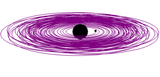
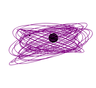
Figure 1: Coordinate trajectories for two $q=7$, $\chi_{1}=0.8$, high eccentricity simulations. Left: An equatorial inspiral, depicted up to the final orbit before merger. Right: About $28$ periastron passages from the middle of an inspiral with a $40^{\circ}$ inclination. Both panels show a 3-dimensional perspective view.

To investigate the effects of precession we ran each simulations for each of the above choices of $(q,\chi_{1})$ and $e_{N}$ three times, initializing the spin vector ${\bm{\chi}}_{1}$ to form angles of $0^{\circ}$, $10^{\circ}$, and $20^{\circ}$ with the computational $z$-axis in the $q=5,\chi_{1}=0.6$ cases and $0^{\circ}$, $40^{\circ}$, and $80^{\circ}$ in the $q=7$, $\chi_{1}=0.8$ cases. The $z$-axis is normal to the initial orbital plane. These choices of initial inclinations of the orbital plane to the spin of the more massive hole spans the full range of orbits from the perspective of motion in Kerr, from equatorial to near-equatorial to nearly polar orbits. Figure 1 plots the trajectories for portions of two of our $q=7$, high eccentricity orbits.

In table 1 we present the full range of simulation parameters. The number of radial oscillations before merger $\mathcal{N}_{r}$ is estimated by counting the number of maxima in the coordinate separation $r$ of the centers of the black holes, following the initial junk phase. The number of orbits $\mathcal{N}_{\phi}$ is estimated by integrating the orbital frequency $\Omega(t)$ defined in (10) below over the entire inspiral. For our precessing runs, this $\mathcal{N}_{\phi}$ does not correspond to the number of azimuthal cycles in the fixed simulation coordinates, since $\Omega(t)$ is the angular velocity in the instantaneous, precessing orbital plane. Computation of the simulation eccentricity $e$ [and thus its initial eccentricity $e_{0}=e(t=0)$] is described below in section 3.2; the expression for $e(t)$ is given by (14). The target eccentricity $e_{N}$ turns out to produce an overestimate of the initial eccentricity $e_{0}$, but one which is stable across our simulations.

Table 1: Simulations used in this study. Tabulated here are mass-ratio $q$, dimensionless spin ${\bm{\chi}}_{1}$ of the larger black hole, initial separation $D_{0}$, initial orbital frequency $\Omega_{0}$, the Newtonian eccentricity $e_{\rm N}$ used to choose $\Omega_{0}$, the actual eccentricity of the simulation at its start $e_{0}$, and the initial inclination $i$. The last two columns report the number of azimuthal and radial cycles during the inspiral.

Run	$q$	${\bm{\chi}}_{1}$	$D_{0}$	$\Omega_{0}\times 10^{2}$	$e_{\rm N}$	$e_{0}$	$i$	$\mathcal{N}_{\phi}$	$\mathcal{N}_{r}$
q5_i00_low-e	5	$(0,0,0.6)$	19.5	1.0387	0.2	0.07689	$0^{\circ}$	55	41
q5_i10_low-e	5	$(-0.10419,0,0.59089)$	19.5	1.0387	0.2	0.07700	$10^{\circ}$	55	42
q5_i20_low-e	5	$(-0.20521,0,0.56382)$	19.5	1.0387	0.2	0.07749	$20^{\circ}$	54	41
q5_i00_high-e	5	$(0,0,0.6)$	21.125	0.8617	0.3	0.2126	$0^{\circ}$	42	31
q5_i10_high-e	5	$(-0.10419,0,0.59089)$	21.125	0.8617	0.3	0.2128	$10^{\circ}$	42	31
q5_i20_high-e	5	$(-0.20521,0,0.56382)$	21.125	0.8617	0.3	0.2134	$20^{\circ}$	41	31
q7_i00_low-e	7	$(0,0,0.8)$	19.5	1.0387	0.2	0.06657	$0^{\circ}$	74	59
q7_i40_low-e	7	$(-0.51423,0,0.612836)$	19.5	1.0387	0.2	0.06942	$40^{\circ}$	72	58
q7_i80_low-e	7	$(-0.787846,0,0.138919)$	19.5	1.0387	0.2	0.07954	$80^{\circ}$	60	46
q7_i00_high-e	7	$(0,0,0.8)$	21.125	0.8617	0.3	0.2032	$0^{\circ}$	60	45
q7_i40_high-e	7	$(-0.51423,0,0.612836)$	21.125	0.8617	0.3	0.2069	$40^{\circ}$	55	42
q7_i80_high-e	7	$(-0.787846,0,0.138919)$	21.125	0.8617	0.3	0.2195	$80^{\circ}$	44	32

3.2 Dynamics of simulated binaries

In order to connect our simulations with analytic theory we need to first construct quantities that can be used to extract fundamental frequencies. Numerical simulations yield the position vectors ${\bm{x}}_{1}(t)$ and ${\bm{x}}_{2}(t)$ of the Cartesian coordinate-centres of the holes, and a spin-vector ${\bm{\chi}}_{1}(t)$ describing the spin angular momentum of the more massive hole.

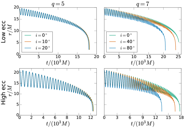
Figure 2: Coordinate separations of our BBH simulations as a function of simulation time. The simulations are grouped into four panels according to mass-ratio (left, $q=5$; right, $q=7$) and eccentricity (top, low eccentricity; bottom, high eccentricity). Each panel shows runs at the three different inclinations $i$.

From the position vectors we compute a radial separation vector ${\bm{r}}(t)\equiv{\bm{x}}_{1}(t)-{\bm{x}}_{2}(t)$ along with its magnitude $r\equiv|{\bm{r}}|$. The separation $r$ has no invariant meaning, but it illustrates the dynamics of the inspiral; we thus plot it in figure 2. The number of extrema of $r$ indicate the number of apastron and periastron passages, and the decline in eccentricity during the inspiral is evident in the decreasing amplitude of the oscillations of $r$.

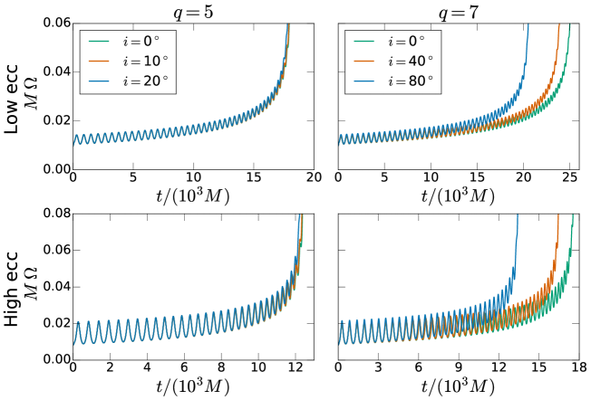
Figure 3: Orbital frequency $\Omega$ from (10) as a function of simulation time, organized in the same way as in figure 2.

For the equatorial runs we do not work with ${\bm{r}}$ directly. Instead we compute from it an orbital frequency [112]

$$\Omega(t)\equiv\frac{|{\bm{r}}\times\dot{\bm{r}}|}{r^{2}}\,,$$ (10)

from which we are able to extract the fundamental frequencies $\Omega^{\phi}(t)$ and $\Omega^{r}(t)$. In practice, we compute $\dot{\bm{r}}=d{\bm{r}}/dt$ with a 3rd order Savitzky-Golay filter windowed over groups of seven points [113]. Our time coordinate is asymptotically inertial [114], justifying our identification of simulation coordinate frequencies with those measured by asymptotic, inertial observers.

In figure 3 we plot $\Omega(t)$ for our simulations, which clearly shows modulations due to the eccentricity. The modulation amplitude decreases throughout the inspiral as eccentricity is radiated away. The modulations are not simple sinusoidal oscillations about a chirping mean, but instead exhibit sharper peaks at periastron, an effect more pronounced at higher eccentricities.

Our analysis of eccentric motion is based on the oscillatory features of $\Omega(t)$. For non-dissipative orbits, one would simply utilize the extrema of $\Omega(t)$. However, as shown in figure 3, GW-driven inspiral adds an overall monotonic trend to the radial motion of the binary, so that extrema of $\Omega(t)$ do not correspond precisely to the reversals of the underlying oscillatory behavior. Should the growth rate of the monotonic trend ever exceed the range of the growth rate of the oscillatory one, as can easily happen at late inspiral, or even early inspiral when eccentricity is low, $\Omega(t)$ will no longer display extrema at all.

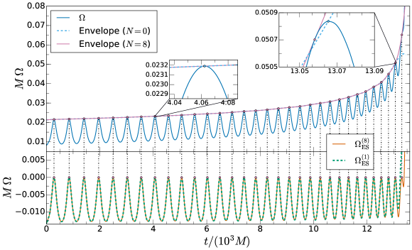
Figure 4: Illustration of refinement procedure applied to $\Omega$ from (10) computed from our q7_i80_high-e run. The top panel shows $\Omega$ itself, while the bottom shows the same after $N=1$ and $N=8$ iterations of envelope subtraction, when the location of the maxima are stable up to machine precision. The refined curve is computed by subtracting a 4th order spline interpolation of the maxima (the “envelope”) from the original curve; each iteration denotes a subsequent envelope subtraction from the result of this procedure. This results in an envelope which, rather than passing through the maxima of the original curve, lies tangent to it, as seen in the inserts. The difference between the maxima of each iteration is due to dissipation and thus becomes more pronounced further into the inspiral. The refinement procedure also sometimes finds additional peaks which were saddle points in the original curve (note the differences between the envelopes as well as the $\Omega_{\rm ES}^{(N)}$ curves close to the end of the inspiral).

We begin by computing the maxima and minima of $\Omega(t)$. We denote the times where $\Omega(t)$ takes its maximum and minimum values as $t_{i}^{+}$ and $t_{i}^{-}$, respectively, where $i$ labels successive maxima/minima. For a conservative orbit these extrema are precisely the points of physical interest and the procedure is complete.

For inspiraling orbits, we apply a refinement procedure based on the subtraction of the envelope of the upper extrema. This procedure is motivated by analyzing a simple model in B and is illustrated in figure 4. We compute a spline-fit to the extrema $\{(t_{i}^{+},\Omega(t_{i}^{+}))\}$, and subtract this fit from $\Omega(t)$. This results in the first-stage ($N\!=\!1$) “envelope subtracted” frequency $\Omega_{\rm ES}^{(1)}(t)$, cf. the lower panel of figure 4. We now iterate this procedure: Find the abscissas of the maxima of $\Omega_{\rm ES}^{(1)}(t)$; compute a spline-fit to the respective points in $\Omega(t)$; subtract to generate the $N\!=\!2$ envelope subtraction, $\Omega_{\rm ES}^{(2)}(t)$. We iterate the procedure $N_{f}$-times until no more change occurs to within machine precision (typically $N_{f}\!=\!8$). We redefine the extremal times $t^{+}_{i}$, $t^{-}_{i}$ as the maxima/minima of $\Omega_{\rm ES}^{(N_{f})}(t)$. We finally define $\Omega^{\pm}(t)$ as the spline-interpolant to $\{(t_{i}^{\pm},\Omega(t_{i}^{\pm}))\}$. (In practice, we are most interested in $\Omega^{+}$ when computing radial frequencies, since the sharper peaking of $\Omega(t)$ at periastron allows the former to be located more accurately.) Envelope-subtraction generates a spline-interpolant $\Omega^{+}(t)$ which appears tangent to the original $\Omega(t)$, whereas the original envelope passing through the bare peaks would cross it (cf. the upper right inset of figure 4). During our analysis of inclined runs in section 5 we use an envelope-subtracted separation

$$r_{\rm ES}(t)\equiv r(t)-r^{+}(t),$$ (11)

which is generated with the identical procedure, substituting $r(t)$ for $\Omega(t)$ above.

Figure 5: Eccentricity vs. orbital frequency for our numerical simulations (solid lines). The simulations are grouped into four panels according to mass-ratio (left, $q=5$; right, $q=7$) and initial eccentricity (top, low eccentricity; bottom, high eccentricity). Dashed lines show the eccentricity decay predicted by leading-order post-Newtonian formulae [6, 115].

With the output quantities of envelope-subtraction, we can now define several more useful quantities. First, the average orbital frequency in the $i$-th radial oscillation period is given by

$$\langle\Omega\rangle_{i}\equiv\frac{1}{t^{+}_{i+1}-t^{+}_{i}}\int_{t^{+}_{i}}^{t^{+}_{i+1}}\Omega(t)\mathrm{d}t,$$ (12)

and we assign the values $\langle\Omega\rangle_{i}$ to the midpoint times

$$\tilde{t}_{i}^{+}\equiv\frac{t^{+}_{i}+t^{+}_{i+1}}{2}\,.$$ (13)

Furthermore, we define eccentricity using the Keplerian formula

$$e(t)\equiv\frac{\sqrt{\Omega^{+}(t)}-\sqrt{\Omega^{-}(t)}}{\sqrt{\Omega^{+}(t)}+\sqrt{\Omega^{-}(t)}}\,.$$ (14)

We define $e(t)$ based on orbital frequency rather than the separation since the extrema of the former can be located with marginally better accuracy.

For the inclined runs, we also need analogs for the Boyer-Lindquist coordinate $\theta$. We take $\theta$ to be the angle between ${\bm{\chi}}_{1}$ and ${\bm{r}}$; thus

$$\cos\theta\equiv\frac{{\bm{\chi}}_{1}\cdot{\bm{r}}}{\chi_{1}r}.$$ (15)

We view the “equatorial plane” as that normal to ${\bm{\chi}}_{1}$. The coordinate $\theta$, or alternatively $\cos\theta$, oscillates between maximum and minumum values during the orbit, and this motion is the basis of our definition of the polar frequency of the inclined binaries discussed in section 5.

3.3 Eccentricity decay

As a first result of our definitions in section 3.2, we consider the decay of eccentricity for equatorial binaries. Figure 5 plots $e(\tilde{t}_{i}^{+})$ at the midpoint times $\tilde{t}_{i}^{+}$ versus $\langle\Omega\rangle_{i}$. This figure illustrates the fast decay of eccentricity in a GW-driven inspiral, as first computed by [6, 115]. Figure 5 also includes a direct comparison with the leading-order post-Newtonian results of [6, 115], through a parametric plot of $\Omega$ as a function of eccentricity, cf. equation (45) derived in C. The agreement for eccentricity decay is quite remarkable, generalizing results in [22] to the larger eccentricities considered here.

4 Equatorial binaries

In this section we extract the two fundamental frequencies $\Omega^{r}$ and $\Omega^{\phi}$ for our eccentric, equatorial simulations. For these binaries, the frequencies have simple definitions in terms of finite-time averages over radial passages and can be extracted cleanly once we account for dissipation.

4.1 Frequencies for equatorial orbits

Fourier-based methods of frequency extraction are inaccurate over the short timescales forced upon us by by gravitational dissipation (see D). We therefore rely on time-averages or period measurements between extrema of the orbital frequency $\Omega(t)$, cf. (10).

For circular, equatorial, conservative orbits $\Omega(t)$ is constant and equals the frequency $\Omega^{\phi}$ of the motion in the orbital plane. Adding dissipative inspiral will cause $\Omega(t)$ to increase monotonically with time.

Including eccentricity but not dissipation yields a periodic $\Omega(t)$ whose time-average is the constant $\Omega^{\phi}$ of the analogous circular, conservative case. These periodic oscillations track the radial motion of the orbit, with successive maxima $\Omega^{+}_{i}$ at periastron and minima $\Omega^{-}_{i}$ at apastron. These oscillations will not be symmetric about their mean, instead peaking near periastron. This foils attempts at frequency extraction using rolling fits [22, 71, 73] which have been used in the past to extract orbital frequencies in low-eccentricity BBH simulations. It is difficult to find suitable fitting-functions at higher eccentricities without introducing unacceptable model-dependence to the procedure.

Based on the envelope-subtracted maxima of the orbital frequency $\{(t^{+}_{i},\Omega^{+}_{i})\}$ (cf. section 3.2), we define the radial frequency $\Omega^{r}$ through the period between successive maxima,

$$\Omega^{r}_{i}\equiv\frac{2\pi}{t^{+}_{i+1}-t^{+}_{i}}\,.$$ (16)

Further, we define the azimuthal frequency as the average orbital frequency (12),

$$\Omega_{i}^{\phi}\equiv\langle\Omega\rangle_{i},$$ (17)

which holds exactly for equatorial Kerr orbits. For each cycle we assign the values of $\Omega^{r}_{i}$ and $\Omega^{\phi}_{i}$ to the orbital midpoint times $\tilde{t}^{+}_{i}$, equation (13). The $r$-$\phi$ precession rate is then

$$K^{r\phi}_{i}\equiv\frac{\Omega^{r}_{i}}{\Omega^{\phi}_{i}},$$ (18)

which we parametrize as a function of $\Omega^{\phi}_{i}$. Our choice to define frequencies over one radial oscillation period is ideal for equatorial inspirals, as it minimizes biasing by dissipation.

In order to compare the precession rate $K^{r\phi}$ to the precession rate of an eccentric orbit in Kerr, we must identify both a particular Kerr spacetime and a particular geodesic orbit to compare to. In the self-force formalism, the spacetime is expanded around a Kerr solution with mass $M_{\rm Kerr}$ equal to that of the larger black hole, and not the total mass of the system. As such, we set the Kerr mass equal to the mass of the larger black hole $M_{\rm Kerr}=m_{1}$ and the spin parameter to $a_{\rm Kerr}/M_{\rm Kerr}=\chi_{1}$. With the Kerr spacetime fixed, two further parameters are needed to identify a particular equatorial geodesic. Since we wish to compare $K^{r\phi}$ to an equivalent test orbit, we cannot use both $\Omega^{r}$ and $\Omega^{\phi}$ to select our reference orbit. We choose to identify our test orbit using $\Omega^{\phi}$ and the eccentricity $e(\Omega^{\phi})$ computed using (14).

To compute the geodesic precession rate, we numerically invert the procedure for finding $\Omega^{\phi}(p,e,i=0)$ from [75] to find $p$ as a function of $\Omega^{\phi}$ when restricted to the eccentricities $e(\Omega^{\phi})$. This allows us to obtain analytic predictions $K^{r\phi}_{\mathrm{Kerr}}(m_{1}\Omega^{\phi}_{i},e_{i})$ for the midpoint times $\tilde{t}^{+}_{i}$ at which we extract $K^{r\phi}$ from our simulations. We subtract this analytic prediction from our extracted precession rates at each $\Omega^{\phi}_{i}$. We can then reparameterize these differences in terms of any other quantity defined at the same $\tilde{t}^{+}_{i}$.

This procedure is not ideal: the eccentricity estimator (14) is chosen to give stable results and does not correspond to the Boyer-Lindquist coordinate eccentricity used in Kerr. However, the frequencies are only weakly dependent on $e$ at small eccentricity (e.g. [75]) and so this approximation impacts $K^{r\phi}$ also weakly. Ideally, we would compute a third scalar quantity $f$, averaged over the orbit, parametrize it by our measured $\Omega^{r}$ rather than the eccentricity, and compare the extracted time series $f_{i}$ to analytic predictions for $f(\Omega^{\phi},\Omega^{r})$. An example would be the third, polar frequency $\Omega^{\theta}$. While $\Omega^{\theta}$ remains well-defined for equatorial orbits, we cannot in practice extract it from simulation without measurable polar motion. With no such third quantity available, we compare our eccentricity-dependent prediction to simulation, in order to get a qualitative understanding of the observed precession rate $K^{r\phi}$.

4.2 Results

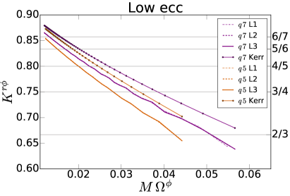
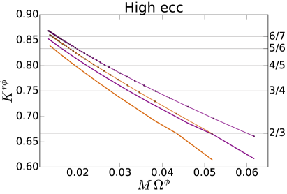
Figure 6: Precession rates $K^{r\phi}$ as a function of $M\Omega^{\phi}$ extracted from our equatorial simulations (thick solid, dashed, and dotted lines) and as predicted for a Kerr black hole of mass $M_{\rm Kerr}=m_{1}$ and the same eccentricity evolution (thin lines with symbols). We plot multiple resolutions for our simulations as indicated. Left: Precession of our low-eccentricity simulations. Right: Precession of our high-eccentricity simulations.

We plot our extracted precession rates $K^{r\phi}_{i}$ along with the geodesic predictions as functions of azimuthal frequency $M\Omega^{\phi}_{i}$ in figure 6. Several numerical resolutions are plotted, and we find agreement in our precession rates across resolutions. In addition, it is apparent that the finite mass corrections increase the magnitude of general relativistic precession, by decreasing $\Omega^{r}$ as compared to $\Omega^{\phi}$. Higher eccentricities also enhance the precession rate. Figure 6 enables identification of $r$-$\phi$ resonances, which are marked with horizontal lines. Our binaries plunge before the high-order $r$-$\phi$ resonances which are expected to generate resonant kicks. Thus, although the analytical results of [91] indicate these kinds of resonant kicks could be promising at mass ratios comparable to ours, we see that in reality the rate of inspiral is too high and significantly higher mass ratios are required to access the relevant resonances.

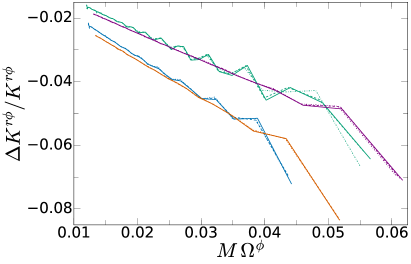
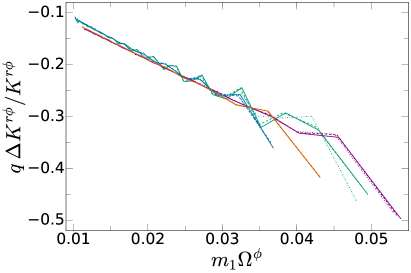
Figure 7: Comparison between the precession rates for our equatorial binary inspirals and Kerr geodesic theory. Specifically, we plot the differences $\Delta K^{r\phi}$ between the numerical extraction and geodesic prediction for the $r$-$\phi$ frequency ratio, divided by the numerical $K^{r\phi}$.

In the left panel of figure 7 we plot the relative difference between the numerical precession rates and geodesic predictions, $\Delta K^{r\phi}_{i}=K^{r\phi}_{{\rm Numeric,}i}-K^{r\phi}_{{\rm Kerr,}i}$, normalized by the numerical $K^{r\phi}_{i}$. We see that the geodesic prediction captures the precession rate well for our binaries, up to corrections of less than ten percent. As expected, the $q=7$ simulations are closer to the geodesic predictions than the $q=5$ simulations. Inspecting each mass ratio separately, we see that doubling the eccentricity has less than a percent impact on the relative differences.

Finally, we use our simulations to extract the $O(1/q)$ corrections to the geodesic precession rate, i.e. the leading conservative SF correction to $K^{r\phi}$. In the right panel of figure 7, we rescale the relative differences by $q$, and plot our results against $m_{1}\Omega^{\phi}_{i}$. This guarantees that we are expanding our results around the same test mass limit in all cases. Remarkably, we see that after this rescaling the $q=5$ and $q=7$ curves are nearly identical in both the high-eccentricity and low-eccentricity cases. This implies several things. First, that the higher order SF effects must be quite small, since a priori an $O(1/q^{2})$ correction would generate a similar split in the rescaled $q=5$ and $q=7$ curves as seen in the left panel of figure 7. Next, it must be true that the spin-dependence of the $O(1/q)$ SF correction is almost entirely captured by the prefactor, which is normalized out in each case. Finally, comparing the high- and low-eccentricity cases to each other, we see the same limited dependence on eccentricity as discussed for the left hand panel.

All together, we conclude that the periastron precession rate takes the form

$$K^{r\phi}(m_{1}\Omega^{\phi})=K^{r\phi}_{\rm Kerr}(m_{1}\Omega^{\phi})\left[1+\frac{1}{q}\Delta K^{r\phi}_{\rm SF}+O\left(\frac{1}{q^{2}}\right)\right]\,.$$ (19)

where $\Delta K^{r\phi}_{\rm SF}$ is nearly independent of spin and eccentricity at modestly large spins and low eccentricities, and the further $O(1/q^{2})$ terms are numerically small.

5 Inclined binaries

In this section, we extract the frequencies of motion for our eccentric, inclined simulations. In these cases, precession of the orbital plane and the black hole spin introduces a non-trivial dependence between all three of the characteristic frequencies. This complicates our procedure, but we are able to cleanly extract $K^{r\theta}$ and compare to Kerr geodesics. We find that our binaries pass through low order resonances in $r$-$\theta$ motion, and we investigate the fluxes of energy and angular momentum from our simulations to search for the imprint of these resonances.

5.1 Definition of frequencies

For inclined runs, there are two periodic modulations which both imprint themselves on the dynamics, cf. (3) and (4). When choosing averaging-periods, we cannot honour both periodicities simultaneously. Empirically, we find that windows over the radial rather than polar periods yield smoother frequencies. For instance, $\Omega$ varies much more strongly between periastron and apastron than for different values of $\theta$. These findings depend on the eccentricities considered here: we expect that if eccentricity were reduced at fixed inclination, eventually the polar oscillations would become more important than the radial oscillations.

The radial motion couples to the polar motion through spin-orbit coupling via terms proportional to $\hat{\bm{\chi}}_{1}\cdot\hat{\bm{r}}=\cos\theta$, which results in a $\cos\theta$-dependent modulation to the envelopes of $\Omega(t)$ and $r(t)$. This introduces some oscillation to both $\Omega^{r}$ defined in (16) and especially to the eccentricity $e$ (14). Nevertheless these effects are relatively small compared to those which would be introduced by choice of a different window for the $\Omega^{r}$ computation, and we continue to use the same relation as in the equatorial case: $\Omega^{r}$ is the reciprocal of the periods between maxima of the orbital frequency $\Omega(t)$, (16).

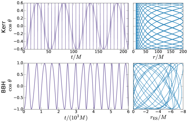
Figure 8: Plot of $\cos\theta$ versus $t$ (left) and $r$ (right) for a Kerr geodesic with semilatus rectum $p=20M$, eccentricity $e=0.9$, $i=36^{\circ}$, and spin parameter $\chi=0.9$ (top), compared with our high mass ratio and eccentricity $i=80^{\circ}$ BBH simulation (bottom). In the BBH case we use the envelope subtracted separation $r_{\rm ES}$, computed as described in section 3. Note in particular the strong dependence of $\partial_{r}\cos\theta$ upon $r$, most obviously visible in the Kerr phase plot. This strongly modulates the polar motion in time, resulting in the beating effect visible in both time series plots. This effect necessitates a more complex frequency-extraction strategy than taking simple peak-to-peak periods of the polar motion.

We now turn to the polar frequency $\Omega^{\theta}$, which we would like to define in terms of the binary black hole system’s polar motion $\theta(t)$. This angle $\theta(t)$ shows clear modulations due to the interdependence of the radial and polar motion: roughly, $\theta(t)$ varies most quickly near periastron. While the resultant modulations to $\theta(t)$ are most pronounced for highly eccentric orbits such as the Kerr geodesic shown in the upper panel of figure 8, they are still visible by eye at the eccentricities accessible to numerical simulations (cf. the lower panel of figure 8). A straightforward definition of polar frequency based on extrema of $\theta(t)$, while satisfactory for conservative orbits once averaged over infinite polar cycles, suffers from substantial interval-to-interval variations during a simulation, depending on the radial phase at successive $\theta(t)$ extrema.

The most obvious way to account for the dominant dependence on separation is to measure the polar frequency over intervals that begin and end at fixed radial phase. While we do not have access to such a phase in general, any reasonable definition of one will attain a fixed value at periastron. We therefore employ the same periastron-to-periastron intervals as those we used to define $\Omega^{r}$ (16). As an additional advantage, this choice results in an $\Omega^{\theta}$ defined at the same midpoint times $\tilde{t}^{+}_{i}$ as the other frequencies, such that comparisons do not require an interpolation.

Because the radial and polar frequencies are distinct, the periastron-to-periastron intervals $[t^{+}_{i},t^{+}_{i+1}]$ do not correspond to an integer number of polar oscillations. To account for this we define a polar phase $\chi^{\theta}(t)$ through equation (6), and we define $\cos\theta_{\rm min}$ using the maximal envelope of $\cos\theta(t)$, interpolated to the time of interest.

The function $\chi^{\theta}(t)$ is made monotonic and continuous by suitable choice of quadrant when inverting $\cos\chi^{\theta}$ followed by suitable additions of multiples of $2\pi$. We then define

$$\Omega^{\theta}_{i}\equiv\frac{\chi^{\theta}(t^{+}_{i+1})-\chi^{\theta}(t^{+}_{i})}{t^{+}_{i+1}-t^{+}_{i}}.$$ (20)

In D we show that this definition applied to Kerr limits to the exact polar frequency, with sub-percent error over single-cycle windows.

Finally, the azimuthal frequency $\Omega^{\phi}$ presents the most difficulties. For inclined Kerr orbits, the averaged orbital frequency $\langle\Omega\rangle$ differs from the azimuthal frequency $\Omega^{\phi}$. One solution would be to define $\Omega^{\phi}$ in terms of some azimuthal angle $\phi$, in a similar manner as in (20). Such a definition is possible, but all our attempts have resulted in an $\Omega^{\phi}$ which either fails to converge properly for Kerr orbits or which oscillates unacceptably wildly for single-cycle windows. To appreciate the difficulty, note for example that the “orbital plane” of the BBH simulation might reasonably be defined as the plane orthogonal either to the primary spin vector $\bm{\chi}_{1}$ or to the total angular momentum vector ${\bm{J}}$. Both choices recover the desired limit for $q\to\infty$, but are different planes at finite $q$.

On the other hand $\langle\Omega\rangle$ does furnish a fairly smooth frequency which is itself of some dynamical interest. We therefore report $\langle\Omega\rangle$ computed via (12) for the inclined orbits as well.

5.2 Precession rates

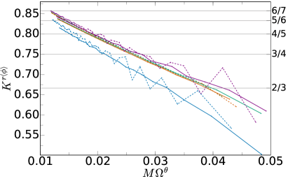
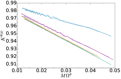
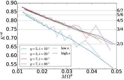
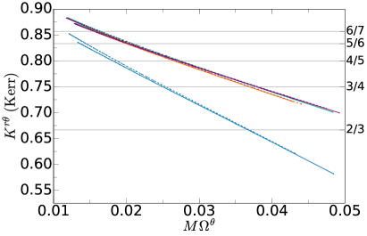
Figure 9: Precession rates for our inclined runs at highest resolution (L3). Resonant precession rates are highlighted with solid horizontal bars. The bottom right plot shows the Kerr $K^{r\theta}$, to be compared to the BBH data at the bottom left.

From the frequencies $\Omega^{r}$, $\Omega^{\theta}$ and $\langle\Omega\rangle$ we compute precession rates as frequency ratios $K^{ab}=\Omega^{a}/\Omega^{b}$. The results are shown in figure 9. As in section 4, we plot against a frequency, $M\Omega^{\theta}$, in order to mitigate any gauge effects. Since we cannot cleanly extract $\Omega^{\phi}$, we plot the ratios $K^{r\langle\phi\rangle}\equiv\Omega^{r}/\langle\Omega\rangle$ and $K^{\theta\langle\phi\rangle}\equiv\Omega^{\theta}/\langle\Omega\rangle$ in addition to $K^{r\theta}$. We do not have analytic predictions for the ratios involving $\langle\Omega\rangle$, but we can see some general trends. As the binary sweeps to higher frequencies, periastron precession becomes stronger as $\Omega^{r}$ lags further behind the other frequencies. Comparing the higher eccentricity to the lower eccentricity simulations at fixed $\Omega^{\theta}$, we see that $K^{ab}$ is smaller in the higher eccentricity cases. This is most apparent early in the inspirals (smaller $\Omega^{\theta}$), when there is a larger difference in $e$ between the cases; for all the $K^{ab}$, the solid lines lie at smaller values than the dashed, although the differences are small. This is true also for the Kerr predictions (bottom right of figure 9).

There is no clear effect of inclination on the precession rates $K^{r\theta}$ and $K^{r\langle\phi\rangle}$, except for $i=80^{\circ}$, where they are systematically smaller, i.e. periastron advance is more pronounced. Meanwhile, the effect of increasing inclination on $K^{\theta\langle\phi\rangle}$ is clearly visible: at higher inclinations, $\langle\Omega\rangle$ becomes more and more nearly equal to $\Omega^{\theta}$, and so their ratio approaches unity as we approach polar orbits.

Figure 9 shows large oscillations in the extracted precession rates $K^{r\theta}$ and $K^{r\langle\phi\rangle}$ for the simulations q7_i40_low-e and q7_i80_low-e. These oscillations can be traced to distinct features in the separation $r(t)$ for these two simulations. Compared to the other simulations considered here, $r(t)$ shows extra modulations for these two cases. We discuss this in more detail in D. We presently do not understand the origin of these additional features, nor the reason why they only appear in the simulations q7_i40_low-e and q7_i80_low-e. All $q=7$ simulations were run with identical source-code revision and configuration files.

Figure 10 illustrates the relative differences between the geodesic predictions and our numerical precession rates. We focus on $K^{r\theta}$, which we can compare to analytic theory. The top left panel of figure 10 shows the $q=5$ data, where we find no discernible difference between the inclinations $i=10^{\circ}$ and $i=20^{\circ}$. Further, as in the case of the equatorial inspirals, the difference between low eccentricity and high eccentricity is mild. The top right panel shows the high eccentricity case for the $q=7$ inspirals, and again we see only a mild dependence on the inclination, although it is discernible. The low $e$ runs for $q=7$, unfortunately, are dominated by the large modulations mentioned above and do not add any further insights.

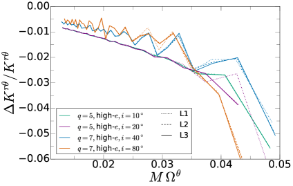
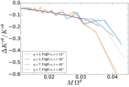
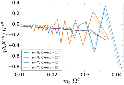
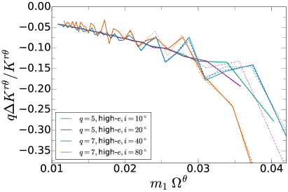
Figure 10: Top: Comparison of the numerical extraction of $K^{r\theta}(M\Omega_{\theta})$ to geodesic theory, for each of $q=5$ and $q=7$ (higher eccentricity simulations only). The frequencies for the low eccentricity $q=7$ simulations display large modulations, as can be seen in Fig. 9. Bottom: Plot of $\Delta K^{r\theta}/K^{r\theta}$ rescaled by $q$ and plotted against $m_{1}\Omega_{\theta}$ for each simulation. The left panel features the lower eccentricity simulations, and the right panel features the higher eccentricity simulations.

The lower panels of figure 10 plot the rescaled residual differences, with the lower eccentricity inspirals on the left and the higher eccentricities on the right. As seen before in figure 7, the fact that all the lines are nearly on top of each other indicates that the $O(1/q^{2})$ corrections are unexpectedly small, cf. equation (19). Even in the case of the $q=7$, low eccentricity runs, we see that the midline of the large modulations agrees well with the $q=5$ scaled residuals. Thus, the curves here roughly give the leading SF conservative corrections to the $r$-$\theta$ precession rate. Further, we see that the inclination, spin, and eccentricity dependence of this correction is mostly captured by scaling out the geodesic results.

5.3 Resonances

The frequencies computed in section 5 can be immediately exploited to detect resonances. We focus on the lowest order $r$-$\theta$ resonances our simulations achieve, which are the 5:6, 4:5, 3:4 and 2:3 resonances. In particular, self-force calculations using PN models [64, 92] have highlighted the importance of the 2:3 resonance.

   
   

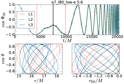
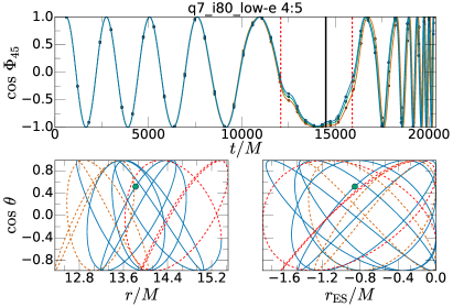
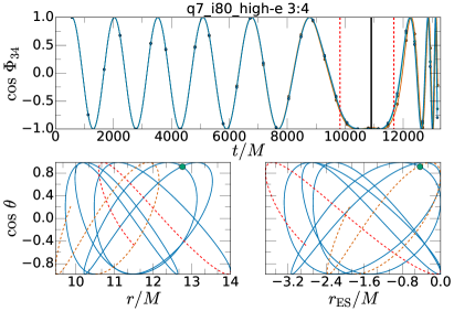
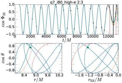
Figure 11: Pictorial analysis of $r$-$\theta$ resonances for four select resonances. For each example, a block of three graphs is presented, titled by the simulation and the resonance under consideration. Each block is organized as follows: Top graph: Resonant phase $\Phi_{kn}$ with vertical solid lines marking the resonance, vertical dashed lines bounding one radian in resonant phase in either direction, and black dots indicating midpoint times, $\tilde{t}^{+}_{i}$, cf. (13). The resonant phase $\Phi_{56}(t)$ in the top-left panel is plotted at three different numerical resolutions. Bottom left graph: Orbital trajectory during the resonance using two line-styles, solid lines represent one resonant cycle centered on the resonance (marked by a circle); dashed lines represent the remaining evolution within the resonant window. Bottom right graph: Trajectory with inspiral-motion removed, by using the envelope-subtracted radius $r_{\rm ES}$ (11).

The rough locations of the coordinate resonances can be identified from figure 9, where the relevant values of $K^{ab}$ are highlighted with horizontal lines. A somewhat better estimate can be obtained by solving the equation $k\Omega^{a}(t)-n\Omega^{b}(t)=0$ for integers $n,k$, where $n/k\leq 1$ gives the value of $K^{ab}$ at resonance. This avoids the noise in the quotient. Solving this equation gives us an estimate for the simulation time $t_{\rm res}$ at which a given resonance is encountered. Interpolating $\Omega^{\theta}$ onto this value gives an estimate of the corresponding polar frequency at resonance, $\Omega^{\theta}_{\rm res}$.

Following [116] we estimate the time spent on $r$-$\theta$ resonance using the following procedure. First, we construct a resonant phase $\Phi_{kn}(t)$

$$\Phi_{kn}(t)=\int_{t_{0}}^{t}\left[k\Omega^{\theta}(t^{\prime})-n\Omega^{r}(t^{\prime})\right]{\mathrm{d}}t^{\prime},$$ (21)

where the arbitrary reference time $t_{0}$ is chosen after initial transients of the numerical simulation. The significance of the phases $\Phi_{kn}$ arises from black hole perturbation theory, where the effect of the dissipative self-force upon the time derivative of some Kerr constant of motion $\mathcal{C}$ expands into Fourier modes $k$ and $n$ of the form

$$\frac{d\mathcal{C}}{dt}=\dot{\mathcal{C}}_{00}+\sum_{k=-\infty}^{\infty}\sum_{n=-\infty}^{\infty}\dot{\mathcal{C}}_{kn}e^{-i\Phi_{kn}(t)},\qquad n,k\neq 0.$$ (22)

The exponential terms in most cases average to zero since they oscillate rapidly compared to the overall evolution of $\mathcal{C}$. At resonance, however, the phase is constant and the respective term contributes secularly to $d\mathcal{C}/dt$.

A representative resonant phase for each order $k\!:\!n$ is shown in figure 11. Still following [116], we say the system is near resonance when $\Phi_{kn}$ differs from its resonant value by no more than 1 radian. This dephasing is indicated in figure 11 by the dashed vertical lines; our simulations satisfy this condition for durations of a few $1000M$. The duration $\Delta t_{\rm res}$ and frequency range $\Delta\Omega^{\theta}_{\rm res}$ during which our simulations stay on resonance can be readily determined from $\Phi_{kn}$. We estimate the number of radial and polar cycles spent on resonance by counting the number of relevant coordinate peaks within the resonance. These data are collected in table 2. Inspection of table 2 reveals that, with the 2:3 resonance excepted, our simulations remain on resonance long enough to trace out one or even two full resonant cycles. (cf. the coordinate plots in figure 11). On resonance, the $r$-$\theta$ motion of a geodesic is a Lissajous figure; figure 11 includes the corresponding plots for the full BBH simulation, highlighting that the character of the Lissajous figures are preserved.

Table 2: The $r$-$\theta$ resonances identified in our simulations. Given is the order of the resonance, the polar frequency $\Omega^{\theta}$ at resonance, the duration in terms of time $\Delta t_{\rm res}$ and polar frequency $\Delta\Omega^{\theta}_{\rm res}$, and the number of radial cycles $\mathcal{N}_{r}$ and polar cycles $\mathcal{N}_{\theta}$ during the resonance. For many of the 2:3 and some of the 6:7 resonances, the resonances were detected, but occurred too near plunge for their width to be measured; in those cases we report the frequency at resonance and mark the other columns n/a.

Run	Order	$M\Omega^{\theta}_{\rm res}$	$\Delta t_{\rm res}/M$	$M\Delta\Omega^{\theta}_{\rm res}$	$\mathcal{N}_{r}$	$\mathcal{N}_{\theta}$
q5_i10_low-e	6:7	0.0264	4540	0.00787	9	11
	5:6	0.0341	2921	0.00506	8	9
	4:5	0.0385	1737	0.00301	5	7
	3:4	0.0408	920.3	0.00159	4	5
q5_i20_low-e	6:7	0.0268	4646	0.00876	10	11
	5:6	0.0353	3026	0.00571	8	9
	4:5	0.0403	1792	0.00338	5	7
	3:4	0.0430	989.0	0.00187	4	5
q5_i10_high-e	6:7	0.0209	4713	0.0144	9	11
	5:6	0.0346	2982	0.00911	7	9
	4:5	0.0425	1757	0.00537	5	7
	3:4	0.0466	935.4	0.00286	4	5
	2:3	0.0531	n/a	n/a	n/a	n/a
q5_i20_high-e	6:7	0.0184	n/a	n/a	n/a	n/a
	5:6	0.0301	3088	0.00814	7	9
	4:5	0.0379	1821	0.00480	6	7
	3:4	0.0416	964.9	0.00254	4	5
q7_i40_low-e	6:7	0.0299	5048	0.00780	10	12
	5:6	0.0385	3253	0.00502	9	10
	4:5	0.0437	2076	0.00320	7	8
	3:4	0.0469	279.2	0.000431	1	2
	2:3	0.0515	n/a	n/a	n/a	n/a
q7_i80_low-e	5:6	0.0230	5569	0.00880	11	12
	4:5	0.0341	3817	0.00603	9	11
	3:4	0.0393	2182	0.00345	7	8
	2:3	0.0447	n/a	n/a	n/a	n/a
q7_i40_high-e	6:7	0.0224	5317	0.0124	11	12
	5:6	0.0360	3371	0.00784	8	10
	4:5	0.0435	1958	0.00456	7	8
	3:4	0.0475	954.9	0.00222	4	5
	2:3	0.0537	n/a	n/a	n/a	n/a
q7_i80_high-e	4:5	0.0311	3506	0.00975	8	10
	3:4	0.0421	1858	0.00517	6	7
	2:3	0.0469	815.3	0.00227	3	5

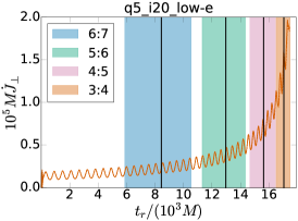
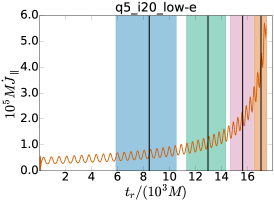
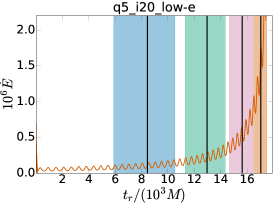
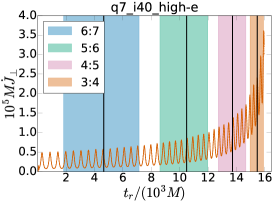
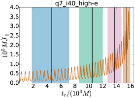
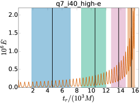
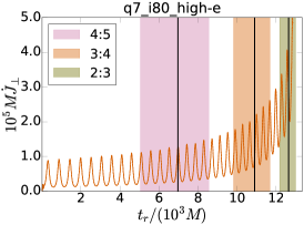
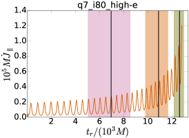
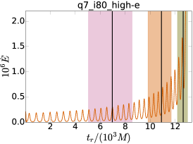
Figure 12: Gravitational wave fluxes during resonances. Each row of plots corresponds to one numerical simulation as indicated in the title of each panel. The columns correspond to three gravitational wave fluxes. Left: Angular momentum flux orthogonal to primary spin direction $\hat{\bm{\chi}}(t)$. Middle: Angular momentum flux tangential to $\hat{\bm{\chi}}(t)$. Right: Energy flux. Resonances are indicated by the shaded areas. The fluxes are shown at three resolutions, with differing linestyles; on the scale of the plot, however, these are indistinguishable in the plots except close to merger.

As table 2 and figure 11 indicate, our inspirals remain on resonance for one to two resonant cycles. This may lend some hope that secular accumulations from terms like those in (22) might be directly visible, leading to a noticeable change in the evolution of constants of motion ($\mathcal{E}$, $\mathcal{L}_{z}$, and $\mathcal{Q}$) during the inspiral. Returning to equation (22), we see that the impact of passage through a resonance is that a subset of the oscillatory contributions to $d\mathcal{C}/dt$ momentarily “freeze out”, with $\dot{\Phi}_{kn}$ passing through zero at the resonance for pairs $(k,n)$ commensurate with the resonance. Near the resonance, the phases of these contributions can be approximated by Taylor expanding $\Phi_{kn}$ around the time $t_{\rm res}$ when resonance is achieved (see e.g. [116])

$$\Phi_{kn}\approx\Phi_{kn}(t_{\rm res})+\frac{1}{2}(k\dot{\Omega}^{\theta}-n\dot{\Omega}^{r})|_{t_{\rm res}}(t-t_{\rm res})^{2}\,.$$ (23)

While the amplitude and sign of these resonant contributions to $d\mathcal{C}/dt$ depends on the coefficients $\dot{\mathcal{C}}_{kn}$ and the phase on resonance $\Phi_{kn}(t_{\rm res})$, these terms have a distinct time evolution: their contribution is approximately symmetric about $t_{\rm res}$, and they contribute over a time scale of approximately the resonant width $\Delta t_{\rm res}$. This characteristic time evolution is clearly seen in the plots of $\cos\Phi_{kn}$ in figure 11 around each resonant passage. Thus the simplest way to diagnose whether a resonant passage impacts the dynamics is to search for modulations of $d\mathcal{C}/dt$ with this behavior. Meanwhile, the time integral of these terms results in a jump in $\mathcal{C}$ which accumulates over a period approximately equal to $\Delta t_{\rm res}$. The detailed time evolution of these contributions involves Fresnel integrals (e.g. [92]), and is antisymmetric across the resonance.

To investigate the possibility of resonances affecting the orbital evolution, we compute the instantaneous gravitational wave energy flux $\dot{E}(t_{r})$ and the gravitational wave angular momentum fluxes $\dot{\bm{J}}(t_{r})$ as suitable products of spherical harmonic modes of the gravitational waveform [117] for all modes $l\leq 8$. These fluxes are given in terms of the retarded time

$$t_{r}=t-R-2M\ln\left(\frac{R}{2M}-1\right),$$ (24)

where $R$ is the gravitational wave extraction radius of each simulation ($\sim 500M$). For the angular momentum flux, we project parallel and orthogonal to the primary BH-spin direction $\hat{\bm{\chi}}(t)$,

$$\dot{J}_{||}(t_{r})=\dot{\bm{J}}(t_{r})\cdot\hat{\bm{\chi}}(t),$$ (25)

$$\dot{J}_{\perp}(t_{r})=\left|\dot{\bm{J}}(t_{r})-J_{||}(t_{r})\hat{\bm{\chi}}(t)\right|.$$ (26)

We use $\dot{J}_{||}$ as a proxy for the azimuthal angular momentum flux of the test body (corresponding to the constant of motion $\mu\mathcal{L}_{z}$), and $\dot{J}_{\perp}$ as a very rough proxy for the evolution of the square root of the Carter constant $\mu\sqrt{\mathcal{Q}}$.

In figure 12 we plot the energy- and angular momentum-fluxes for three simulations with the time-intervals on resonance indicated. Figure 12 shows short-period modulations due to eccentricity, with sharp spikes near each periastron passage. However, no additional modulations over the resonant timescales are discernible. We have also examined the angular momentum ${\bm{J}}$ and total energy $E$ by integrating the fluxes, and see no excess build-up or deficit over the resonant widths.

The amplitude of any changes that occur during resonance depends on the resonant phase and it is possible that all of our simulations have phases that make resonant effects undetectable. Unfortunately, the resonant phase cannot be easily changed in a numerical simulation while keeping all other parameters constant. Since it is unlikely that all resonances are encountered with unfavorable phases, we interpret the absence of detectable resonant modulations as evidence that the mass-ratios and eccentricities under consideration are not extreme enough to exhibit strong resonant effects.

In E we estimate quantitatively the strength of resonant effects by fitting a sufficiently-stiff function to peak-to-peak averages over the gravitational wave fluxes averaged roughly over the resonant timescale. Since the chosen function is too stiff to capture resonant-timescale effects, resonant accumulations should be visible as jumps in the residuals over that timescale. Using this method on the most extreme cases of the q7_i40_high-e and q7_i80_high-e runs we bound resonant effects upon these runs from above at less than the 0.4% level.

6 Conclusions

We have presented a suite of binary black hole simulations performed with the SpEC code that aim to explore the relation between BBH systems and generic Kerr geodesics. Our simulations are eccentric and explore both precessing and nonprecessing configurations. The simulations cover 30–60 radial passages and multiple precession cycles, and are performed at comparatively high mass-ratios of $q=5$ and $q=7$.

As a first step to understanding these fully generic binary inspirals, we developed methods for extracting the instantaneous, fundamental frequencies of motion while partially accounting for dissipative effects. In the case of equatorial inspirals, these are the frequencies of radial motion $\Omega^{r}$ and azimuthal motion $\Omega^{\phi}$ averaged over a radial orbit. Here the frequencies can be extracted most cleanly, since the interdependence of the polar and the radial motion does not come into play and does not produce frequency modulations. The ratio of these frequencies provides the rate of periastron advance and is a physically measurable quantity. We have compared the precession rate of our eccentric binaries to geodesic orbits in Kerr, and extracted the leading self-force correction to this rate. Our results show that second-order SF corrections to these rates is small, and that much of the dependence on eccentricity and black hole spin can be absorbed into the leading Kerr behavior.

In the case of our generic, precessing binaries, we can cleanly extract the fundamental frequencies of radial and polar motion, as well as the average orbital frequency $\left<\Omega\right>$. The fundamental azimuthal frequency $\Omega^{\phi}$ differs from $\left<\Omega\right>$ because motion in the orbital plane is a mixture of azimuthal and polar motions for precessing binaries. Unfortunately, it turns out that $\Omega^{\phi}$ is affected by interactions of the polar and radial motions to a large degree, cf. D. Nevertheless, we have extracted the ratios of radial, polar, and average orbital frequencies from our simulations, cf. figure 9. The ratio $K^{r\theta}=\Omega^{r}/\Omega^{\theta}$ can be predicted for Kerr geodesics, and in this case we have compared to analytic theory and extracted the SF corrections to our precession rates.

Finally, with our fully generic orbits we were able to identify low-order orbital resonances in the radial-polar motion, and show that our systems pass through resonances with $\Omega^{r}/\Omega^{\theta}=$ 5:6, 4:5, 3:4 and 2:3. Our simulations remain on resonance usually for more than one resonant cycle, and sometimes up to two resonant cycles. The $r$–$\theta$ resonances have been shown to have an impact on the adiabatic inspirals of extreme mass ratio systems[78, 63], and our study is the first to identify them in a numerical spacetime. However, at the mass ratios we have achieved we find no clear impact on the fluxes of energy and angular momentum of our systems (cf. figure 12).

In two of our low-eccentricity simulations, strong residual oscillations in the extracted frequencies dominate the comparison. These modulations arise from small but visible variations in the radial separation of the binary, persist at several resolutions, and will be the subject of future investigation.

In this study we have focused on the dynamics of the black holes themselves. In future studies we will examine the gravitational waveforms produced by these systems, and explore the extraction of the fundamental frequencies directly from the waveform. Waveforms from our equatorial and fully generic system will serve to test how detectable these binaries are using current quasi-circular and eccentric waveform models, as well as help develop those models further. Waveforms from these binaries can also elucidate what constraints can be placed on eccentricities in future gravitational wave detections.

Future work will include extending our suite of simulations to higher mass ratios, and to cover a larger range of eccentricities and binary configurations. We will extract the redshift factor [118] from generic black hole binaries, which is analogous to the Lorentz factor of the black holes. With three frequencies and the Lorentz factor, we can imagine forming an explicit map between high mass ratio binaries and perturbed orbits in Kerr. Comparisons to post-Newtonian predictions for the frequencies of motion would supplement our SF-inspired comparisons to Kerr geodesics. In addition, SF predictions in for Kerr orbits are developing rapidly (e. g. [69, 119]), which will allow for a quantitative comparison to analytic approximations, as well as an extraction of higher-order SF effects.

In previous studies of circular orbits, it was suggested that re-expanding geodesic predictions about the symmetric mass ratio $\nu=m_{1}m_{2}/M^{2}$ and as functions of $M\Omega^{\phi}$ would provide for faster convergence to the numerical results [71, 73]. With a SF prediction for the precession rates in our equatorial and generic binaries, we will be able test this promising idea in a new regime.

Appendix A The Kerr metric

The Kerr metric expressed in Boyer-Lindquist coordinates $x^{\mu}=(t,r,\theta,\phi)$ is given by

$$ds^{2} = -\left(1-\frac{2Mr}{\rho^{2}}\right)dt^{2}-\frac{4Mar\sin^{2}\theta}{\rho^{2}}dtd\phi+\frac{\rho^{2}}{\Delta}dr^{2}+\rho^{2}d\theta^{2}$$ (27)

$$+\frac{\sin^{2}\theta}{\rho^{2}}\left[(r^{2}+a^{2})^{2}-a^{2}\Delta\sin^{2}\theta\right]d\phi^{2}\,.$$

where $\rho^{2}=r^{2}+a^{2}\cos\theta$, $\Delta=r^{2}-2Mr+a^{2}$, and $M=M_{\rm Kerr}$ in this appendix only.

The equations of motion for a test particle are given by (2)–(4), and the explicit forms of the potentials are (see e.g. [84])

$$R(r) = \left[\mathcal{E}(r^{2}+a^{2})-a\mathcal{L}_{z}\right]^{2}-\Delta\left[(a\mathcal{E}-\mathcal{L}_{z})^{2}+r^{2}+\mathcal{Q}\right]\,,$$ (28)

$$\Theta(\theta) = \mathcal{Q}-\cos^{2}\theta\left[a^{2}(1-\mathcal{E}^{2})+\mathcal{L}_{z}^{2}\csc^{2}\theta\right]\,,$$ (29)

and

$$T_{r}(r)=\frac{r^{2}+a^{2}}{\Delta}\left[\mathcal{E}(r^{2}+a^{2})-a\mathcal{L}_{z}\right]\,,\qquad T_{\theta}(\theta)=-a^{2}\mathcal{E}\sin^{2}\theta\,,$$ (30)

$$\Phi_{r}(r)=\frac{a}{\Delta}\left[\mathcal{E}(r^{2}+a^{2})-a\mathcal{L}_{z}\right]\,, \Phi_{\theta}(\theta)=\mathcal{L}_{z}\csc^{2}\theta\,.$$ (31)

The radial equation can be converted into one for the radial phase $\chi^{r}$, and the polar equation into one for the phase $\chi^{\theta}$ in a straightforward manner using (5) and (6). It is these equations that we integrate to generate Kerr orbits of fixed $(p,e,i)$ to test our frequency extraction methods.

Appendix B Envelope subtraction method in the slow time approximation

In this appendix we demonstrate the utility of the envelope subtraction method discussed in section 3. The goal of this method is to locate the successive maxima $t^{+}_{i}$ or minima $t^{-}_{i}$ of the underlying motion of an oscillator with slowly varying parameters, and use them to calculate the frequency of oscillation. The variation of the amplitude and midline of the underlying oscillation shifts the position of the extrema from where they would be in the absence of the slow changes. We quantify the utility of the envelope subtraction method in removing these shifts by analyzing a toy model which captures some of the behavior of $\Omega(t)$ in our equatorial inspirals.

To model the orbital frequency, consider a function $f(\tilde{t},t)$ of a fast time $t$ and a slow time $\tilde{t}=\epsilon t$, with $\epsilon\ll 1$ giving the ratio of inspiral to orbital time scales. In order to represent an underlying oscillation at a single fixed frequency $\omega$, we assume that $f$ is periodic with period $P=2\pi/\omega$ in the fast time,

$$f(\tilde{t},t+P)=f(\tilde{t},t).$$ (32)

Since $\tilde{t}=\epsilon t$, after a period $f$ does not return to precisely the same value, but is modified by the advance of the slow time variable.

The maxima of the underlying oscillation are the extrema of $f$ in the limit $\epsilon\to 0$. For simplicity we phrase the discussion in terms of maxima; the procedure is identical for minima. For nonzero $\epsilon$, we find the maxima $t_{i}$ by solving

$$\frac{df}{dt}=\partial_{t}f+\epsilon\partial_{\tilde{t}}f=0$$ (33)

order by order in $\epsilon$, under the ansatz

$$t_{i}=t^{(0)}_{i}+\epsilon t^{(1)}_{i}+O(\epsilon^{2})\,.$$ (34)

At leading order, we have as expected

$$\left.\partial_{t}f\right|_{t^{(0)}_{i}}=0\,,$$ (35)

which shows that $t^{(0)}_{i}$ are the maxima of the underlying oscillation. We seek $t^{(0)}_{i}$, but we have only access to $t_{i}$ when analyzing $f$. From equation (34) we see that the naive maxima $t_{i}$ incur an error $O(\epsilon)$.

Returning to equation (33), we Taylor expand all quantities around $t=t_{i}^{(0)}$ to find at the next order that

$$t_{i}^{(1)}=-\left.\frac{\partial_{\tilde{t}}f}{\partial_{t}^{2}f}\right|_{t_{i}^{(0)}}\,.$$ (36)

This provides the leading error on our estimation of the maxima. We can iterate this procedure to compute higher order errors, but it turns out we can instead identify a different function, the envelope subtracted $f$, whose maxima are closer to $t_{i}^{(0)}$.

We first fit a function through the maxima $t_{i}$ (in practice a spline of at least cubic order). This envelope $f^{+}(\tilde{t})$ describes the slow time variation passing from maximum to maximum, meaning that $f^{+}(\tilde{t})=f(\tilde{t},t_{i}^{+})$. By Taylor expansion about $t_{i}^{(0)}$ we have

$$f^{+}(\tilde{t})=f(\tilde{t},t_{i}^{(0)})-\epsilon^{2}\left.\frac{(\partial_{\tilde{t}}f)^{2}}{2\partial_{t}^{2}f}\right|_{t_{i}^{(0)},\tilde{t}}+O(\epsilon^{3})\,,$$ (37)

where we have simplified this function by recalling that $f(\tilde{t},t_{i}^{(0)}+nP)=f(\tilde{t},t^{(0)}_{i})$.

Next, we define the “envelope-subtracted” function

$$\hat{f}=f-f^{+}\,,$$ (38)

and seek its maxima. To motivate this definition, imagine we could seek the maxima of

$$f(\tilde{t},t)-f(\tilde{t},t^{(0)}_{i})\,,$$ (39)

which are given by the condition

$$\partial_{t}f(\tilde{t},t)-\epsilon[\partial_{\tilde{t}}f(\tilde{t},t)-\partial_{\tilde{t}}f(\tilde{t},t^{(0)}_{i})]=0\,.$$ (40)

The solutions are in fact the desired maxima, $t=t_{i}^{(0)}$, but we cannot formulate this ideal subtraction because we cannot identify $f(\tilde{t},t^{(0)}_{i})$. Fortunately, $\hat{f}$ is is equal to $f(\tilde{t},t^{(0)}_{i})$ up to $O(\epsilon^{2})$, and so we search for the maxima of (38).

We find that the maxima of $\hat{f}$, which we denote $\hat{t}_{i}$, are

$$\hat{t}_{i}=t_{i}^{(0)}+\epsilon^{3}\left.\delta t_{i}\right|_{t_{i}^{(0)}}+O(\epsilon^{4})\,,$$ (41)

$$\delta t_{i}\equiv-\frac{(\partial_{\tilde{t}}f)^{2}}{\partial_{t}^{2}f}\partial_{\tilde{t}}\left(\ln\partial_{\tilde{t}}f-\frac{1}{2}\ln\partial_{t}^{2}f\right)\,.$$ (42)

The error in $\hat{t}_{i}$ (relative to the desired maxima $t_{i}^{(0)}$) is $O(\epsilon^{3})$, i.e. envelope substraction has resulted in an improvement by two powers of $\epsilon$.

When we actually compute the frequencies, the error is even lower. We have

$$\hat{t}_{i+1}-\hat{t}_{i} = t^{(0)}_{i+1}-t^{(0)}_{i}+\epsilon^{3}(\delta t_{i+1}-\delta t_{i})+O(\epsilon^{4})$$ (43)

$$= P+\epsilon^{3}[\delta t(t_{i}^{(0)}+P,\epsilon t_{i}^{(0)}+\epsilon P)-\delta t_{i}]+O(\epsilon^{4})$$

$$= P+\epsilon^{4}P\partial_{\tilde{t}}(\delta t)|_{t^{(0)}_{i}}+O(\epsilon^{5})$$

where we have used the periodicity of $f$ in the variable $t$ and expanded the slow time function at $t_{i+1}$ about $t_{i}$. The above expressions are understood to be evaluated at $t_{i}^{(0)}$. The differencing at the extrema leads to an error $O(\epsilon^{4})$ due to another cancellation of the leading order correction to the period, due to slow evolution of the function and its envelope from maximum to maximum. Without the envelope subtraction procedure, the differencing at successive peaks results in an $O(\epsilon^{2})$ error in the extraction of the period.

Appendix C Evolution of eccentricity and semi-major axis

In this appendix we collect the relevant results of [6, 115] for the evolution of the eccentricity of a binary at lowest PN order. In this case, we consider a binary in an eccentric, Newtonian orbit, which sources gravitational wave emission through the quadrupole formula. The resulting orbit-averaged emission of energy and angular momentum changes the Newtonian parameters over the course of the slow inspiral. Peters [115] provides differential equations for orbit-averaged changes to the semi-major axis and eccentricity, $da/dt$ and $de/dt$, in terms of $(a,e)$. These can be solved numerically given initial conditions $(a_{0},e_{0})$, or combined and integrated to give an analytic expression for $a(e)$,

$$a=c_{0}\frac{e^{12/19}}{1-e^{2}}\left(1+\frac{121}{304}e^{2}\right)^{870/2299}\,,$$ (44)

where the integration constant $c_{0}$ is determined by $(a_{0},e_{0})$. In order to re-express this equation as the evolution of eccentricity with averaged orbital frequency $\langle\Omega\rangle$, we recall Kepler’s law for Newtonian orbits, $m=\langle\Omega\rangle^{2}a^{3}$. We can then write

$$\frac{\langle\Omega\rangle}{\langle\Omega\rangle_{0}}=\left(\frac{e}{e_{0}}\right)^{-18/19}\left(\frac{1-e_{0}^{2}}{1-e^{2}}\right)^{-3/2}\left(\frac{1+\frac{121}{304}e^{2}}{1+\frac{121}{304}e_{0}^{2}}\right)^{-1305/2299}.$$ (45)

Given and initial eccentricity and starting frequency, this formula provides us with an curve describing $e(\langle\Omega\rangle)$. We compare this leading post-Newtonian result to our numerical simulations in figure 5.

Appendix D Validation of frequency extraction methods

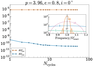
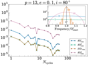
Figure 13: Performance of frequency extraction for Kerr-geodesics. Shown are the RMS differences $\delta\Omega^{a}_{\rm rms}=||\Omega^{a}-\Omega^{a}_{\mathrm{exact}}||/\Omega^{a}_{\mathrm{exact}}$, where $\Omega^{a}$ is computed from the geodesic trajectory with the same techniques we employ for our BBH analysis, and $\Omega^{a}_{\mathrm{exact}}$ is the exact frequency of the Kerr geodesic, for which we also show $\Omega^{\theta}$ and $\left<\Omega\right>$. We repeat the frequency-extraction using intervals covering $N_{\rm cycles}$ radial oscillation periods, and plot the resulting $\delta\Omega^{a}_{\mathrm{rms}}$ as a function of $N_{\rm cycles}$ The insets show absolute values of FFTs on $\Omega(t)$ computed over widths of $1,3,10$ and $50$ radial cycles, with the solid black line highlighting $\Omega^{r}_{\mathrm{exact}}$. Even at 50 cycles the peaks remain unacceptably broad.

This appendix assesses the accuracy of our frequency extraction techniques by application to Kerr geodesics, whose fundamental frequencies are known analytically. We compute one equatorial Kerr geodesic (eccentricity $e=0.8$, semilatus rectum $p=3.96M$), and one inclined Kerr geodesic (inclination $i=80^{\circ}$, $e=0.1$, $p=13M$). The geodesics are integrated with high precision by an ODE integrator, but we output only a discrete time series with spacing similar to that of the BBH simulations of our main analysis. We then apply the frequency extraction techniques described in sections 4 and 5 to the discrete time series. In addition to computing frequencies over $N_{\rm cycles}=1$ radial cycle, we also compute these frequencies over $N_{\rm cycles}\geq 2$ radial cycles by changing “$i+1$” to “$i+N_{\rm cycles}$” in equations (12) and (16). For each value of $N_{\rm cycles}$ we compute the relative difference $\delta\Omega^{a}_{i}=(\Omega^{a}_{i}-\Omega^{a}_{\mathrm{exact}})/\Omega^{a}_{\mathrm{exact}}$, and and its root-mean-square

$$\delta\Omega^{a}_{\rm rms}\equiv\left(\frac{1}{N}\sum_{i}^{N}(\delta\Omega^{a}_{i})^{2}\right)^{1/2}.$$ (46)

Here, $N$ is the number of elements $\delta\Omega^{a}_{i}$ for the current value of $N_{\rm cycles}$.

The left panel of figure 13 shows the results for the equatorial geodesic. Equatorial geodesics are strictly periodic and equations (12) and (16) should recover the exact frequencies, up to the numerical accuracy of our extraction techniques. Indeed, $\delta\Omega^{\phi}_{\rm rms}$ in the left panel is dominated by our numerical procedure to compute $\Omega$, which involves a fourth-order spline interpolant in the construction of $\dot{\bm{r}}$, and $\delta\Omega^{\phi}_{\rm rms}$ decreases as the fourth power of the time-sampling of the geodesic data. The accuracy of the extraction of $\Omega^{r}$ is limited by the accuracy $\sim 10^{-6}M_{\rm Kerr}$ with which our procedure determines the times $t_{i}^{+}$ of the maxima of $\Omega(t)$. Our extraction errors for the equatorial orbits are several orders of magnitude smaller than the systematic errors that arise due to genuine multi-periodicity for inclined orbits.

We now turn to the analysis of the inclined geodesic, which is presented in the right panel of figure 13. The radial frequency $\Omega^{r}$ is recovered to an accuracy better than $1\%$ when $N_{\rm cycles}=1$. The polar frequency $\Omega^{\theta}$ and the average orbital frequency $\left<\Omega\right>$ are recovered to nearly $0.1\%$. We also illustrate extraction of the azimuthal frequency $\Omega^{\phi}$. To extract $\Omega^{\phi}$, we begin by defining an “in-plane” separation vector ${\bm{\rho}}={\bm{r}}-({\bm{r}}\cdot\hat{\bm{\chi}})\hat{\bm{\chi}}$, where $\hat{\bm{\chi}}$ is the direction of the black hole angular momentum. We compute an instantaneous azimuthal frequency by

$$\Omega^{\rho}(t)=\frac{{\bm{\rho}}\times\dot{\bm{\rho}}}{\bm{\rho}^{2}}$$ (47)

and obtain the averaged azimuthal frequency $\Omega^{\phi}$ by evaluating the right-hand-side of (12), substituting $\Omega^{\rho}(t)$ for $\Omega(t)$. We recover $\Omega^{\phi}$ with a fractional accuracy of about $10\%$ (for $N_{\rm cycles}=1$).

The errors $\delta\Omega^{a}_{\rm rms}$ for the inclined geodesic stem from the interaction of the radial and polar motion. Simply put, subsequent periastron passages occur at different values of $\theta$. As the extraction interval is lengthened (larger $N_{\rm cycles}$), this dependence is averaged out over a longer time-intervals, and $\delta\Omega^{a}_{\rm rms}$ fall $\propto 1/N_{\rm cycles}$. The magnitudes of $\delta\Omega^{a}_{\rm rms}$ for each frequency depend on how important the interactions between radial and polar motion are for that particular frequency. The chosen geodesic has high inclination $i=80^{\circ}$ and fairly small eccentricity $e=0.1$; while the radial motion provides the dominant modulations (and our choice to average over radial periods $[t_{i}^{+},t_{i+N_{\rm cycles}}^{+}]$ is appropriate), the considered geodesic emphasizes the impact of the polar motion. As this example demonstrates, $\Omega^{\phi}$ is most susceptible to modulations, a finding that we confirm for the BBH systems, and which provides the basis for our preference of $\left<\Omega\right>$ over $\Omega^{\phi}$.

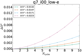
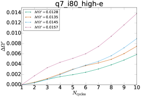
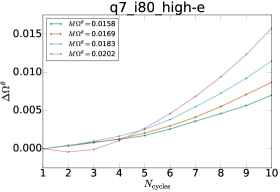
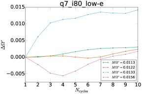
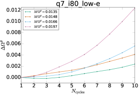
Figure 14: Robustness of frequency-extraction under change of width of extraction window. We extract frequencies using windows of $N_{\rm cycles}$ radial cycles, and plot the relative deviation from the same frequencies extracted at $N_{\rm cycles}=1$. Different panels represent different simulations, and the curves within each panel correspond to different times $\tilde{t}^{+}_{i}$. For the equatorial simulations (top panels), the radial and azimuthal frequencies are shown, whereas for the inclined simulations (middle and bottom panels), the radial and polar frequencies are plotted.

The insets in figure 13 illustrate frequency-extraction with more conventional Fourier techniques, in the form of periodograms computed from Fourier transforms of Hann-windowed samples of $\Omega(t)$ over window-sizes of $N_{\mathrm{cycles}}=1,\,3,\ 10$, and $50$ radial passages. For sufficiently long window-sizes, the periodograms do converge to the exact Kerr-frequency. However, at window sizes practical for the inspiral rate of our BBH simulations ($N_{\rm cycles}=1,3$), periodograms do not yield any useful information, and even when using 50 radial cycles, the achieved accuracy is only $\sim 1\%$.

Figure 14 examines the impact of the length of the extraction intervals (parameterized by $N_{\rm cycles}$) for our BBH simulations. We extract frequencies $\Omega^{a}_{N}$ computed over intervals of length $N=N_{\rm cycles}$, which we associate with the midpoint times $\tilde{t}^{+}_{i,N}=(t_{i}^{+}+t_{i+N}^{+})/2$. We interpolate the time series $\Omega^{a}_{N}$ onto the mid-times $\tilde{t}^{+}_{i}$, and compute the relative difference from the $N_{\mathrm{cycles}}=1$ case,

$$\Delta\Omega_{N}^{a}=\frac{\Omega^{a}_{N}-\Omega^{a}_{1}}{\Omega^{a}_{1}},$$ (48)

where the subscript denotes the value of $N_{\rm cycles}$ over which the frequency is computed. Because the characteristic frequencies increase during the inspiral, we report $\Delta\Omega_{N}^{a}$ at select values of $\Omega^{a}$, rather than the RMS error across the whole series.

In all cases we find that $\Delta\Omega^{a}$ increases with $N_{\rm cycles}$, with the largest $\Delta\Omega^{a}$ closer to merger (i.e. at larger $\tilde{t}^{+}_{i}$). For equatorial orbits our frequency extraction is very precise, and so $N_{\rm cycles}=1$ will ensure the least impact by errors arising from dissipative inspiral. For precessing orbits, there are two competing effects: First, with increasing $N_{\rm cycles}$, the impact of cycle-to-cycle modulations diminishes, leading to extracted sequences $\Omega^{a}_{i}$ that show less variations between neighboring extrema $i$. Second, increasing $N_{\rm cycles}$ leads to larger systematic biases of the extracted frequencies $\Omega^{a}_{i}$, cf. figure 14. To avoid contamination by such systematic biases, we choose $N_{\rm cycles}=1$ throughout, accepting possibly larger variations of the extracted frequencies.

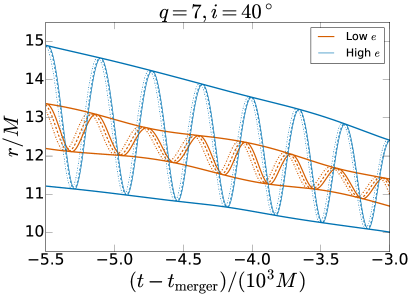
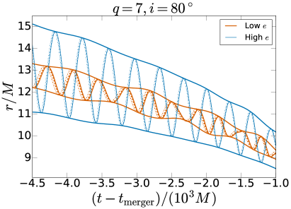
Figure 15: Separation $r(t)$ for the two “ill-behaved” low-eccentricity simulations, zoomed in to show the aperiodic behaviour. Also plotted are the envelopes of $r(t)$ to more clearly show the strong modulations in the low-eccentricity simulations. Three different numerical resolutions are plotted as different linestyles; the behaviour is convergent and mostly identical across resolutions.

Some of our simulations result in extracted frequencies that are noticably more erratic than the rest of the runs. This effect is most striking for the low-eccentricity highly-inclined orbits, cf. lower left panel of figure 9. These simulations are ill-behaved throughout our study, yielding far less smooth precession rate curves than their counterparts (cf. figure 9). Study of the separation $r(t)$ for these simulations (cf. figure 2) reveals unusually strong aperiodic features in the trajectories, which persists across our different numerical resolutions, which we show in figure 15. Curiously, the aperiodicity is far less dramatic at higher eccentricities, and indeed worsens during approach to merger, where the eccentricity is lower. This may be a sign that for these particular parameter choices quasi-periodic effects are comparable to dissipative ones, and that therefore $N_{\mathrm{cycles}}=1$ (or any constant $N_{\mathrm{orbits}}$) is inappropriate here. Alternatively, this may be an effect of the damped-harmonic SpEC simulation gauge [98, 99, 100], whose behaviour is largely untested for dynamically generic orbits.

Appendix E Estimation of resonant accretion

To increase the sensitivity to potential resonant effects, we can average the fluxes $\dot{J}_{\perp}$, $\dot{J}_{\parallel}$ and $\dot{E}$ over $N$ radial oscillation periods, where we slide the averaging window to start at each maximum of the respective flux. From (22), we expect that non-resonant terms are averaged out by this procedure. Therefore, off-resonance, the averaged fluxes

$$\langle\dot{\mathcal{C}}\rangle\approx\dot{\mathcal{C}}_{00}$$ (49)

correspond to the $\dot{\mathcal{C}}_{00}$ term. When averaging over a time window smaller than the time on resonance, and when the window is centered on the resonance, we can approximate $\Phi_{kn}(t)\approx\Phi_{kn}(t_{\rm res})$ over the averaging window. Then (22) yields

$$\langle\dot{\mathcal{C}}\rangle\approx\dot{\mathcal{C}}_{00}+\dot{\mathcal{C}}_{kn}e^{-i\Phi_{kn}(t_{\rm res})}.$$ (50)

Therefore, during resonance, the averaged fluxes $\langle\dot{\mathcal{C}}\rangle$ should show a relative deviation with peak amplitude $\delta\dot{C}\sim\dot{\mathcal{C}}_{kn}e^{-\Phi_{kn}(t_{\rm res})}/\dot{\mathcal{C}}_{00}$ compared to orbits off-resonance.

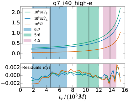
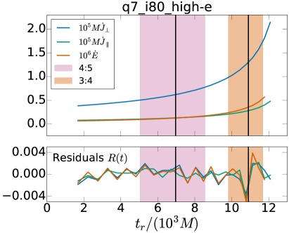
Figure 16: Gravitational wave fluxes averaged over $N=5$ radial oscillation periods for the runs q7_i40_high-e and q7_i80_high-e. The top panels show the actual data, and the lower panels the normalized residuals with respect to a fit that removes the overall inspiral trend, cf. (51).

The resulting averaged fluxes are shown in the top panel of figure 16 for two of our most extreme simulations, q7_i40_high-e and q7_i80_high-e. On the vertical scale of these plots, no variations of the fluxes are discernible between on- and off-resonance. To sharpen our bound, we remove the overall inspiral component of the fluxes through a fit to a function $f_{\rm fit}(t)=A_{0}(A_{1}-t)^{A_{2}}+A_{3}$. The functional form is chosen to capture the overall inspiral behavior, while not being able to capture intermediate variations that are expected on resonance. Therefore, we expect $f_{\rm fit}(t)\approx\dot{\mathcal{C}}_{00}$. The normalized residual

$$R(t)=\frac{\langle\dot{\mathcal{C}}\rangle-f_{\rm fit}}{\langle\dot{\mathcal{C}}\rangle}$$ (51)

should therefore vanish off-resonance. On-resonance, (50) suggests that (dropping terms of order unity) $R\sim\dot{\mathcal{C}}_{kn}e^{-i\Phi_{kn}(t_{\rm res})}/\dot{\mathcal{C}}_{00}$. As can be seen from the lower panels of figure 16, we find numerically $R\lesssim 0.004$. The short-period variations in $R$ in this figure are caused by the numerical accuracy with which we can extract periastron passages and perform the averaging. The overall smooth trend ($R$ is slightly negative at small $t$) indicates the quality with which our fitting function $f_{\rm fit}$ can capture the overall inspiral dynamics. Besides these two properties of $R(t)$, figure 16 does not show any systematic deviations at the highlighted resonances. Therefore, we conclude for these resonances that

$$\frac{\dot{\mathcal{C}}_{kn}e^{-i\Phi_{kn}(t_{\rm res})}}{\dot{\mathcal{C}}_{00}}\lesssim 0.004.$$ (52)

References

References

- [1] Abbott B P et al. (LIGO Scientific Collaboration, Virgo Collaboration) 2016 Phys. Rev. Lett. 116(6) 061102 (Preprint 1602.03837) URL http://link.aps.org/doi/10.1103/PhysRevLett.116.061102
- [2] Abbott B P et al. (LIGO Scientific Collaboration, Virgo Collaboration) 2016 Phys. Rev. D 93 122003 (Preprint 1602.03839)
- [3] Abbott B P et al. (LIGO Scientific Collaboration, Virgo Collaboration) 2016 Phys. Rev. Lett. 116 241103 (Preprint 1606.04855)
- [4] Cadonati L et al. (LIGO Scientific Collaboration, Virgo Collaboration) 2015 The LSC-Virgo white paper on gravitational wave searches and astrophysics URL https://dcc.ligo.org/LIGO-T1500055/public
- [5] Abbott B P et al. (Virgo, LIGO Scientific) 2016 Phys. Rev. X6 041015 (Preprint 1606.04856)
- [6] Peters P C and Mathews J 1963 Phys. Rev. 131 435 URL http://link.aps.org/abstract/PR/v131/p435
- [7] Khan S, Husa S, Hannam M, Ohme F, Pürrer M, Jiménez Forteza X and Bohé A 2016 Phys. Rev. D93 044007 (Preprint 1508.07253)
- [8] Taracchini A, Buonanno A, Pan Y, Hinderer T, Boyle M, Hemberger D A, Kidder L E, Lovelace G, Mroue A H, Pfeiffer H P, Scheel M A, Szilágyi B, Taylor N W and Zenginoglu A 2014 Phys. Rev. D 89 (R) 061502 (Preprint 1311.2544)
- [9] Hannam M, Schmidt P, Bohé A, Haegel L, Husa S et al. 2014 Phys. Rev. Lett. 113 151101 (Preprint 1308.3271)
- [10] Pan Y, Buonanno A, Taracchini A, Kidder L E, Mroué A H, Pfeiffer H P, Scheel M A and Szilágyi B 2013 Phys. Rev. D 89 084006 (Preprint 1307.6232)
- [11] Babak S, Taracchini A and Buonanno A 2016 (Preprint 1607.05661)
- [12] Baumgarte T W and Shapiro S L 2010 Numerical Relativity: Solving Einstein’s Equations on the Computer (New York: Cambridge University Press)
- [13] Ajith P, Boyle M, Brown D A, Brugmann B, Buchman L T et al. 2012 Class. Quantum Grav. 29 124001
- [14] Hinder I et al. (The NRAR Collaboration) 2014 Class. Quantum Grav. 31 025012 (Preprint 1307.5307)
- [15] Mroué A H, Scheel M A, Szilágyi B, Pfeiffer H P, Boyle M, Hemberger D A, Kidder L E, Lovelace G, Ossokine S, Taylor N W, Zenginoğlu A, Buchman L T, Chu T, Foley E, Giesler M, Owen R and Teukolsky S A 2013 Phys. Rev. Lett. 111 241104 (Preprint 1304.6077)
- [16] Chu T, Fong H, Kumar P, Pfeiffer H P, Boyle M, Hemberger D A, Kidder L E, Scheel M A and Szilágyi B 2016 Class. Quantum Grav. 33 165001 (Preprint 1512.06800)
- [17] Jani K, Healy J, Clark J A, London L, Laguna P and Shoemaker D 2016 Class. Quant. Grav. 33 204001 (Preprint 1605.03204)
- [18] Husa S, Khan S, Hannam M, Pürrer M, Ohme F, Jiménez Forteza X and Bohé A 2016 Phys. Rev. D93 044006 (Preprint 1508.07250)
- [19] Sperhake U, Berti E, Cardoso V, González J A, Brügmann B and Ansorg M 2008 Phys. Rev. D 78(6) 064069 URL http://link.aps.org/doi/10.1103/PhysRevD.78.064069
- [20] Hinder I, Vaishnav B, Herrmann F, Shoemaker D M and Laguna P 2008 Phys. Rev. D 77 081502 (pages 5) URL http://link.aps.org/abstract/PRD/v77/e081502
- [21] Hinder I, Herrmann F, Laguna P and Shoemaker D 2010 Phys. Rev. D 82 024033 (Preprint 0806.1037)
- [22] Mroué A H, Pfeiffer H P, Kidder L E and Teukolsky S A 2010 Phys. Rev. D 82 124016 (Preprint arXiv:1004.4697[gr-qc])
- [23] East W E, Paschalidis V and Pretorius F 2015 ApJ Letters 807 L3 (Preprint 1503.07171)
- [24] Gold R and Bruegmann B 2013 Phys. Rev. D 88 064051 (Preprint 1209.4085)
- [25] Huerta E A, Kumar P, Agarwal B, George D, Schive H Y, Pfeiffer H P, Chu T, Boyle M, Hemberger D A, Kidder L E, Scheel M A and Szilágyi B 2016 Submitted to Phys. Rev. D.; arXiv:1609.05933 (Preprint 1609.05933)
- [26] Morscher M, Pattabiraman B, Rodriguez C, Rasio F A and Umbreit S 2015 Astrophys. J. 800 9 (Preprint 1409.0866)
- [27] Sadowski A, Belczynski K, Bulik T, Ivanova N, Rasio F A and O’Shaughnessy R 2008 Astrophys. J. 676 1162–1169 (Preprint astro-ph/0710.0878)
- [28] Rodriguez C L, Morscher M, Pattabiraman B, Chatterjee S, Haster C J and Rasio F A 2015 Phys. Rev. Lett. 115 051101 (Preprint 1505.00792)
- [29] Rodriguez C L, Chatterjee S and Rasio F A 2016 Phys. Rev. D 93(8) 084029 URL http://link.aps.org/doi/10.1103/PhysRevD.93.084029
- [30] Hopman C and Alexander T 2006 The Astrophysical Journal Letters 645 L133 URL http://stacks.iop.org/1538-4357/645/i=2/a=L133
- [31] R M O’Leary, B Kocsis and A Loeb 2009 Mon. Not. Roy. Astr. Soc. 395 2127–2146 (Preprint arXiv:astro-ph/0807.2638)
- [32] Kocsis B and Levin J 2012 Phys. Rev. D 85 123005
- [33] Tsang D 2013 The Astrophysical Journal 777 103 URL http://stacks.iop.org/0004-637X/777/i=2/a=103
- [34] Samsing J, MacLeod M and Ramirez-Ruiz E 2014 Astrophys. J. 784 71 (Preprint 1308.2964)
- [35] Antonini F, Chatterjee S, Rodriguez C L, Morscher M, Pattabiraman B, Kalogera V and Rasio F A 2016 The Astrophysical Journal 816 65 URL http://stacks.iop.org/0004-637X/816/i=2/a=65
- [36] Lidov M L 1962 Planetary and Space Science 9 719–759
- [37] Kozai Y 1962 Astronom. J. 67 591
- [38] Ford E B, Kozinsky B and Rasio F A 2004 Astrophys. J. 605 966 (Preprint astro-ph/9905348)
- [39] Ford E B, Kozinsky B and Rasio F A 2004 Astrophys. J. 605 966–966
- [40] Fabrycky D and Tremaine S 2007 Astrophys. J. 669 1298–1315 (Preprint 0705.4285)
- [41] Naoz S, Farr W M, Lithwick Y, Rasio F A and Teyssandier J 2013 Mon. Not. Roy. Soc. 431 2155–2171 (Preprint 1107.2414)
- [42] Merritt D 2013 Dynamics and Evolution of Galactic Nuclei (Princeton: Princeton University Press)
- [43] Antonini F and Perets H B 2012 Astrophys. J. 757 27 (Preprint 1203.2938)
- [44] Katz B and Dong S 2012 ArXiv e-prints (Preprint 1211.4584)
- [45] Antonini F, Murray N and Mikkola S 2014 Astrophysical Journal 781 45 (Preprint 1308.3674)
- [46] Bode J N and Wegg C 2014 Mon. Not. Roy. Ast. Soc. 438 573–589
- [47] Seto N 2013 Phys. Rev. Lett. 111 061106 (Preprint 1304.5151)
- [48] Wen L 2003 Astrophys. J. 598 419–430
- [49] Stephan A P, Naoz S, Ghez A M, Witzel G, Sitarski B N, Do T and Kocsis B 2016 Mon. Not. Roy. Astron. Soc. 460 3494–3504 (Preprint %****␣paper.bbl␣Line␣225␣****1603.02709)
- [50] Antognini J M, Shappee B J, Thompson T A and Amaro-Seoane P 2014 Mon. Not. Roy. Astron. Soc. 439 1079–1091 (Preprint 1308.5682)
- [51] Amaro-Seoane P and Chen X 2016 Mon. Not. Roy. Astron. Soc. 458 3075–3082 (Preprint 1512.04897)
- [52] Abbott B P et al. (Virgo, LIGO Scientific) 2016 (Preprint 1607.07456)
- [53] D Brown and P Zimmerman 2010 Phys. Rev. D 81 024007 (Preprint arXiv:gr-qc/0909.0066)
- [54] Huerta E and Brown D A 2013 Phys. Rev. D 87 127501 (Preprint 1301.1895)
- [55] Amaro-Seoane P, Aoudia S, Babak S, Binetruy P, Berti E et al. 2012 Class. Quantum Grav. 29 124016 (Preprint 1202.0839)
- [56] Seoane P A et al. (eLISA) 2013 (Preprint 1305.5720)
- [57] Amaro-Seoane P and Santamaria L 2010 Astrophys.J. 722 1197–1206 (Preprint 0910.0254)
- [58] Tanay S, Haney M and Gopakumar A 2016 Phys. Rev. D93 064031 (Preprint 1602.03081)
- [59] Akcay S, Le Tiec A, Barack L, Sago N and Warburton N 2015 Phys. Rev. D 91 124014 (Preprint 1503.01374)
- [60] Le Tiec A 2015 Phys. Rev. D92 084021 (Preprint 1506.05648)
- [61] Loutrel N, Yunes N and Pretorius F 2014 Phys. Rev. D 90 104010 (Preprint 1404.0092)
- [62] Bardeen J M, Press W H and Teukolsky S A 1972 Astrophys. J. 178 347
- [63] Flanagan E E and Hinderer T 2012 Phys. Rev. Lett. 109 071102 (Preprint 1009.4923)
- [64] Flanagan E E, Hughes S A and Ruangsri U 2014 Phys. Rev. D89 084028 (Preprint 1208.3906)
- [65] Simulating eXtreme Spacetimes http://www.black-holes.org/
- [66] E Poisson A P and Vega I 2011 Living Rev. Rel. 14 7
- [67] Shah A G, Friedman J L and Keidl T S 2012 Phys. Rev. D86 084059 (Preprint 1207.5595)
- [68] van de Meent M and Shah A G 2015 Phys. Rev. D 92 064025 (Preprint 1506.04755)
- [69] van de Meent M 2016 Phys. Rev. D94 044034 (Preprint 1606.06297)
- [70] Merlin C, Ori A, Barack L, Pound A and van de Meent M 2016 (Preprint 1609.01227)
- [71] Le Tiec A, Mroué A H, Barack L, Buonanno A, Pfeiffer H P, Sago N and Taracchini A 2011 Phys. Rev. Lett. 107 141101 (Preprint 1106.3278)
- [72] Le Tiec A, Barausse E and Buonanno A 2012 Phys. Rev. Lett. 108 131103 (Preprint 1111.5609)
- [73] Le Tiec A, Buonanno A, Mroué A H, Hemberger D A, Lovelace G, Pfeiffer H P, Kidder L E, Scheel M A, Szilagy B, Taylor N W and Teukolsky S A 2013 Phys. Rev. D 88(12) 124027 (Preprint 1309.0541)
- [74] Warburton N, Barack L and Sago N 2013 Phys. Rev. D87 084012 (Preprint 1301.3918)
- [75] Schmidt W 2002 Class. Quantum Grav. 19 2743 (Preprint gr-qc/0202090)
- [76] Lichtenberg A J and Lieberman M A 1983 Regular and stochastic motion (Applied Mathematical Sciences, New York: Springer)
- [77] Mino Y 2003 Phys. Rev. D67 084027 (Preprint gr-qc/0302075)
- [78] Hinderer T and Flanagan E E 2008 Phys. Rev. D78 064028 (Preprint 0805.3337)
- [79] Pound A 2015 Phys. Rev. D92 104047 (Preprint 1510.05172)
- [80] Isoyama S, Barack L, Dolan S R, Le Tiec A, Nakano H, Shah A G, Tanaka T and Warburton N 2014 Phys. Rev. Lett. 113 161101 (Preprint 1404.6133)
- [81] Vines J and Flanagan E E 2015 Phys. Rev. D92 064039 (Preprint 1503.04727)
- [82] Carter B 1968 Phys. Rev. 174 1559–1571
- [83] Drasco S and Hughes S A 2004 Phys. Rev. D69 044015 (Preprint astro-ph/0308479)
- [84] Fujita R and Hikida W 2009 Class. Quantum Grav. 26 135002 (Preprint 0906.1420)
- [85] Hughes S A 2001 Phys. Rev. D64 064004 [Erratum: Phys. Rev.D88,no.10,109902(2013)] (Preprint gr-qc/0104041)
- [86] Lukes-Gerakopoulos G, Apostolatos T A and Contopoulos G 2010 Phys. Rev. D81 124005 (Preprint 1003.3120)
- [87] Henrard J 1982 Celestial Mechanics 27 3–22
- [88] van de Meent M 2014 Phys. Rev. D89 084033 (Preprint 1311.4457)
- [89] Teukolsky S 1973 Astrophys. J. 185 635
- [90] Hirata C M 2011 Phys. Rev. D83 104024 (Preprint 1011.4987)
- [91] van de Meent M 2014 Phys. Rev. D90 044027 (Preprint 1406.2594)
- [92] Berry C P L, Cole R H, Cañizares P and Gair J R 2016 (Preprint 1608.08951)
- [93] http://www.black-holes.org/SpEC.html
- [94] Friedrich H 1985 Commun. Math. Phys. 100 525–543 URL http://www.springerlink.com/content/w602g633428x8365
- [95] Garfinkle D 2002 Phys. Rev. D 65 044029
- [96] Pretorius F 2005 Class. Quantum Grav. 22 425 (Preprint gr-qc/0407110)
- [97] Lindblom L, Scheel M A, Kidder L E, Owen R and Rinne O 2006 Class. Quantum Grav. 23 S447 (Preprint gr-qc/0512093)
- [98] Lindblom L and Szilágyi B 2009 Phys. Rev. D 80 084019 (Preprint arXiv:0904.4873)
- [99] Choptuik M W and Pretorius F 2010 Phys. Rev. Lett. 104 111101 (Preprint 0908.1780)
- [100] Szilágyi B, Lindblom L and Scheel M A 2009 Phys. Rev. D 80 124010 (Preprint 0909.3557)
- [101] Lovelace G, Boyle M, Scheel M A and Szilágyi B 2012 Class. Quantum Grav. 29 045003 (Preprint arXiv:1110.2229[gr-qc])
- [102] M A Scheel, M Boyle, T Chu, L E Kidder, K D Matthews and H P Pfeiffer 2009 Phys. Rev. D 79 024003 (Preprint arXiv:gr-qc/0810.1767)
- [103] Hemberger D A, Lovelace G, Loredo T J, Kidder L E, Scheel M A, Szilágyi B, Taylor N W and Teukolsky S A 2013 Phys. Rev. D 88 064014 (Preprint 1305.5991)
- [104] Ossokine S, Kidder L E and Pfeiffer H P 2013 Phys. Rev. D 88 084031 (Preprint 1304.3067)
- [105] Rinne O 2006 Class. Quantum Grav. 23 6275–6300 URL http://stacks.iop.org/0264-9381/23/6275
- [106] Rinne O, Lindblom L and Scheel M A 2007 Class. Quantum Grav. 24 4053–4078 URL http://stacks.iop.org/0264-9381/24/4053
- [107] Pfeiffer H P, Kidder L E, Scheel M A and Teukolsky S A 2003 Comput. Phys. Commun. 152 253–273 (Preprint gr-qc/0202096)
- [108] Caudill M, Cook G B, Grigsby J D and Pfeiffer H P 2006 Phys. Rev. D 74 064011 (Preprint gr-qc/0605053)
- [109] Lovelace G, Owen R, Pfeiffer H P and Chu T 2008 Phys. Rev. D 78 084017
- [110] York J W 1999 Phys. Rev. Lett. 82 1350–1353
- [111] Owen R 2007 Topics in Numerical Relativity: The periodic standing-wave approximation, the stability of constraints in free evolution, and the spin of dynamical black holes Ph.D. thesis California Institute of Technology URL http://resolver.caltech.edu/CaltechETD:etd-05252007-143511
- [112] Buonanno A, Kidder L E, Mroué A H, Pfeiffer H P and Taracchini A 2011 Phys. Rev. D 83 104034 (Preprint 1012.1549)
- [113] Savitzky A and Golay M J E 1964 Analytical Chemistry 36 1627–1639 (Preprint http://dx.doi.org/10.1021/ac60214a047) URL http://dx.doi.org/10.1021/ac60214a047
- [114] Boyle M, Brown D A, Kidder L E, Mroué A H, Pfeiffer H P, Scheel M A, Cook G B and Teukolsky S A 2007 Phys. Rev. D 76 124038 (Preprint 0710.0158)
- [115] Peters P C 1964 Phys. Rev. B 136 1224 URL http://link.aps.org/abstract/PR/v136/pB1224
- [116] Ruangsri U and Hughes S A 2014 Phys. Rev. D89 084036 (Preprint 1307.6483)
- [117] Boyle M, Buonanno A, Kidder L E, Mroué A H, Pan Y, Pfeiffer H P and Scheel M A 2008 Phys. Rev. D 78 104020 (Preprint 0804.4184)
- [118] Zimmerman A, Lewis A G M and Pfeiffer H P 2016 Phys. Rev. Lett. 117 191101 (Preprint 1606.08056)
- [119] van de Meent M 2016 (Preprint 1610.03497)
- [120] Loken C, Gruner D, Groer L, Peltier R, Bunn N, Craig M, Henriques T, Dempsey J, Yu C H, Chen J, Dursi L J, Chong J, Northrup S, Pinto J, Knecht N and Zon R V 2010 J. Phys.: Conf. Ser. 256 012026