Final spin and radiated energy in numerical simulations of binary black holes with equal masses and equal, aligned or anti-aligned spins

Abstract

The behavior of merging black holes (including the emitted gravitational waves and the properties of the remnant) can currently be computed only by numerical simulations. This paper introduces ten numerical relativity simulations of binary black holes with equal masses and equal spins aligned or anti-aligned with the orbital angular momentum. The initial spin magnitudes have $|\chi_{i}|\lesssim 0.95$ and are more concentrated in the aligned direction because of the greater astrophysical interest of this case. We combine these data with five previously reported simulations of the same configuration, but with different spin magnitudes, including the highest spin simulated to date, $\chi_{i}\approx 0.97$. This data set is sufficiently accurate to enable us to offer improved analytic fitting formulae for the final spin and for the energy radiated by gravitational waves as a function of initial spin. The improved fitting formulae can help to improve our understanding of the properties of binary black hole merger remnants and can be used to enhance future approximate waveforms for gravitational wave searches, such as Effective-One-Body waveforms.

I Introduction

Binary black holes are an important source for gravitational-wave detectors such as the Laser Interferometer Gravitational-Wave Observatory (LIGO), GEO, and Virgo Abbott et al. (2009); Grote (2008); Acernese et al. (2008). Searches for gravitational-wave signals have been able to constrain the event rate for binary black hole mergers, but a direct detection of gravitational waves has not yet been made Abadie et al. (2011); The LIGO Scientific Collaboration et al. (2012). These searches require predictions (“templates”) of the expected gravitational waves; so far, only non-spinning templates have been included The LIGO Scientific Collaboration et al. (2012). However, there is evidence that spin is relevant in astrophysical black holes, from both theoretical predictions Thorne (1974); Gammie et al. (2004); Kesden et al. (2010) and observational data McClintock et al. (2006); Wang et al. (2006); Brenneman et al. (2011).

Therefore, LIGO and other gravitational-wave detectors need to include spin as a parameter in their template waveforms; otherwise, the search space (and thus the detection rate) is reduced because of an insensitivity to spinning sources Ajith et al. (2011); Van Den Broeck et al. (2009). Accurate simulations of spinning binary black hole mergers are also needed to infer the properties (e.g. masses and spins) of binaries from the detected waveforms (“parameter estimation”) Aasi et al. (2013).

For both detection and parameter estimation, numerical simulations are too computationally expensive to generate waveforms for the entire parameter space of binary black hole mergers. Instead, numerical simulations are used to calibrate and validate the approximate, analytic models that are actually used to generate template waveforms. For instance, the Effective-One-Body (EOB) model, calibrated using numerical simulations that include merging black holes with spins aligned or anti-aligned with the orbital angular momentum Taracchini et al. (2012), is used by the LIGO Collaboration to estimate how sensitive their search is to waveforms from spinning systems The LIGO Scientific Collaboration et al. (2012). However, Ref. Taracchini et al. (2012) has shown that the EOB model poorly predicts configurations with large aligned spins, and that more numerical relativity simulations are needed in this region of spin parameter space to improve the calibration of the model.

Binary black holes whose spins are aligned (or anti-aligned) with the orbital angular momentum involve far fewer parameters than generic binaries with arbitrary spin directions, but nevertheless they can be used to construct templates capable of detecting a sizeable fraction of precessing binaries Ajith et al. (2011). Furthermore, aligned-spin systems are astrophysically motivated by studies including observations of the micro-quasar XTE J1550-564 Steiner and McClintock (2012), models of gas-rich galaxy mergers Bogdanovic et al. (2007), and population synthesis models Fragos et al. (2010).

In this paper, we introduce ten new simulations of binary black holes with equal masses and equal spins aligned or anti-aligned with the orbital angular momentum. We use the notation $S_{|\chi|}^{\pm\pm}$ to refer to specific cases, where the subscript is approximately the dimensionless spin magnitude at $t=0$, and the superscripts indicate whether each black hole has the aligned ($+$) or anti-aligned ($-$) spin orientation. The new simulations are $S^{++}_{0.95}$, $S^{++}_{0.9}$, $S^{++}_{0.85}$, $S^{++}_{0.8}$, $S^{++}_{0.6}$, $S^{++}_{0.2}$, $S^{--}_{0.2}$, $S^{--}_{0.6}$, $S^{--}_{0.8}$, and $S^{--}_{0.9}$.

To more fully cover the aligned-spin space, we include data previously reported for $S^{++}_{0.97}$ Lovelace et al. (2012), $S^{--}_{0.95}$ Lovelace et al. (2011), $S^{--}_{0.0}$ Garcia et al. (2012), $S^{--}_{0.44}$ Chu et al. (2009), and $S^{++}_{0.44}$ Chu (2012) in our analysis. The $S^{++}_{0.95}$ case joins the two simulations from Refs. Lovelace et al. (2011, 2012) as the only simulations to date of merging black holes with spin magnitudes above $\chi\approx 0.93$ (the “Bowen-York limit”) Cook and York, Jr. (1990); Dain et al. (2002); Hannam et al. (2009). We use this combined dataset to improve on prior phenomenological fitting formulae for the final spin of the merger remnant Rezzolla et al. (2008); Barausse and Rezzolla (2009); Tichy and Marronetti (2008) and the radiated energy from inspiral through ringdown Tichy and Marronetti (2008); Reisswig et al. (2009); Barausse et al. (2012). These improved formulae can be used to reduce EOB waveform phase errors in the ringdown (see Eq. (19) and surrounding text in Ref. Taracchini et al. (2012)) and therefore provide more accurate templates for gravitational-wave searches Barausse et al. (2012).

The remainder of this paper is organized as follows. In Sec. II, we discuss the numerical methods that we employ in our simulations. In Sec. III, we report on the values and convergence of the constraint violations, masses, and spins. In Sec. IV, we use the horizon data to improve the phenomenological fitting formulae for final spin and radiated energy as a function of initial spin. Section V contains our conclusions, and Appendix A details our method for constructing the fitting formulae.

II Simulation methods

All simulations used in this paper were generated with the Spectral Einstein Code (SpEC) SpE . In this section, we describe the methods for the ten new simulations. For detailed methods of the previously reported SpEC simulations, see Refs. Lovelace et al. (2012, 2011); Garcia et al. (2012); Chu et al. (2009); Chu (2012) and references therein. Throughout this paper, we use units where $G=c=1$, and we report lengths and times in units of $M$, the total Christodoulou mass in the initial data.

To produce initial data, we solve the extended conformal thin-sandwich equations with quasi-equilibrium boundary conditions York (1999); Cook (2002); Cook and Pfeiffer (2004); Caudill et al. (2006); Gourgoulhon et al. (2002); Grandclément et al. (2002). We adopt free data based on a weighted superposition of two Kerr-Schild black holes, which enables us to construct initial data containing black holes with nearly extremal spins Lovelace et al. (2008); Lovelace (2009). The constraint equations are solved using a spectral elliptic solver Pfeiffer et al. (2003), and the free parameters are iterated until the target masses and spins are achieved to within some tolerance.

We evolve the initial data on a “cut-spheres” domain Buchman et al. (2012) using spectral adaptive mesh refinement, which will be detailed in a forthcoming paper. On a timescale of $50M$, we change smoothly from the initial data gauge to damped harmonic gauge Lindblom and Szilágyi (2009); Choptuik and Pretorius (2010); Szilágyi et al. (2009), which helps prevent coordinate singularities. We use a fifth-order Dormand-Prince dense adaptive time stepper.

To reduce eccentricity, we first evolve each system for 2.5 orbits beyond the time when the spurious “junk” radiation is sufficiently far from the black holes so as to have a negligible effect on the black hole trajectories. Then we fit the time derivative of the orbital frequency $\dot{\Omega}$ to find improved initial angular and radial velocities ($\Omega_{0}$ and $\dot{d}_{0}/d_{0}$) Mroué et al. (2010). We iterate this procedure until an eccentricity below $10^{-3}$ is achieved.

We use the dual-frames technique to do spectral excision of the singularities Hemberger et al. (2013). As described in other papers reporting high spin simulations using SpEC Lovelace et al. (2012, 2011), the most important aspect of this excision technique is careful control of the excision boundary. This must accomplish three tasks. First, it must distort the shape of the boundary so that it matches the shape of the apparent horizon. Second, it must regulate the fractional separation between the excision surface and the apparent horizon — if the separation is too small, then the horizon falls out of the computational domain, but if the separation is too large, then the excision surface falls far inside the horizon, where large gradients are computationally expensive to resolve. Third, it must keep all characteristic speeds on the excision surface positive; i.e., the excision surface must be a pure outflow boundary. This is because we do not impose boundary conditions on the excision surface. Instead, we monitor the characteristic speeds; if they ever become negative, then our evolution system becomes ill-posed, and we terminate the simulation. These three tasks are challenging for high spin systems in part because of the additional distortion of the horizons (see Fig. 1), and they are especially challenging for large aligned spins because such systems spend more time in the dynamic regime before merger.

Figure 1: Effect of spin on horizon geometry. This image shows the intrinsic Ricci scalar on the apparent horizons in simulation $S^{++}_{0.85}$. The proper separation of the horizons along the line connecting their centers is about $1.7M$. Both spin effects (gradients as a function of polar angle) and tidal bulges (dark red regions near the intersection with the line connecting the horizon centers) can be seen.

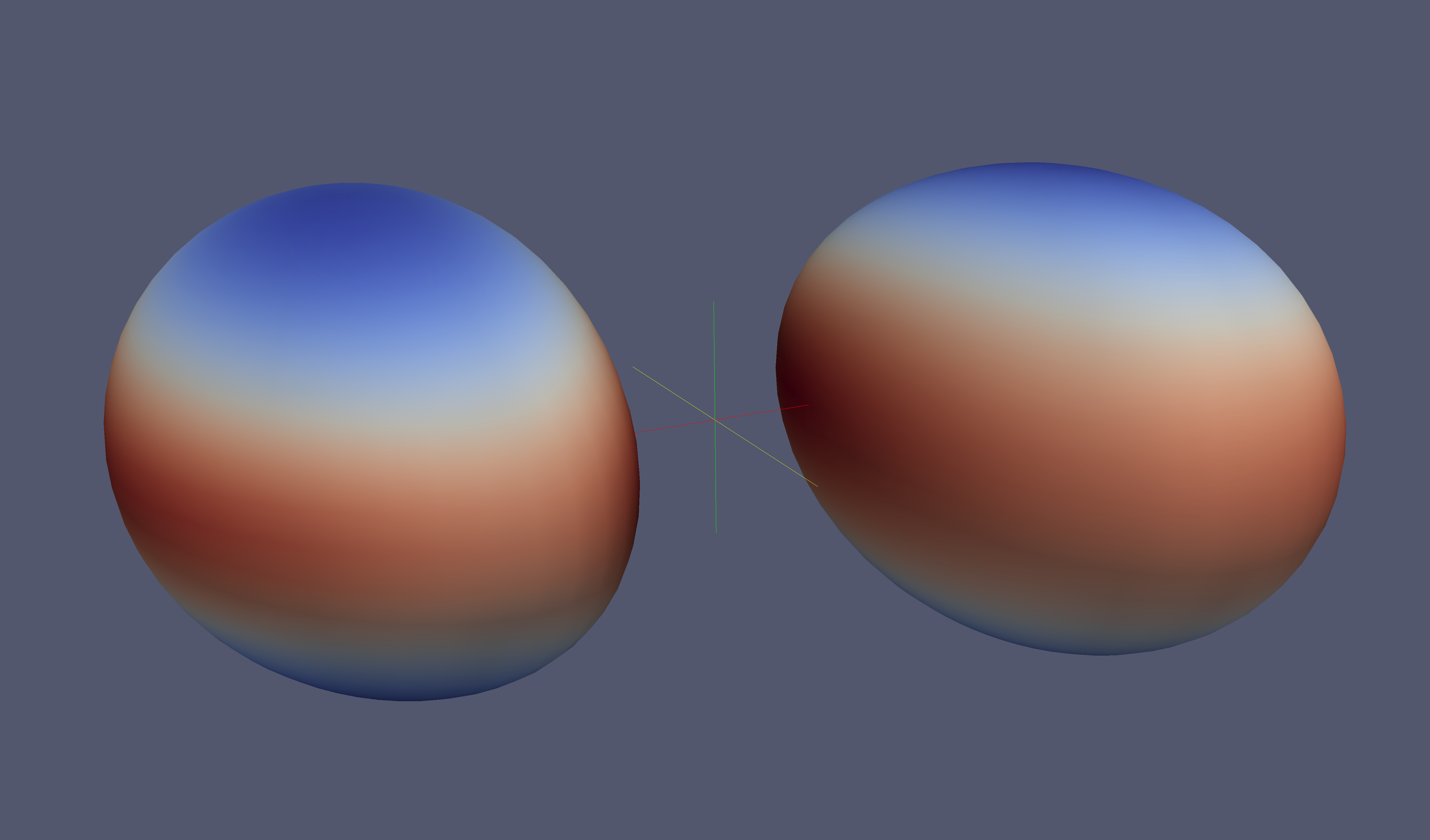
Using the fast-flow method described in Ref. Gundlach (1998), we find the apparent horizons as an expansion in spherical harmonics, truncated at a given maximum order $\ell$. As the system evolves, we adaptively change $\ell$ to satisfy accuracy criteria for the resolution of the horizon. After a common horizon is found during merger, the evolution continues on a new domain with a single excision surface that subsumes the two individual excision regions Szilágyi et al. (2009).

We measure the quasi-local spin, $S$, on each horizon using the approximate Killing vector method described in Ref. Lovelace et al. (2008). The dimensionless spin is then

$$\chi=\frac{S}{M_{\rm Ch}^{2}},$$ (1)

where $M_{\rm Ch}$ is the Christodoulou mass,

$$M_{\rm Ch}^{2}=M_{\rm irr}^{2}+\frac{S^{2}}{4M_{\rm irr}^{2}},$$ (2)

and $M_{\rm irr}$ is the irreducible mass, which is a function of the horizon area,

$$M_{\rm irr}=\sqrt{\frac{A_{\rm AH}}{16\pi}}.$$ (3)

With these definitions, $\chi=1$ represents an extremal black hole Booth and Fairhurst (2008).

We choose an integer $k$ to characterize the resolution of each simulation. We call $k$ the resolution level (or “Lev”). It sets the resolution by defining the target maximum truncation error for the adaptive mesh refinement and adaptive horizon finding as

$$\epsilon_{\rm max}=10^{-4}e^{-k}.$$ (4)

Around the excision boundary, where the most resolution is required, we reduce the target maximum truncation error for adaptive mesh refinement by a factor of $10^{2}$.

III Simulations

There are ten new simulations presented in this paper: $S^{++}_{0.95}$, $S^{++}_{0.9}$, $S^{++}_{0.85}$, $S^{++}_{0.8}$, $S^{++}_{0.6}$, $S^{++}_{0.2}$, $S^{--}_{0.2}$, $S^{--}_{0.6}$, $S^{--}_{0.8}$, and $S^{--}_{0.9}$. Initial data were generated with a target Christodoulou mass for each hole $M_{0}=0.5$, target spin for each hole $\chi_{0}$, and target ADM linear momentum $p_{0}^{i}=0$. We fix the initial separation at $d_{0}=15.366M$, and then we iterate as summarized in Sec. II to obtain the initial radial velocity $\dot{d}_{0}/d_{0}$ and angular velocity $\Omega_{0}$. The targets are met to within an absolute error of $\mathcal{O}(10^{-8})$, and the resulting initial data parameters are reported in Table 1. We construct our initial data with a target total Christodoulou mass of $M=1$ so that our evolution code units are essentially interchangeable with units of $M$.

$\chi_{0}$	$M\dot{d}_{0}/d_{0}\times 10^{4}$	$M\Omega_{0}$	$N_{\rm orbits}$
0.95	7.26420673	0.01395360	25.4
0.9	5.48222492	0.01419573	24.9
0.85	4.33347923	0.01437107	24.7
0.8	3.54332917	0.01450430	24.2
0.6	1.65215665	0.01487274	22.8
0.2	0.09507527	0.01525060	19.9
-0.2	-0.69081937	0.01538827	17.2
-0.6	-1.95883097	0.01527384	14.6
-0.8	-3.60252091	0.01501397	13.3
-0.9	-5.42657163	0.01474328	12.8

Table 1: Initial data parameters (radial velocity $\dot{d_{0}}$ and angular velocity $\Omega_{0}$) at separation $d_{0}=15.366M$ for the ten new simulations with target spin, $\chi_{0}$. Also included is the approximate number of orbits until merger. Here $M$ is the sum of the Christodoulou masses at time $t=0$.

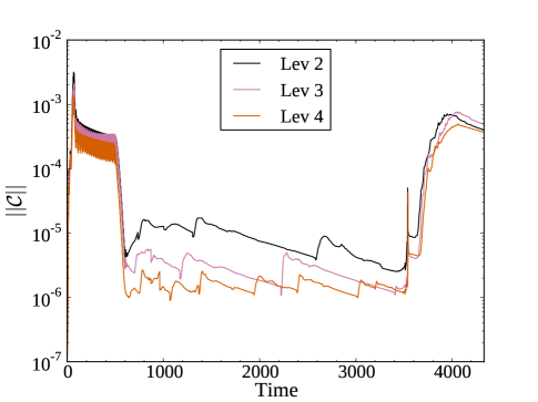
At least three different resolutions were evolved for each case to check convergence. Figure 2 shows convergence of the (normalized) volume-averaged $L^{2}$-norm of the generalized harmonic constraint energy Lindblom et al. (2006) for a representative case. Each time the domain structure is changed to alleviate grid compression, the constraints jump because of interpolation errors, but then slowly decay back to their baseline levels.

Figure 2: Normalized constraint violations for $S^{--}_{0.9}$. For each resolution level, $k$, we plot $||\mathcal{C}||$, the volume-averaged $L^{2}$-norm of the generalized harmonic constraint energy divided by the volume-averaged $L^{2}$-norm of the dynamical field gradients. This measure is defined in Eq. (71) of Ref. Lindblom et al. (2006). As the resolution level increases, the constraints decrease. Jumps in the constraints are attributed to changes in the domain structure, and the spike around $t\sim 3500M$ corresponds to the merger.

Additional simulations are used in our analysis of masses and spins in Sec. IV: $S^{++}_{0.97}$ Lovelace et al. (2012), $S^{++}_{0.44}$ Chu (2012), $S^{--}_{0.0}$ Garcia et al. (2012), $S^{--}_{0.44}$ Chu et al. (2009), and $S^{--}_{0.95}$ Lovelace et al. (2011). Although these have been previously reported, we include them below for completeness. It should be noted that $S^{++}_{0.44}$ and $S^{--}_{0.44}$ are older simulations and therefore used different initial data and evolution machinery than described in Sec. II. Simulations $S^{--}_{0.95}$, $S^{--}_{0.0}$, and $S^{++}_{0.97}$ used the initial data methods of Sec. II, but earlier implementations of the evolution methods.

III.1 Mass and spin

Figure 3: Plots of the apparent horizon quantities as a function of time for a representative case, $S^{++}_{0.9}$. The top panels display the dimensionless spin and the bottom panels display the Christodoulou mass. From left to right, the panels display the inspiral, merger, and ringdown. We normalize the $y$-scales separately so that the differences between each resolution can be clearly seen. The discontinuity in the middle panel indicates where we begin to measure the mass and spin on the common horizon. The dots in the early inspiral identify our choice of $t_{i}$ for each resolution level.

We define the initial spin, $\chi_{i}$, to be the spin after the system has relaxed from the initial data and the junk radiation at the apparent horizon has become negligible. The spin before this time is not physically relevant to the rest of the evolution. There are subtle issues to consider when choosing the time to measure $\chi_{i}$. If we choose too early a time, then junk radiation effects will still be present. If we are overly cautious and choose too late a time, then the system will have emitted enough gravitational radiation to significantly change the spin.

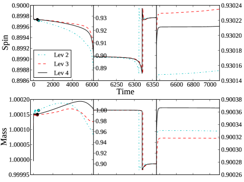
We use a histogram method to determine $\chi_{i}$. Let $\{\chi_{I}\}$ be the set of spin measurements during the inspiral. The range of $\{\chi_{I}\}$ is split uniformly into $N$ bins, where $N$ is the size of $\{\chi_{I}\}$, and then each element of $\{\chi_{I}\}$ is put into the appropriate bin. We choose $\chi_{i}=\chi(t_{i})$, where $t_{i}$ is the latest time when the spin is in the bin containing the most measurements. In the initial relaxation, the spin is oscillating, and during the inspiral, the spin changes more rapidly as the holes approach each other. Under these conditions, this method selects the spin just after the junk radiation, when the spin is nearly constant for a long interval. Figure 3 shows the evolution of the mass and spin as a function of time for a representative case, and identifies our choice of $t_{i}$ by the dots in the early inspiral.

Case	$|\chi_{i}|$	$|\chi_{f}|$
$S^{--}_{0.95}$	0.949053(-30)	0.37567(-18)
$S^{--}_{0.9}$	0.899569(-11)	0.392748(-12)
$S^{--}_{0.8}$	0.7997602(59)	0.4268932(30)
$S^{--}_{0.6}$	0.59993163(71)	0.4942327(-31)
$S^{--}_{0.44}$	0.437568970(-10)	0.547851(20)
$S^{--}_{0.2}$	0.1999802(-40)	0.6242202(-61)
$S^{--}_{0.0}$	64(-29)$\times 10^{-8}$	0.686445(-52)
$S^{++}_{0.2}$	0.200035(-19)	0.7464314(-96)
$S^{++}_{0.44}$	0.4365505(95)	0.8140(10)
$S^{++}_{0.6}$	0.5999635(14)	0.857808(15)
$S^{++}_{0.8}$	0.7998737(-44)	0.907526(14)
$S^{++}_{0.85}$	0.849826(15)	0.919088(30)
$S^{++}_{0.9}$	0.8997371(-15)	0.930212(23)
$S^{++}_{0.95}$	0.9495863(-25)	0.940852(29)
$S^{++}_{0.97}$	0.969504(13)	0.944964(11)

Table 2: Dimensionless spin measurements. For each case, we provide the initial spin magnitude of each hole and the final spin magnitude of the remnant at the highest resolution. Note that the number in parentheses is not an error estimate, but provides the value at the next highest resolution when added to the last two significant digits.

We compute $t_{i}$ from $\chi$ because the behavior of the mass is not as simple during the inspiral. The histogram method applied to the mass will pick out the local maximum late in the inspiral that is present in most of our cases (see Fig. 3). We define the initial mass to be $M_{i}=M(t_{i})$, the sum of the Christodoulou masses at time $t_{i}$.

The final spin and Christodoulou mass, $\chi_{f}$ and $M_{f}$, are measured at the last observation time, when the merger remnant is in quasi-equilibrium and approximates a Kerr black hole. We report the initial and final spins in Table 2, and the initial and final Christodoulou masses in Table 3.

Case	$M_{i}$	$M_{f}$	$E_{\rm rad}(\%)$
$S^{--}_{0.95}$	0.999856(68)	0.968134(33)	3.1727(33)
$S^{--}_{0.9}$	1.00016197(73)	0.967909(-27)	3.2248(28)
$S^{--}_{0.8}$	1.0000859(-11)	0.9665941(-16)	3.348894(50)
$S^{--}_{0.6}$	1.00002292(-78)	0.963769(-14)	3.6253(13)
$S^{--}_{0.44}$	2.2470608(-22)	2.159561(-49)	3.8940(21)
$S^{--}_{0.2}$	0.999956(26)	0.9564388(84)	4.3519(17)
$S^{--}_{0.0}$	0.9999971(-43)	0.9516182(-74)	4.83791(33)
$S^{++}_{0.2}$	0.999961(22)	0.945471(16)	5.44923(46)
$S^{++}_{0.44}$	2.2451548(28)	2.10099(-44)	6.421(20)
$S^{++}_{0.6}$	1.00001907(-96)	0.926868(-19)	7.3149(18)
$S^{++}_{0.8}$	1.0000765(-22)	0.911275(-28)	8.8794(26)
$S^{++}_{0.85}$	1.000108(-12)	0.906168(-73)	9.3931(62)
$S^{++}_{0.9}$	1.0001513(-29)	0.900366(-48)	9.9770(46)
$S^{++}_{0.95}$	1.00021743(77)	0.893703(-65)	10.6492(66)
$S^{++}_{0.97}$	1.0002384(-94)	0.890691(-22)	10.9521(14)

Table 3: Christodoulou mass measurements. For each case, we provide the total initial mass of the black holes, the final mass of the remnant, and the radiated energy computed from Eq. (5) at the highest resolution. Note that the number in parentheses is not an error estimate, but provides the value at the next highest resolution when added to the last two significant digits.

From the initial and final Christodoulou masses, we can infer the fraction of the black hole energy that is radiated in gravitational waves during the evolution:

$$E_{\rm rad}=1-\frac{M_{f}}{M_{i}}.$$ (5)

We expect mass and spin measurements at higher resolutions to be more accurate. However, as illustrated by the comparisons in Fig. 4, these quantities are not strictly convergent in a number of cases. For this reason, we include measurements from all resolutions in our analysis in Sec. IV and weight the uncertainty in the error assigned to a particular measurement by a function of resolution level $k$.

As described in Sec. II, the most stringent resolution requirements occur in the vicinity of the apparent horizons, but the accuracy may be dominated by short, under-resolved segments of the evolution. The initial masses and spins appear to be randomly perturbed by the junk radiation as the initial data relax. The final masses and spins, which are already limited by the accuracy of the initial masses and spins, appear to also be affected by the details of the coalescence, where we see a spike in constraint violations (Fig. 2). Apart from these under-resolved segments, we do see convergence in the time derivatives of the masses and spins, but the absolute values remain offset from one another.

Figure 4: Differences in the final masses and spins between resolution levels. For each case, we compare $\chi_{f}$ and $M_{f}$ of the highest resolution to the two lower resolutions. Note that, except for the older $S^{\pm\pm}_{0.44}$ simulations, all differences are $\lesssim 10^{-4}$. Differences in the initial masses and spins behave similarly.

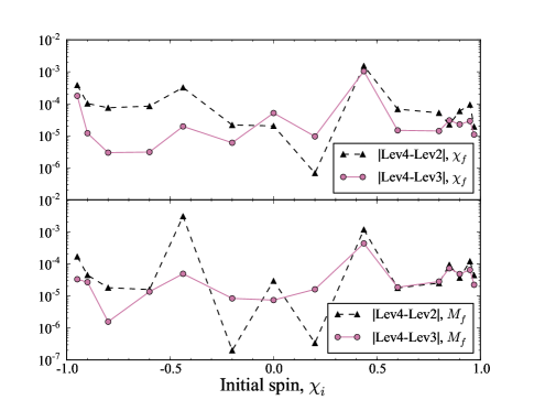
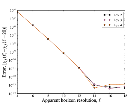
We have investigated other potential sources of uncertainty, but found them to lie below the resolution level uncertainty. For example, one source of uncertainty in the masses and spins is the resolution of the surface of the horizon. In Fig. 5, we show a representative plot of error in final spin as a function of $\ell$ of the horizon finder. Let $\Delta\chi_{k}$ be the resolution level error between the two highest resolutions, and let $\Delta\chi_{\ell}$ be the resolution error between the $\ell$ chosen by the adaptive horizon finder and the $\ell$ for which the horizon is fully resolved. At the final time of the simulation, we find that, in all cases, $\Delta\chi_{k}>\Delta\chi_{\ell}$ by several orders of magnitude.

Figure 5: Convergence of the final spin for $S^{--}_{0.9}$ as a function of the $\ell$ of the horizon finder. We plot the difference between $\chi_{f}(\ell)$ and $\chi_{f}(\ell=20)$ for each resolution. The adaptive horizon finder for this case chose $\ell=8$ at the final time of the simulation.

A source of uncertainty in the radiated energy is the energy that would have been radiated by the binary as it proceeds from infinite separation to the separation $d_{0}$ at which we start the simulation. As discussed in Ref. Lovelace et al. (2012), Alvi’s formula Alvi (2001) estimates that the energy radiated from $d=\infty$ to $d=d_{0}$ is one part in $10^{6}$. Since this is smaller than our resolution level uncertainty, it is safe to ignore this difference and we can think of $E_{\rm rad}$ as the total radiated energy from infinite separation through ringdown.

IV Results

Much effort has been put into constructing phenomenological formulae for the final spin Campanelli et al. (2006); Rezzolla et al. (2008); Barausse and Rezzolla (2009); Tichy and Marronetti (2008) and radiated energy Campanelli et al. (2006); Tichy and Marronetti (2008); Reisswig et al. (2009); Barausse et al. (2012) as a function of initial spin. Because the SpEC code has the capability to generate and evolve initial data of black holes with spins above the “Bowen-York limit” of $\chi\approx 0.93$ Hannam et al. (2009), we are able to provide new data points to test and improve these formulae.

We use a Bayesian nonlinear measurement error model (described in Appendix A) to fit and compare new parametric formulae. This approach (1) accounts for uncertainties in both the initial spin data and the output data (i.e., final spin or radiated energy); (2) accounts for the expected improvement in accuracy of results as the resolution level increases; and (3) includes a simple systematic error component quantifying misfit between a chosen formula and the curve the data are converging toward. The framework lets us predict an output as a function of initial spin, with prediction uncertainties that account for the uncertainties in the parameters of the chosen formula (including correlated uncertainties) and the typical scale of the systematic error.

The new fitting formulae that we provide here are only applicable to equal mass binary black hole configurations with equal spins aligned or anti-aligned with the orbital angular momentum. More general formulae exist (see e.g. Refs. Lousto et al. (2010); Gergely and Biermann (2012); Barausse and Rezzolla (2009); Tichy and Marronetti (2008)), but they are less accurate at high spins because of the scarcity of simulations with both unequal masses and high spins in random orientations.

IV.1 Final spin

Using the data from Table 2, we construct a new fitting formula for the final spin as a function of initial spin. We fit to a fourth-order polynomial,

$$\tilde{\chi}_{f}=a_{0}+a_{1}\chi_{i}+a_{2}\chi_{i}^{2}+a_{3}\chi_{i}^{3}+a_{4}\chi_{i}^{4}.$$ (6)

The best fit to our data has the parameters $a_{n}$ and associated covariance $\Sigma_{a}$:

$$a =\left(\begin{array}[]{r}a_{0}\\ a_{1}\\ a_{2}\\ a_{3}\\ a_{4}\end{array}\right)=\left(\begin{array}[]{r}0.686402(60)\\ 0.30660(14)\\ -0.02684(33)\\ -0.00980(19)\\ -0.00499(35)\end{array}\right)$$ (17)

$$\Sigma_{a} =\left(\begin{array}[]{rrrrr}3.6&0.31&-14&-0.45&11\\ 0.31&21&-4.8&-26&6.0\\ -14&-4.8&110&7.1&-110\\ -0.45&-26&7.1&36&-9.5\\ 11&6.0&-110&-9.5&120\end{array}\right)\times 10^{-9}$$ (23)

The uncertainty in $a_{n}$, given in parentheses in Eq. (17), is estimated by $\sqrt{\Sigma^{nn}_{a}}$. However, the parameter estimates are highly correlated; therefore, the full covariance matrix is used in the computation of the fit uncertainty $\sigma_{f}$ in Eq. (49). In Fig. 6, we show the fit and residuals using Eq. (6) with the parameters from Eq. (17).

Figure 6: In the top panel, we plot our preferred fitting formula (solid line), the fourth-order polynomial in Eq. (6), and a comparison with a second-order polynomial (dashed line) for $\chi_{f}$ as a function of $\chi_{i}$. Our data points are plotted as polygons, where more sides indicates higher resolution level. In the bottom panel, we plot the residuals of the fourth-order polynomial. We indicate our fit parameter (dotted line) and total prediction (dashed line) uncertainties (defined in Appendix A), which in this case are nearly identical. Note that the residuals for the two lower resolution runs for $S^{++}_{0.44}$ are too large to fit in this panel.

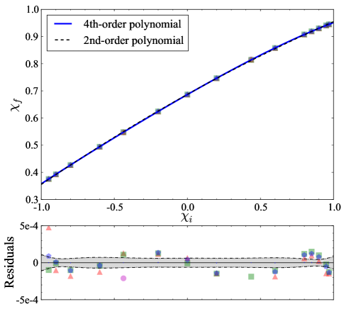
We fit to a fourth-order polynomial because the high accuracy of our dataset enables us to identify significant third- and fourth-order trends in the residuals of a fit to a second-order polynomial, which is the fitting function used in Refs. Rezzolla et al. (2008); Barausse and Rezzolla (2009); Tichy and Marronetti (2008). The difference between the logarithm of the marginalized likelihood function (LML) for the best-fit fourth-order and second-order polynomials is $\mathchar 21016\relax 40$, indicating that the fourth-order polynomial provides a significantly better fit. If the two additional degrees of freedom were fitting noise, rather than some underlying structure in the data, then we would only expect a change in maximum LML of $\mathcal{O}(1)$.

The estimated systematic error magnitude $\hat{\sigma}_{\Delta}$ (defined in Appendix A) for the fourth-order polynomial formula is negligibly small, suggesting that the significant behavior is captured as well as could be expected. However, the residuals, especially at large aligned spins, display trends suggesting that there is additional structure not captured by the fourth-order polynomial (such trends are ignored by our simple systematic error model). This encouraged us to explore a fifth-order polynomial formula, but it did not reduce the residuals enough to justify the additional degree of freedom. This does not rule out the possibility that a different formula could capture the behavior even more accurately.

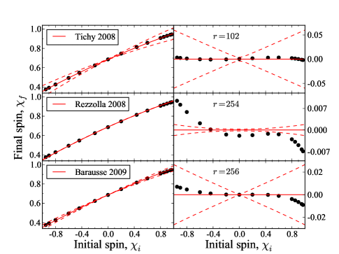
We compare our data to existing fitting formulae for the final spin in Fig. 7. The $\chi_{f}$ data corroborate the existing fitting formulae, but indicate deviations at large spins (especially in the aligned direction). This is an expected consequence of the scarcity of high spin numerical relativity data heretofore. In the figure, we provide a quantity for each fit, $r$, that measures how much larger its systematic error is than that of our fourth-order polynomial. This is essentially a ratio of the root-mean-square residuals (more precisely, $r$ is the ratio of the $\hat{\sigma}_{\Delta}$ values). The previously reported formulae have roughly 100 to 250 times as much systematic error as our fourth-order polynomial fit. While the formula in Tichy 2008 Tichy and Marronetti (2008) performs best, we note that it has a large uncertainty.

Figure 7: Final spin as a function of initial spin. In the left panels we plot our data (circles) along with the fitting formula (red line) with error estimates (dashed) from several other studies. The top panel is from Ref. Tichy and Marronetti (2008), the middle is from Ref. Rezzolla et al. (2008), and the bottom is from Ref. Barausse and Rezzolla (2009). In the right panels we plot the difference between our data and the corresponding fitting formula on the left. The value $r$ quantifies the size of the systematic error compared to the fourth-order polynomial.

IV.2 Radiated energy

Following the procedure in Sec IV.1, we use the data from Table 3 to construct a new fitting formula for the radiated energy fraction, $E_{\rm rad}$, as a function of initial spin. We fit to a hyperbolic function,

$$\tilde{E}_{\rm rad}=b_{0}+\frac{b_{1}}{b_{2}+\chi_{i}}.$$ (24)

The best fit to our data has the parameters $b_{n}$ and associated covariance $\Sigma_{b}$:

$$b =\left(\begin{array}[]{r}b_{0}\\ b_{1}\\ b_{2}\end{array}\right)=\left(\begin{array}[]{r}0.00258(29)\\ -0.07730(79)\\ -1.6939(59)\end{array}\right)$$ (31)

$$\Sigma_{b} =\left(\begin{array}[]{rrr}0.83&2.2&16\\ 2.2&6.2&46\\ 16&46&350\end{array}\right)\times 10^{-7}$$ (35)

The uncertainty in $b_{n}$, given in parentheses in Eq. (31), is estimated by $\sqrt{\Sigma^{nn}_{b}}$. In Fig. 8, we show the fit and residuals using Eq. (24) with the parameters from Eq. (31).

Figure 8: In the top panel, we plot our preferred fitting formula (solid line), the hyperbolic function in Eq. (24), and a comparison with a second-order polynomial (dashed line) for $E_{\rm rad}$ as a function of $\chi_{i}$. Our data points are plotted as polygons, where more sides indicates higher resolution level. In the bottom panel, we plot the residuals of the hyperbolic function. We indicate our fit parameter (dotted line) and total prediction (dashed line) uncertainties (defined in Appendix A).

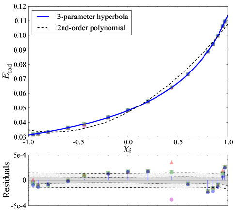
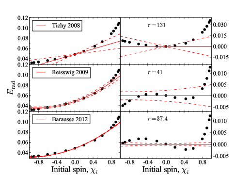
We use a hyperbolic fitting function instead of a second-order polynomial (as in Refs. Tichy and Marronetti (2008); Reisswig et al. (2009)) or a constrained second-order polynomial, e.g. $\tilde{E}_{\rm rad}=c_{0}+c_{1}\chi_{i}+(c_{1}/4)\chi_{i}^{2}$ (as in Ref. Barausse et al. (2012)). Parabolic fits show visible offsets in various regions of the initial spin space, which can be seen in plots of the residuals in Barausse et al. (2012) and in the comparison plot in the top panel of Fig. 8. The difference between the maximum LML for the 3-parameter hyperbola and the second-order polynomial is $\mathchar 21016\relax 36$, indicating that the hyperbola is a dramatically better fit to the data.

In Fig. 9, we compare our data to existing fitting formulae for $E_{\rm rad}$. All previous formulae suffer from the same systematic deficiencies as the best second-order polynomial fit to our data shown in Fig. 8. The ratio of the systematic error magnitude in these formulae to its magnitude in our 3-parameter hyperbolic fit, $r$, is shown in the figure and ranges from roughly 40 to 130. Note that it is not meaningful to compare these $r$ values to those shown in Fig. 7, because we have not added any additional degrees of freedom in our $E_{\rm rad}$ model compared to a second-order polynomial (unlike in our final spin model, which adds two degrees of freedom).

Figure 9: $E_{\rm rad}$ as a function of initial spin. In the left panels we plot our data (circles) along with the fitting formula (red line) with error estimates (dashed) from several other studies. The top panel is from Ref. Tichy and Marronetti (2008), the middle is from Ref. Reisswig et al. (2009), and the bottom is from Ref. Barausse et al. (2012). In the right panels we plot the difference between our data and the corresponding fitting formula on the left. The value $r$ quantifies the size of the systematic error compared to the 3-parameter hyperbola.

IV.3 Extremality

An important aspect of these fitting formulae is their ability to predict remnant properties for nearly extremal initial spins. How much of the initial mass can be radiated as gravitational waves, and how fast can the remnant hole spin? Our prediction for the radiated energy and final spin for an extremal initial spin configuration, $\chi_{i}=1$, is

$$\tilde{E}_{\rm rad}(1) =0.11397(18),$$ (36)

$$\tilde{\chi}_{f}(1) =0.951383(85),$$ (37)

where the uncertainty (in parentheses) is $\sigma_{\rm tot}$, the total prediction uncertainty defined in Eq. (50), evaluated at $\chi_{i}=1$. The highest radiated energy predicted by any of the formulae we compare against in this paper is $E_{\rm rad}(1)=0.0995(8)$.

Previous estimates of $E_{\rm rad}$ underestimated the mass loss for large, aligned initial spins. The most extreme data point in this paper, $S^{++}_{0.97}$, was identified as a potential outlier Barausse et al. (2012) and $E_{\rm rad}$ was expected to be $\lesssim 10\%$ for an extremal, aligned configuration inspiraling from infinity. Additional data presented here, most notably $S^{++}_{0.95}$ and $S^{++}_{0.9}$, suggest that $S^{++}_{0.97}$ is not an outlier. Furthermore, these cases indicate that even a $\chi_{i}=0.9$ inspiral is capable of radiating $\gtrsim 10\%$ of its initial mass.

Simulations with $\chi_{i}>0.93$ are an important factor in our fitting formulae. This high-spin regime is not accessible with the most popular initial data methods for binary black hole evolutions, which assume conformal flatness (cf. Ref. Lovelace et al. (2008) and references therein). To assess the impact of the high spin simulations, we compare our best fits to fits of a subset of the data, omitting cases $S^{--}_{0.95}$, $S^{++}_{0.95}$, and $S^{++}_{0.97}$. We identify several key results.

For the $\chi_{f}$ formula, we find that $\Delta\tilde{\chi}_{f}(1)\gtrsim 2.5\sigma_{\rm tot}^{\rm sub}(\chi_{f},1)$. That is, the prediction of the final spin with the full dataset differs from the prediction with the subset by more than 2.5 times the total prediction uncertainty in the fit to the subset. The parameter uncertainty in the full dataset is smaller by a factor $\sigma_{f}/\sigma_{f}^{\rm sub}\approx 0.6$, which is much smaller than would be expected from adding 3 data points randomly distributed in initial spin (the expected improvement based on the root-$N$ rate would be $\sqrt{12/15}\approx 0.9$). In a random sampling context, one would typically have to more than double the size of the dataset to get such a reduction in parameter uncertainties. Of course, we have not chosen the subset randomly. Note that because the systematic error magnitude is negligible, $\hat{\sigma}_{\Delta}\approx 0$, the total prediction uncertainty of Eq. (50) has the same behavior as the parameter uncertainty.

For the $E_{\rm rad}$ formula, we find that $\Delta\tilde{E}_{\rm rad}(1)\gtrsim 3.5\sigma_{\rm tot}^{\rm sub}(E_{\rm rad},1)$; the lower spin subset poorly predicts the extremal $E_{\rm rad}$. Parameter uncertainties decrease only slightly faster than the expected root-$N$ rate for adding 3 randomly placed data points, $\sigma_{f}/\sigma_{f}^{\rm sub}\approx 0.85$. However, the total prediction uncertainty at $\chi_{i}=1$ increases, $\sigma_{\rm tot}/\sigma_{\rm tot}^{\rm sub}\approx 1.15$, because the additional high spin data deviate most from the fitting formula that is based on lower spin data. That is, $E_{\rm rad}$ for $\chi_{i}>0.93$ is unanticipated by the fit to the lower spin subset, causing the systematic error magnitude $\hat{\sigma}_{\Delta}$ to increase. While this highlights the importance of the high spin data in assessing the predictive power of the fitting formula for near-extremal initial spins, it also suggests that we are unlikely to capture the behavior of $E_{\rm rad}$ much better with our simple fitting formula. Furthermore, neither manual nor algorithmic searches Schmidt and Lipson (2009) have identified any better formulae, which leads us to believe that for the best predictive results at high spins, a non-parametric approach may be preferred. Such an approach could be implemented using, for example, a correlated Gaussian process Rasmussen and Williams (2006), which would provide a way to predict final masses and spins without the use of a parametric fitting formula.

The analysis comparing the subset to the full dataset does not change in any appreciable way if we use a near-extremal spin, e.g. $\chi_{i}=0.97$, instead of the most extreme case, $\chi_{i}=1$.

V Conclusions

In this paper, we present and analyze a family of numerical relativity simulations performed using SpEC in order to construct improved fitting formulae for the final spin and radiated energy as a function of initial spin. We consider a physically motivated, one-dimensional subset of the binary black hole parameter space, in which the black holes have equal masses and equal spins aligned or anti-aligned with the orbital angular momentum. The improvement in these fitting formulae is most dramatic in the regime where the initial spin is above the “Bowen-York limit,” since for the first time data from simulations above this limit have been included in the fits.

For the final spin, we improve on the second-order polynomial fitting formula by using a fourth-order polynomial to capture the statistically significant cubic and quartic features. For the radiated energy, we find that a 3-parameter hyperbolic fitting formula is greatly preferred to a second-order polynomial. The qualitatively different behavior at large, aligned spins in the new fit to $E_{\rm rad}$ implies that there is somewhat more power in gravitational waves from nearly extremal sources than previously thought, perhaps because of higher-order effects that become relevant at very high spins.

We have shown that performing more nearly extremal simulations is the most effective way to reduce the uncertainty in the fitting formula parameters. However, we have also observed that the systematic uncertainty in $E_{\rm rad}$ may prohibit a simple fitting formula from providing any further significant improvement to the prediction uncertainty of $E_{\rm rad}$ for high, aligned spins.

Analytic models, such as the aligned-spin EOB model, are needed to generate templates for gravitational-wave detectors (e.g. LIGO), because of the prohibitive expense of generating sufficient numerical relativity data to adequately cover the parameter space. The fitting formulae we define in this paper can be used to better calibrate these models, and therefore improve future template waveforms.

Appendix A Method for constructing our fitting formulae

Our goal is to find a convenient but reasonably accurate function that predicts the final black hole spin, $\chi_{f}$, or the fractional radiated energy, $E_{\rm rad}$, as a function of the initial spin, $\chi_{i}$. We will specify one or more simple parametric candidate functions, find the best parameter values, quantify uncertainties in the parameters and predictions, and compare rival candidate functions. To treat both the $\chi_{f}$ and $E_{\rm rad}$ problems in generic notation, we let $\xi$ denote the predictor (i.e., $\chi_{i}$), and $\eta$ denote the response we seek to predict (i.e., $\chi_{f}$ or $E_{\rm rad}$). We have one or more parametric models for the relationship, $\eta\approx f(\xi;\theta)$, with parameters $\theta$ (we sometimes suppress the parameter dependence below to simplify notation).

The data for the analysis are from post-processing outputs from deterministic numerical calculations of the binary black hole merger. A complex computation produces initial data (ID) targeting a specified value of $\xi$, but the actual value of $\xi$ that the generated ID corresponds to necessarily differs from the target value. A processing algorithm estimates the actual value to be $x$. Evolution of the ID produces high-dimensional outputs that are processed to produce the computed response, $y$, that estimates the result, $\eta$, that would be obtained by solving the PDEs exactly. A set of $(x,y)$ pairs constitutes the basic data we must use to find $f(\xi;\theta)$.

A variety of parameters govern the accuracy of the ID, evolution, and processing algorithms. These are summarized via a resolution level $k$ (defined in Sec. II) assigned to each $(x,y)$ pair, with the $x$ and $y$ values likely to be closer to the $\xi$ and $\eta$ values when $k$ is larger. For every choice of ID, we have results for multiple values of $k$, comprising repeated measurements of $(\xi,\eta)$ of varying accuracy.

We have developed a Bayesian nonlinear measurement error model for the analysis. Letting the index $n$ label the choice of ID, the model specification is:

$$x_{nk} =\xi_{n}+\epsilon_{nk},$$ (38)

$$y_{nk} =\eta_{n}+\delta_{nk}$$ (39)

$$=f(\xi_{n};\theta)+\Delta_{n}+\delta_{nk},$$ (40)

for $N$ ID cases ($n=1$ to $N$), and $k\in L_{n}$ for ID case $n$, where $L_{n}$ denotes a set of levels run for case $n$ (for most cases, $L_{n}=\{2,3,4\}$, but for runs targeting $\chi_{i}=\pm 0.44$, $L_{n}=\{1,2,3\}$). Here $\epsilon_{nk}$ and $\delta_{nk}$ denote level error terms reflecting the difference between numerical results at finite resolution and the actual solution to the differential equations we are studying. For Eq. (40) we set $\eta_{n}=f(\xi_{n};\theta)+\Delta_{n}$, where $\Delta_{n}$ is a discrepancy term representing the difference between the true response and the prediction based on the fitting function.

To complete the model we must assign (prior) probability density functions (PDFs), i.e. priors, to a number of random variables: the level errors, $\epsilon_{nk}$ and $\delta_{nk}$; the latent predictor variables, $\xi_{n}$; and the latent discrepancy variables, $\Delta_{n}$.

We assign independent, zero-mean normal distributions to the level error terms, $\epsilon_{nk}$ and $\delta_{nk}$, with standard deviations $\sigma_{x}/\alpha_{k}$ and $\sigma_{y}/\alpha_{k}$ (respectively). We assign $\alpha_{k}$ scale factors to capture the notion that we expect the errors to be smaller (on average) for higher levels. For the calculations here, we took $\alpha_{k}=(1/2)^{4-k}$, so the standard deviations for the highest-resolution $k=4$ results are $\sigma_{x}$ and $\sigma_{y}$, and the error scales double for each decreasing level. We did not explore this assignment except to verify that this choice has a much higher likelihood than taking $\alpha_{k}=1$, i.e., the data themselves show clear evidence for convergence as $k$ grows. Although in principle we could let the error scale be different for each ID case, for simplicity we assign a common error scale across ID cases; the modest amount of data we have does not indicate a strong variation of error scale with ID. We adopt normal distributions, partly for convenience, but also because we are modeling relationships between scalar quantities calculated from high-dimensional computational outputs with complicated algorithms. Presuming the final errors result from numerous additive contributions whose uncertainties have finite variance, the central limit theorem motivates the normal choice.

We assign informative but relatively broad priors for the $\xi_{n}$ values, reflecting the ability to produce ID corresponding to a $\xi_{n}$ value close to a desired target value, $\mu_{n}$. The priors are normal with means $\mu_{n}$ (equal to the target value for ID case $n$) and common standard deviation $w=0.002$, reflecting the typical change in mass and spin as a result of the initial relaxation (as seen in Fig. 3). These values do not strongly impact the results.

We also assign independent, zero-mean normal distribution PDFs to the discrepancy terms, with common standard deviation $\sigma_{\Delta}$. The quantity $\sigma_{\Delta}$ represents the typical scale of systematic error magnitude in the model. A more flexible and realistic choice would be to assign a correlated Gaussian process prior over the space of discrepancy functions, $\Delta(\xi_{n})$, and to identify $\Delta_{n}=\Delta(\xi_{n})$. This would resemble the practice in the literature on Bayesian emulation of input/output response surfaces, the prevailing approach in the literature on the statistical analysis of the results of deterministic numerical simulations (see, e.g., Kennedy and O’Hagan (2001); Higdon et al. (2004)). But the goal of that literature is not to find simple and tractable fitting functions; it instead builds nonparametric emulators that, while simpler than the simulators being emulated, are still computationally nontrivial. Moreover, the vast majority of existing work on emulation addresses cases with precisely known inputs, which is not the case here; uncertainty in the predictor significantly complicates implementation of Gaussian process regression McHutchon and Rasmussen (2011); Dallaire et al. (2011). The independent normal PDF for $\Delta_{n}$ will enable us to invoke a simple approximation leading to analytical results.

Finally, we adopt flat priors for the fitting function model parameters, $\theta$.

The conditional dependency structure of such a multilevel model can be represented by a directed acyclic graph (DAG). A graphical model of this type can be readily coded in a DAG-oriented statistical modeling language (e.g., WinBUGS or JAGS) to enable Bayesian computation via Markov chain Monte Carlo (MCMC) posterior sampling. Here the focused goal (finding a simple fitting function) and the small uncertainties in the level error terms (well below 1% for nonzero spins) motivated an analytical approach based on linearization of $f(\xi)$. This lets us avoid the complexity of MCMC, producing a fast algorithm that is relatively simple to use.

Figure 10 shows the DAG for our model. Circles denote random variables (RVs, uncertain quantities with assigned or computed PDFs). Shaded circles are the data $(x,y)$, and shaded squares are fixed constants that help define the model. We marginalize over the error RVs ($\epsilon_{nk}$, $\delta_{nk}$, and $\Delta_{n}$) and the uncertain input variables ($\xi_{n}$), and then we solve for the remaining non-shaded variables simultaneously. The plates (enclosing boxes) denote parts of the graph that are replicated as indicated by the quantity in the lower right corner of each plate.

Figure 10: Directed acyclic graph displaying the conditional dependence structure of the Bayesian nonlinear measurement error model adopted for the fitting function analysis. See text for a detailed description.

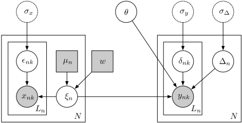
Dashed circles indicate RVs that play the role of hyperparameters, i.e., parameters defining prior PDFs for lower-level RVs. Formally, we could account for uncertainty in the hyperparameters by assigning them priors of their own and marginalizing over them (the hierarchical Bayes approach). As a simpler approximation, we optimized these hyperparameters (the empirical Bayes approach), using constant prior PDFs for them.

Directed edges (arrows) in a Bayesian network DAG are used to indicate the dependency structure. The top-level RVs have no dependencies (incoming arrows); their PDFs would be specified a priori for a full hierarchical Bayesian analysis. The conditional PDFs of lower-level RVs depend only on the values of their dependencies. The full joint PDF for all RVs is the product of the prior and conditional PDFs. Therefore, Fig. 10 indicates that the joint PDF for the RVs comprising our model may be written

$$p(\theta,\sigma_{x}, \sigma_{y},\sigma_{\Delta},\xi,\Delta,\epsilon,\delta,x,y)=p(\theta)p(\sigma_{x})p(\sigma_{y})p(\sigma_{\Delta})$$

$$\times\prod_{n=1}^{N}\Bigg{[}p(\xi_{n}|\mu_{n},w)\,p(\Delta_{n}|\sigma_{\Delta})\vphantom{\prod_{k\in L_{n}}}\Bigg{.}$$

$$\times\prod_{k\in L_{n}}p(\epsilon_{nk}|\sigma_{x})p(x_{nk}|\xi_{n},\epsilon_{nk})$$

$$\times\Bigg{.}p(\delta_{nk}|\sigma_{y})p(y_{nk}|\theta,\xi_{n},\Delta_{n},\delta_{nk})\Bigg{]},$$ (41)

where $(\xi,\Delta,\epsilon,\delta,x,y)$ is shorthand notation for the indexed collections of those variables. Since we are adopting a constant prior PDF for $\theta$, and an empirical Bayes treatment of the hyperparameters $\psi=(\sigma_{x},\sigma_{y},\sigma_{\Delta})$, the quantity of interest is the conditional PDF for the data, $(x,y)$, and the latent parameters, $(\xi,\Delta,\epsilon,\delta)$, given the fitting function parameters and the hyperparameters,

$$p(\xi,\Delta, \epsilon,\delta,x,y|\theta,\psi)=\prod_{n=1}^{N}\Bigg{[}p(\xi_{n}|\mu_{n},w)\,p(\Delta_{n}|\sigma_{\Delta})\vphantom{\prod_{k\in L_{n}}}\Bigg{.}$$

$$\times\prod_{k\in L_{n}}p(\epsilon_{nk}|\sigma_{x})p(x_{nk}|\xi_{n},\epsilon_{nk})$$

$$\times\Bigg{.}p(\delta_{nk}|\sigma_{y})p(y_{nk}|\theta,\xi_{n},\Delta_{n},\delta_{nk})\Bigg{]},$$ (42)

The model Eqs. (38) and (40) imply that the conditional PDFs for $x_{nk}$ and $y_{nk}$ in these equations are $\delta$-functions. This lets us trivially marginalize over $\epsilon$ and $\delta$, giving a marginal PDF for the remaining variables,

$$p(\xi,\Delta, x,y|\theta,\psi)=\prod_{n=1}^{N}\Bigg{[}p(\xi_{n}|\mu_{n},w)\,p(\Delta_{n}|\sigma_{\Delta})\vphantom{\prod_{k\in L_{n}}}\Bigg{.}$$

$$\times\prod_{k\in L_{n}}p(\epsilon_{nk}=x_{nk}-\xi_{n}|\sigma_{x})$$

$$\times\Bigg{.}p(\delta_{nk}=y_{nk}-f(\xi_{n};\theta)-\Delta_{n}|\sigma_{y})\Bigg{]}.$$ (43)

Marginalizing over $\xi$ and $\Delta$ gives the marginal likelihood function (the probability for the data, conditioned on parameter values) for the fitting parameters and hyperparameters,

$$\mathcal{L}_{M}(\theta,\psi)=\prod_{n=1}^{N}\int d\xi_{n}\int d\Delta_{n}\,\left[\mathcal{N}(\xi_{n}|\mu_{n},w)\,\mathcal{N}(\Delta_{n}|\sigma_{\Delta})\vphantom{\prod_{k\in L_{n}}}\right.$$

$$\left.\times\prod_{k\in L_{n}}\mathcal{N}(x_{nk}-\xi_{n}|0,\sigma_{x})\mathcal{N}(y_{nk}-f(\xi_{n};\theta)-\Delta_{n}|0,\sigma_{y})\right],$$ (44)

where $\mathcal{N}(z|\mu,\sigma)$ denotes the normal distribution PDF for $z$ with mean $\mu$ and standard deviation $\sigma$,

$$\mathcal{N}(z|\mu,\sigma)=\frac{1}{\sigma\sqrt{2\pi}}e^{-(z-\mu)^{2}/2\sigma^{2}}.$$ (45)

When $f(\xi)$ is a nonlinear function of $\xi$, the $\xi$ integral in Eq. (44) is in general intractable. However, the $x$ and $y$ errors are small, so we expect a local linear approximation of $f(\xi)$ to be very accurate over regions of $\xi_{n}$ that have significant probability density. So we use

$$f(\xi_{n};\theta)\approx f(\tilde{\xi}_{n};\theta)+(\xi_{n}-\tilde{\xi}_{n})f^{\prime}(\tilde{\xi}_{n};\theta)$$ (46)

in Eq. (44), where $f^{\prime}(\xi;\theta)$ denotes the derivative of the fitting function with respect to $\xi$, and $\tilde{\xi}_{n}$ is a fixed reference value of $\xi_{n}$ based on the $x_{nk}$ values for a particular $n$ (we use a weighted mean of the $x_{nk}$). With this linearization, the integrals in the marginal likelihood function can be performed analytically.

We estimate the parameters for a candidate fitting function by maximizing the marginal likelihood function over both $\theta$ and $\psi$:

$$(\hat{\theta},\hat{\psi})=\arg\max\mathcal{L}_{M}(\theta,\psi).$$ (47)

For the fitting functions studied here, the $\theta$ dependence of the marginal likelihood function is approximately multivariate Gaussian. To quantify the $\theta$ uncertainties, we calculate the observed Fisher information matrix (with $\psi$ fixed at $\hat{\psi}$),

$$I_{\alpha\beta}=\frac{\partial^{2}}{\partial\theta_{\alpha}\partial\theta_{\beta}}\mathcal{L}_{M}(\theta,\psi)\Big{|}_{\hat{\theta},\hat{\psi}},$$ (48)

where $\theta_{\alpha}$ denotes the $\alpha$th parameter of the fitting function. The posterior PDF for $\theta$ (conditional on $\hat{\psi}$) is then approximately a multivariate normal PDF with mean $\hat{\theta}$ and covariance matrix $\Sigma=I^{-1}$.

To predict the value of the response at a specified value of $\xi$, we calculate an approximate predictive distribution (also conditioned on $\hat{\psi}$) using the multivariate normal PDF and the delta method (propagation of errors). The model assumes the response is given by the sum of the fitting function and a discrepancy term with zero mean. The most probable value of the response is simply $f(\xi;\hat{\theta})$. There are two components to the uncertainty in the prediction. One comes from propagating the $\theta$ uncertainty (accounting for correlations between the parameters, which can be large). The resulting standard deviation in the fitting function evaluated at $\xi$ is $\sigma_{f}(\xi)$, satisfying

$$\sigma^{2}_{f}(\xi)=\sum_{\alpha\beta}\frac{\partial f(\xi;\theta)}{\partial\theta_{\alpha}}\Sigma_{\alpha\beta}\frac{\partial f(\xi;\theta)}{\partial\theta_{\beta}}.$$ (49)

The full uncertainty in the predicted response must also account for the uncertainty in the discrepancy term, which is given by the hyperparameter $\sigma_{\Delta}$ that we estimate from the data. The full uncertainty in the prediction is

$$\sigma_{\rm tot}(\xi)=\sqrt{\sigma^{2}_{f}(\xi)+\hat{\sigma}_{\Delta}^{2}}.$$ (50)

This calculation ignores the uncertainty in the value of $\sigma_{\Delta}$, but that uncertainty is relatively small in our calculations.

To compare rival parametric fitting functions, a formal model comparison could be implemented, e.g., using Bayes factors (which would require assigning normalized priors to $\theta$ for each candidate fitting function, and integrating the product of the prior and the marginal likelihood function over $\theta$), or an information criterion such as the Bayesian information criterion (BIC) or the Akaike information criterion (AIC). The BIC and AIC rank models according to their maximum likelihoods, penalized by a term depending on the number of parameters in each model (and the sample size in the case of the BIC). These criteria were developed for comparing simple parametric models, not multilevel models with many latent parameters. We adopt a less formal approach here. We simply calculate the logarithm of ratios of the maximum marginal likelihood function. For the models we consider, the log-ratio for the best model vs. the next-best competitor is large (well over 10), far larger than the typical penalty terms in information criteria, so the choice of best model is unambiguous.