Secular Dynamics in Hierarchical Three-Body Systems

Abstract

The secular approximation for the evolution of hierarchical triple configurations has proven to be very useful in many astrophysical contexts, from planetary to triple-star systems. In this approximation the orbits may change shape and orientation, on time scales longer than the orbital time scales, but the semimajor axes are constant. For example, for highly inclined triple systems, the Kozai-Lidov mechanism can produce large-amplitude oscillations of the eccentricities and inclinations. Here we revisit the secular dynamics of hierarchical triple systems. We derive the secular evolution equations to octupole order in Hamiltonian perturbation theory. Our derivation corrects an error in some previous treatments of the problem that implicitly assumed a conservation of the z-component of the angular momentum of the inner orbit (i.e., parallel to the total angular momentum of the system). Already to quadrupole order, our results show new behaviors including the possibility for a system to oscillate from prograde to retrograde orbits. At the octupole order, for an eccentric outer orbit, the inner orbit can reach extremely high eccentricities and undergo chaotic flips in its orientation. We discuss applications to a variety of astrophysical systems, from stellar triples to merging compact binaries and planetary systems. Our results agree with those of previous studies done to quadrupole order only in the limit in which one of the inner two bodies is a massless test particle and the outer orbit is circular; our results agree with previous studies at octupole order for the eccentricity evolution, but not for the inclination evolution.

1 Introduction

Triple star systems are believed to be very common (e.g., Tokovinin, 1997; Eggleton et al., 2007). From dynamical stability arguments these must be hierarchical triples, in which the (inner) binary is orbited by a third body on a much wider orbit. Probably more than 50% of bright stars are at least double (Tokovinin, 1997; Eggleton et al., 2007). Given the selection effects against finding faint and distant companions we can be reasonably confident that the proportion is actually substantially greater. Tokovinin (1997) showed that $40\%$ of binary stars with period $<10$ d in which the primary is a dwarf ($0.5-1.5\,M_{\odot}$) have at least one additional companion. He found that the fraction of triples and higher multiples among binaries with period ($10-100\,$d) is $\sim 10\%$. Moreover, Pribulla and Rucinski (2006) have surveyed a sample of contact binaries, and noted that among 151 contact binaries brighter than 10 mag., 42$\pm 5\%$ are at least triple.

Many close stellar binaries with two compact objects are likely produced through triple evolution. Secular effects (i.e., coherent interactions on timescales long compared to the orbital period), and specifically Kozai-Lidov cycling (Kozai, 1962; Lidov, 1962, see below), have been proposed as an important element in the evolution of triple stars (e.g. Harrington, 1969; Mazeh and Shaham, 1979; Söderhjelm, 1982; Kiseleva et al., 1998; Fabrycky and Tremaine, 2007; Perets and Fabrycky, 2009; Thompson, 2011; Shappee and Thompson, 2012). In addition, Kozai-Lidov cycling has been suggested to play an important role in both the growth of black holes at the centers of dense star clusters and the formation of short-period binary black holes (Wen, 2003; Miller and Hamilton, 2002; Blaes et al., 2002). Recently, Ivanova et al. (2010) showed that the most important formation mechanism for black hole XRBs in globular clusters may be triple-induced mass transfer in a black hole-white dwarf binary.

Secular perturbations in triple systems also play an important role in planetary system dynamics. Kozai (1962) studied the effects of Jupiter’s gravitational perturbation on an inclined asteroid in our own solar system. In the assumed hierarchical configuration, treating the asteroid as a test particle, Kozai (1962) found that its inclination and eccentricity fluctuate on timescales much larger than its orbital period. Jupiter, assumed to be in a circular orbit, carries most of the angular momentum of the system. Due to Jupiter’s circular orbit and the negligible mass of the asteroid, the system’s potential is axisymmetric and thus the component of the inner orbit’s angular momentum along the total angular momentum is conserved during the evolution. Kozai (1979) also showed the importance of secular interactions for the dynamics of comets (see also Quinn et al., 1990; Bailey et al., 1992; Thomas and Morbidelli, 1996). The evolution of the orbits of binary minor planets is dominated by the secular gravitational perturbation from the sun (Perets and Naoz, 2009); properly accounting for the resulting secular effects—including Kozai cycling—accurately reproduces the binary minor planet orbital distribution seen today (Naoz et al., 2010; Grundy et al., 2011). In addition Kinoshita and Nakai (1991), Vashkov’yak (1999), Carruba et al. (2002), Nesvorný et al. (2003), Ćuk and Burns (2004) and Kinoshita and Nakai (2007) suggested that secular interactions may explain the significant inclinations of gas giant satellites and Jovian irregular satellites.

Similar analyses have been applied to the orbits of extrasolar planets (e.g., Innanen et al., 1997; Wu and Murray, 2003; Fabrycky and Tremaine, 2007; Wu et al., 2007; Naoz et al., 2011; Veras and Ford, 2010; Correia et al., 2011). Naoz et al. (2011) considered the secular evolution of a triple system consisting of an inner binary containing a star and a Jupiter-like planet at several AU, orbited by a distant Jupiter-like planet or brown-dwarf companion. Perturbations from the outer body can drive Kozai-like cycles in the inner binary, which, when planet-star tidal effects are incorporated, can lead to the capture of the inner planet onto a close, highly-inclined or even retrograde orbit, similar to the orbits of the observed retrograde “hot Jupiters.” Many other studies of exoplanet dynamics have considered similar systems, but with a very distant stellar binary companion acting as perturber. In such systems, the outer star completely dominates the orbital angular momentum, and the problem reduces to test-particle evolution (see Lithwick and Naoz, 2011; Katz et al., 2011; Naoz et al., 2012a). If the lowest level of approximation is applicable (e.g., the outer perturber is on a circular orbit), the $z$-component of the inner orbit’s angular momentum is conserved (e.g., Lidov and Ziglin, 1974).

In early studies of high-inclination secular perturbations (Kozai, 1962; Lidov, 1962), the outer orbit was circular and again dominated the orbital angular momentum of the system. In this situation, the component of the inner orbit’s angular momentum along the z-axis is conserved. In many later studies the assumption that the $z$-component of the inner orbit’s angular momentum is constant was built into the equations (e.g. Eggleton et al., 1998; Mikkola and Tanikawa, 1998; Zdziarski et al., 2007). In fact these studies are only valid in the limit of a test particle forced by a perturber on a circular orbit. To leading order in the ratio of semimajor axes, the double averaged potential of the outer orbit is axisymmetric (even for an eccentric outer perturber), thus if taken to the test particle limit, this results in a conservation of the $z$-component of the inner orbit’s angular momentum. We refer to this limit as the “standard” treatment of Kozai oscillations, i.e. quadrupole-level approximation in the test particle limit (test particle quadrupole, hereafter TPQ).

In this paper we show that a common mistake in the Hamiltoniano treatment of these secular systems can lead to the erroneous conclusion that the $z$-component of the inner orbit’s angular momentum is constant outside the TPQ limit; in fact, the $z$-component of the inner orbit’s angular momentum is only conserved by the evolution in the test-particle limit and to quadrupole order. To demonstrate the error we focus on the quadrupole (non-test-particle) approximation in the main body of the paper, but we include the full octupole–order equations of motion in an appendix.

In what follows we show the applications of these two effects (i.e., correcting the error and including the full octupole–order equations of motion) by considering different astrophysical systems. Note that the applications illustrated in the text are inspired by real systems; however, we caution that we consider here only Newtonian point mass dynamics, while in reality other effects such as tides and general relativity can greatly effect the evolution. For example, general relativity may alter the evolution of the system, which can give rise to a resonant behavior of the inner orbit s eccentricity (e.g., Ford et al., 2000a; Naoz et al., 2012b). Furthermore, tidal forces can suppress the eccentricity growth of the inner orbit, and thus significantly modify the evolutionary track of the system (e.g., Mazeh and Shaham, 1979; Söderhjelm, 1984; Kiseleva et al., 1998). In particular tides, in some cases, can considerably suppress the chaotic behavior that arises in the presence of the the octupole level of approximation (e.g., Naoz et al., 2011, 2012a). Therefore, while the examples presented in this paper are inspired by real astronomical systems, the true evolutionary behavior will be modified from what we show once the eccentricity becomes too high.

This paper is organized as follows. We first present the general framework (§2); we then derive the complete formalism for the quadrupole-level approximation and the equations of motion (§3), we also develop the octupole-level approximation equations of motion in §4. We discuss a few of the most important implications of the correct formalism in §5. We also compare our results with those of previous studies (§5) and offer some conclusions in §6.

2 Hamiltonian Perturbation Theory for Hierarchical Triple Systems

Many gravitational triple systems are in a hierarchical configuration—two objects orbit each other in a relatively tight inner binary while the third object is on a much wider orbit. If the third object is sufficiently distant, an analytic, perturbative approach can be used to calculate the evolution of the system. In the usual secular approximation (e.g., Marchal, 1990), the two orbits torque each other and exchange angular momentum, but not energy. Therefore the orbits can change shape and orientation (on timescales much longer than their orbital periods), but not semimajor axes (SMA).

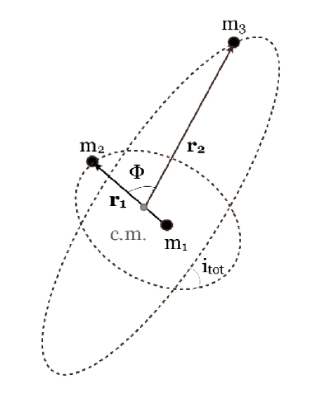
Figure 1: Coordinate system used to describe the hierarchical triple system (not to scale). Here ’c.m.’ denotes the center of mass of the inner binary, containing objects of masses $m_{1}$ and $m_{2}$. The separation vector ${\bf r}_{1}$ points from $m_{1}$ to $m_{2}$; ${\bf r}_{2}$ points from ’c.m.’ to $m_{3}$. The angle between the vectors ${\bf r}_{1}$ and ${\bf r}_{2}$ is $\Phi$.

We first define our basic notations. The system consists of a close binary (bodies of masses $m_{1}$ and $m_{2}$) and a third body (mass $m_{3}$). It is convenient to describe the orbits using Jacobi coordinates (Murray and Dermott, 2000, p. 441-443). Let ${\bf r}_{1}$ be the relative position vector from $m_{1}$ to $m_{2}$ and ${\bf r}_{2}$ the position vector of $m_{3}$ relative to the center of mass of the inner binary (see fig. 1). Using this coordinate system the dominant motion of the triple can be divided into two separate Keplerian orbits: the relative orbit of bodies 1 and 2, and the orbit of body 3 around the center of mass of bodies 1 and 2. The Hamiltonian for the system can be decomposed accordingly into two Keplerian Hamiltonians plus a coupling term that describes the (weak) interaction between the two orbits. Let the SMAs of the inner and outer orbits be $a_{1}$ and $a_{2}$, respectively. Then the coupling term in the complete Hamiltonian can be written as a power series in the ratio of the semi-major axes $\alpha=a_{1}/a_{2}$ (e.g., Harrington, 1968). In a hierarchical system, by definition, this parameter $\alpha$ is small.

The complete Hamiltonian expanded in orders of $\alpha$ is (e.g., Harrington, 1968),

$$\mathcal{H} = \frac{k^{2}m_{1}m_{2}}{2a_{1}}+\frac{k^{2}m_{3}(m_{1}+m_{2})}{2a_{2}}$$

$$+\frac{k^{2}}{a_{2}}\sum_{j=2}^{\infty}\alpha^{j}M_{j}\left(\frac{r_{1}}{a_{1}}\right)^{j}\left(\frac{a_{2}}{r_{2}}\right)^{j+1}P_{j}(\cos{\Phi})\ ,$$

where $k^{2}$ is the gravitational constant, $P_{j}$ are Legendre polynomials, $\Phi$ is the angle between ${\bf r}_{1}$ and ${\bf r}_{2}$ (see Figure 1) and

$$M_{j}=m_{1}m_{2}m_{3}\frac{m_{1}^{j-1}-(-m_{2})^{j-1}}{(m_{1}+m_{2})^{j}}\ .$$ (2)

Note that we have followed the convention of Harrington (1969) and chosen our Hamiltonian to be the negative of the total energy, so that $\mathcal{H}>0$ for bound systems.

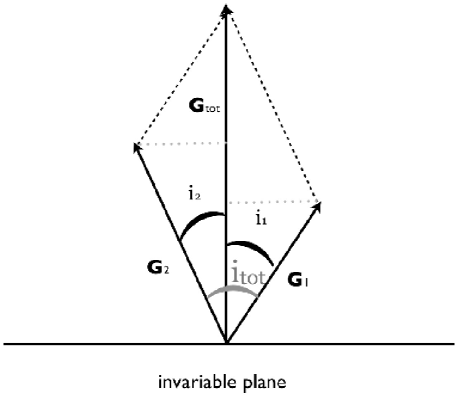
Figure 2: Geometry of the angular momentum vectors. We show the total angular momentum vector (${\bf G}_{\mathrm{tot}}$), the angular momentum vector of the inner orbit (${\bf G}_{1}$) with inclination $i_{1}$ with respect to ${\bf G}_{\mathrm{tot}}$ and the angular momentum vector of the outer orbit (${\bf G}_{2}$) with inclination $i_{2}$ with respect to ${\bf G}_{\mathrm{tot}}$. The angle between ${\bf G}_{1}$ and ${\bf G}_{2}$ defines the mutual inclination $i_{\mathrm{tot}}=i_{1}+i_{2}$. The invariable plane is perpendicular to ${\bf G}_{\mathrm{tot}}$.

We adopt the canonical variables known as Delaunay’s elements, which provide a particularly convenient dynamical description of our three-body system (e.g. Valtonen and Karttunen, 2006). The coordinates are chosen to be the mean anomalies, $l_{1}$ and $l_{2}$, the longitudes of ascending nodes, $h_{1}$ and $h_{2}$, and the arguments of periastron, $g_{1}$ and $g_{2}$, where subscripts $1,\,2$ denote the inner and outer orbits, respectively. Their conjugate momenta are

$$L_{1} = \frac{m_{1}m_{2}}{m_{1}+m_{2}}\sqrt{k^{2}(m_{1}+m_{2})a_{1}}\ ,$$ (3)

$$L_{2} = \frac{m_{3}(m_{1}+m_{2})}{m_{1}+m_{2}+m_{3}}\sqrt{k^{2}(m_{1}+m_{2}+m_{3})a_{2}}\ ,$$

$$G_{1}=L_{1}\sqrt{1-e_{1}^{2}}\ ,\quad G_{2}=L_{2}\sqrt{1-e_{2}^{2}}\ ,$$ (4)

and

$$H_{1}=G_{1}\cos{i_{1}}\ ,\quad H_{2}=G_{2}\cos{i_{2}}\ ,$$ (5)

where $e_{1}$ ($e_{2}$) is the inner (outer) orbit eccentricity. Note that $G_{1}$ and $G_{2}$ are also the magnitudes of the angular momentum vectors (${\bf G}_{1}$ and ${\bf G}_{2}$), and $H_{1}$ and $H_{2}$ are the $z$-components of these vectors. Figure 2 shows the resulting configuration of theses vectors. The following geometric relations between the momenta follow from the law of cosines:

$$\cos{i_{\textnormal{tot}}} = \frac{G_{\mathrm{tot}}^{2}-G_{1}^{2}-G_{2}^{2}}{2G_{1}G_{2}}\ ,$$ (6)

$$H_{1} = \frac{G_{\mathrm{tot}}^{2}+G_{1}^{2}-G_{2}^{2}}{2G_{\mathrm{tot}}}\ ,$$ (7)

$$H_{2} = \frac{G_{\mathrm{tot}}^{2}+G_{2}^{2}-G_{1}^{2}}{2G_{\mathrm{tot}}}\ ,$$ (8)

where ${\bf G}_{\mathrm{tot}}={\bf G}_{1}+{\bf G}_{2}$ is the (conserved) total angular momentum, and the angle between $\bf{G}_{1}$ and $\bf{G}_{2}$ defines the mutual inclination $i_{\mathrm{tot}}=i_{1}+i_{2}$. From eqs. (7) and (8) we find that the inclinations $i_{1}$ and $i_{2}$ are determined by the orbital angular momenta:

$$\cos i_{1} = \frac{G_{\mathrm{tot}}^{2}+G_{1}^{2}-G_{2}^{2}}{2G_{\mathrm{tot}}G_{1}}\ ,$$ (9)

$$\cos i_{2} = \frac{G_{\mathrm{tot}}^{2}+G_{2}^{2}-G_{1}^{2}}{2G_{\mathrm{tot}}G_{2}}\ .$$ (10)

In addition to these geometrical relations we also have that

$$H_{1}+H_{2}=G_{\mathrm{tot}}={\rm const}\ .$$ (11)

The canonical relations give the equations of motion:

$$\frac{dL_{j}}{dt}=\frac{\partial\mathcal{H}}{\partial l_{j}}\ ,\quad\frac{dl_{j}}{dt}=-\frac{\partial\mathcal{H}}{\partial L_{j}}\ ,$$ (12)

$$\frac{dG_{j}}{dt}=\frac{\partial\mathcal{H}}{\partial g_{j}}\ ,\quad\frac{dg_{j}}{dt}=-\frac{\partial\mathcal{H}}{\partial G_{j}}\ ,$$ (13)

$$\frac{dH_{j}}{dt}=\frac{\partial\mathcal{H}}{\partial h_{j}}\ ,\quad\frac{dh_{j}}{dt}=-\frac{\partial\mathcal{H}}{\partial H_{j}}\ ,$$ (14)

where $j=1,2$. Note that these canonical relations have the opposite sign relative to the usual relations (e.g., Goldstein, 1950) because of the sign convention we have chosen for our Hamiltonian. Finally we write the Hamiltonian through second order in $\alpha$ as (e.g., Kozai, 1962)

$$\mathcal{H} = \frac{\beta_{1}}{2L_{1}^{2}}+\frac{\beta_{2}}{2L_{2}^{2}}+$$

$$4\beta_{3}\left(\frac{L_{1}^{4}}{L_{2}^{6}}\right)\left(\frac{r_{1}}{a_{1}}\right)^{2}\left(\frac{a_{2}}{r_{2}}\right)^{3}\left(3\cos 2\Phi+1\right)\ ,$$

where the mass parameters are

$$\beta_{1} = k^{2}m_{1}m_{2}\frac{L_{1}^{2}}{a_{1}}\ ,$$ (16)

$$\beta_{2} = k^{2}(m_{1}+m_{2})m_{3}\frac{L_{2}^{2}}{a_{2}}$$ (17)

$$\quad{\rm and}$$

$$\beta_{3} = \frac{k^{4}}{16}\frac{\left(m_{1}+m_{2}\right)^{7}m_{3}^{7}}{\left(m_{1}m_{2}\right)^{3}\left(m_{1}+m_{2}+m_{3}\right)^{3}}\ .$$ (18)

3 Secular Evolution to the Quadrupole Order

In this section, we derive the secular quadrupole–level Hamiltonian. in Appendix A we develop the complete quadrupole-level secular approximation and in particular in Appendix A.3 we present the quadrupole–level equations of motion. The main difference between the derivation shown here (see also Appendix A) and those of previous studies lies in the “elimination of nodes” (e.g., Kozai, 1962; Jefferys and Moser, 1966). This is related to the transition to a coordinate system with the total angular momentum along the z-axis, which is known as the invariable plane (e.g., Murray and Dermott, 2000). In this coordinate system (see Figure 2), the longitudes of the ascending nodes differ by $\pi$, i.e.,

$$h_{1}-h_{2}=\pi\ .$$ (19)

Conservation of the total angular momentum implies that this relation holds at all times. Many previous works have exploited it to explicitly simplify the Hamiltonian by setting $h_{1}-h_{2}=\pi$ before deriving the equations of motion. After the substitution, the Hamiltonian is independent of the longitudes of ascending nodes ($h_{1}$ and $h_{2}$), and this can lead to the incorrect conclusion that $\dot{H}_{1}=\dot{H}_{2}=0$ when the canonical equations of motion are derived. Some previous studies incorrectly concluded that the $z$-components of the orbital angular momenta are always constant (see also Appendix C). The substitution $h_{1}-h_{2}=\pi$ is incorrect at the Hamiltonian level because it unduly restricts variations in the trajectory of the system to those where $\delta h_{1}=\delta h_{2}$. After deriving the equations of motion, however, we can exploit the relation $h_{1}-h_{2}=\Delta h=\pi$, which comes from the conservation of angular momentum. This considerably simplifies the evolution equations. We show (Appendices A.3 and B) that one can still use the Hamiltonian with the nodes eliminated found in previous studies (e.g., Kozai, 1962; Harrington, 1969) as long as the evolution equations for the inclinations are derived from the total angular momentum conservation, instead of using the canonical relations. Of course, the correct evolution equations can also be calculated from the correct Hamiltonian (without the nodes eliminated), which we derive in this section.

We note that there are some other derivations of the secular evolution equations that avoid the elimination of the nodes (Farago and Laskar, 2010; Laskar and Boué, 2010; Mardling, 2010; Katz and Dong, 2011), and thus do not suffer from this error.

The secular Hamiltonian is given by the average over the rapidly-varying $l_{1}$ and $l_{2}$ in equation (2) (see Appendix A for more details)

$$\mathcal{H}_{2} = \frac{C_{2}}{8}\big{\{}[1+3\cos(2i_{2})]\big{(}[2+3e_{1}^{2}][1+3\cos(2i_{1})]$$

$$+ 30e_{1}^{2}\cos(2g_{1})\sin^{2}(i_{1})\big{)}+3\cos(2\Delta h)[10e_{1}^{2}\cos(2g_{1})$$

$$\times \{3+\cos(2i_{1})\}+4(2+3e_{1}^{2})\sin(i_{1})^{2}]\sin^{2}(i_{2})$$

$$+ 12\{2+3e_{1}^{2}-5e_{1}^{2}\cos(2g_{1})\}\cos(\Delta h)\sin(2i_{1})\sin(2i_{2})$$

$$+ 120e^{2}_{1}\sin(i_{1})\sin(2i_{2})\sin(2g_{1})\sin(\Delta h)$$

$$- 120e_{1}^{2}\cos(i_{1})\sin^{2}(i_{2})\sin(2g_{1})\sin(2\Delta h)\big{\}}\ ,$$

where

$$C_{2}=\frac{k^{4}}{16}\frac{(m_{1}+m_{2})^{7}}{(m_{1}+m_{2}+m_{3})^{3}}\frac{m_{3}^{7}}{(m_{1}m_{2})^{3}}\frac{L_{1}^{4}}{L_{2}^{3}G_{2}^{3}}\ .$$ (21)

Making the usual (incorrect) substitution $\Delta h\to\pi$ (i.e. eliminating the nodes), we get the quadrupole-level Hamiltonian that has appeared in many previous works (see, e.g. Ford et al., 2000a):

$$\mathcal{H}_{2}(\Delta h\to\pi) = C_{2}\{\left(2+3e_{1}^{2}\right)\left(3\cos^{2}i_{\mathrm{tot}}-1\right)$$

$$+ 15e_{1}^{2}\sin^{2}i_{\mathrm{tot}}\cos(2g_{1})\}\ ,$$

where we have set $i_{1}+i_{2}=i_{\mathrm{tot}}$. Because this Hamiltonian is missing the longitudes of ascending nodes ($h_{1}$ and $h_{2}$), many previous studies concluded that the $z$-components (i.e. vertical components) of the angular momenta of the inner and outer orbits (i.e., $H_{1}$ and $H_{2}$) are constants.

We derive the quadrupole–level equations of motions in Appendix A.3. In particular, we give the equations of motion of the z-component of the angular momentum of the inner and outer orbits derived from the Hamiltonian in Eq. (3). As we show in the subsequent sections the evolution of $H_{1,2}$ produces a qualitatively different evolutionary route for many astrophysical systems considered in previous works.

In Appendix A.4 we show that the quadrupole approximation leads to well-defined minimum and maximum eccentricity and inclination. The eccentricity of the inner orbit and the inner (and mutual) inclination oscillate. In the test-particle limit, our formalism gives the critical initial mutual inclination angles for large oscillations of $39.2^{\circ}\leq i_{\textnormal{tot}}\leq 140.8^{\circ}$ with nearly-zero initial inner eccentricity, in agreement with Kozai (1962).

It is easy to show that $H_{1}$ and $H_{2}$ are constant only in the TPQ limit without using the explicit equations of motion in Appendix A. Because the Hamiltonian in Eq. (3) is independent of $g_{2}$, $G_{2}=\mathrm{const}$ at the quadrupole level. Combining this with the geometric relation in Eq. (7), $H_{1}=(G_{\rm tot}^{2}+G_{1}^{2}-G_{2}^{2})/(2G_{\rm tot})$, and the constantcy of the total angular momentum, $G_{\rm tot}$, we have that

$$\dot{H}_{1}=\frac{\dot{G}_{1}G_{1}}{G_{\mathrm{tot}}}.$$ (23)

In the TPQ limit, $G_{\mathrm{tot}}\gg G_{1}$, so $\dot{H}_{1}=-\dot{H}_{2}\approx 0$, and the $z$-component of each orbit’s angular momentum is conserved. Outside this limit, when $G_{1}/G_{\mathrm{tot}}$ is not negligable, $H_{1}$ and $H_{2}$ cannot be constant. Note that the TPQ limit, where $G_{1}\ll G_{\mathrm{tot}}$, is equivalent to the limit where $i_{2}\approx 0$ appearing in many previous works.

4 Octupole-Level Evolution

In Appendix B, we derive the secular evolution equations to octupole order. Many previous octupole–order derivations provided correct secular evolution equations for at least some of the elements, in spite of using the elimination of nodes substitution at the Hamiltonian level (e.g. Harrington, 1968, 1969; Sidlichovsky, 1983; Krymolowski and Mazeh, 1999; Ford et al., 2000a; Blaes et al., 2002; Lee and Peale, 2003; Thompson, 2011). This is because the evolution equations for $e_{2}$, $g_{2}$, $g_{1}$ and $e_{1}$ can be found correctly from a Hamiltonian that has had $h_{1}$ and $h_{2}$ eliminated by the relation $h_{1}-h_{2}=\pi$; the partial derivatives with respect to the other coordinates and momenta are not affected by the substitution. The correct evolution of $H_{1}$ and $H_{2}$ can then be derived, not from the canonical relations, but from total angular momentum conservation. We discuss in more details the comparison between this work and previous analyses in §5.

The octupole-level terms in the Hamiltonian can become important when the eccentricity of the outer orbit is non-zero, and if $\alpha$ is large enough. We quantify this by considering the ratio between the octupole to quadrupole-level coefficients, which is

$$\frac{C_{3}}{C_{2}}=\frac{15}{4}\left(\frac{m_{1}-m_{2}}{m_{1}+m_{2}}\right)\left(\frac{a_{1}}{a_{2}}\right)\frac{1}{1-e_{2}^{2}}\ ,$$ (24)

where $C_{3}$ is the octupole-level coefficient [eq. (71)] and $C_{2}$ is the quadrupole-level coefficient [eq. (21)]. We define

$$\epsilon_{M}=\left(\frac{m_{1}-m_{2}}{m_{1}+m_{2}}\right)\left(\frac{a_{1}}{a_{2}}\right)\frac{e_{2}}{1-e_{2}^{2}}\ ,$$ (25)

which gives the relative significance of the octupole-level term in the Hamiltonian. This parameter has three important parts; first the eccentricity of the outer orbit ($e_{2}$), second, the mass difference of the inner binary ($m_{1}$ and $m_{2}$) and the SMA ratio. In the test particle limit (i.e., $m_{1}\gg m_{2}$) $\epsilon_{M}$ is reduced to the octupole coefficient introduced in Lithwick and Naoz (2011) and Katz et al. (2011),

$$\epsilon=\left(\frac{a_{1}}{a_{2}}\right)\frac{e_{2}}{1-e_{2}^{2}}\ .$$ (26)

We call the octupole-level behavior of a system for which $\epsilon_{M}\ll 1$ is not satisfied the “eccentric Kozai-Lidov” (EKL) mechanism.

The octupole terms vanish when $e_{2}=0$. Therefore if one artificially held $e_{2}=0$, in the test-particle limit the inner body’s orbit would be given by the equations derived by Kozai (1962), i.e. by the test particle quadrupole equations. However, at octupole order the value of $e_{2}$ evolves in time if the inner body is massive. Furthermore, even if the inner body is massless, if the outer body has $e_{2}>0$ then the inner body’s behavior will also be different than in Kozai’s treatment. For example, Lithwick and Naoz (2011) and Katz et al. (2011) find that the inner orbit can flip orientation (see below) even in the test-particle, octupole limit. The octupole-level effects can change qualitatively the evolution of a system. Compared to the quadrupole-level behavior, the eccentricity of the inner orbit in the EKL mechanism can reach a much higher value. In some cases these excursions to very high eccentricities are accompanied by a “flip” of the orbit with respect to the total angular momentum, i.e. starting with $i_{1}<90^{\circ}$ the inner orbit can eventually reach $i_{1}>90^{\circ}$ (see Figures 6–9 for examples). Chaotic behavior is also possible at the octupole level (Lithwick and Naoz, 2011), but not at the quadrupole–level.

Given the large, qualitative changes in behavior moving from quadrupole to octupole order in the Hamiltonian, is it possible that similar changes in the secular evolution may occur at even higher orders? The answer to this question probably lies in the elimination of $G_{2}$ as an integral of motion at octupole order, leaving only four integrals of motion: the energy of the system, and the three components of the total angular momentum. There are no more integrals of motion to be eliminated, and thus one might expect no more dramatic changes in the evolution when moving to even higher orders. It is possible to see this quantitatively for specific initial conditions through comparisons with direct $n$-body integrations. We compared our octupole equations with direct $n$-body integrations, using the Mercury software package (Chambers and Migliorini, 1997). We used both Burlisch-Stoer and symplectic integrators (Wisdom and Holman, 1991) and found consistent results between the two. We present the results of a typical integration compared to the integration of the octupole-level secular equations in Figure 3. The initial conditions (see caption) for this system are those of Naoz et al. (2011), Figure 1. We find good agreement between the direct integration and the secular evolution at octupole order. Both show a beat-like pattern of eccentricity oscillations, suggesting an interference between the quadrupole and octupole terms, and both methods show similar flips of the inner orbit.

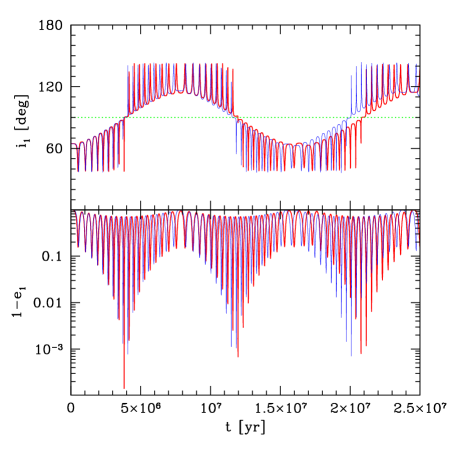
Figure 3: Comparison between a direct integration (using a B-S integrator) and the octupole-level approximation (see Appendix B). The red lines are from the integration of the octupole-level perturbation equations, while the blue lines are from the direct numerical integration of the three-body system. Here the inner binary contains a star of mass $1\,M_{\odot}$ and a planet of mass $1\,M_{\rm J}$, while the outer object is a brown dwarf of mass $40\,M_{\rm J}$. The inner orbit has $a_{1}=6\,$AU and the outer orbit has $a_{2}=100\,$AU. The initial eccentricities are $e_{1}=0.001$ and $e_{2}=0.6$ and the initial relative inclination $i_{\mathrm{tot}}=65^{\circ}$. The thin horizontal line in the top panel marks the $90^{\circ}$ boundary, separating prograde and retrograde orbits. The initial mutual inclination of $65^{\circ}$ corresponds to an inner and outer inclination with respect to the total angular momentum (parallel to z) of $64.7^{\circ}$ and $0.3^{\circ}$, respectively. Here, the arguments of pericenter of the inner orbit is set to $g_{1}=45^{\circ}$ and the outer orbit set to zero initially. The SMA of the two orbits (not shown) are nearly constant during the direct integration, varying by less than $0.02$ percent. The agreement in both period and amplitude of oscillation between the direct integration and the octupole-level approximation is quite good.

5 Implications and Comparison with Previous Studies

The Kozai (1962) and Lidov (1962) equations of motions are correct to quadrupole order and for a test particle, but differ from the correct evolution equations for non-test-particle inner orbits and/or at octupole order. In this Section we show how these differences give rise to qualitatively different evolutionary behaviors than those assumed in some previous works.

5.1 Massive Inner Object at the Quadrupole Level

The danger with working in the wrong limit is apparent if we consider an inner object that is more massive then the outer object. While the TPQ formalism incorrectly assumes that the orbit of the outer body is fixed in the invariable plane, and therefore the inner body’s vertical angular momentum is constant, the quadrupole-level equations presented in Appendix A.3 do not.

We compare the two formalisms in Figure 4. We consider the triple system PSR B1620$-$26 located near the core of the globular cluster M4. The inner binary contains a millisecond radio pulsar of $m_{1}=1.4M_{\odot}$ and a companion of $m_{2}=0.3M_{\odot}$ (McKenna and Lyne, 1988). Following Ford et al. (2000b), we adopt parameters for the outer perturber of $m_{3}=0.01\,M_{\odot}$ and $e_{2}=0$. Note that Ford et al. (2000b) found $e_{2}=0.45$, but it is interesting to show that even for an axisymmetric outer potential the evolution of the system is qualitatively different then the TPQ approximation (see the caption for a full description of the initial conditions). Note that the actual measured inner binary eccentricity is $e_{1}\sim 0.045$, however in order to illustrate the difference we adopt a higher value ($e_{1}=0.5$ ). For these initial conditions $\epsilon_{M}=0.036$, so a careful analysis would require incorporating the octupole–order terms in the motion; nevertheless, we consider the evolution of the system to quadrupole order for comparison with the TPQ formalism. We have verified, however, that the neglected octupole–order effects do not qualitatively change the behavior of the system. This is because the outer companion mass is low, and hence the inner orbit does not exhibit large amplitude oscillations.

For the comparison, we do not compare the (constant) $H_{1}$ from the TPQ formalism to the (varying) $H_{1}$ of the correct formalism. Instead, we compare the (varying) $H_{1}$ from the correct formalism (solid red line) with $G_{1}\cos i_{\mathrm{tot}}$ (dashed blue line), which is the vertical angular momentum that would be inferred in our formalism if the outer orbit were instantaneously in the invariable plane, as assumed in the TPQ formalism.

In Figure 4, the mutual inclination oscillates between $106.7^{\circ}$ to $57.5^{\circ}$, and thus crosses $90^{\circ}$. These oscillations are mostly due to the oscillations of the outer orbit’s inclination, while $i_{1}$ does not change by more than $\sim 1^{\circ}$ in each cycle. Clearly, the outer orbit does not lie in the fixed invariable plane. Figure 4, bottom panel, shows $\sqrt{1-e_{1}^{2}}\cos i_{\mathrm{tot}}$, which, in the TPQ limit, is the vertical angular momentum of the inner body.

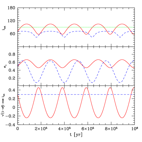
Figure 4: Comparison between the standard TPQ formalism (dashed blue lines) and our method (solid red lines) for the case of PSR B1620$-$26. Here the inner binary is a millisecond pulsar of mass $1.4\,M_{\odot}$ with a companion of $m_{2}=0.3M_{\odot}$, and the outer body has mass $m_{3}=0.01M_{\odot}$. The inner orbit has $a_{1}=5\,$AU and the outer orbit has $a_{2}=50\,$AU (Ford et al., 2000b). The initial eccentricities are $e_{1}=0.5$ and $e_{2}=0$ and the initial relative inclination $i_{\mathrm{tot}}=70^{\circ}$. The thin horizontal line in the top panel marks the $90^{\circ}$ boundary, separating prograde and retrograde orbits. The initial mutual inclination of $70^{\circ}$ corresponds to an inner and outer inclination with respect to the total angular momentum (parallel to $\hat{\mathbf{z}}$) of $6.75^{\circ}$ and $63.25^{\circ}$, respectively. The argument of pericenter of the inner orbit is initially set $120^{\circ}$, while the outer orbit’s is set to zero. We consider, from top to bottom, the mutual inclination $i_{\mathrm{tot}}$, the inner orbit’s eccentricity and $\sqrt{1-e_{1}^{2}}\cos i_{\mathrm{tot}}$, which the standard formalism assumes to be constant (dashed line).

We can evaluate analytically the error introduced by the application of the TPQ formalism to this situation. We compare the vertical angular momentum ($H_{1}$) as calculated here to $H_{1}^{TPQ}=L_{1}\sqrt{1-e_{1}^{2}}\cos i={\rm const.}$. The relative error between the formalisms is $H_{1}^{TPQ}/H_{1}-1$. In Figure 5 we show the ratio between the inner orbit’s vertical angular momentum in the TPQ limit (i.e., $H_{1}^{TPQ}=G_{1}\cos i$) and equation (52) as a function of the total angular momentum ratio, $G_{1}/G_{2}$, for various inclinations. Note that this error can be calculated without evolving the system by using angular momentum conservation, Eq. (6). The TPQ limit is only valid when $G_{1}/G_{2}\mathrel{\hbox to0.0pt{\lower 4.0pt\hbox{\hskip 1.0pt$\sim$}\hss}\raise 1.0pt\hbox{$<$}}10^{-4}$.

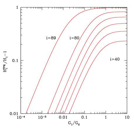
Figure 5: The ratio between the correct, changing $z$-component of the angular momentum, $H_{1}$, and the TPQ assumption often used in the literature, $H_{1}^{TPQ}=G_{1}\cos i_{\mathrm{tot}}$. This ratio was calculated analytically for various total angular momentum ratios, $G_{1}/G_{2}$, and inclinations. The curves, from bottom to top, have $i=40,50,60,70,80$ and $89$ degrees.

5.2 Octupole–Level Planetary Dynamics

Recent measurements of the sky-projected angle between the orbits of several hot Jupiters and the spins of their host stars have shown that roughly one in four is retrograde (Gaudi and Winn, 2007; Triaud et al., 2010; Albrecht et al., 2012). If these planets migrated in from much larger distances through their interaction with the protoplanetary disk (Lin and Papaloizou, 1986; Masset and Papaloizou, 2003), their orbits should have low eccentricities and inclinations. Disk migration scenarios therefore have difficulty accounting for the observed retrograde hot Jupiter orbits. An alternative migration scenario that can account for the retrograde orbits is the secular interaction between a planet and a binary stellar companion (Wu and Murray, 2003; Fabrycky and Tremaine, 2007; Wu et al., 2007; Takeda et al., 2008; Correia et al., 2011). For an extremely distant and massive companion ($\epsilon_{M}\to\epsilon\ll 1$) the quadrupole test-particle approximation applies, and $\sqrt{1-e_{1}^{2}}\cos i_{1}$ is nearly constant (where the planet is the massless body). Although this forbids orbits that are truly retrograde (with respect to the total angular momentum of the system), if the inner orbit begins highly inclined relative to the outer star’s orbit and aligned with the spin of the inner star, then the star-planet spin-orbit angle can change by more than $90^{\circ}$ during the secular evolution of the system, producing apparently retrograde orbits (Fabrycky and Tremaine, 2007; Correia et al., 2011). Nonetheless, a difficulty with this “stellar Kozai” mechanism is that even with the most optimistic assumptions it can only produce $\mathrel{\hbox to0.0pt{\lower 4.0pt\hbox{\hskip 1.0pt$\sim$}\hss}\raise 1.0pt\hbox{$<$}}10\%$ of hot Jupiters (Wu et al., 2007).

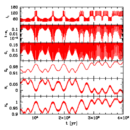
Figure 6: Evolution of a planetary system with $m_{1}=1\,M_{\odot}$, $m_{2}=1\,M_{J}$ and $m_{3}=2\,M_{J}$, with $a_{1}=4$ AU and $a_{2}=45$ AU. We initialize the system at $t=0$ with $e_{1}=0.01$, $e_{2}=0.6$, $g_{1}=180^{\circ}$, $g_{2}=0^{\circ}$ and $i_{\textnormal{tot}}=67^{\circ}$. For these initial conditions $i_{1}=57.92^{\circ}$ and $i_{2}=9.08^{\circ}$. The $z$-components of the orbital angular momenta, $H_{1}$ and $H_{2}$, are shown normalized to the total angular momentum of each orbit. The inner orbit flips repeatedly between prograde ($i_{1}<90^{\circ}$) and retrograde ($i_{1}>90^{\circ}$).

Figure 7: Zoom-in on part of the evolution of the point-mass planetary system in Figure 6. In this zoom-in, we can see that flips in the inner orbit—$i_{1}$ crossing $90^{\circ}$—are associated with excursions to very high eccentricity.

Wu and Murray (2003), Wu et al. (2007), Fabrycky and Tremaine (2007) and Correia et al. (2011) studied the evolution of a Jupiter-mass planet in stellar binaries in the TPQ formalism. For example, the case of HD 80606b (Wu and Murray (2003, Fig. 1); Fabrycky and Tremaine (2007, Fig. 1) and Correia et al. (2011, also Fig. 1)) was considered with an outer stellar companion at $1000$ AU. However, if the companion is assumed to be eccentric $\epsilon_{M}$ is not negligible, and the system is more appropriately described with the test particle octupole–level approximation (e.g., Lithwick and Naoz, 2011; Katz et al., 2011). Furthermore, the statistical distribution for closer stellar binaries in Wu et al. (2007) and Fabrycky and Tremaine (2007) is only valid in the approximation where the outer orbit’s eccentricity is zero. In fact, for the systems considered in those studies $\epsilon_{M}$ is not negligible and the octupole–level approximation results in dramatically different behavior as was shown in Naoz et al. (2012a). The same dramatic difference in behavior also exists in the analysis of triple stars (e.g., Fabrycky and Tremaine, 2007; Perets and Fabrycky, 2009), see §5.4.

A dramatic difference between the octupole and quadrupole–level of approximation is that the former often generates extremely high eccentricities. In real systems, such high eccentricities can be suppressed by tides or GR (e.g., Söderhjelm, 1984; Eggleton et al., 1998; Kiseleva et al., 1998; Borkovits et al., 2004). Flips can also be prevented because they typically occur shortly after extreme eccentricities (see Teyssandier et al. in prep.). In our previous studies that include tides, planetary perturbers typically allow flips to happen, while stellar perturbers mostly suppress them (Naoz et al., 2011, 2012a) But in both cases, tides quantitatively affect the evolution.

Naoz et al. (2011) considered planet-planet secular interactions with tidal interactions as a possible source of retrograde hot Jupiters. In this situation $\epsilon_{M}$ is not small, requiring computation of the octupole-level secular dynamics. In Figures 6 and 7 we show the evolution of a representative configuration (see the caption for a full description of the initial conditions). For this configuration, $\epsilon_{M}=0.083$. Flips of the inner orbit are associated with evolution to very high eccentricity (see Figures 6 and 7).

5.3 Octupole–Level Solar System Dynamics

Kozai (1962) studied the dynamical evolution of an asteroid due to Jupiter’s secular perturbations. He assumed that Jupiter’s eccentricity is strictly zero. However, Jupiter’s eccentricity is $\sim 0.05$, and thus studying the evolution of a test particle in the asteroid belt ($a_{1}\sim 2-3$ AU) places the evolution in a regime where the eccentric Kozai-Lidov effect could be significant, with $\epsilon_{M}=\epsilon=0.03$ (Lithwick and Naoz, 2011; Katz et al., 2011).

We considered the evolution of asteroid at $2$ AU (assumed to be a test particle) due to Jupiter at $5$ AU with eccentricity of $e_{2}=0.05$ (see the caption for a full description of the initial conditions). The asteroid is a test particle and therefore $i_{1}\approx i_{\mathrm{tot}}$. In Figure 8 we compare the evolution of an asteroid using the TPQ limit (e.g., Kozai, 1962; Thomas and Morbidelli, 1996; Kinoshita and Nakai, 2007) and the octupole-level evolution discussed here. For this value of $\epsilon$, the eccentric Kozai-Lidov effect significantly alters the evolution of the asteroid, even driving it to such high inclination that the orbit becomes retrograde. Though we deal only with point masses in this work, note that the eccentricity is so high that the inner orbit’s pericenter lies well within the sun.

The value of $\epsilon$ here is mainly due to the relative high $\alpha$ in the problem (an issue raised in the original work on this problem (Kozai, 1962)). The system is very packed which raises questions with regards to the validity of the hierarchical approximation. Even in the EKL formalism, such high eccentricities occur that the asteriod collides with the sun and the apo-center of the asteroid approaches about $1$ AU from Jupiter’s orbit. To determine the importance of these effects, we ran an $N$-body simulation using the Mercury software package (Chambers and Migliorini, 1997). We used both Bulirsch-Stoer and symplectic integrators (Wisdom and Holman, 1991). The results are depicted at Figure 8, which show that the TPQ limit is indeed inadequate for the system. In addition the octupole–level approximation has some deviations from the direct $N$-body integration, particularly in the high eccentricity regime. Note that the evolution of the asteroid in the direct integration resulted in a collision with the Sun. In reality, it is likely that a planetary encounter would remove the asteroid from the solar system before this point. In contrast to the EKL mechanism, assuming zero eccentricity for Jupiter results in consistent results between the secular evolution and the direct integration (Thomas and Morbidelli, 1996).

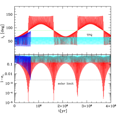
Figure 8: Evolution of an asteroid due to Jupiter’s secular gravitational perturbations (Kozai 1962). We consider $m_{1}=1\,M_{\odot}$, $m_{2}\to 0$ and $m_{3}=1$ M_J, with $a_{1}=2$ AU and $a_{2}=5$ AU. We initialize the system at $t=0$ with $e_{1}=0.2$, $e_{2}=0.05$, $g_{1}=g_{2}=0^{\circ}$ and $i_{\mathrm{tot}}=65^{\circ}$. We show the TPQ evolution (cyan lines) and the EKL evolution (red lines). The thin horizontal dotted line in the top panel marks the $90^{\circ}$ boundary, separating prograde and retrograde orbits. The inner orbit flips periodically between prograde ($i_{1}<90^{\circ}$) and retrograde ($i_{1}>90^{\circ}$). We also show the result of an $N$-body simulation (blue lines). The thin horizontal dotted line in the bottom panel marks the eccentricity corresponding to a collision with the solar surface, $1-e_{1}=R_{\odot}/a_{1}$.

As shown in Figure 8, taking into account Jupiter’s eccentricity ($\sim 0.05$), produces a dramatically different evolutionary behavior, including retrograde orbits for the asteroid. Thomas and Morbidelli (1996) applied the TPQ formalism to the asteroid-Jupiter setting (see for example their Figure 2 for $a_{1}=3$ AU). Kinoshita and Nakai (2007) developed an analytical solution for the TPQ limit (see also Kinoshita and Nakai, 1991, 1999).

The TPQ formalism has also been applied to the study of the outer solar system. Kinoshita and Nakai (2007) applied their analytical solution to Neptune’s outer satellite Laomedeia. This system has $\epsilon\to 0$ and thus the TPQ limit there is justified. In addition, Perets and Naoz (2009) have studied the evolution of binary minor planets using the TPQ approximation. In this problem $\epsilon\to 0$ and thus the TPQ approximation is valid.

Lidov and Ziglin (1976, sections 3–4) also solved analytically the quadrapole–level approximation but, unlike Kinoshita and Nakai (2007), they did not restrict themselves to the TPQ limit, and used the total angular momentum conservation law in order to calculate the inclinations. Thus, their formalism is equivalent to ours at quadrupole–order. Later, Mazeh and Shaham (1979) also derived evolution equations outside the TPQ limit (their eqs. A1-A8), allowing for small eccentricities and inclinations of the outer body.

5.4 Octupole–Level Perturbations in Triple Stars

The evolution of triple stars has been studied by many authors using the standard (TPQ) formalism (e.g., Mazeh and Shaham, 1979; Eggleton et al., 1998; Kiseleva et al., 1998; Mikkola and Tanikawa, 1998; Eggleton and Kiseleva-Eggleton, 2001; Fabrycky and Tremaine, 2007; Perets and Fabrycky, 2009). In some cases the corrected formalism derived here can give rise to qualitatively different results. We show that some of the previous studies should be repeated in order to account for the correct dynamical evolution, and give one example where the eccentric Kozi-Lidov mechanism dramatically changes the evolution.

Fabrycky and Tremaine (2007) studied the distribution of triple star properties using Monte Carlo simulations. We choose a particular system from their triple-star suite of simulations to illustrate how the dynamics including the octupole order can be qualitatively different from what would be seen at quadrupole order (see the caption for a full description of the initial conditions). For this system $\epsilon_{M}=0.042$ (and $\epsilon=0.0703$). The evolution of the system is shown in Figure 9. At octupole order, the inclination of the inner orbit oscillates between about $40^{\circ}$ and $140^{\circ}$, often becoming retrograde (relative to the total angular momentum), while the quadrupole–order behavior is very different and the inner orbit remains always prograde. The octupole–order treatment also gives rise to much higher eccentricities (Krymolowski and Mazeh, 1999; Ford et al., 2000a). In Figure 10 we compare the octupole–level evolution (of the same system) with direct 3–body integration.

The evolution shown in Figure 9 is for point-mass stars; in reality, these high-eccentricity excursions would actually drive the inner binary to its Roche limit, leading to mass transfer. For these high eccentricities tides will play an important role and thus in reality flips in similar systems may be suppressed. Similarly the high eccentricities often excited through the eccentric Kozai mechanism can also lead to compact object binary merger.

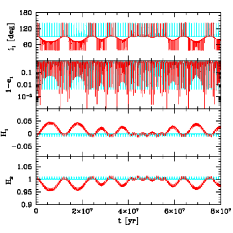
Figure 9: An example of dramatically different evolution between the quadruple and octupole approximations for a triple-star system. The system has $m_{1}=1M_{\odot}$, $m_{2}=0.25M_{\odot}$ and $m_{3}=0.6M_{\odot}$, with $a_{1}=60$ AU and $a_{2}=800$ AU. We initialize the system with $e_{1}=0.01$, $e_{2}=0.6$, $g_{1}=g_{2}=0^{\circ}$ and $i_{\mathrm{tot}}=98^{\circ}$, taken from Fabrycky and Tremaine (2007). For these initial conditions $i_{1}=90.02^{\circ}$ and $i_{2}=7.98^{\circ}$. We show both the (correct) quadrupole-level evolution (light-blue lines) and the octupole-level evolution (red lines). $H_{1}$ and $H_{2}$, the $z$-components of the angular momenta of the orbits, are normalized to the total angular momentum. Note that the octupole-level evolution produces periodic transitions from prograde to retrograde inner orbits (relative to the total angular momentum), while at the quadrupole-level the inner orbit remains prograde. See Figure 10 for comparison with direct numerical integration of the three-body system.

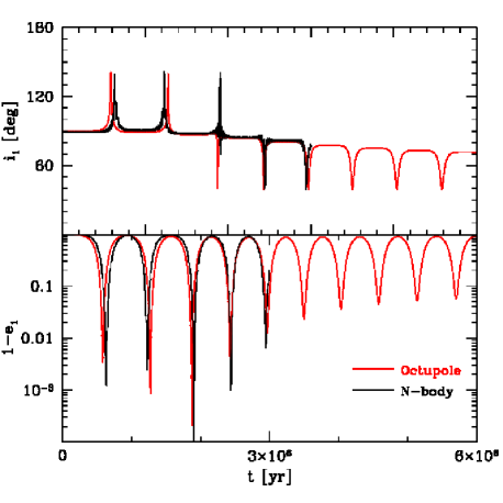
Figure 10: The evolution for the first $6$ Myr, of Figure 9 where we show a comparison between direct 3–body integration (using a B-S integrator), and the octupole–level of approximation. The red lines are from the integration of the octupole-level perturbation equations, while the black lines are from the direct numerical integration of the three-body system.

The possibility of forming blue stragglers through secular interactions in triple star systems has been suggested by Perets and Fabrycky (2009) and Geller et al. (2011). As shown in Krymolowski and Mazeh (1999); Ford et al. (2000a) and in the example above the minimum pericenter distance of the inner binary can differ significantly between the TPQ and EKL formalisms. This suggests that using the correct EKL formalism could significantly increase the computed likelihood of such a formation mechanism for blue stragglers.

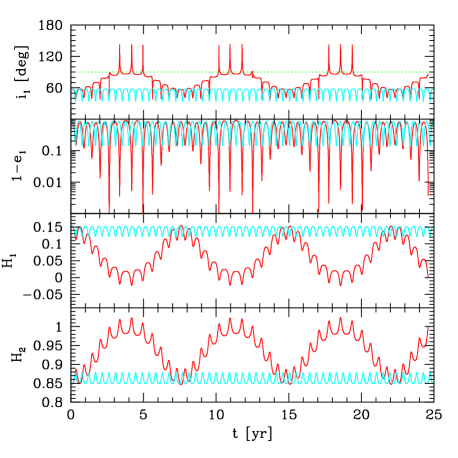
Figure 11: An example of dramatically different evolution between the quadruple and octupole approximations for a triple star system representing the best-fit parameters from the Mikkola and Tanikawa (1998) analysis of CH Cygni. The system has $m_{1}=3.51M_{\odot}$, $m_{2}=0.5M_{\odot}$ and $m_{3}=0.909M_{\odot}$, with $a_{1}=0.05$ AU and $a_{2}=0.21$ AU. We initialize the system with $e_{1}=0.32$, $e_{2}=0.6$, $g_{1}=145^{\circ}$, $g_{2}=0^{\circ}$ and $i_{\mathrm{tot}}=72^{\circ}$. For these initial conditions $i_{1}=57.02^{\circ}$ and $i_{2}=14.98^{\circ}$. We show both the (non-TPQ) quadrupole-level evolution (light-blue lines) and the octupole-level evolution (red lines). $H_{1}$ and $H_{2}$, the z-components of the angular momenta of the orbits, are normalized to the total angular momentum. Note that the octupole-level evolution produces periodic transitions from prograde to retrograde inner orbits (relative to the total angular momentum), while at the quadrupole-level the inner orbit remains prograde. To avoid clutter in the figure we have omitted the TPQ result. In the TPQ formalism, the evolution of the inclination and eccentricity are similar to the general quadrupole-level approximation, but $H_{1,2}$ are constant.

For many years CH Cygni was considered to be an interesting triple candidate because it exhibits two clear distinguishable periods (e.g. Donnison and Mikulskis, 1995; Skopal et al., 1998; Mikkola and Tanikawa, 1998; Hinkle et al., 1993). However, a triple system model based on the TPQ Kozai mechanism (Mikkola and Tanikawa, 1998) did not reproduce the observed masses of the system (Hinkle et al., 1993, 2009). Applying the corrected formalism in this paper to the system parameters derived in Mikkola and Tanikawa (1998) gives a very different evolution than in the TPQ formalism. Therefore, it seems likely that an analysis based on the formalism discussed in this paper would give a significantly different fit. In Figure 11 we illustrate the differences between the TPQ, correct quadrupole, and octupole evolution of the system. The best-fit parameters of the system are taken from Mikkola and Tanikawa (1998) where $\epsilon_{M}=0.14$ (see the caption for a full description of the initial conditions, where we allowed for a freedom in our choice of $e_{2},g_{1},g_{2}$ and $i_{\textnormal{tot}}$ since the best fit was found using the TPQ limit, at which $e_{2}$ is fixed). Note that the choice of the inner eccentricity does not strongly influence the evolution while the choice of the outer orbit’s eccentricity does. Most importantly, the rather large $\epsilon_{M}$ for this system implies that the system is not stable, i.e., the averaging over the orbits is not justified. From direct integration we found that the system undergoes strong encounters and the inner binary collides in this example.

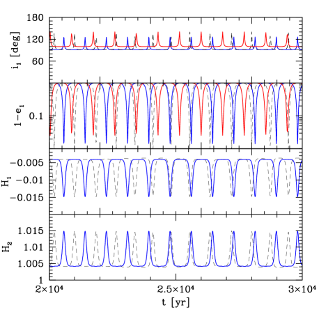
Figure 12: The time evolution of an Algol–like system (Eggleton et al., 1998), with $(m_{1},m_{2},m_{3})=(2.5,2,1.7)$ M_⊙. The inner orbit has $a_{1}=0.095\,$AU and the outer orbit has $a_{2}=2.777\,$AU. The initial eccentricities are $e_{1}=0.01$ and $e_{2}=0.23$ and the initial relative inclination $i_{\mathrm{tot}}=100^{\circ}$. The $z$-components of the inner and outer orbital angular momentum, $H_{1}$ and $H_{2}$ are normalized to the total angular momentum. The initial mutual inclination of $100^{\circ}$ corresponds to inner- and outer-orbit inclinations of $91.6^{\circ}$ and $8.4^{\circ}$, respectively. We consider the (correct) quadrupole-level evolution (blue lines), octupole-level evolution (dashed lines) and also the standard (incorrect) TPQ evolution. In the latter we have assumed, as in previous papers, that $i_{\mathrm{tot}}=i_{1}$, which results in the discrepancy between the inclination values. See also Figure 13 for the evolution of the Algol–like system using the updated masses and orbital parameter, following Baron et al. (2012).

It is also interesting to investigate a system for which the eccentric Kozai mechanism is suppressed due to comparable masses for the inner orbit, and low eccentricity of the outer orbit (i.e., $\epsilon_{M}<<1$). Kiseleva et al. (1998) and Eggleton and Kiseleva-Eggleton (2001) studied the Algol triple system (Lestrade et al., 1993) using the TPQ equations. The TPQ equations were also used in the paper that introduced the influential KCTF mechanism (Mazeh and Shaham, 1979; Eggleton et al., 1998). Note that tides dominate the evolution of the Algol system today (e.g.,  Söderhjelm, 2006). Figure 12 compares the evolution computed in the (incorrect) TPQ formalism, the correct quadrupole formalism, and the octupole-level EKL formalism applied to an Algol–like system. The correct quadrupole formalism decreases the minimum value of $1-e_{1}$ by almost a factor of 2 relative to the TPQ formalism. The reduced pericenter distance would strongly increase the effects of tidal friction (not included here), which may lead to rapid circularization of the inner orbit. The octupole-level computation decreases the minimum pericenter distance by a further 40%.

Note that the masses and orbital parameters used in Kiseleva et al. (1998) and Eggleton and Kiseleva-Eggleton (2001) are out of date. New observations (e.g., Baron et al., 2012) find the secondary mass to be smaller then the primary and the mutual inclination to be closer to $90^{\circ}$. In Figure 13 we show the octupole–level evolution of the system considering the new parameters. In the absence of any additional physical mechanism, such as general relativity, tides, mass transfer, etc., the EKL mechanism could play a very important role in the dynamical evolution of the system.

We note that the inner binary in the Algol system is dominated by tidal effects (Söderhjelm, 1975; Kiseleva et al., 1998; Eggleton and Kiseleva-Eggleton, 2001) and figures 12 and 13 do not represent the system today but an Algol–like analogy. We use the Algol parameters here only to show hypothetical outcomes of the correct dynamical evolution. It would be interesting to study stellar evolution including tides in the context of the EKL mechanism, for a system such as Algol.

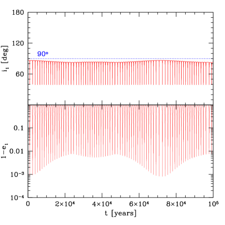
Figure 13: The time evolution of Algol–like system using the orbital parameters taken from Baron et al. (2012), with $(m_{1},m_{2},m_{3})=(3.17,0.7,1.7)$ M_⊙. The inner orbit has $a_{1}=0.062\,$AU and the outer orbit has $a_{2}=2.68\,$AU. The initial eccentricities are $e_{1}=0.001$ and $e_{2}=0.23$ and the initial relative inclination $i_{\mathrm{tot}}=90^{\circ}$. The initial mutual inclination of $90^{\circ}$ corresponds to inner- and outer-orbit inclinations of $86.4^{\circ}$ and $3.6^{\circ}$, respectively. We consider only the octupole-level evolution. Compare this to the evolution in Figure 12.

5.5 The Danger of the Quadrupole–Level of Approximation

The octupole-level Hamiltonian and equations of motion were previously derived by Harrington (1968, 1969); Sidlichovsky (1983); Marchal (1990); Krymolowski and Mazeh (1999); Ford et al. (2000a); Blaes et al. (2002) and Lee and Peale (2003). Most of the equations of motion can be derived correctly when applying the elimination of the nodes—only the $\dot{H}_{1}$ and $\dot{H}_{2}$ equations are affected. These authors calculated the time evolution of the inclinations (i.e. $H_{1}$ and $H_{2}$) from the total (conserved) angular momentum, and thus avoided the problem that arises when eliminating the nodes from the Hamiltonian. In appendix B we show the complete set of equations of motion for the octupole-level approximation, derived from a correct Hamiltonian, including the nodal terms.

As displayed here the octupole-level approximation gives rise to a qualitatively different evolutionary behavior for cases where $\epsilon_{M}$ [see eq. (25)] is not negligible. We note that many previous studies applied the quadrupole-level approximation, which may lead to significantly different results (e.g., Mazeh and Shaham, 1979; Quinn et al., 1990; Bailey et al., 1992; Innanen et al., 1997; Eggleton et al., 1998; Mikkola and Tanikawa, 1998; Eggleton and Kiseleva-Eggleton, 2001; Valtonen and Karttunen, 2006; Fabrycky and Tremaine, 2007; Wu et al., 2007; Zdziarski et al., 2007; Takeda et al., 2008; Perets and Fabrycky, 2009). Neglecting the octupole-level approximation can cause changes in the dynamics varying from a few percent to completely different qualitative behavior.

Some other derivations of octupole–order equations of motion dealt with the secular dynamics in a general way, without using Hamiltonian perturbation theory or elimination of the nodes (Farago and Laskar, 2010; Laskar and Boué, 2010; Mardling, 2010; Katz and Dong, 2011). In these works there were no references to the discrepancy between these derivations and the previous studies. Also, note that the results of Holman et al. (1997) are based on a direct N-body integration, and thus are not subject to the errors mentioned above.

6 Conclusions

We have shown that the “standard” TPQ Kozai formalism (Kozai, 1962; Lidov, 1962) has been applied in inappropriate situations. A common error in the implementation of the relevant Hamiltonian mechanics (premature elimination of the nodes) leads to the (incorrect) conclusion that the conservation of the $z$-component of each orbit’s angular momentum from the TPQ dynamics generalizes beyond the TPQ approximation. Correcting the formalism we find that the $z$-components of both the inner and outer orbits’ angular momenta in general change with time at both the quadrupole and octupole level. The conservation of the inner orbit’s $z$-component of the angular momentum (the famous $\sqrt{1-e_{1}^{2}}\cos i={\rm constant}$) only holds in the quadrupole-level test particle approximation. We have explained in details the source of the error in previous derivations (Appendix C).

We have re-derived the secular evolution equations for triple systems using Hamiltonian perturbation theory to the octupole-level of approximation (Section 2 and Appendix A, 4 and Appendix B). We have also shown that one can use the simplified Hamiltonian found in the literature (e.g., Ford et al., 2000a) as long as the equations of motion for the inclinations are calculated from the total angular momentum.

The correction shown here has important implications to the evolution of triple systems. We discussed a few interesting implications in Section 5. We showed that already at the quadrupole-level approximation the explicit assumption that the vertical angular momentum is constant can lead to erroneous results, see for example Figure 4. In this Figure we showed that far from the test particle limit in the quadrupole-level one can already find a significant difference in the evolutionary behavior. The correct results agree with the test particle limit only when $G_{1}/G_{2}<10^{-4}$ (see Figure 5). We show in Appendix A.4 that at the quadrupole level of approximation, the inner eccentricity and the mutual inclination have a well defined maximum and minimum irrespective of the mass of the inner bodies. In the test particle limit these values converge to the well-known critical inclinations ($39.2^{\circ}\leq i_{0}\leq 140.8^{\circ}$) for large oscillatory amplitudes.

The most notable outcome of the results presented here happens in the octupole-level of approximation (which we call the EKL formalism), when the inner orbit flips from prograde to retrograde with respect to the total angular momentum. Just before the flip the inner orbit has an excursion of extremely high eccentricity. In the presence of tidal forces (not included in this study) the outcome of a system can be different than the one assumed while using the TPQ formalism. Krymolowski and Mazeh (1999), Ford et al. (2000a), Blaes et al. (2002), Lee and Peale (2003) and Laskar and Boué (2010) present the correct octupole equations of motion. Had these authors integrated their equations for systems such as those presented in this paper, they could already have discovered the possibility of flipping the inner orbit.

Appendix A The Quadrupole level of Approximation

We develop the complete quadrupole-level secular approximation in this section. As mentioned, the main difference between the derivation shown here and those of previous studies lies in the “elimination of nodes” (e.g., Kozai, 1962; Jefferys and Moser, 1966), which relates to the transition the invariable plane (e.g., Murray and Dermott, 2000) coordinate system, where the total angular momentum lies along the $z$-axis.

A.1 Transformation to the Invariable Plane

We choose to work in a coordinate system where the total initial angular momentum of the system lies along the $z$ axis (see Figure 2),; the $x$-$y$ plane in this coordinate system is known as the invariable plane (e.g., Murray and Dermott, 2000), and therefore we call this coordinate system the invariable coordinate system. We begin by expressing the vectors ${\bf r}_{1}$ and ${\bf r}_{2}$ each in a coordinate system where the periapse of the orbit is aligned with the x-axis and the orbit lies in the x-y plane, called the “orbital coordinate system,” and then rotating each vector to the invariable coordinate system. The rotation that takes the position vector in the orbital coordinate system to the position in the invariable coordinate system is given by (see Murray and Dermott, 2000, chapter 2.8, and Figure 2.14 for more details)

$${\bf r}_{1,\textnormal{inv}}=R_{z}(h_{1})R_{x}(i_{1})R_{z}(g_{1}){\bf r}_{1,\textnormal{orb}}\ ,$$ (27)

where the subscript “inv” and “orb” refer to the invariable and orbital coordinate systems, respectively. The rotation matrices $R_{z}$ and $R_{x}$ as a function of rotation angle, $\theta$, are

$$R_{z}(\theta)=\left(\begin{array}[]{ccc}\cos\theta&-\sin\theta&0\\ \sin\theta&\cos\theta&0\\ 0&0&1\end{array}\right)$$ (28)

and

$$R_{x}(\theta)=\left(\begin{array}[]{ccc}1&0&0\\ 0&\cos\theta&-\sin\theta\\ 0&\sin\theta&\cos\theta\end{array}\right)\ .$$ (29)

Thus, the angle between ${\bf r}_{1}$ and ${\bf r}_{2}$ is given by:

$$\cos\Phi=\hat{{\bf r}}_{2,\textnormal{orb}}^{T}R^{-1}_{z}(g_{2})R^{-1}_{x}(i_{2})R_{z}^{-1}(h_{2})R_{z}(h_{1})R_{x}(i_{1})R_{z}(g_{1})\hat{{\bf r}}_{1,\textnormal{orb}},$$ (30)

where $\hat{{\bf r}}_{1,2,\textnormal{orb}}$ are unit vectors that point along ${\bf r}_{1,2,\textnormal{orb}}$. In the orbital coordinate system, we have

$$\hat{{\bf r}}_{1,2,\textnormal{orb}}=\begin{pmatrix}\cos\left(f_{1,2}\right)\\ \sin\left(f_{1,2}\right)\\ 0\end{pmatrix}\,,$$ (31)

where $f_{1}$ ($f_{2}$) is the true anomaly for the inner (outer) orbit. Note that $R_{z}^{-1}(h_{2})R_{z}(h_{1})=R_{z}(h_{1}-h_{2})\equiv R_{z}(\Delta h)$, so the Hamiltonian will depend on the difference in the longitudes of the ascending nodes; in a similar manner, the Hamiltonian depends on $f_{1}$ and $f_{2}$ only through expressions of the form $f_{1}+g_{1}$ and $f_{2}+g_{2}$. Replacing $\cos\Phi$ in the Hamiltonian, eq. (2), we can now integrate over the the mean anomaly angles using the Kepler relations between the mean and true anomalies:

$$dl_{i}=\frac{1}{\sqrt{1-e_{i}^{2}}}\left(\frac{r_{i}}{a_{i}}\right)^{2}df_{i}\ ,$$ (32)

where for the outer orbit one should simply replace the subscript “1” with “2”.

A.2 Transformation to Eliminate Mean Motions

Because we are interested in the long-term dynamics of the triple system, we now describe the transformation that eliminates the short-period terms in the Hamiltonian that depend of $l_{1}$ and $l_{2}$. The technique we will use is known as the Von Zeipel transformation (for more details, see Brouwer, 1959).

Write the triple-system Hamiltonian in eq. (2) as

$$\mathcal{H}=\mathcal{H}_{1}^{K}+\mathcal{H}_{2}^{K}+\mathcal{H}_{2},$$ (33)

where $\mathcal{H}_{1}^{K}$ and $\mathcal{H}_{2}^{K}$ are the Kepler Hamiltonians that describe the inner and outer elliptical orbits in the triple system and $\mathcal{H}_{2}$ describes the quadrupole interaction between the orbits. Note that $\mathcal{H}_{2}$ is $\mathcal{O}\left(\alpha^{2}\right)$, and is the only term in $\mathcal{H}$ that depends on $l_{1}$ or $l_{2}$. We seek a canonical transformation that can eliminate the $l_{1}$ and $l_{2}$ terms from $\mathcal{H}_{2}$. Such a transformation must be close to the identity, since $\mathcal{H}_{2}\ll\mathcal{H}$; let the generating function be

$$S(L^{*}_{j},G^{*}_{j},H^{*}_{j},l_{j},g_{j},h_{j}) = \sum_{j=1}^{2}\left[L^{*}_{j}l_{j}+G^{*}_{j}g_{j}+H^{*}_{j}h_{j}\right]$$

$$+ \alpha^{2}S_{2}(L^{*}_{j},G^{*}_{j},H^{*}_{j},l_{j},g_{j},h_{j})\ ,$$

where we indicate the new momenta with a superscript asterix, and $S_{2}$ is the non-identity piece of the transformation that we will use to eliminate $\mathcal{H}_{2}$. The relationship between the new and old canonical variables is

$$p_{i}=\frac{\partial S}{\partial q_{i}}=p^{*}_{i}+\alpha^{2}\frac{\partial S_{2}}{\partial q_{i}}$$ (35)

and

$$q_{i}^{*}=\frac{\partial S}{\partial p^{*}_{i}}=q_{i}+\alpha^{2}\frac{\partial S_{2}}{\partial p^{*}_{i}},$$ (36)

where the momenta $p_{i}\in\left\{L_{i},G_{i},H_{i}\right\}$, and the coordinates $q_{i}\in\left\{l_{i},g_{i},h_{i}\right\}$. Because our generating function is time-independent, the new and old Hamiltonians agree when evaluated at the corresponding points in phase space:

$$\mathcal{H}(q_{i},p_{i})=\mathcal{H}^{*}(q_{i}^{*},p_{i}^{*})$$ (37)

when the phase space coordinates satisfy equations (35) and (36). Inserting these relations into the un-transformed Hamiltonian, and expanding to lowest order in $\alpha^{2}$, we have

$$\mathcal{H}(q_{i}^{*},p_{i}^{*})+\alpha^{2}\frac{\partial\mathcal{H}}{\partial p_{i}}\frac{\partial S_{2}}{\partial q_{i}}-\alpha^{2}\frac{\partial\mathcal{H}}{\partial q_{i}}\frac{\partial S_{2}}{\partial p_{i}^{*}}=\mathcal{H}^{*}\left(q_{i}^{*},p_{i}^{*}\right).$$ (38)

Equating terms order-by-order in $\alpha$ gives

$$\mathcal{H}^{K}_{1}(q_{i}^{*},p_{i}^{*})=\mathcal{H}^{*K}_{1}(q_{i}^{*},p_{i}^{*}),$$ (39)

$$\mathcal{H}^{K}_{2}(q_{i}^{*},p_{i}^{*})=\mathcal{H}^{*K}_{2}(q_{i}^{*},p_{i}^{*}),$$ (40)

and

$$\mathcal{H}_{2}\left(q_{i}^{*},p_{i}^{*}\right)+\alpha^{2}\sum_{i=1}^{2}\frac{\partial\mathcal{H}}{\partial p_{i}}\frac{\partial S_{2}}{\partial q_{i}}-\alpha^{2}\sum_{i=1}^{2}\frac{\partial\mathcal{H}}{\partial q_{i}}\frac{\partial S_{2}}{\partial p_{i}^{*}}=\mathcal{H}^{*}_{2}\left(q_{i}^{*},p_{i}^{*}\right).$$ (41)

Since the last two terms on the left-hand side of this latter equation are already $\mathcal{O}\left(\alpha^{2}\right)$, only the $\mathcal{H}_{1}^{K}$ and $\mathcal{H}_{2}^{K}$ parts of $\mathcal{H}$ contribute. These Kepler Hamiltonians only depend on $L_{1}$ and $L_{2}$, so there are only two non-zero partials of $\mathcal{H}$ at order $\alpha^{2}$:

$$\mathcal{H}_{2}\left(q_{i}^{*},p_{i}^{*}\right)+\alpha^{2}\frac{\partial\mathcal{H}_{1}^{K}}{\partial L_{1}}\frac{\partial S_{2}}{\partial l_{1}}+\alpha^{2}\frac{\partial\mathcal{H}_{2}^{K}}{\partial L_{2}}\frac{\partial S_{2}}{\partial l_{2}}=\mathcal{H}^{*}_{2}\left(q_{i}^{*},p_{i}^{*}\right).$$ (42)

We must use the terms that depend on $S_{2}$ to cancel any terms in $H_{2}$ that depend on $l_{1}^{*}$ and $l_{2}^{*}$. Note that $\mathcal{H}_{2}$ is periodic in $l_{1}^{*}$ and $l_{2}^{*}$ with period $2\pi$ (see equations (30) and (31)), so we can write

$$\mathcal{H}_{2}\left(q_{i}^{*},p_{i}^{*}\right)=\alpha^{2}h_{0}+\alpha^{2}\sum_{k_{1},k_{2}=1}^{\infty}h_{k_{1}k_{2}}e^{-ik_{1}l_{1}^{*}-ik_{2}l_{2}^{*}},$$ (43)

with

$$h_{k_{1}k_{2}}=\frac{1}{4\pi^{2}\alpha^{2}}\int_{0}^{2\pi}dl_{1}^{*}dl_{2}^{*}\,\mathcal{H}_{2}\left(q_{i}^{*},p_{i}^{*}\right)e^{ik_{1}l_{1}^{*}+ik_{2}l_{2}^{*}}.$$ (44)

Now let $\partial\mathcal{H}^{K}_{1}/\partial L_{1}\equiv\omega_{1}(L_{1})$, and $\partial\mathcal{H}^{K}_{2}/\partial L_{2}\equiv\omega_{2}(L_{2})$. Suppose that $S_{2}$ is periodic in $l_{1}$ and $l_{2}$ (which are equivalent, at lowest order, to $l_{1}^{*}$ and $l_{2}^{*}$). Then

$$\alpha^{2}h_{0}+\alpha^{2}\sum_{k_{1},k_{2}=1}^{\infty}h_{k_{1}k_{2}}e^{-ik_{1}l_{1}^{*}-ik_{2}l_{2}^{*}}+\alpha^{2}\omega_{1}\sum_{k_{1},k_{2}=1}^{\infty}-ik_{1}s_{k_{1}k_{2}}e^{-ik_{1}l_{1}-ik_{2}l_{2}}\\ +\alpha^{2}\omega_{2}\sum_{k_{1},k_{2}=1}^{\infty}-ik_{2}s_{k_{1}k_{2}}e^{-ik_{1}l_{1}-ik_{2}l_{2}}=\mathcal{H}^{*}_{2}\left(q_{i}^{*},p_{i}^{*}\right),$$ (45)

where

$$S_{2}=s_{0}+\sum_{k_{1},k_{2}=1}^{\infty}s_{k_{1}k_{2}}e^{-ik_{1}l_{1}-ik_{2}l_{2}}.$$ (46)

The terms dependent on $l_{1}$ will be eliminated from $\mathcal{H}^{*}_{2}$ if

$$s_{k_{1}k_{2}}=-i\frac{h_{k_{1}k_{2}}}{\omega_{1}k_{1}+\omega_{2}k_{2}}.$$ (47)

Assuming than the system is far from resonance (that is, that $\omega_{1}k_{1}+\omega_{2}k_{2}\neq 0$ for all $k_{1}$ and $k_{2}$), this gives us the necessary $S_{2}$ to eliminate all terms in $\mathcal{H}_{2}$ that depend on $l_{1}$ or $l_{2}$, leaving

$$\mathcal{H}^{*}_{2}\left(q_{i}^{*},p_{i}^{*}\right)=\alpha^{2}h_{0}=\frac{1}{4\pi^{2}}\int_{0}^{2\pi}dl_{1}^{*}dl_{2}^{*}\,\mathcal{H}_{2}\left(q_{i}^{*},p_{i}^{*}\right).$$ (48)

That is, our canonical transformation to eliminate the rapidly-oscillating parts of $\mathcal{H}$ has left us with a Hamiltonian that is the average over the oscillation period of the original Hamiltonian.

The value of the Hamiltonian in equation (2) averaged over the mean motions is

$$\mathcal{H}^{*}_{2} = \frac{C_{2}}{8}\{[1+3\cos(2i_{2})]\big{(}[2+3e_{1}^{2}][1+3\cos(2i_{1})]$$

$$+ 30e_{1}^{2}\cos(2g_{1})\sin^{2}(i_{1})\big{)}+3\cos(2\Delta h)[10e_{1}^{2}\cos(2g_{1})$$

$$\times (3+\cos(2i_{1}))+4(2+3e_{1}^{2})\sin(i_{1})^{2}]\sin^{2}(i_{2})$$

$$+ 12(2+3e_{1}^{2}-5e_{1}^{2}\cos(2g_{1}))\cos(\Delta h)\sin(2i_{1})\sin(2i_{2})$$

$$+ 120e^{2}_{1}\sin(i_{1})\sin(2i_{2})\sin(2g_{1})\sin(\Delta h)$$

$$- 120e_{1}^{2}\cos(i_{1})\sin^{2}(i_{2})\sin(2g_{1})\sin(2\Delta h)\}\ ,$$

where $C_{2}$ was defied in equation (21).

A.3 The Quadrupole–level Equations of Motion

We use the canonical relations [equations (12)] in order to derive the equations of motion from the Hamiltonian. In our treatment, both $H_{1}$ and $H_{2}$ evolve with time because the Hamiltonian is not independent of $h_{1}$ and $h_{2}$. From eq. (7), we see that

$$\dot{H}_{1}=\frac{G_{1}}{G_{\mathrm{tot}}}\dot{G}_{1}-\frac{G_{2}}{G_{\mathrm{tot}}}\dot{G}_{2}\ ,$$ (50)

and from eq. (11) we see that $\dot{H}_{1}=-\dot{H}_{2}$. The quadrupole-level Hamiltonian does not depend on $g_{2}$; thus the magnitude of the outer orbit’s angular momentum, $G_{2}$, is constant, and therefore

$$\dot{H}_{1}=\frac{G_{1}\dot{G}_{1}}{G_{\mathrm{tot}}}\ .$$ (51)

From relations (12-14) we have $\dot{H}_{1}=\partial\mathcal{H}/\partial h_{1}$, and $\dot{G}_{1}=\partial\mathcal{H}/\partial g_{1}$. The former gives

$$\dot{H}_{1}=-30C_{2}e_{1}^{2}\sin i_{2}\sin i_{\mathrm{tot}}\sin(2g_{1})\ .$$ (52)

and the latter evaluates to

$$\dot{G}_{1}=-30C_{2}e_{1}^{2}\sin^{2}i_{\mathrm{tot}}\sin(2g_{1})\ .$$ (53)

Employing the law of sines, $G_{\mathrm{tot}}/\sin i_{\mathrm{tot}}=G_{1}/\sin i_{2}=G_{2}/\sin i_{1}$, equation (52) can also be written as

$$\dot{H}_{1}=-\frac{G_{1}}{G_{\mathrm{tot}}}30C_{2}e_{1}^{2}\sin^{2}i_{\mathrm{tot}}\sin(2g_{1})\ ,$$ (54)

which satisfies the relation in eq. (51). The evolution of the arguments of periapse are given by

$$\dot{g}_{1} = 6C_{2}\bigg{\{}\frac{1}{G_{1}}[4\cos^{2}i_{\mathrm{tot}}+(5\cos(2g_{1})-1)$$

$$\times (1-e_{1}^{2}-\cos^{2}i_{\mathrm{tot}})]+\frac{\cos i_{\mathrm{tot}}}{G_{2}}[2+e^{2}_{1}(3-5\cos(2g_{1}))]\bigg{\}}\ ,$$

and

$$\dot{g}_{2} = 3C_{2}\bigg{\{}\frac{2\cos i_{\mathrm{tot}}}{G_{1}}[2+e_{1}^{2}(3-5\cos(2g_{1}))]$$

$$+ \frac{1}{G_{2}}[4+6e_{1}^{2}+(5\cos^{2}i_{\mathrm{tot}}-3)(2+e_{1}^{2}[3-5\cos(2g_{1})])]\bigg{\}}\ .$$

Previous quadrupole-level calculations that made the substitution error in the Hamiltonian lack the $1/G_{2}$ terms in these equations. The evolution of the longitudes of ascending nodes is given by

$$\dot{h}_{1}=-\frac{3C_{2}}{G_{1}\sin i_{1}}\{2+3e_{1}^{2}-5e_{1}^{2}\cos\left(2g_{1}\right)\}\sin\left(2i_{\rm tot}\right)$$ (57)

and

$$\dot{h}_{2}=-\frac{3C_{2}}{G_{2}\sin i_{2}}\{2+3e_{1}^{2}-5e_{1}^{2}\cos\left(2g_{1}\right)\}\sin\left(2i_{\rm tot}\right).$$ (58)

Using the law of sines, $G_{1}\sin i_{1}=G_{2}\sin i_{2}$, from which we get $\dot{h}_{1}=\dot{h}_{2}$, as required by the relation $h_{1}-h_{2}=\pi$. In many systems it is useful to calculate the time evolution of the eccentricity, obtained through the following relation:

$$\frac{de_{j}}{dt}=\frac{\partial e_{j}}{\partial G_{j}}\frac{\partial\mathcal{H}}{\partial g_{j}}\ ,$$ (59)

In the quadrupole approximation $\dot{e}_{2}=\dot{G}_{2}=0$ (which is not the case at higher order in $\alpha$; see Appendix B). The eccentricity evolution for the inner orbit is given by

$$\dot{e}_{1}=C_{2}\frac{1-e_{1}^{2}}{G_{1}}30e_{1}\sin^{2}i_{\mathrm{tot}}\sin(2g_{1})\ .$$ (60)

Another useful parameter is the inclination, which can be found through the $z$-component of the angular momentum:

$$\frac{d(\cos i_{1})}{dt}=\frac{\dot{H}_{1}}{G_{1}}-\frac{\dot{G}_{1}}{G_{1}}\cos i_{1}\ ,$$ (61)

and similarly for $i_{2}$ (but note again that $\dot{G}_{2}=0$ to quadrupole order).

A.4 Maximum Eccentricity and “Kozai” Angles in the Quadrupole Approximation

First note that setting $\dot{e_{1}}=0$ also means that $\dot{G}_{1}=0$. The values of the argument of periapsis that satisfy these relations are: $g_{1}=0+\pi n/2$, where $n=0,1,2...$ . Also, setting $\dot{G}_{1}(e_{1,{\rm max,min}})=0$ means that $\dot{H}_{1}(e_{1,{\rm max,min}})=0$ and $\dot{i}_{1}=0$, i.e., an extremum of the eccentricity is also an extremum of both the inner and outer inclinations.

The conservation of the total angular momentum, i.e., ${\bf G}_{1}+{\bf G}_{2}={\bf G}_{\mathrm{tot}}$ sets the relation between the total inclination and inner orbit eccentricity. We re-write equation (6) as

$$L_{1}^{2}(1-e_{1}^{2})+2L_{1}L_{2}\sqrt{1-e_{1}^{2}}\sqrt{1-e_{2}^{2}}\cos i_{\mathrm{tot}}=G_{\mathrm{tot}}^{2}-G_{2}^{2}\ ,$$ (62)

where in the quadrupole-level approximation $e_{2}$ and $G_{2}$ are constant. The right hand side of the above equation is set by the initial conditions. In addition, $L_{1}$, and $L_{2}$ [see eqs. (3) and (2)] are also set by the initial conditions. Using the conservation of energy we can write, for the minimum eccentricity case (i.e., setting $g_{1}=0$)

$$\frac{E}{2C_{2}}=3\cos^{2}i_{\mathrm{tot}}(1-e_{1}^{2})-1+6e_{1}^{2}\ ,$$ (63)

where we also used the relation $\Delta h=\pi$. We find a similar equation if we set $g_{1}=\pi/2$:

$$\frac{E}{2C_{2}}=3\cos^{2}i_{\mathrm{tot}}(1+4e_{1}^{2})-1-9e_{1}^{2}\ .$$ (64)

Equations (62), (63) and (64) give a simple relation between the total inclination and the inner eccentricity. The remainder of the parameters in the equations are defined by the initial conditions. Thus, using equations (63) and (62) we can find the minimum eccentricity reached during the oscillation and using equations (64) and (62) we can find also the maximum and the minimum inclinations. The following example illustrates the relation defined by these equations between the inclination and the eccentricity.

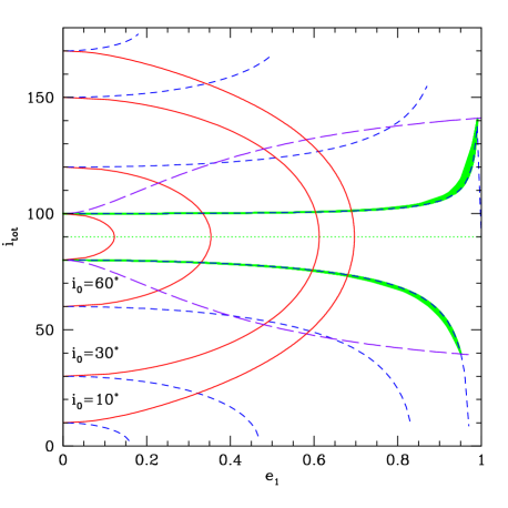
Figure 14: The total inclination and eccentricity relation for an Algol–like system. We show constant energy curves (solid curves, Eq. (66)) and constant total angular momentum curves (dashed curves, Eq. (65)). The initial conditions considered here are $e_{1}^{0}=0$, $g_{1}^{0}$, $e_{2}^{0}=0$ and $L_{1}/L_{2}=0.07$, appropriate for the Algol system (see Section 5.4). We consider four different initial inclinations and their symmetric $90^{\circ}$ counterparts, from bottom to top $10,30,60$ and $80$ degrees. We also show an example (highlighted curve) for the system which is a result of integration of the quadrupole-level approximation equations.

For simplicity we set initially $e_{1}^{0}=0$, $g_{1}^{0}$ and $e_{2}^{0}=0$ (the superscript $0$ stand for initial values). In this appendix we consider only the quadrupole-level approximation, and thus $e_{2}$ doesn’t change. Using these initial conditions (and for some initial mutual inclination $i_{0}$) we can write equation (62) as

$$\sqrt{1-e^{2}_{1}}\cos i_{\mathrm{tot}}=\cos i_{0}+\frac{L_{1}}{2L_{2}}e_{1}^{2}\ .$$ (65)

We show these curves for different $i_{0}$ in Figure 14 (short dashed curves) for a hypothetical system with the parameters of an Algol–like system (but with $e_{2}=0$, see §5.4). Note that there is a slight asymmetry between the prograde and retrograde orbits due to the $L_{1}/L_{2}$ factor (which is not the case for the test particle case, see Lithwick and Naoz, 2011; Katz et al., 2011). Similar analysis for the Algol system was done in Söderhjelm (2006, Figure 1). We also write equations (63) and (64) using the initial conditions. Equation (63) can be simplified to

$$(1-e^{2}_{1})\cos^{2}i_{\mathrm{tot}}=\cos^{2}i_{0}-2e_{1}^{2}\ ,$$ (66)

depicted in Figure 14 (solid curves, for different $i_{0}$). As can be seen from the Figure, this equation gives the minimum eccentricity, which is the crossing point with equation (65). For these choice of initial conditions the minimum eccentricity is $e_{1}^{0}=0$. Equation (64) becomes

$$(1+4e^{2}_{1})\cos^{2}i_{\mathrm{tot}}=\cos^{2}i_{0}+3e_{1}^{2}\ ,$$ (67)

which is depicted in Figure 14 (long dashed curves, for $i_{0}=80^{\circ}$ and $100^{\circ}$). We now use this equation and equation (65) to find the maximum eccentricity. After some algebra we find:

$$\left(\frac{L_{1}}{L_{2}}\right)^{2}e_{1}^{4}+\left(3+4\frac{L_{1}}{L_{2}}\cos i_{0}+\left(\frac{L_{1}}{2L_{2}}\right)^{2}\right)e_{1}^{2}$$

$$+\frac{L_{1}}{L_{2}}\cos i_{0}-3+5\cos^{2}i_{0}=0\ .$$ (68)

As we approach the TPQ limit, $L_{2}\gg L_{1}$, and this equation becomes

$$e^{2}_{1}=1-\frac{5}{3}\cos^{2}i_{0}\ ,$$ (69)

which gives the maximum eccentricity as a function of mutual initial inclination with zero initial inner eccentricity. In Figure 14 we show that this approximation still holds fairly well even for an Algol–like system, where $L_{1}/L_{2}\sim 0.07$. Equation (69) has been found previously (e.g. Innanen et al., 1997; Kinoshita and Nakai, 1999; Valtonen and Karttunen, 2006) in the TPQ approximation, but in these works it is assumed valid outside that limit. A solution exists only if the right hand side of this equations is positive, thus we find the critical angles for large Kozai oscillation in the TPQ limit:

$$39.2^{\circ}\leq i_{0}\leq 140.8^{\circ}\ .$$ (70)

For larger $L_{1}/L_{2}$ and/or for initial $e_{1}>0$ this limit and $e_{\rm max}$ are different and the full solution of equations (62),(63) and (64) is required. In fact for each initial set of $e_{1}>0$ and $i_{\mathrm{tot}}$, there is a specific $L_{1}/L_{2}$ that will produce an angular momentum curve that crosses $90^{\circ}$. Thus, for initial $g_{1}>90^{\circ}$ the mutual inclination can oscillate from value below $90^{\circ}$ to above. This happens because the inclination of the outer orbit $i_{2}$ changes considerably, while the inner orbit retains its prograde or retrograde orientation.

Appendix B The Full Octupole-Order Equations of Motion

We define:

$$C_{3}=-\frac{15}{16}\frac{k^{4}}{4}\frac{(m_{1}+m_{2})^{9}}{(m_{1}+m_{2}+m_{3})^{4}}\frac{m_{3}^{9}(m_{1}-m_{2})}{(m_{1}m_{2})^{5}}\frac{L_{1}^{6}}{L_{2}^{3}G_{2}^{5}}\ .$$ (71)

Note that this definition differs in sign sign from Ford et al. (2000a), and is consistent with Blaes et al. (2002); Ford et al. (2004). For $m_{1}=m_{2}$ this factor is zero. We also define:

$$A=4+3e_{1}^{2}-\frac{5}{2}B\sin i_{\mathrm{tot}}^{2}\ ,$$ (72)

where

$$B=2+5e^{2}_{1}-7e_{1}^{2}\cos(2g_{1})\ ,$$ (73)

and

$$\cos\phi=-\cos g_{1}\cos g_{2}-\cos i_{\mathrm{tot}}\sin g_{1}\sin g_{2}\ .$$ (74)

As mentioned in Section 4 the evolution equations for $e_{2},g_{2},g_{1}$ and $e_{1}$ can be found correctly from a Hamiltonian that has had $h_{1}$ and $h_{2}$ eliminated by the relation $h_{1}-h_{2}=\pi$; the partial derivatives with respect to the other coordinates and momenta are not affected by the substitution. The time evolution of $H_{1}$ and $H_{2}$ (and thus $i_{1}$ and $i_{2}$) can be derived from the total angular momentum conservation. Thus it is useful to write the much simpler the doubly averaged Hamiltonian after eliminating the nodes:

$$\mathcal{H}(\Delta h\to\pi) = C_{2}\{\left(2+3e_{1}^{2}\right)\left(3\cos^{2}i_{\mathrm{tot}}-1\right)$$

$$+ 15e_{1}^{2}\sin^{2}i_{\mathrm{tot}}\cos(2g_{1})\}$$

$$+ C_{3}e_{1}e_{2}\{A\cos\phi$$

$$+ 10\cos i_{\mathrm{tot}}\sin^{2}i_{\mathrm{tot}}(1-e_{1}^{2})\sin g_{1}\sin g2\}\ .$$

The time evolution of the argument of periapse for the inner and outer orbits are given by:

$$\dot{g}_{1} = 6C_{2}\bigg{\{}\frac{1}{G_{1}}[4\cos^{2}i_{\mathrm{tot}}+(5\cos(2g_{1})-1)$$

$$\times (1-e_{1}^{2}-\cos^{2}i_{\mathrm{tot}})]+\frac{\cos i_{\mathrm{tot}}}{G_{2}}[2+e^{2}_{1}(3-5\cos(2g_{1}))]\bigg{\}}$$

$$- C_{3}e_{2}\bigg{\{}e_{1}\left(\frac{1}{G_{2}}+\frac{\cos i_{\mathrm{tot}}}{G_{1}}\right)$$

$$\times [\sin g_{1}\sin g_{2}(10(3\cos^{2}i_{\mathrm{tot}}-1)(1-e_{1}^{2})+A)$$

$$- 5B\cos i_{\mathrm{tot}}\cos\phi]-\frac{1-e_{1}^{2}}{e_{1}G_{1}}\times[\sin g_{1}\sin g_{2}$$

$$\times 10\cos i_{\mathrm{tot}}\sin i_{\mathrm{tot}}^{2}(1-3e_{1}^{2})$$

$$+ \cos\phi(3A-10\cos i_{\mathrm{tot}}^{2}+2)]\bigg{\}}\ ,$$

and

$$\dot{g}_{2} = 3C_{2}\bigg{\{}\frac{2\cos i_{\mathrm{tot}}}{G_{1}}[2+e_{1}^{2}(3-5\cos(2g_{1}))]$$

$$+ \frac{1}{G_{2}}[4+6e_{1}^{2}+(5\cos^{2}i_{\mathrm{tot}}-3)(2+e_{1}^{2}[3-5\cos(2g_{1})])\bigg{\}}$$

$$+ C_{3}e_{1}\bigg{\{}\sin g_{1}\sin g_{2}\bigg{(}\frac{4e_{2}^{2}+1}{e_{2}G_{2}}10\cos i_{\mathrm{tot}}\sin^{2}i_{\mathrm{tot}}(1-e_{1}^{2})$$

$$- e_{2}\left(\frac{1}{G_{1}}+\frac{\cos i_{\mathrm{tot}}}{G_{2}}\right)[A+10(3\cos^{2}i_{\mathrm{tot}}-1)(1-e^{2}_{1})]\bigg{)}$$

$$+ \cos\phi\bigg{[}5B\cos i_{\mathrm{tot}}e_{2}\left(\frac{1}{G_{1}}+\frac{\cos i_{\mathrm{tot}}}{G_{2}}\right)+\frac{4e_{2}^{2}+1}{e_{2}G_{2}}A\bigg{]}\bigg{\}}$$

The time evolution of the longitude of ascending nodes is given by:

$$\dot{h}_{1} = -\frac{3C_{2}}{G_{1}\sin i_{1}}\left(2+3e_{1}^{2}-5e_{1}^{2}\cos\left(2g_{1}\right)\right)\sin\left(2i_{\rm tot}\right)$$

$$- C_{3}e_{1}e_{2}[5B\cos i_{\mathrm{tot}}\cos\phi$$

$$- A\sin g_{1}\sin g_{2}+10(1-3\cos^{2}i_{\mathrm{tot}})$$

$$\times (1-e_{1}^{2})\sin g_{1}\sin g_{2}]\frac{\sin i_{\mathrm{tot}}}{G_{1}\sin i_{1}}\ ,$$

where in the last part we have used again the law of sines for which $\sin i_{1}=G_{2}\sin i_{\mathrm{tot}}/G_{\mathrm{tot}}$. The evolution of the longitude of ascending nodes for the outer orbit can be easily obtained using:

$$\dot{h}_{2}=\dot{h}_{1}\ .$$ (79)

The evolution of the eccentricities is:

$$\dot{e}_{1} = C_{2}\frac{1-e_{1}^{2}}{G_{1}}[30e_{1}\sin^{2}i_{\mathrm{tot}}\sin(2g_{1})]$$

$$+ C_{3}e_{2}\frac{1-e_{1}^{2}}{G_{1}}[35\cos\phi\sin^{2}i_{\mathrm{tot}}e_{1}^{2}\sin(2g_{1})$$

$$- 10\cos i_{\mathrm{tot}}\sin^{2}i_{\mathrm{tot}}\cos g_{1}\sin g_{2}(1-e_{1}^{2})$$

$$- A(\sin g_{1}\cos g_{2}-\cos i_{\mathrm{tot}}\cos g_{1}\sin g_{2})]\ ,$$

and

$$\dot{e}_{2} = -C_{3}e_{1}\frac{1-e_{2}^{2}}{G_{2}}[10\cos\left(i_{\mathrm{tot}}\right)\sin^{2}\left(i_{\mathrm{tot}}\right)(1-e_{1}^{2})\sin g_{1}\cos g_{2}$$ (81)

$$+ A(\cos g_{1}\sin g_{2}-\cos(i_{\mathrm{tot}})\sin g_{1}\cos g_{2})]\ .$$

We also write the angular momenta derivatives as a function of time; for the inner orbit

$$\dot{G}_{1} = -C_{2}30e_{1}^{2}\sin(2g_{1})\sin^{2}(i_{\mathrm{tot}})+C_{3}e_{1}e_{2}($$

$$- 35e_{1}^{2}\sin^{2}(i_{\mathrm{tot}})\sin(2g_{1})\cos\phi+A[\sin g_{1}\cos g_{2}$$

$$- \cos(i_{\mathrm{tot}})\cos g_{1}\sin g_{2}]$$

$$+ 10\cos(i_{\mathrm{tot}})\sin^{2}(i_{\mathrm{tot}})[1-e_{1}^{2}]\cos g_{1}\sin g_{2})\ ,$$

and for the outer orbit (where the quadrupole term is zero)

$$\dot{G}_{2} = C_{3}e_{1}e_{2}[A\{\cos g_{1}\sin g_{2}-\cos(i_{\mathrm{tot}})\sin g_{1}\cos g_{2}\}$$ (83)

$$+ 10\cos(i_{\mathrm{tot}})\sin^{2}(i_{\mathrm{tot}})[1-e_{1}^{2}]\sin g_{1}\cos g_{2}]\ .$$

Also,

$$\dot{H}_{1}=\frac{G_{1}}{G_{\mathrm{tot}}}\dot{G}_{1}-\frac{G_{2}}{G_{\mathrm{tot}}}\dot{G}_{2}\ ,$$ (84)

where using the law of sines we write:

$$\dot{H}_{1}=\frac{\sin i_{2}}{\sin i_{\mathrm{tot}}}\dot{G}_{1}-\frac{\sin i_{1}}{\sin i_{\mathrm{tot}}}\dot{G}_{2}\ .$$ (85)

The inclinations evolve according to

$$\dot{(\cos i_{1})}=\frac{\dot{H}_{1}}{G_{1}}-\frac{\dot{G}_{1}}{G_{1}}\cos i_{1}\ ,$$ (86)

and

$$\dot{(\cos i_{2})}=\frac{\dot{H}_{2}}{G_{2}}-\frac{\dot{G}_{2}}{G_{2}}\cos i_{2}\ .$$ (87)

Our equations are equivalent to those of Ford et al. (2000a), but we give the evolution equations for $H_{1}$ and $H_{2}$ (and $i_{1}$ and $i_{2}$).

Appendix C Elimination of the Nodes and the Problem in Previous Quadrupole-Level Treatments

Since the total angular momentum is conserved, the ascending nodes relative to the invariable plane follow a simple relation, $h_{1}(t)=h_{2}(t)-\pi$. If one inserts this relation into the Hamiltonian, which only depends on $h_{1}-h_{2}$, the resulting “simplified” Hamiltonian is independent of $h_{1}$ and $h_{2}$. One might be tempted to conclude that the conjugate momenta $H_{1}$ and $H_{2}$ are constants of the motion. However, that conclusion is false. This incorrect argument has been made by a number of authors.

In general, using dynamical information about the system—in this case that angular momentum is conserved, implying that ${\bf G}_{1}+{\bf G}_{2}={\bf G}_{\mathrm{tot}}$ at all times and therefore $h_{1}-h_{2}=\pi$—to simplify the Hamiltonian is not correct. The derivation of Hamilton’s equations relies on the possibility of making arbitrary variations of the system’s trajectory, and such simplifications restrict the allowed variations to those which respect the dynamical constraints. Once Hamilton’s equations are employed to derive equations of motion for the system, however, dynamical information can be employed to simplify these equations.

In our particular case, equations of motion for components of the system that do not involve partial derivatives with respect to $h_{1}$ or $h_{2}$ will not be affected by the node-elimination substitution. For this reason, it is correct to derive equations of motion for all components except for $H_{1}$ and $H_{2}$ from the node-eliminated Hamiltonian; expressions for $\dot{H}_{1}$ and $\dot{H}_{2}$ can then be derived from conservation of angular momentum. This approach has been employed in at least one computer code for octupole evolution, though the discussion in the corresponding paper incorrectly eliminates the nodes in the Hamiltonian (Ford et al., 2000a).

In some later studies, (Sidlichovsky, 1983; Innanen et al., 1997; Kiseleva et al., 1998; Eggleton et al., 1998; Mikkola and Tanikawa, 1998; Kinoshita and Nakai, 1999; Eggleton and Kiseleva-Eggleton, 2001; Wu and Murray, 2003; Valtonen and Karttunen, 2006; Fabrycky and Tremaine, 2007; Wu et al., 2007; Zdziarski et al., 2007; Perets and Fabrycky, 2009), the assumption that $H_{1}={\rm const}$ (i.e. the TPQ approximation) was built into the calculations of quadrupole-level secular evolution for various astrophysical systems, even when the condition $G_{2}\gg G_{1}$ was not satisfied. Moreover many previous studies simply set $i_{2}=0$. This is equivalent to the TPQ approximation; for non-test particles, given the mutual inclination $i$, the inner and outer inclinations $i_{1}$ and $i_{2}$ are set by the conservation of total angular momentum [see equations (9) and (10)].

References

- Albrecht et al. (2012) Albrecht, S., Winn, J. N., Johnson, J. A., Howard, A. W., Marcy, G. W., Butler, R. P., Arriagada, P., Crane, J. D., Shectman, S. A., Thompson, I. B., Hirano, T., Bakos, G., and Hartman, J. D. (2012). Obliquities of Hot Jupiter host stars: Evidence for tidal interactions and primordial misalignments. ArXiv e-prints.
- Bailey et al. (1992) Bailey, M. E., Chambers, J. E., and Hahn, G. (1992). Origin of sungrazers - A frequent cometary end-state. Aap, 257, 315–322.
- Baron et al. (2012) Baron, F., Monnier, J. D., Pedretti, E., Zhao, M., Schaefer, G., Parks, R., Che, X., Thureau, N., ten Brummelaar, T. A., McAlister, H. A., Ridgway, S. T., Farrington, C., Sturmann, J., Sturmann, L., and Turner, N. (2012). Imaging the Algol Triple System in H Band with the CHARA Interferometer. ArXiv e-prints.
- Blaes et al. (2002) Blaes, O., Lee, M. H., and Socrates, A. (2002). The Kozai Mechanism and the Evolution of Binary Supermassive Black Holes. ApJ, 578, 775–786.
- Boley et al. (2012) Boley, A. C., Payne, M. J., Corder, S., Dent, W. R. F., Ford, E. B., and Shabram, M. (2012). Constraining the Planetary System of Fomalhaut Using High-resolution ALMA Observations. ApJ Lett, 750, L21.
- Borkovits et al. (2004) Borkovits, T., Forgács-Dajka, E., and Regály, Z. (2004). Tidal and rotational effects in the perturbations of hierarchical triple stellar systems. I. Numerical model and a test application for ¡ASTROBJ¿Algol¡/ASTROBJ¿. Aap, 426, 951–961.
- Brouwer (1959) Brouwer, D. (1959). Solution of the problem of artificial satellite theory without drag. AJ, 64, 378–+.
- Carruba et al. (2002) Carruba, V., Burns, J. A., Nicholson, P. D., and Gladman, B. J. (2002). On the Inclination Distribution of the Jovian Irregular Satellites. Icarus, 158, 434–449.
- Chambers and Migliorini (1997) Chambers, J. E. and Migliorini, F. (1997). Mercury - A New Software Package for Orbital Integrations. In AAS/Division for Planetary Sciences Meeting Abstracts #29, volume 29 of Bulletin of the American Astronomical Society, pages 1024–+.
- Chatterjee et al. (2008) Chatterjee, S., Ford, E. B., Matsumura, S., and Rasio, F. A. (2008). Dynamical Outcomes of Planet-Planet Scattering. ApJ, 686, 580–602.
- Correia et al. (2011) Correia, A. C. M., Laskar, J., Farago, F., and Boué, G. (2011). Tidal evolution of hierarchical and inclined systems. ArXiv e-prints.
- Ćuk and Burns (2004) Ćuk, M. and Burns, J. A. (2004). On the Secular Behavior of Irregular Satellites. AJ, 128, 2518–2541.
- Donnison and Mikulskis (1995) Donnison, J. R. and Mikulskis, D. F. (1995). The effect of eccentricity on three-body orbital stability criteria and its importance for triple star systems. MNRAS, 272, 1–10.
- Eggleton and Kiseleva-Eggleton (2001) Eggleton, P. P. and Kiseleva-Eggleton, L. (2001). Orbital Evolution in Binary and Triple Stars, with an Application to SS Lacertae. ApJ, 562, 1012–1030.
- Eggleton et al. (1998) Eggleton, P. P., Kiseleva, L. G., and Hut, P. (1998). The Equilibrium Tide Model for Tidal Friction. ApJ, 499, 853–+.
- Eggleton et al. (2007) Eggleton, P. P., Kisseleva-Eggleton, L., and Dearborn, X. (2007). The Incidence of Multiplicity Among Bright Stellar Systems. In W. I. Hartkopf, E. F. Guinan, & P. Harmanec, editor, IAU Symposium, volume 240 of IAU Symposium, pages 347–355.