Secular Evolution of Hierarchical Triple Star Systems

Abstract

We derive octupole-level secular perturbation equations for hierarchical triple systems, using classical Hamiltonian perturbation techniques. Our equations describe the secular evolution of the orbital eccentricities and inclinations over timescales long compared to the orbital periods. By extending previous work done to leading (quadrupole) order to octupole level (i.e., including terms of order $\alpha^{3}$, where $\alpha\equiv a_{1}/a_{2}<1$ is the ratio of semimajor axes) we obtain expressions that are applicable to a much wider range of parameters. In particular, our results can be applied to high-inclination as well as coplanar systems, and our expressions are valid for almost all mass ratios for which the system is in a stable hierarchical configuration. In contrast, the standard quadrupole-level theory of Kozai gives a vanishing result in the limit of zero relative inclination. The classical planetary perturbation theory, while valid to all orders in $\alpha$, applies only to orbits of low-mass objects orbiting a common central mass, with low eccentricities and low relative inclination. For triple systems containing a close inner binary, we also discuss the possible interaction between the classical Newtonian perturbations and the general relativistic precession of the inner orbit. In some cases we show that this interaction can lead to resonances and a significant increase in the maximum amplitude of eccentricity perturbations. We establish the validity of our analytic expressions by providing detailed comparisons with the results of direct numerical integrations of the three-body problem obtained for a large number of representative cases. In addition, we show that our expressions reduce correctly to previously published analytic results obtained in various limiting regimes. We also discuss applications of the theory in the context of several observed triple systems of current interest, including the millisecond pulsar PSR B1620$-$26 in M4, the giant planet in 16 Cygni, and the protostellar binary TMR-1.

1 Introduction

About one third of all binary star systems are thought to be members of larger multiple systems. Most of these are hierarchical triples, in which the (inner) binary is orbited by a third body in a much wider orbit (see Tokovinin 1997a,b for recent results and compilations). Secular perturbations in triples result from the gravitational interaction between the inner binary and the outer object, possibly coupled to other processes such as stellar evolution, tidal effects, or, for compact objects, general relativistic effects. In strongly hierarchical triples, the two orbits never approach each other closely, and an analytic, perturbative approach can be used to calculate the evolution of the system. One particularly important perturbation is that of the orbital eccentricities. As the two orbits torque each other and exchange angular momentum, their eccentricities will undergo periodic oscillations over secular timescales (i.e., very long compared to the orbital periods). For non-coplanar systems, corresponding oscillations occur in the orbital inclinations. In contrast, according to canonical perturbation theory, there is no secular change in the semimajor axes, since the energy exchange between the two orbits averages out to zero over long timescales (see, e.g., Heggie 1975).

For triple systems that begin their life near the stability limit, the result of an eccentricity increase can be catastrophic, leading to a collision between the two inner stars, if they started as a close pair, or, more typically, to the disintegration of the triple. This disintegration proceeds through a phase of chaotic evolution whose outcome is the ejection of one of the three stars (typically the least massive body) on an unbound trajectory, while the other two are left in a more tightly bound binary. A striking example of this process was revealed by the recent HST/NICMOS observations of the TMR-1 system in the Taurus star-forming region (Terebey et al. 1998). The HST images reveal a faint companion, most likely a giant planet or brown dwarf, that appears to have been ejected from its parent protostellar binary system. More indirect observational evidence is provided in the form of binary systems with anomalously high space velocities. In particular, the disintegration of short-lived triples formed in dense star forming regions may lead to binary OB runaway stars with very large peculiar velocities, such as HD 3950 (Gies & Bolton 1986).

The stability of triple systems has been the subject of many theoretical studies. Most recently, Eggleton & Kiseleva (1995 and references therein) performed numerical experiments and provided an empirical stability criterion in terms of a critical ratio $Y_{\rm min}$ between the periastron distance of the outer orbit to the apastron distance of the inner orbit. For systems containing three nearly equal masses, one finds $Y_{\rm min}\simeq 3-6$ depending on initial phases, eccentricities and inclinations. Holman & Wiegert (1999) study the stability of planets in binary systems, both for planets orbiting close to one of the two stars, and for planets orbiting outside the binary. All these stability analyses are based on numerical integrations of the three-body problem that are limited to $10^{4}-10^{6}$ periods of the outer orbit. In some cases, however, the secular evolution timescale of the triple can be much longer than this, and therefore systems that remain stable for the duration of the numerical integration may in fact turn out to be unstable over secular timescales. Analytic results such as those derived here can therefore help determining more accurate stability criteria, e.g., by integrating the secular evolution equations and verifying that the stability ratio remains $>Y_{\rm min}$ over the entire cycle of secular perturbations.

Hierarchical triple star systems can play an important role in the dynamical evolution of dense star clusters containing primordial binaries. The cores of globular clusters, for example, are thought to contain a small but dynamically significant population of triple systems formed through dynamical interactions between primordial binaries (McMillan, Hut, & Makino 1991). Both stable and unstable triples can form easily through exchange and resonant interactions between binaries. In direct $N$-body integrations of the cluster dynamics, marginally stable or unstable triples can represent a significant computational bottleneck, since they require very long integrations of the orbital dynamics in order to resolve the outcome of the interaction (see, e.g., Mikkola 1997).

Direct observational evidence for the dynamical production of triple systems in globular clusters is provided by the millisecond pulsar system PSR B1620$-$26 (Rasio, McMillan, & Hut 1995; Ford et al. 2000). This radio pulsar is a member of a hierarchical triple system located in the core of the globular cluster M4. The inner binary of the triple contains the $\simeq 1.4M_{\odot}$ neutron star with a $\simeq 0.3M_{\odot}$ white-dwarf companion in a 191-day orbit (Lyne et al. 1988; McKenna & Lyne 1988). The triple nature of the system was first proposed by Backer (1993) in order to explain the unusually high residual second and third pulse frequency derivatives left over after subtracting a standard Keplerian model for the pulsar binary. The pulsar has now been timed for eleven years since its discovery (see Thorsett et al. 1999 for the most recent update). These observations have not only confirmed the triple nature of the sytem, but they have also provided tight constraints on the mass and orbital parameters of the second companion. Theoretical modeling of the latest timing data (now including five pulse frequency derivatives) and preliminary measurements of the orbital perturbations of the inner binary have further constrained the mass of the second companion, and strongly suggest that it is a giant planet or a brown dwarf of mass $\sim 0.01\,M_{\odot}$ at a distance of $\sim 50\,$AU from the pulsar binary (Joshi & Rasio 1997; Ford et al. 2000).

Our treatment of the secular perturbations in this paper is based on classical celestial mechanics techniques and assumes that all three bodies are unevolving point masses. Whenever the stellar evolution time of one of the components becomes comparable to any of the orbital perturbation timescales computed here, the evolution of the triple can be affected significantly through mass losses, or mass transfer. For a recent discussion of stellar evolution in triples, see Iben & Tutukov (1999), who study the production of Type Ia supernovae from the mergers of heavy white dwarfs inside hierarchical triples. Mikkola & Tanikawa (1998) have studied the episodic mass transfer triggered by large eccentricity oscillations of the inner binary in the secular evolution of the triple system CH Cygni. Eggleton & Verbunt (1989) have discussed the possible relevance of triple star evolution for the formation of low-mass X-ray binaries.

Our work focuses on triple systems containing well-separated components, in which the orbital perturbation timescales are short compared to any tidal dissipation time. For triple systems containing a close inner binary, tidal dissipation in the inner components provides a sink of energy and angular momentum which can change substantially the character of the secular perturbations. For a recent discussion of tidal dissipation in triple systems containing a close inner binary, see the paper by Kiseleva, Eggleton, & Mikkola (1998). Bailyn & Grindlay (1987) have discussed the combined effects of tidal interaction and mass transfer for compact X-ray binaries in hierarchical triples. Mazeh & Shaham (1979) were the first to point out that the combination of tidal dissipation and secular eccentricity perturbations in triples could sometimes lead to a substantial orbital shrinking of the inner binary.

One possible additional perturbation effect that we do take into account in this work is the general relativistic precession of the inner orbit if the inner binary contains compact objects. An example is provided by the PSR B1620$-$26 triple system, in which the inner binary contains a neutron star and a white dwarf. When the precession periods from general relativity and from Newtonian perturbations in the triple become comparable, a type of resonant effect is possible which leads to increased magnitudes for the orbital perturbations. A similar resonant effect has been mentioned by Söderhjelm (1984) for triples where the inner binary precesses under the influence of a rotationally-induced quadrupole moment in one of the stars.

Our paper is organized as follows. In §2 we present a derivation of the octupole-order secular perturbation equations and we compare our results to those obtained in the quadrupole approximation and in classical planetary perturbation theory. In §3 the analytic results are compared to direct numerical integrations, and the effects of varying all relevant parameters are explored. In §4 we discuss the effects of the general relativistic precession of the inner orbit on the secular evolution of the triple, using the PSR B1620$-$26 system as an example. In §5 possible applications of our results to other observed triple systems are briefly discussed.

2 Analytic Secular Perturbation Theory

In this section we present a simple analytic treatment of the long-term, secular evolution of hierarchical triple systems using time-independent Hamiltonian perturbation theory in which the small parameter is the ratio of semimajor axes. We discuss essential aspects of the lowest-order (quadrupole-level) approximation, which has been widely used to study hierarchical stellar triples. Then we extend the approximation to the octupole level and compare our results with results from the quadrupole and other approximations to show that the octupole-level equations derived here are valid for a far greater range of parameters.

2.1 Summary of Previous Work

Our derivation of the octupole-level secular perturbation equations is based on classical perturbation methods of celestial mechanics. Studies of the long-term behavior of the solar system led Lagrange and Laplace to the creation of the first classical perturbation theory. Their approach is applicable to a small class of planetary configurations with parameters similar to those of the solar system. The lunar problem was successfully attacked in the end of the last century by Delaunay who was the first to apply the method of canonical transformations to long-term perturbations. This method possesses much greater generality and was used to study a broad spectrum of problems. Brown (1936) was the first to apply canonical averaging to stellar triples, and he obtained the transformed quadrupole Hamiltonian. Kozai (1962) made use of the quadrupole approximation while studying the long-term motion of asteroids and noted several important properties of this approximation. Harrington (1968) obtained quadrupole-level expressions similar to Kozai’s for general hierarchical systems of three stars. Söderhjelm (1984) derived octupole-level equations in the limit of low eccentricities and inclinations. In particular, he demonstrated that the quadrupole approximation fails in this regime because the octupole term in the Hamiltonian becomes dominant. Finally, Marchal (1990) averaged the octupole Hamiltonian keeping all terms up to third order in $\alpha$ and some terms of order $\alpha^{7/2}$. His Hamiltonian truncated at third order is identical to the one used in this paper.

In the process of completing this work, we became aware of related ongoing work by other groups. In particular, Krymolowski & Mazeh (1999) have derived octupole-order perturbation equations following the same method used here. They retain some additional terms, of order $\alpha^{7/2}$, which were also partly included in Marchal’s (1990) Hamiltonian. Based on a few numerical integrations that Krymolowski & Mazeh (1999) provide for a fairly strongly coupled system ($\alpha=0.1$), it appears that these higher-order terms have a negligible effect on the perturbations, although they can lead to slightly shorter periods of eccentricity oscillations for systems with low relative inclination. Eggleton (2000) has used a perturbation method based on the variation of the Runge-Lenz vector (see Heggie & Rasio 1996) to derive an extension of Kozai’s theory to octupole order. Similar work has been done by Georgakarakos (2000), who concentrates on systems where the inner orbit is nearly circular.

2.2 Octupole Theory

A hierarchical triple system consists of a close binary ($m_{0}$ and $m_{1}$) and a third body ($m_{2}$) moving around the inner binary on a much wider orbit. To describe this structure it is convenient to use Jacobi coordinates, which are defined as follows. The vector ${\bf r}_{1}$ represents the position of $m_{1}$ relative to $m_{0}$, and ${\bf r}_{2}$ is the position of $m_{2}$ relative to the center of mass of the inner binary (See Fig. 1). This coordinate system naturally divides the motion of the triple into two separate motions, and makes it possible to write the Hamiltonian as a sum of two terms representing the two decoupled motions and an infinite series representing the coupling of the orbits. Let the subscripts 1 and 2 refer to the inner and outer orbits, respectively. The coupling term is written as a power series in the ratio of the semi-major axes $\alpha\equiv{a_{1}}/{a_{2}}$, which serves as the small parameter in our perturbation expansion. The complete Hamiltonian of the three-body system is given by (Harrington 1968)

$${\cal F}=\frac{k^{2}m_{0}m_{1}}{2a_{1}}+\frac{k^{2}(m_{0}+m_{1})m_{2}}{2a_{2}}+\frac{k^{2}}{a_{2}}\,\sum_{j=2}^{\infty}\alpha^{j}M_{j}\left(\frac{r_{1}}{a_{1}}\right)^{j}\left(\frac{a_{2}}{r_{2}}\right)^{j+1}P_{j}(\cos\Phi),$$ (1)

where $k^{2}$ is the gravitational constant, $P_{j}$’s are the Legendre polynomials, $\Phi$ is the angle between ${\bf r}_{1}$ and ${\bf r}_{2}$, and

$$M_{j}=m_{0}m_{1}m_{2}\frac{m_{0}^{j-1}-(-m_{1})^{j-1}}{(m_{0}+m_{1})^{j}}.$$ (2)

We shall deal with the expansion only up to third order in $\alpha$.

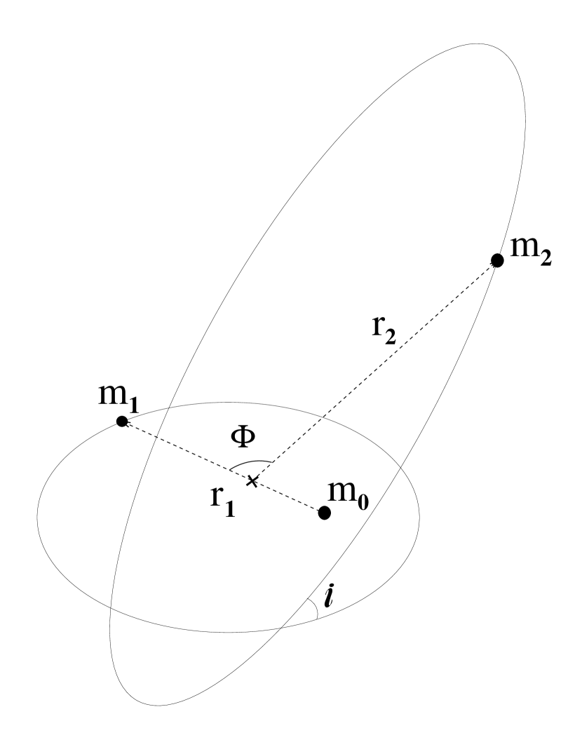
Figure 1: Diagram illustrating the coordinate system used to describe the hierarchical triple system.

Let us define a set of canonical variables, known as Delaunay’s elements, that provide a particularly convenient dynamical description of our three-body system. The angle variables are chosen to be

$$l_{1},l_{2} = \rm{mean\ anomalies}$$ (3)

$$g_{1},g_{2} = \rm{arguments\ of\ periastron}$$ (4)

$$h_{1},h_{2} = \rm{longitudes\ of\ ascending\ nodes}$$ (5)

and their conjugate momenta

$$L_{1}=\frac{m_{0}m_{1}}{m_{0}+m_{1}}\sqrt{k^{2}(m_{0}+m_{1})a_{1}}\qquad L_{2}=\frac{m_{2}(m_{0}+m_{1})}{m_{0}+m_{1}+m_{2}}\sqrt{k^{2}(m_{0}+m_{1}+m_{2})a_{2}},$$ (6)

$$G_{1}=L_{1}\sqrt{1-e_{1}^{2}}\qquad G_{2}=L_{2}\sqrt{1-e_{2}^{2}},$$ (7)

$$H_{1}=G_{1}\cos i_{1}\qquad H_{2}=G_{2}\cos i_{2},$$ (8)

where $e_{1}$, $e_{2}$ are the orbital eccentricities and $i_{1}$, $i_{2}$ are the orbital inclinations.

The usual canonical relations represent the equations of motion:

$$\frac{dL_{j}}{dt}=\frac{\partial{\cal F}}{\partial l_{j}}\qquad\frac{dl_{j}}{dt}=-\frac{\partial{\cal F}}{\partial L_{j}},$$ (9)

$$\frac{dG_{j}}{dt}=\frac{\partial{\cal F}}{\partial g_{j}}\qquad\frac{dg_{j}}{dt}=-\frac{\partial{\cal F}}{\partial G_{j}},$$ (10)

$$\frac{dH_{j}}{dt}=\frac{\partial{\cal F}}{\partial h_{j}}\qquad\frac{dh_{j}}{dt}=-\frac{\partial{\cal F}}{\partial H_{j}},$$ (11)

where $j=1,2$. Note that $H_{2}$ is the $z$-component of the angular momentum contributed by the perturbing body, the $z$-axis being the direction of the total angular momentum, perpendicular to the invariable plane of the system (See Fig. 2). Equations (9)–(11) appear to have six degrees of freedom, but they can be reduced to four by the theorem of elimination of nodes (Jeffrys & Moser 1966). The Hamiltonian contains $h_{1}$ and $h_{2}$ only in the combination $h_{1}-h_{2}$, and it is symmetric with respect to the orientation of the line of nodes when the invariable plane is chosen as a reference plane. In other words, the Hamiltonian is symmetric with respect to rotations about the total angular momentum vector $\bf H$. Thus, $H_{1}$ and $H_{2}$ enter the Hamiltonian only as $H_{1}+H_{2}=H$ and can be eliminated from the Hamiltonian using the relations

$$H_{1}=\frac{H^{2}+G_{1}^{2}-G_{2}^{2}}{2H}$$ (12)

$$H_{2}=\frac{H^{2}+G_{2}^{2}-G_{1}^{2}}{2H}$$ (13)

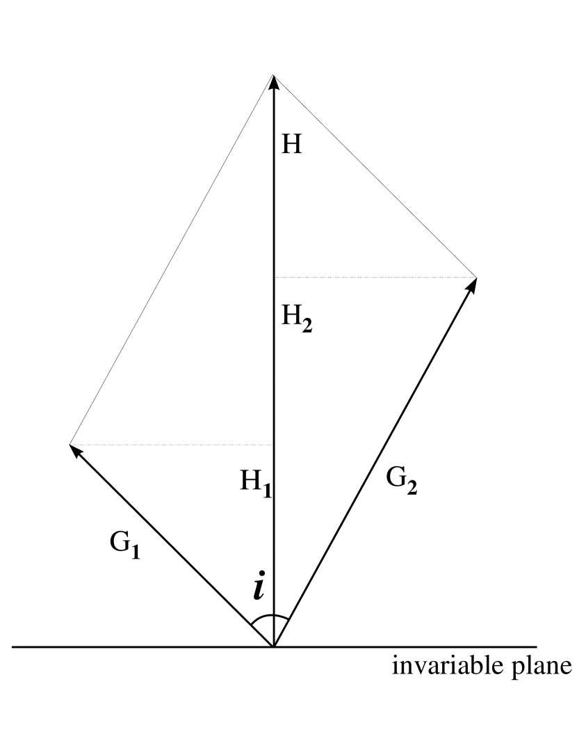
Figure 2: Diagram illustrating the relationships between the canonical variables and angular momenta.

Using the new canonical elements we can write the first four terms of the Hamiltonian (1) as

$${\cal F}_{oct} = {\cal F}_{0}+{\cal F}_{1}+{\cal F}_{2}+{\cal F}_{3}$$ (14)

$$= \frac{\beta_{0}}{2L_{1}^{2}}+\frac{\beta_{1}}{2L_{2}^{2}}+8\beta_{2}\left(\frac{L_{1}^{4}}{L_{2}^{6}}\right)\left(\frac{r_{1}}{a_{1}}\right)^{2}\left(\frac{a_{2}}{r_{2}}\right)^{3}(3\cos^{2}\Phi-1)$$

$$+2\beta_{3}\left(\frac{L_{1}^{6}}{L_{2}^{8}}\right)\left(\frac{r_{1}}{a_{1}}\right)^{3}\left(\frac{a_{2}}{r_{2}}\right)^{4}(5\cos^{3}\Phi-3\cos\Phi),$$

where the mass parameters are

$$\beta_{0} = k^{4}\frac{(m_{0}m_{1})^{3}}{m_{0}+m_{1}},$$ (16)

$$\beta_{1} = k^{4}\frac{(m_{0}+m_{1})^{3}m_{2}^{3}}{m_{0}+m_{1}+m_{2}},$$ (17)

$$\beta_{2} = \frac{k^{4}}{16}\frac{(m_{0}+m_{1})^{7}}{(m_{0}+m_{1}+m_{2})^{3}}\frac{m_{2}^{7}}{(m_{0}m_{1})^{3}},$$ (18)

$$\beta_{3} = \frac{k^{4}}{4}\frac{(m_{0}+m_{1})^{9}}{(m_{0}+m_{1}+m_{2})^{4}}\frac{m_{2}^{9}(m_{0}-m_{1})}{(m_{0}m_{1})^{5}}.$$ (19)

Each term in the series is labeled according to the degree of the Legendre polynomial associated with it (same as the power of $r_{1}/r_{2}$). Following the standard nomenclature associated with multipole expansions we shall call the Hamiltonian containing the first three terms (up to $j=2$) “quadrupole” and the third-order Hamiltonian (2.2) “octupole.” The first two terms in expression (2.2) describe the unperturbed motion of the inner and outer binaries, and the higher-order terms describe the coupling. The quadrupole Hamiltonian contains the perturbation of order $\alpha^{2}$, the octupole Hamiltonian extends this to order $\alpha^{3}$.

The complete Hamiltonian (1) contains the full description of the system. However, we are going to restrict our study to the long-term, secular behavior of the system, by averaging over short-period effects. Even though equation (2.2) is already an approximation of the full Hamiltonian, it contains information about short-period perturbations that needs to be eliminated. In particular the angle $\Phi$ depends on the mean anomalies. Further simplification is achieved through a canonical transformation of variables, called the von Zeipel transformation. Its essence is to replace the Delaunay elements with a set of new canonical coordinates and momenta that rid the Hamiltonian of the dependence on $l_{1}$ and $l_{2}$. The perturbed action variables are still periodic functions of the perturbed angle variables, but the former are no longer linear functions of time. The goal is to find such a set of action-angle variables that the perturbed Hamiltonian will be a function only of the action variables. In the end we can think of the Hamiltonian as describing the interaction between two weighted elliptical rings instead of point masses in orbits.

It is important to note that we do not simply average the Hamiltonian with respect to these variables, since this would destroy the canonical structure of the equations of motion, but instead proceed in a more cautious and intricate manner. We start by requiring that the new Hamiltonian be equal to the old one, since changing variables does not change the energy, and expanding both sides of the equality as Taylor series in $\alpha$. Then we go order by order to identify the terms in the transformed Hamiltonian, using the result of the previous order calculation in each step. The theory behind the Von Zeipel method is very well presented and illustrated by Goldstein (1980, section 11-5) and Hagihara (1972). Additionally, Harrington (1968, 1969) has applied this method to the quadrupole Hamiltonian. We followed exactly the same prescription but all the way to third order. Here we present only the results of the von Zeipel averaging procedure, omitting the laborious algebraic details.

Let us define the following convenient quantities

$$\theta=\cos i=\frac{H^{2}-G_{1}^{2}-G_{2}^{2}}{2G_{1}G_{2}},$$ (20)

where $\bf H=\bf G_{1}+\bf G_{2}$ and $H=|\bf H|$ is given by initial conditions and $i=i_{1}-i_{2}$ is the mutual inclination. The angle $\varphi$ between the directions of periastron is given by

$$\cos\varphi=-\cos g_{1}\cos g_{2}-\theta\sin g_{1}\sin g_{2}.$$ (21)

The doubly-averaged Hamiltonian is given by

$$\bar{\cal F}_{oct} = C_{2}\cdot\{(2+3e_{1}^{2})(3\theta^{2}-1)+15e_{1}^{2}(1-\theta^{2})\cos 2g_{1}\}$$ (22)

$$+C_{3}\cdot e_{1}e_{2}\Big{\{}A\cos\varphi+10\theta(1-\theta^{2})(1-e_{1}^{2})\sin g_{1}\sin g_{2}\Big{\}},$$

where

$$C_{2}=\frac{k^{4}}{16}\frac{(m_{0}+m_{1})^{7}}{(m_{0}+m_{1}+m_{2})^{3}}\frac{m_{2}^{7}}{(m_{0}m_{1})^{3}}\frac{L_{1}^{4}}{L_{2}^{3}G_{2}^{3}},$$ (23)

$$C_{3}=\frac{15}{16}\frac{k^{4}}{4}\frac{(m_{0}+m_{1})^{9}}{(m_{0}+m_{1}+m_{2})^{4}}\frac{m_{2}^{9}(m_{0}-m_{1})}{(m_{0}m_{1})^{5}}\frac{L_{1}^{6}}{L_{2}^{3}G_{2}^{5}},$$ (24)

$$B=2+5e_{1}^{2}-7e_{1}^{2}\cos 2g_{1},$$ (25)

$$A=4+3e_{1}^{2}-\frac{5}{2}(1-\theta^{2})B.$$ (26)

Note that the Hamiltonian (22) does not contain any dependence on $l_{1}$ or $l_{2}$ because these variables have been integrated out as a result of the canonical transformation. The actual differences between the original and the transformed variables are small (of order $\alpha$ or smaller) and periodic. Variables appearing in equation (22) are only approximations of the old variables defined in equations (5)–(8), and they can be thought of as the averages of the old variables. This Hamiltonian is equivalent to the Hamiltonian given by Marchal (1990; see his eqs. [252]–[255]).

The absence of $l_{1}$ and $l_{2}$ from the transformed Hamiltonian implies that $L_{1}$ and $L_{2}$ are constants of the motion, which in turns implies that, in our approximation, the transformed semi-major axes $a_{1}$ and $a_{2}$ are constant. Thus, the only secularly changing parameters in this model are $e_{1}$, $e_{2}$, $g_{1}$, $g_{2}$, and $i$, which is coupled to $e_{1}$ and $e_{2}$ by relation (20). The equations of motion are derived from the Hamiltonian (22) using the canonical relations

$$\frac{de_{i}}{dt}=\frac{\partial e_{i}}{\partial G_{i}}\frac{\partial\bar{\cal F}_{oct}}{\partial g_{i}},$$ (27)

and

$$\frac{dg_{i}}{dt}=-\frac{\partial\bar{\cal F}_{oct}}{\partial G_{i}}.$$ (28)

After regrouping terms, the octupole-level secular perturbation equations follow:

$$\frac{dg_{1}}{dt} = C_{2}\cdot 6\left\{\frac{1}{G_{1}}\left[4\theta^{2}+(5\cos 2g_{1}-1)(1-e_{1}^{2}-\theta^{2})\right]+\frac{\theta}{G_{2}}\left[2+e_{1}^{2}(3-5\cos 2g_{1})\right]\right\}$$ (29)

$$-C_{3}\cdot e_{2}\Bigg{\{}e_{1}\left(\frac{1}{G_{2}}+\frac{\theta}{G_{1}}\right)\Big{[}\sin g_{1}\sin g_{2}\left\{A+10(3\theta^{2}-1)(1-e_{1}^{2})\right\}-5\theta B\cos\varphi\Big{]}$$

$$-\frac{1-e_{1}^{2}}{e_{1}G_{1}}\Big{[}\sin g_{1}\sin g_{2}\cdot 10\theta(1-\theta^{2})(1-3e_{1}^{2})+\cos\varphi(3A-10\theta^{2}+2)\Big{]}\Bigg{\}},$$

$$\frac{de_{1}}{dt} = C_{2}\cdot\frac{1-e_{1}^{2}}{G_{1}}\Big{\{}30e_{1}(1-\theta^{2})\sin 2g_{1}\Big{\}}+C_{3}\cdot e_{2}\frac{1-e_{1}^{2}}{G_{1}}\Big{\{}35\cos\varphi(1-\theta^{2})e_{1}^{2}\sin 2g_{1}$$ (30)

$$-10\theta(1-e_{1}^{2})(1-\theta^{2})\cos g_{1}\sin g_{2}-A(\sin g_{1}\cos g_{2}-\theta\cos g_{1}\sin g_{2})\Big{\}},$$

$$\frac{dg_{2}}{dt} = C_{2}\cdot 3\left\{\frac{2\theta}{G_{1}}\left[2+e_{1}^{2}(3-5\cos 2g_{1})\right]+\frac{1}{G_{2}}\left[4+6e_{1}^{2}+(5\theta^{2}-3)(2+e_{1}^{2}(3-5\cos 2g_{1}))\right]\right\}$$ (31)

$$+C_{3}\cdot e_{1}\Bigg{\{}\sin g_{1}\sin g_{2}\left[\frac{4e_{2}^{2}+1}{e_{2}G_{2}}10\theta(1-\theta^{2})(1-e_{1}^{2})-e_{2}\left(\frac{1}{G_{1}}+\frac{\theta}{G_{2}}\right)(A+10(3\theta^{2}-1)(1-e_{1}^{2}))\right]$$

$$+\cos\varphi\left[5B\theta e_{2}\left(\frac{1}{G_{1}}+\frac{\theta}{G_{2}}\right)+\frac{4e_{2}^{2}+1}{e_{2}G_{2}}A\right]\Bigg{\}},$$

$$\frac{de_{2}}{dt} = -C_{3}\cdot e_{1}\frac{1-e_{2}^{2}}{G_{2}}\Big{\{}10\theta(1-\theta^{2})(1-e_{1}^{2})\sin g_{1}\cos g_{2}+A(\cos g_{1}\sin g_{2}-\theta\sin g_{1}\cos g_{2})\Big{\}}.$$ (32)

This system of coupled nonlinear differential equations describes the octupole-level behavior of hierarchical triples and can be easily integrated numerically to determine the secular evolution of a hierarchical triple for any initial configuration. We found that for calculations with small eccentricities it is better to use the transformed set of variables $e_{1}\sin g_{1}$, $e_{1}\cos g_{1}$, $e_{2}\sin g_{2}$, and $e_{2}\cos g_{2}$. These equations can be integrated numerically much more rapidly than the full equations of motion.

2.3 Comparison with Quadrupole-Level Results

The quadrupole results of Kozai (1962) and Harrington (1969) have found numerous applications in recent studies of planetary, pulsar, and stellar systems. Mazeh & Shaham (1979) calculated the quadrupole-level, long-term periodic behavior of triples and used their results to study high-amplitude eccentricity modulations of systems with large initial inclination. Holman et al. (1997) used the quadrupole-level theory of Kozai to analyze the dynamical evolution of the planet in the binary star 16 Cygni. Rasio, Ford, & Kozinsky (1997) used the same theory to study long-term eccentricity perturbations in the PSR B1620$-$26 pulsar system.

The quadrupole Hamiltonian can be obtained from expression (22) by dropping the $C_{3}$ term:

$${\cal F}_{q}=C_{2}\cdot\{(2+3e_{1}^{2})(3\theta^{2}-1)+15e_{1}^{2}(1-\theta^{2})\cos 2g_{1}\}.$$ (33)

Note that ${\cal F}_{q}$ is independent of $g_{2}$, meaning that, in the quadrupole approximation, $G_{2}$ is a constant of the motion, and so is $e_{2}$ by equation (27). Therefore, to quadrupole order in secular perturbation theory, there is no variation in the eccentricity of the outer orbit. This is a well-known result (see, e.g., Marchal 1990, Sec. 10.2.3). Now there is only one degree of freedom left, so the evolution of the inner eccentricity is described by

$$\frac{dg_{1}}{dt} = C_{2}\cdot 6\left\{\frac{1}{G_{1}}\left[4\theta^{2}+(5\cos 2g_{1}-1)(1-e_{1}^{2}-\theta^{2})\right]+\frac{\theta}{G_{2}}\left[2+e_{1}^{2}(3-5\cos 2g_{1})\right]\right\},$$ (34)

with

$$\frac{de_{1}}{dt} = C_{2}\cdot\frac{1-e_{1}^{2}}{G_{1}}\Big{\{}30e_{1}(1-\theta^{2})\sin 2g_{1}\Big{\}}.$$ (35)

The advantage of using the quadrupole approximation is that it can describe the secular behavior of systems with high relative inclination and a wide range of initial eccentricities, regimes not covered by the classical planetary perturbation theory. As in the classical theory, the quadrupole-level perturbation equations (34)–(35) can be solved exactly for the period and amplitude of oscillation (Kozai 1962). The period of eccentricity oscillations is given approximately by

$$P_{e}\simeq P_{1}\left(\frac{m_{0}+m_{1}}{m_{2}}\right)\left(\frac{a_{2}}{a_{1}}\right)^{3}\left(1-e_{2}^{2}\right)^{3/2},$$ (36)

where $P_{1}$ is the orbital period of the inner binary (Mazeh & Shaham 1978). This expression should be multiplied by a coefficient of order unity which can be obtained using Weierstrass’s zeta function as shown by Kozai (1962).

The secular evolution can be visualized with the help of phase-space diagrams of $e_{1}$ vs $\cos g_{1}$. An example is provided in Figure 3. Each contour corresponds to an initial condition with a certain value of the total angular momentum $H$. Since $G_{2}$ is fixed, $e_{1}$ is coupled to $i$ through equation (20), so the relative inclination oscillates with the same period as $e_{1}$. The up-down symmetry forces similar behavior in $g_{1}$-$e_{1}$ phase space for both $g_{1}\in[-\pi,0]$ and $g_{1}\in[0,\pi]$. One obvious feature is the existence of two regimes: libration and circulation. The libration island generally appears when the initial inclination is greater than some critical value, which for most systems is around $i_{\rm crit}\simeq 40^{\circ}$. Kozai (1962) calculated that for $\alpha\leq 0.10$, $\,38.960^{\circ}\leq i_{\rm crit}\leq 39.231^{\circ}$. From the shape of the large libration island we see that $e_{1}$ can grow from a very small initial value to a very large maximum. Holman et al. (1997) approximate the maximum inner eccentricity as

$$e_{1,{\rm max}}\simeq\left(1-(5/3)\cos^{2}i_{o}\right)^{1/2},$$ (37)

where $i_{o}$ is the initial relative inclination. Libration can occur for low inclinations as well, but this does not lead to large eccentricity oscillations.

Several erroneous features of the quadrupole approximation are worth noting. For an initial condition with $e_{1}=0$, no evolution occurs at all. This is especially significant in a case where there is no libration island, since in that case the eccentricity perturbation would appear to approach zero continuously as the initial eccentricity is decreased. Similarly, in the coplanar case ($\theta=1$), the theory predicts no evolution of eccentricity. From the classical planetary perturbation theory (§2.4), which assumes low eccentricities and inclinations, we know that this is not correct. These features also contradict the octupole-level results (§2.2), as well as the results of direct numerical integrations (§3.2). We conclude that the quadrupole approximation fails for low inclination and for low inner eccentricity. However, it remains qualitatively applicable in the high-inclination regime.

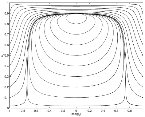
Figure 3: Phase space trajectories obtained in the quadrupole approximation for a system with $m_{2}/m_{1}=10^{-3}$, $m_{3}/m_{1}=1$, $\alpha^{-1}=100$, $e_{2}=0.9$, and initial values of $e_{1}$ ranging from $0.02$ to $0.9$. The libration contours were obtained by setting the initial value of $g_{1}=90^{\circ}$.

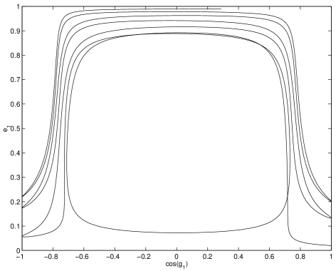
Figure 4: Phase-space trajectory of the same system as in Figure 3 with initial $e_{1}=0.02$, but with the octupole terms included in the integration. (Note that this corresponds to a single trajectory in Fig. 3.)

The octupole-level theory has more degrees of freedom and covers most regimes of hierarchical triple configurations. The perturbation equations (29)–(32) indicate that there are no additional conserved quantities apart from the obvious ones (total angular momentum and total energy). In contrast to the quadrupole theory, the quantities $e_{2}$ and $g_{2}$ now vary with time and the behavior is much harder to visualize. We can notice striking qualitative differences between the two theories by looking at phase-space diagrams. An example is provided in Figure 4. Trajectories are no longer closed, and transitions between libration and circulation occur, since the angular momentum of the outer orbit now evolves with time. Thus, we now have more than one frequency in the secular oscillations.

Figure 5 demonstrates that a system can have a qualitatively different behavior from what is expected in the quadrupole approximation. While the quadrupole theory predicts periodic variations of constant amplitude, according to the octupole equations (and in agreement with the results of a direct numerical integration) the amplitude grows very close to unity. This leads to a very small periastron distance and the possibility of a tidal interaction or collision between the two inner stars. Thus, one must exercise great caution when modeling systems using the quadrupole approximation. Ignoring octupole-level terms can lead to completely invalid results.

Figure 5: These results illustrate the potential danger of using the quadrupole approximation. The inner eccentricity is shown as a function of time for a system with $m_{1}/m_{0}=10^{-3}$, $m_{2}/m_{1}=1$, $\alpha^{-1}=100$, initial eccentricities $e_{1}=0.05$ and $e_{2}=0.9$, and an initial relative inclination $i=70^{\circ}$. Time is given in years assuming $a_{1}=1\,$AU and $m_{0}=1\,M_{\odot}$. The solid line is from the integration of the octupole-level perturbation equations, while the dashed line is from a direct numerical integration of the three-body system (see §3.1). In the quadrupole approximation all oscillations would have the same amplitude as the first shown here. Notice how the eccentricity oscillations in fact increase in amplitude, making the inner periastron separation quite small. At some point other effects such as general relativistic precession and tidal dissipation (not to mention a collision between the two inner stars) could become significant.

2.4 Comparison with Classical Planetary Perturbation Theory

For application to many problems in the context of the Solar System, a classical perturbation theory was developed many years ago that applies to low-eccentricity, low-inclination orbits of planets around a central star (one dominant mass). This theory does not assume that the ratio of semimajor axes is small, and therefore it provides results valid to all orders in $\alpha$. A detailed account of the planetary theory can be found in Brouwer & Clemence (1961, Chap. 16). For an excellent pedagogic summary, see Dermott & Nicholson (1986). Rasio (1994, 1995) used the classical theory to study the eccentricity perturbations in the PSR B1620-26 triple system in the limit of coplanar orbits, and derived simple approximate expressions for the period and amplitude of eccentricity oscillations in various limits.

Here we will only consider the variations of the eccentricities, since the results for inclinations are very similar. It turns out that the inclination evolution is decoupled from the eccentricity evolution, and so the two can be solved separately. Because eccentricities are very small and can vanish, it is better to use the variables

$$h_{1}=e_{1}\sin g_{1}\qquad h_{2}=e_{2}\sin g_{2}$$ (38)

$$k_{1}=e_{1}\cos g_{1}\qquad k_{2}=e_{2}\cos g_{2}.$$ (39)

Since angular momentum is conserved and the mutual inclination stays constant to first order, the two eccentricities vary $90^{\circ}$ out of phase. The linear system of equations describing the secular evolution of eccentricities in planetary perturbation theory is

$$\frac{dh_{1}}{dt}=+A_{11}k_{1}-A_{12}k_{2}$$ (40)

$$\frac{dk_{1}}{dt}=-A_{11}h_{1}+A_{12}h_{2}$$ (41)

$$\frac{dh_{2}}{dt}=-A_{21}k_{1}+A_{22}k_{2}$$ (42)

$$\frac{dk_{2}}{dt}=+A_{21}h_{1}-A_{22}h_{2},$$ (43)

where the $A$’s are defined in terms of Laplace coefficients, which we truncate at third order in $\alpha$ to obtain

$$A_{11}=\frac{3}{4}k\frac{\tilde{a}_{1}^{3/2}}{\tilde{a}_{2}^{3}}\frac{m_{2}}{\sqrt{m_{0}+m_{1}}},\qquad A_{12}=\frac{15}{16}k\frac{\tilde{a}_{1}^{5/2}}{\tilde{a}_{2}^{4}}\frac{m_{2}}{\sqrt{m_{0}+m_{1}}},$$ (44)

$$A_{21}=\frac{15}{16}k\frac{\tilde{a}_{1}^{3}}{\tilde{a}_{2}^{9/2}}\frac{m_{1}}{\sqrt{m_{0}+m_{2}}},\qquad A_{22}=\frac{3}{4}k\frac{\tilde{a}_{1}^{2}}{\tilde{a}_{2}^{7/2}}\frac{m_{1}}{\sqrt{m_{0}+m_{2}}},$$ (45)

where $\tilde{a}_{1}$ and $\tilde{a}_{2}$ are the averaged semimajor axes measured from $m_{0}$ to $m_{1}$ and $m_{2}$, respectively.

Now we rewrite the system in terms of familiar quantities to find

$$\frac{de_{1}}{dt}=A_{12}e_{2}\sin g,$$ (46)

$$\frac{de_{2}}{dt}=-A_{21}e_{1}\sin g,$$ (47)

$$\frac{dg}{dt}=A_{22}-A_{11}+A_{12}\frac{e_{2}}{e_{1}}\cos g-A_{21}\frac{e_{1}}{e_{2}}\cos g,$$ (48)

where $g=g_{2}-g_{1}$. Indeed the use of this variable is convenient, since for coplanar orbits there is no well-defined line of nodes, and only the relative longitudes of perihelia are important.

Upon expanding the octupole equations (29)–(32) to first order in $e_{1}$ and $e_{2}$ we obtain an identical linear system of differential equations, but with the $A$’s replaced by

$$B_{11} = \frac{12C_{2}}{L_{1}}=\frac{3}{4}k\frac{a_{1}^{3/2}}{a_{2}^{3}}\frac{m_{2}}{\sqrt{m_{0}+m_{1}}},$$ (49)

$$B_{12} = \frac{4C_{3}}{L1}\ =\frac{15}{16}k\frac{a_{1}^{5/2}}{a_{2}^{4}}\frac{m_{2}(m_{0}-m_{1})}{(m_{0}+m_{1})^{3/2}},$$ (50)

$$B_{21} = \frac{4C_{3}}{L_{2}}=\frac{15}{16}k\frac{a_{1}^{3}}{a_{2}^{9/2}}\frac{m_{0}m_{1}(m_{0}-m_{1})\sqrt{m_{0}+m_{1}+m_{2}}}{(m_{0}+m_{2})^{3}},$$ (51)

$$B_{22} = \frac{12C_{2}}{L_{2}}=\frac{3}{4}k\frac{a_{1}^{2}}{a_{2}^{7/2}}\frac{m_{0}m_{1}\sqrt{m_{0}+m_{1}+m_{2}}}{(m_{0}+m_{1})^{2}}.$$ (52)

It is easy to see that, in the limit where $m_{0}\gg m_{1}$ and $m_{0}\gg m_{2}$, the two sets of equations coincide, as they should. This establishes the accuracy of our analytic results in this limit.

In general, the two sets of equations differ in the dependence of the coefficients on the masses. Although the two theories use different coordinate systems (Jacobi vs heliocentric), this alone does not explain the difference. Instead, one must remember that the classical theory was derived from Lagrange’s planetary equations (see Brouwer & Clemence 1961), which assume that the disturbing functions (proportional to $m_{1}$ and $m_{2}$) are small. Therefore the approximation is valid only if $m_{0}\gg m_{1},m_{2}$. This can also be seen by considering the $m_{0}=m_{1}$ case, for which Heggie & Rasio (1996, App. B) proved that the variation of $e_{1}$ vanishes to all orders in $\alpha$ if the initial $e_{1}=0$. In contrast, the classical planetary perturbation equation (46) would predict a nonzero perturbation of $e_{1}$ for this case (since $A_{12}\neq 0$, while our coefficient $B_{12}=0$ for $m_{0}=m_{1}$).

Our octupole-level analytic results do not depend on any assumption about the three masses, as long as the system can be modeled as a hierarchical triple. The octupole equations predict constant eccentricities in the case where $m_{0}=m_{1}$ and $i=0$. This happens because the odd-power coefficients are proportional to $m_{0}-m_{1}$ in the Hamiltonian (1), so the leading terms vanish. There is no reason to expect the octupole approximation to work for this very particular case. However, in §3.6 we show explicitly by comparison with direct numerical integrations that the mass-dependences of our equations (29)–(32) are valid for wide ranges of both mass ratios.

3 Comparison with Direct Numerical Integrations

We have performed extensive numerical integrations of hierarchical triple systems using both our octupole-order secular perturbation equations (hereafter OSPE) and direct three-body integrations. In this section we present a sample of results that establish the validity and accuracy of our analytic results, and at the same time illustrate the dependences of the perturbations on different parameters.

3.1 Numerical Methods

For the numerical integration of the OSPE we change variables from ($e_{1}$, $g_{1}$, $e_{2}$, $g_{2}$) to ($e_{1}\sin g_{1}$, $e_{1}\cos g_{1}$, $e_{2}\sin g_{2}$, $e_{2}\cos g_{2}$) to remove singularities associated with the longitude of pericenter for circular orbits. We perform the numerical integration of the OSPE using the Burlisch-Stoer integrator of Press et al. (1992). Energy and angular momentum are automatically conserved, since the semimajor axes are considered constant and the relative inclination of the orbits varies to conserve angular momentum. We present results obtained using an accuracy parameter ${\rm EPS}=10^{-8}$. We found that reducing the integration step sizes did not make a significant numerical difference for several test systems.

We have compared the results of the OSPE integrations with direct three-body integrations using a fixed timestep mixed-variable symplectic (hereafter MVS) integrator (Wisdom & Holman 1991) available in the software package SWIFT (Levison & Duncan 1991). For most integrations, we used a timestep of $P_{1}/40$, where $P_{1}$ is the orbital period of the inner binary. Energy and angular momentum were typically conserved to one part in $10^{6}$ and $10^{12}$, respectively. For some high-eccentricity systems we reduced the timestep to a value as small as $P_{1}/600$. This MVS integrator was designed for systems in which $m_{0}$ is much larger than both $m_{1}$ and $m_{2}$. For systems with $m_{1}/m_{0}\mathrel{\raise 1.29167pt\hbox{$>$}\mkern-14.0mu\lower 2.58334pt\hbox{$\sim$}}0.1$ we made use of a newer MVS integrator modified to accommodate arbitrary mass ratios, kindly provided to us by Jack Wisdom and Matt Holman. In a number of test calculations with this newer integrator, we varied the timestep systematically to verify that our results are not affected by numerical errors.

To complement integrations using the MVS integrator, we also used SWIFT’s Burlisch-Stoer (BS) integrator in a few test runs. This integrator is valid for arbitrarily strong interactions between any pair of bodies, but is not well suited for very long integrations. We have only performed a small number of these tests, since the BS integrations require a much longer computer time. Energy and angular momentum in BS integrations were typically conserved to one part in $10^{5}$. Most BS integrations were stopped after one full oscillation of $e_{1}$, which we used to determine the “maximum eccentricity perturbation” of the inner orbit, although, as pointed out in §2.3, the true long-term secular evolution of the eccentricity will not, in general, be strictly periodic. A typical BS run lasting for $\sim 10^{5}P_{2}$ took about 400 CPU hours on a MIPS R10000 processor, while the same run using the MVS integrator would only take about 2 CPU hours.

The numerical integrations all started with initial values of the inner and outer arguments of pericenter of $0^{\circ}$ and $180^{\circ}$, respectively. This choice leads to the maximum eccentricity induced in the inner binary in both the planetary limit (see §2.4) and the quadrupole approximation (see §2.3). We have performed additional integrations to verify that the remaining angles (longitudes of ascending node and initial anomalies) do not significantly affect the secular evolution of the system. For large inclinations, the initial argument of pericenter of the inner binary is important in determining whether the system will undergo circulation or libration, if the inner orbit has a significant initial eccentricity (see Fig. 3). However, if the inner orbit is nearly circular initially, then the initial values of the angles are of little importance since the inner orbit can switch from circulation to libration and vice versa. For coplanar orbits, the magnitude of the angular momentum of the inner orbit increases when $g=g_{2}-g_{1}<0$ and decreases when $g>0$. For small, nonzero inclinations this can still serve as a guide when considering the effect of varying the angles.

3.2 Eccentricity Oscillations

Figure 6: Maximum eccentricity of the inner orbit after a single oscillation, as a function of the relative inclination. Here $m_{1}/m_{0}=10^{-3}$, $m_{2}/m_{0}=0.01$, $\alpha^{-1}=100$, $e_{2}=0.05$, and the initial $e_{1}=10^{-5}$. The squares are from MVS integrations, and the double dashes on either side are from OSPE integrations with varying initial longitude of periastron. The horizontal line indicates the amplitude of the eccentricity oscillations calculated analytically in the planetary theory (§2.4). The solid curve indicates the amplitude of eccentricity oscillations calculated analytically according to the quadrupole-level theory for $i\mathrel{\raise 1.29167pt\hbox{$>$}\mkern-14.0mu\lower 2.58334pt\hbox{$\sim$}}40^{\circ}$.

First, we investigate the dependence of the maximum eccentricity perturbation of the inner orbit on the initial relative inclination (see Fig. 6). We see that, as expected (Sec. 2.3), for small inclinations, $i\mathrel{\raise 1.29167pt\hbox{$<$}\mkern-14.0mu\lower 2.58334pt\hbox{$\sim$}}40^{\circ}$, the perturbations are dominated by the octupole term, while for higher inclinations the quadrupole-level perturbations dominate. In both regimes the OSPE results match the direct numerical integrations very well. Near the transition, numerical integrations (both OSPE and MVS) show a beat-like pattern of eccentricity oscillations suggesting an interference between the quadrupole and octupole terms. Note that the results of Figure 6 are for a system with $m_{1}\ll m_{0}$ and $m_{2}\ll m_{0}$, for which the analytic results from the classical planetary perturbation theory (Sec. 2.4) can be applied for small eccentricities and inclinations. We see that the agreement with both MVS and OSPE integrations is excellent for $i\mathrel{\raise 1.29167pt\hbox{$<$}\mkern-14.0mu\lower 2.58334pt\hbox{$\sim$}}30^{\circ}$.

We now discuss in some more detail the evolution of systems in the low- and high-inclination regimes.

3.2.1 Large-inclination Regime

Figure 7 illustrates the evolution of $e_{1}$, $g_{1}$, $e_{2}$, $g_{2}$, and $i$ obtained from a numerical MVS integration for a typical system with large relative inclination. For large inclination, the secular quadrupole-level perturbations dominate the evolution. In the quadrupole approximation the inner eccentricity undergoes periodic oscillations, while the outer eccentricity remains constant. Indeed, we see in Figure 7 that $e_{1}$ undergoes approximately periodic oscillations of large amplitude (with corresponding oscillations in $i$), while $e_{2}$ remains approximately constant. The small-amplitude (about 10%) fluctuations in $e_{2}$ are due mainly to the smaller, octupole-level perturbations.

Deviations from strict periodicity in the variation of $e_{1}$ and $i$ are also caused by octupole-level perturbations. The period of a quadrupole eccentricity oscillation is a function of the mass ratios and the outer eccentricity (see §2.3). Our numerical integrations of the OSPE reveal that the most significant corrections to this period come from the variable time spent at low eccentricities. Equation (35) implies that the time derivative of $e_{1}$ is small when the inner orbit has a small eccentricity. Then the octupole (and higher-order) perturbations can become important, causing significant variation in the time a system will spend with a small inner eccentricity. This effect can be seen clearly in Figure 7.

The OSPE do not correctly describe the evolution of a systems starting with $e_{1}=0$. However for any system with arbitrarily small but nonzero $e_{1}$, the inner orbit can switch back and forth between libration and circulation in the $e_{1}$-$g_{1}$ plane, achieving the full range of eccentricities. In our MVS integrations the short-period variations (averaged out in secular perturbation theory) provide the necessary perturbations to allow for the full eccentricity oscillations, even if the initial $e_{1}=0$.

Figure 7: Typical evolution of the eccentricities, longitudes of periastron, and relative inclination for a system in the high-inclination regime. Here $m_{1}/m_{0}=10^{-3}$, $m_{2}/m_{0}=0.01$, $\alpha^{-1}=100$, the initial inclination $i=60^{\circ}$, and the initial eccentricities $e_{1}=10^{-5}$ and $e_{2}=0.05$. Time is given in years assuming $a_{1}=1\,$AU and $m_{0}=1\,M_{\odot}$. These results were obtained using numerical MVS integrations.

3.2.2 Small-inclination Regime

For small inclinations ($i\mathrel{\raise 1.29167pt\hbox{$<$}\mkern-14.0mu\lower 2.58334pt\hbox{$\sim$}}40^{\circ}$), the secular octupole-level perturbations dominate and both $e_{1}$ and $e_{2}$ typically undergo very small-amplitude fluctuations, as does the relative inclination (Fig. 8). In the octupole approximation angular momentum is periodically transferred from one orbit to the other. In this regime, the special case of initially circular orbits is stable to eccentricity oscillations. Short-period perturbations will still cause small fluctuations in both eccentricities, but since the inclination does not undergo large oscillations, the angular momentum transferred from one orbit to another is limited by angular momentum conservation, preventing large eccentricities from developing in either orbit.

Figure 8: Typical evolution of a system in the low-inclination regime. All parameters are as in Fig. 7, except that the initial inclination $i=15^{\circ}$. These results were obtained using numerical MVS integrations.

For inclinations approaching $\sim 40^{\circ}$, the octupole-level interaction still leads to a noticeable amplitude oscillation superimposed onto the quadrupole-level result. For a small range of inclinations the two eccentricity oscillations can become comparable leading to a secular evolution with a period and amplitude larger than either of the two oscillations in isolation.

3.3 Dependence on the Ratio of Semimajor Axes

Numerical results illustrating the dependence of the maximum eccentricity perturbation of the inner orbit on the ratio of semimajor axes are shown in Figure 9. Some small deviations between the OSPE and MVS results appear for small $a_{2}/a_{1}$, where higher-order secular perturbations may be significant. As predicted by the quadrupole-level approximation, the amplitude of the eccentricity oscillations becomes independent of $\alpha$ for high inclinations.

Figure 9: Maximum eccentricity $e_{1}$ as a function of the ratio of semimajor axes $\alpha^{-1}=a_{2}/a_{1}$. The integrations are for a system with $m_{1}/m_{0}=10^{-3}$, $m_{2}/m_{0}=0.01$, and initial eccentricities $e_{1}=10^{-5}$ and $e_{2}=0.05$. The various symbols (lines) are from MVS (OSPE) integrations of systems with various relative inclinations: $0^{\circ}$ (open triangles, solid line), $15^{\circ}$ (open squares, dotted line – here quasi-indistinguishable from the solid line, cf. subsequent figures), $30^{\circ}$ (open circles, short-dashed line), $45^{\circ}$ (solid triangles, long-dashed line), $60^{\circ}$ (solid squares, short-dash-dotted line), $75^{\circ}$ (solid circles, long-dash-dotted line), and $89^{\circ}$ (stars, short-dash-long-dashed line).

3.4 Dependence on the Initial Eccentricity

Figure 10 shows the dependence of the maximum inner eccentricity on its initial value. For low inclinations increasing the inner eccentricity nearly adds to the maximum induced eccentricity. In the high-inclination regime increasing the initial inner eccentricity does not affect the maximum inner eccentricity significantly until the two become comparable.

Figure 10: Maximum change in $e_{1}$ as a function of its initial value. These integrations are for $m_{1}/m_{0}=10^{-3}$, $m_{2}/m_{0}=0.01$, $e_{2}=0.05$, and $\alpha^{-1}=100$. The symbols and lines are as in Fig. 9.

3.5 Dependence on the Outer Eccentricity

Figure 11 shows the effect of varying the outer eccentricity. The OSPE and MVS integrations agree precisely for moderate eccentricities, but show discrepancies for both very large and very small $e_{2}$.

For low $i$ and $e_{2}\mathrel{\raise 1.29167pt\hbox{$<$}\mkern-14.0mu\lower 2.58334pt\hbox{$\sim$}}10^{-2}$, short-period eccentricity variations become important. These are not included in the OSPE since they were averaged out of the Hamiltonian. Formally, $i=e_{1}=e_{2}=0$ is a fixed point, since it implies $de_{1}/dt$=0 in the OSPE. For low inclinations and eccentricities, the short-period eccentricity oscillations determine the maximum eccentricity, since this fixed point is stable to the small-amplitude short-period perturbations. However, for large relative inclinations, the initial condition $e_{1}\simeq e_{2}\simeq 0$ will lead to large amplitude oscillations as discussed in §3.2.1. Thus, the small-amplitude, short-period oscillations not included in the OSPE allow the system to explore the full range of allowed eccentricities.

For large $e_{2}$, some discrepancies may be caused by inaccuracies in the MVS integrations: the fixed timestep implies that periastron passages may not be fully resolved. We have performed additional MVS integrations with a smaller timestep (shown in Fig. 11) and a smaller number of BS integrations to verify that most of the discrepancy is indeed caused by inaccuracies in the MVS integrator and not the OSPE. However, for sufficiently large $e_{2}$, the disagreement remains. As periastron passages begin to resemble close dynamical encounters, the averaging over orbits becomes invalid, and the OSPE are no longer applicable. In this limit where the outer orbit is nearly parabolic, it may be better to treat each periastron passage as a separate encounter. The results of Heggie & Rasio (1996) may be used to calculate analytically the eccentricity perturbation of the inner binary after each encounter.

Figure 11: Maximum $e_{1}$ as a function of the initial outer eccentricity, $e_{2}$, for a system with $m_{1}/m_{0}=10^{-3}$, $m_{2}/m_{0}=0.01$, and initial $e_{1}=10^{-5}$. For $e_{2}<0.6$ we used $\alpha^{-1}=100$ as in previous figures, while for $e_{2}>0.6$ we increased the value to $\alpha^{-1}=300$ (to avoid close interactions with $m_{2}$). The symbols and line styles are as in Fig. 9.

3.6 Dependence on the Mass Ratios

First, we investigate the dependence of the maximum induced $e_{1}$ on $m_{2}$ (Fig. 12). The MVS and OSPE integrations are in excellent agreement, except for very large $m_{2}$. For sufficiently large $m_{2}$, the binding energy of $m_{1}$ to $m_{2}$ becomes comparable to its binding energy to $m_{0}$, and the inner orbit deviates significantly from a Keplerian orbit, making the basic assumption of a hierarchical triple invalid. As discussed in §3, the MVS integrator was not designed for large $m_{2}/m_{0}$. However, we have performed a number of test integrations, both BS and MVS (with a smaller timestep), and found that the MVS integrations are generally accurate even for $m_{2}\mathrel{\raise 1.29167pt\hbox{$>$}\mkern-14.0mu\lower 2.58334pt\hbox{$\sim$}}m_{0}$, provided that the system is stable.

Figure 12: Maximum $e_{1}$ as a function of the mass of the outer body, $m_{2}$, for a system with $m_{1}/m_{0}=10^{-3}$, $\alpha^{-1}=100$, and initial eccentricities $e_{1}=10^{-5}$ and $e_{2}=0.05$. The symbols and line styles are as in Fig. 9.

Next, we explore the effects of varying the ratio $m_{1}/(m_{0}+m_{1})$ (Fig. 13). The agreement between MVS and OSPE results is very good, even when $m_{1}\simeq m_{0}$. In the OSPE, the octupole-level perturbations vanish when $m_{2}/m_{1}=1$, removing the dominant term of the expansion for low inclinations. Therefore we did not expect the OSPE to properly model the systems with low inclinations. Using the modified MVS integrator of Wisdom and Holman (see §3.1) for $m_{1}/m_{0}\mathrel{\raise 1.29167pt\hbox{$>$}\mkern-14.0mu\lower 2.58334pt\hbox{$\sim$}}0.1$, we find surprisingly good agreement between the OSPE and MVS results for both low and high inclinations. In particular the OSPE and MVS integrations agree on the maximum induced eccentricity in the equal-mass case, $m_{1}=m_{0}$, which is an important case for binary stars. Additionally, the OSPE and MVS results show similar peaks in the maximum induced eccentricity around the resonance between the quadrupole and octupole terms. Both MVS and limited BS integrations also indicate that the vanishing of the induced eccentricity for low-inclination systems when $m_{0}=m_{1}$ is real. (Unfortunately, these systems are very time-consuming to integrate numerically with a BS integrator, prohibiting us from doing a more thorough investigation.) For example, for the initial conditions $m_{0}=m_{1}=m_{2}$, $e_{1}=e_{2}=0$, $\alpha^{-1}=100$, and $i=0$, we observed only short-term eccentricity fluctuations of magnitude $\sim 10^{-12}$. Thus, we conclude that the OSPE results are accurate for all values of the inner mass ratio $m_{1}/(m_{0}+m_{1})$.

Figure 13: Maximum $e_{1}$ as a function of the mass ratio of the inner binary, $m_{1}/(m_{0}+m_{1})$, for a system with the same parameters as in Fig. 12. The symbols and line styles are as in Fig. 9.

3.7 Summary and Discussion

We have performed a large number of numerical integrations (including many not shown here) to establish the validity of our analytic results for a broad range of triple configurations. The only significant difference we observed was in the regime where $e_{1}\simeq 0$. In that regime the system will chaotically choose circulation or libration about an island in the $(e_{1},g_{1})$ phase space. Since $e_{1}=0$ creates a singularity in the OSPE, we circumvented this problem by starting runs with $e_{1}=10^{-5}$. While varying the timestep affected when $m_{1}$ chose to librate or circulate, it did not create any significant difference in the ratio of circulation to libration time.

We conclude that the OSPE provide an accurate description of the secular evolution of hierarchical triple systems (containing unevolving point masses and in Newtonian gravity) for nearly all inclinations, initial eccentricities, and mass ratios. The OSPE may be used for small $e_{1}$, provided that $e_{1}\neq 0$, since this can be unstable to large oscillations. When secular perturbations are sufficiently small, short-period perturbations may provide the larger contribution to the eccentricity oscillations. The OSPE are not applicable when $m_{0}/m_{2}<\alpha\equiv a_{1}/a_{2}$, since the inner orbit is then no longer nearly-Keplerian. The OSPE also break down whenever $a_{2}(1-e_{2})/a_{1}(1+e_{1})\mathrel{\raise 1.29167pt\hbox{$<$}\mkern-14.0mu\lower 2.58334pt\hbox{$\sim$}}3-5$, since the triple system is then likely unstable and its evolution will not be dominated by secular effects. Similarly, the OSPE should not be applied when $a_{1}(1-e_{1})\mathrel{\raise 1.29167pt\hbox{$<$}\mkern-14.0mu\lower 2.58334pt\hbox{$\sim$}}R_{0}$, where $R_{0}$ is the radius of the larger of the two inner stars, since the tidal interaction with that star would then be important. One should also be careful whenever $e_{1}\simeq 1$, since a small fractional error in $e_{1}$ can lead to a significant change in $r_{p,1}\equiv a_{1}(1-e_{1})$ which is important in differentiating purely gravitational interactions from a strongly dissipative tidal encounter or collision between the inner components.

4 Resonant Perturbations: The Case of PSR B1620$-$26

4.1 Introduction

Hierarchical triple systems can be affected by many different types of perturbations acting on secular timescales. In general, during a given phase in the evolution of a triple, only one type of perturbation will be important. However, it is possible that, in some cases, two perturbation mechanisms with different physical origins may be acting simultaneously and combine in a nontrivial manner. In particular, whenever two perturbations are acting on comparable timescales, the possibility exists that they will reinforce each other in a nonlinear way, leading to a kind of resonant amplification. This is not to be confused with orbital resonances, which can lead to nonlinear perturbations of two tightly coupled Keplerian orbits when the ratio of orbital periods is close to a ratio of small integers (see, e.g., Peale 1976)

Perturbation effects coming from the stellar evolution of the components or from tidal dissipation in the inner binary were mentioned briefly in §1 and will not be discussed extensively in this paper. Instead, we consider the case where the inner binary contains compact objects and its orbit is affected by general relativistic corrections on a timescale comparable to that of the Newtonian secular perturbations calculated in §2. Rather than basing our discussion on hypothetical cases, we concentrate on the real example provided by the PSR B1620$-$26 system.

4.2 The PSR B1620$-$26 Triple System

PSR B1620$-$26 is a millisecond radio pulsar in a triple system, located near the core of the globular cluster M4. The inner binary consists of a $\simeq 1.4\,M_{\odot}$ neutron star with a $\simeq 0.3\,M_{\odot}$ white-dwarf companion in a 191-day orbit with an eccentricity of $0.025$. The mass and orbital parameters of the third body are less certain, since the duration of the radio observations covers only a small fraction of the outer period. However, from the modeling of the pulse frequency derivatives as well as short-term orbital perturbation effects it appears that the second companion is most likely a low-mass object ($m_{2}\simeq 0.01\,M_{\odot}$) in a wide orbit of semimajor axis $a_{2}\simeq 50\,$AU (orbital period $P_{2}\simeq 300\,$yr) and eccentricity $e_{2}\simeq 0.45$ (Joshi & Rasio 1997; Ford et al. 2000). The eccentricity of the inner binary, although small, is several orders of magnitude larger than expected for a binary millisecond pulsar of this type, raising the possibility that it may have been produced by long-term secular perturbations in the triple.

An analysis based on the classical planetary theory (i.e., for small relative inclination ignoring general relativistic precession) shows that a second companion of stellar mass would be necessary to induce an eccentricity as large as 0.025 in the inner binary (Rasio 1994, 1995). Such a large mass for the second companion has now been ruled out by recent pulsar timing data, and by the absence of an optical counterpart for the system (Ford et al. 2000).

It is reasonable to assume that the relative inclination is large, since the location of the system near the core of a dense globular cluster suggests that the triple was formed through a dynamical interaction between binaries (Rasio, McMillan, & Hut 1995; Ford et al. 2000). For a sufficiently large relative inclination, we have seen (Fig. 6) that it should always be possible to induce an arbitrarily large eccentricity in the inner binary. Therefore, this would seem to provide a natural explanation for the anomalously high eccentricity of the binary pulsar in the PSR B1620$-$26 system (Rasio, Ford, & Kozinsky 1997). However, there are two additional conditions that must be satisfied for this explanation to hold.

First, the timescale for reaching a high eccentricity must be shorter than the lifetime of the triple system. In this case the lifetime of the triple is determined by the timescale for encounters with passing stars in the cluster, since any such encounter is likely to disrupt the orbit of the (very weakly bound) second companion. As discussed in detail by Ford et al. (2000), this is unlikely to be the case in the high-inclination regime of secular perturbations, given the parameters of PSR B1620$-$26 and its location near the core of M4 (or inside – it is seen just inside the edge of the core in projection).

Second, the secular perturbation of the inner binary pulsar by its distant second companion must be the dominant source of orbital perturbation. Additional perturbations that alter the longitude of periastron of the inner binary can indirectly affect the evolution of its eccentricity. For a binary pulsar, general relativity contributes a significant orbital perturbation. If the additional precession of periastron induced by general relativity is much slower than the precession due to the Newtonian secular perturbations, then the eccentricity oscillations should not be significantly affected. However, if the additional precession is faster than the secular perturbations, then eccentricity oscillations may be severely damped (Holman et al. 1997; Lin et al. 1998). In addition, if the two precession periods are comparable, then a type of resonance could occur, leading to a significant increase in the eccentricity perturbation.

4.3 Secular Evolution of the Eccentricity

We have used the OSPE to study the secular evolution of the inner binary eccentricity in the PSR B1620$-$26 system. We integrate the system using the variables $h_{1},\,h_{2},\,k_{1},\,k_{2}$ (eqs. 38 & 39), which makes it easy to incorporate the first-order post-Newtonian correction. We restrict our attention to the one-parameter family of orbital solutions calculated by Ford et al. (2000), based on the modeling of the four pulse frequency derivatives measured by Thorsett et al. (1999). For each solution, the maximum induced eccentricity of the inner orbit depends only on the (unknown) relative inclination of the two orbits. In Figure 14, we show this maximum induced eccentricity as a function of the second companion’s semimajor axis for several inclinations.

Figure 14: The top panel compares several timescales in the PSR B1620$-$26 binary pulsar as a function of the semimajor axis, $a_{2}$, of its second companion: $P_{\rm GR}$ is the general relativistic precession period of the inner binary; $P_{\rm High~{}i}$ and $P_{\rm Low~{}i}$ are the periods of the eccentricity oscillations in the high and low relative inclination regimes, respectively; $\tau_{\rm c}$ and $\tau_{\rm hm}$ are the expected lifetimes of the triple in the core of M4 and at the half-mass radius, respectively. The bottom panel shows the maximum induced eccentricity of the inner binary for several different values of the (unknown) relative inclination. The peaks correspond to a resonance between the general relativistic precession of the inner orbit and the Newtonian secular perturbation by the second companion.

For most solutions and most values of the inclination, the maximum induced eccentricity remains significantly smaller than the observed value of 0.025. However, for low enough inclinations, there is a narrow range of solutions (around $a_{2}\simeq 45$) for which the observed value can be reached. Most remarkably, these solutions are also the ones currently preferred if one takes into account preliminary measurements of the fifth pulse derivative and short-term orbital perturbation effects in the theoretical modeling (see Ford et al. 2000). We also see from Figure 14 that the maximum induced eccentricity has a peak where the precession period due to the secular perturbation of the second companion is comparable to the precession period due to general relativity, as expected. As the inclination increases, the maximum induced eccentricity (at the peak) becomes smaller and the peak moves towards lower values of $a_{2}$. This pattern continues for inclinations slightly larger the normal cutoff for the low-inclination limit ($\simeq 40^{\circ}$). For relative inclinations $50^{\circ}\mathrel{\raise 1.29167pt\hbox{$<$}\mkern-14.0mu\lower 2.58334pt\hbox{$\sim$}}i\mathrel{\raise 1.29167pt\hbox{$<$}\mkern-14.0mu\lower 2.58334pt\hbox{$\sim$}}70^{\circ}$ we do not find a peak in the maximum induced eccentricity. For inclinations $\mathrel{\raise 1.29167pt\hbox{$>$}\mkern-14.0mu\lower 2.58334pt\hbox{$\sim$}}75^{\circ}$ we again find a peak, which becomes smaller and moves towards larger separations as the relative inclination of the two orbits is increased.

The maximum inner eccentricity is also limited in this case by the relatively short lifetime of the triple system in M4, $\sim 10^{7}-10^{9}\,$yr depending on whether the system resides inside or outside the cluster core (Ford et al. 2000). For solutions near a resonance, the inner eccentricity starts growing linearly at nearly the same rate as it would without general relativistic perturbations. However the period of the eccentricity oscillations can be many times the period of the classical eccentricity oscillations. Although this allows the eccentricity to grow to a larger value, the timescale for this growth is also longer. For PSR B1620$-$26, Ford et al. (2000) show that, near resonance, the inner binary achieves an eccentricity of 0.025 in a time comparable to the expected lifetime of the triple in the core of M4. However, the location of the pulsar near the edge of the core (in projection) suggests that it may in fact reside well outside the cluster core, where its lifetime can be significantly longer. In summary, the resonance between general relativistic precession and Newtonian secular perturbations by the outer companion provides a possible explanation for the inner binary’s eccentricity.

4.4 Comparison with Direct Numerical Integrations

We have conducted a few long integrations with our MVS symplectic integrator for model systems similar to PSR B1620$-$26, in order to check the validity of the OSPE in the presence of a resonance (Fig. 15). Although there is good overall agreement, we find that both the amplitude and the width of the peak is slightly narrower in the MVS integrations. Note that the values of the masses and semimajor axes were decreased in order to speed up the direct integrations and to satisfy the assumptions of the well-tested MVS integrator provided in SWIFT (i.e., $m_{1}\ll m_{0}$ and $m_{2}\ll m_{0}$). This results in smaller values for the ratio of semimajor axes, implying less accurate results from the OSPE. Nevertheless, the OSPE integrator performs well, even near a resonance such as the one produced by general relativistic precession in a system like the PSR B1620$-$26 triple.

Figure 15: Maximum induced eccentricity $e_{1}$ as a function of the ratio of semimajor axes, $\alpha^{-1}=a_{2}/a_{1}$. The different symbols show the results of numerical integrations with and without the general relativistic term, using both OSPE and MVS integrators: MVS integrations are shown by squares, OSPE integrations are shown by triangles, integrations which include general relativistic precession are indicated by empty symbols, integrations which ignore GR are shown with solid symbols. These results are for a system similar to PSR B1620$-$26, but with the masses and semimajor axes altered to facilitate the numerical integrations: $m_{0}=1.4\,M_{\odot}$, $m_{1}=5\times 10^{-3}\,M_{\odot}$, $m_{2}=8\times 10^{-4}\,M_{\odot}$, $e_{1,{\rm init}}=10^{-4}$, $e_{2,{\rm init}}=0.193$, $a_{1}=2\times 10^{-4}\,$AU, and $i=0^{\circ}$.

5 Application to Other Observed Triples

5.1 The 16 Cygni Binary and its Planet

The 16 Cyg system contains two solar-like main-sequence stars in a wide orbit (separation $\sim 10^{3}\,$AU) and a low-mass companion orbiting 16 Cyg B in a 2.2-yr ($\sim 1.7\,$AU) eccentric orbit ($e=0.67$). The amplitude of the observed radial velocity variations indicate that the low-mass companion has a mass $m\sin i\simeq 0.6M_{\rm Jup}$, suggesting that it is a giant planet (Cochran et al. 1997). However the large orbital eccentricity is surprising for a planet.

Holman et al. (1997) and Mazeh et al. (1997) pointed out that the secular perturbation by 16 Cyg A could explain the large eccentricity of the planetary orbit for a sufficiently large relative inclination. In order for the quadrupole perturbations to be effective the precession of the longitude of periastron must be dominated by the secular perturbations of 16 Cyg A. The general relativistic precession period ($\sim 7\times 10^{7}\,$yr) can be significant in the eccentricity evolution of the planet (Holman et al. 1997). Similarly, if additional companions to 16 Cyg B are found in larger orbits (like those recently detected around Upsilon Andromedae; see Butler et al. 1999), these would also induce a secular change in the longitude of pericenter of the presently known planet. Thus, additional companions could also affect the eccentricity generated by the influence of 16 Cyg A. Such an interaction could prevent the quadrupolar secular perturbation by 16 Cyg A from accumulating long enough to produce the observed large eccentricity.

Hauser & Marcy (1999) have combined radial velocity and astrometric data to compute a one-parameter family of solutions, which they tabulate as a function of the line-of-sight component $z$ of the position vector of B relative to A. There is also a possibility that 16 Cyg A may have an M-dwarf companion which would affect the orbital solutions for the 16 Cyg AB binary and hence the secular perturbation timescale (Hauser & Marcy 1999). We have used their orbital solutions for 16 Cyg A (with no M dwarf companion) to estimate the effects of secular perturbations in this system. If we assume that the eccentricity of 16 Cyg Bb is due to quadrupolar secular perturbations, then both general relativity and any additional planets around 16 Cyg B could constrain the orbit of the 16 Cyg AB binary. In Figure 16 we compare timescales for eccentricity oscillations induced by 16 Cyg A, general relativistic precession, as well as the eccentricity oscillations induced by a hypothetical second planet around 16 Cyg B. While the period of eccentricity oscillations is shorter than $5\,$Gyr (the approximate age of 16 Cyg A&B; see Ford, Rasio, & Sills 1998, 2000) for about $75\%$ of the orbital solutions listed by Hauser & Marcy (1999; we actually used an extended version of their Table 4 kindly provided by H. Hauser), the period of the eccentricity oscillations is shorter than the general relativistic precession period for only about $25\%$ of their solutions (assuming $\sin i\simeq 1$; with $\sin i\simeq 0.5$ this fraction increases to about $60\%$).

Given the large mass ratio of 16 Cyg A to 16 Cyg Bb and the high eccentricity of the orbit ($>0.53$), the ratio $C_{3}/C_{2}$ (see Eq. 23 & 24) can approach unity. Thus, the octupole term can be very significant in the dynamics of this system on sufficiently long timescales. As an example, we use the $z=0$ solution of Hauser & Marcy (1999) and assume that the planet was initially on a nearly circular orbit with an initial relative inclination of $60^{\circ}$. We find that the period of eccentricity oscillations is then $\sim 3\times 10^{7}\,$yr ($\sim 4\times 10^{7}\,$yr if general relativistic precession is not included; $\sim 6\times 10^{7}\,$yr if neither general relativistic precession nor the octupole term is included) and the amplitude of the first eccentricity oscillation is $\simeq 0.685$ ($\simeq 0.767$ without GR; $\simeq 0.764$ without GR or octupole term). However, there is a longer term oscillation with a period of $\sim 7\times 10^{8}\,$yr and an amplitude of 0.766 ($\simeq 0.774$ without GR) which is not present when the octupole term is ignored. Thus, in this example, the primary effect of general relativistic precession is to reduce the fraction of the time where the planet has a very high eccentricity.

Figure 16: This plot compares the timescales for precession of the longitude of pericenter of the planet around 16 Cyg B due to the secular perturbations by 16 Cyg A ($P_{\rm A,High-i}$ and $P_{\rm A,Low-i}$ for high and low relative inclination regimes, respectively), general relativity ($P_{\rm GR}$), and secular perturbations by a hypothetical second planet ($P_{\rm Bc}$), assuming that it is coplanar with 16  Cyg Bb and has a mass of $1\,M_{\rm Jup}$. Note that $P_{\rm A,High-i}$, $P_{\rm A,Low-i}$ and $P_{\rm GR}$ are plotted as a function of the binary semimajor axis, while $P_{\rm Bc}$ is shown as a function of the orbital radius of the additional planet. $P_{\rm A,High-i}$ and $P_{\rm A,Low-i}$ were calculated for the one-parameter family of orbital solutions given by Hauser & Marcy (1999), which do not extend below $a\simeq 900\,$AU. $\tau_{\rm ms}$ indicates the age of 16 Cyg B.

5.2 The Protobinary System TMR-1

HST/NICMOS observations of the TMR-1 system by Terebey et al. (1998) reveal, in addition to the two protostars (of masses $\sim 0.5\,M_{\odot}$) with a projected separation of 42 AU, a faint third body (TMR-1C) that appears to have been recently ejected from the system. The association of TMR1-C with the protobinary is suggested by a long, narrow filament that seems to connect the protobinary to the faint companion. Given the observed luminosity of TMR1-C, and using evolutionary models for young, low-mass objects, the estimated age of $\sim 3\times 10^{5}\,$yr for the system leads to a mass estimate of $\sim 2-5M_{\rm Jup}$. This suggests that the object may be a planet that was formed in orbit around one of the two protostars, and later ejected from the system (Terebey et al. 1998). If the age were increased to $\sim 10^{7}\,$yr, the mass would increase to $\sim 15\,M_{\rm Jup}$, and TMR1-C could also have been a low-mass, brown dwarf companion to one of the stars.

If TMR-1C is indeed a planet that was ejected from the binary system, this may place significant constraints on planet formation theory. Here we speculate about the process which may have led to the ejection of a planet from the TMR-1 system. In the standard planet formation theory, TMR-1C must have formed in a nearly circular orbit around one of the protostars. Secular perturbations by the other protostar may then have driven a gradual increase in the eccentricity of the planet’s orbit, gradually pushing the system towards instability. Large apocentre distances render perturbations by the other protostar increasingly important. The planet could then enter the chaotic regime in which it can switch into an orbit around the other protostar, possibly switching between stars many times before finally being ejected from the system. The expected velocity after such an ejection is in agreement with the estimated velocity of TMR-1C (de la Fuente Marcos & de la Fuente Marcos 1998). One concern with this scenario is that the timescale for ejection may be short compared to the timescale for planet formation. Early in the evolution the protostellar disk will damp the planet’s eccentricity. However, as the planet becomes more massive, the gravitational perturbation by the other protostar becomes dominant. In fact, after the protoplanetary core has formed, it may be able to accrete more mass than in the standard scenario, since it is no longer confined to accrete from a narrow feeding zone.

We have investigated systems similar to TMR-1, but with the low mass companion in a nearly circular orbit around one of the stars. We assume that the two protostars have masses of $1\,M_{\odot}$ and $0.5\,M_{\odot}$, with a binary semimajor axis of 50 AU and a planet mass of $5\,M_{\rm Jup}$. We estimate when the triple system will become unstable by combining our models of the secular eccentricity evolution of the binary with the stability criterion of Eggleton & Kiseleva (1995). We calculate the amplitude of secular eccentricity perturbations and see if the system would violate the Eggleton & Kiseleva (1995) instability criterion ($Y\equiv a_{2}(1-e_{2})/a_{1}(1+e_{1})<Y_{\rm min}$) when the planet’s orbit reaches its maximum eccentricity. For orbits with a large relative inclination, planetary semimajor axes from 14 AU to 8 AU are expected to become unstable as the relative inclination is varied from $40^{\circ}$ to $85^{\circ}$. For nearly coplanar orbits, planetary semimajor axes from 16 AU to 3 AU will become unstable according to this criterion, as the outer eccentricity is varied from $0$ to $0.8$. Thus, it seems plausible that a protoplanet could begin to form near the critical semimajor axis and eventually be ejected from the system after it has accreted a large amount of gas. If we assume the initial semimajor axis of the planet to be 5 AU, then we can solve for a critical binary eccentricity, which we find to be 0.65. The period of the eccentricity oscillations responsible for reducing the instability parameter from $\simeq 10$ to $\simeq 3$ is about $3\times 10^{4}\,$yr. In the coplanar regime we can also apply the stability criteria of Holman & Wiegert (1999). As the eccentricity of the TMR-1 binary increases from $0$ to $0.8$, the critical semimajor axis decreases from about $11\,$AU to $2\,$AU. This is precisely the region where giant planets are expected to form. If we assume the initial semimajor axis of the planet to be $5\,$AU, then we can again solve for a critical binary eccentricity, which we find to be 0.48. The two estimates are in reasonable agreement, and both also agree with the results of preliminary numerical simulations which we have performed for this system.

We have conducted Monte Carlo simulations to study the process of planet ejection from protobinaries (Fig. 17). For systems with large inclinations, the most common outcome for unstable systems is a collision of the planet with its parent star. However, for systems with a low relative inclination, the most common outcome was for the planet to be ejected from the system. Furthermore, we found that in many cases it can take up to $\sim 10^{7}\,$yr for the planet to be ejected. Since this is longer than a typical planetary formation timescale, the scenario proposed above appears reasonable.

Figure 17: Results of Monte Carlo simulations for the dynamical evolution of possible progenitor systems of TMR-1. The systems contain a $5\,M_{\rm Jup}$ planet in an initially circular $10\,$AU orbit around a $1M_{\odot}$ star with a $0.5\,M_{\odot}$ companion star in a $50\,$AU orbit. All other orbital parameters (initial phases, longitudes of pericenter, relative inclination, and binary eccentricity) were assigned random values. Triangles correspond to cases in which the planet was ejected (escaped) and squares correspond to cases in which the planet collided with one of the stars. The time to ejection (triangles) or collision (squares) is shown as a function of the initial stability parameter $Y\equiv{a_{2}\left(1-e_{2}\right)}/{a_{1}}$.

5.3 Systems with Short-Period Inner Binaries

Finally, we discuss briefly some observations and related theoretical work on triple systems containing a short-period inner binary. If the outer period is also relatively short, it may be possible to observe the secular perturbations directly, since the timescale for eccentricity modulations and orbital precession may become comparable to the timescale of observations. Unfortunately, in these systems, other perturbation effects such as tidal dissipation are likely to affect the secular evolution, making the theoretical analysis more difficult.

5.3.1 HD 109648

HD 109648 is a triple-lined spectroscopic triple probably composed of three main-sequence stars all with masses $\sim 1\,M_{\odot}$ (Jha et al. 1999). The inner orbit has a short period, $\simeq 5.5\,$d, so tidal dissipation effects are likely to be important. The small but significant eccentricity ($e_{1}=0.0119\pm 0.0014$) of the inner orbit has been attributed to the perturbation by the outer companion (Jha et al. 1999). This system is strongly coupled, with $\alpha\simeq 0.1$, so the timescale for eccentricity modulations is short, $P_{e}\sim 15\,$yr. Thus, the available observations, spanning over 8 years, may already have detected changes in the inner eccentricity and longitude of pericenter. Theoretical models by Jha et al. (1999) based on current data provide a loose constraint on the relative inclination of the orbits: $5.9^{\circ}\leq i\leq 54^{\circ}$ or $126^{\circ}\leq i\leq 174.1^{\circ}$. Future observations are likely to produce tighter constraints on this and other orbital parameters for the triple system. However, Jha et al. (1999) speculate that additional variations may also be caused by the presence of a fourth object in a much wider orbit.

5.3.2 HD 284163

HD 284163 is a triple system in the Hyades. The inner binary consists of a $0.72\,M_{\odot}$ primary and a secondary with a minimum mass of $0.33\,M_{\odot}$ in a 2.4-day orbit (Griffin & Gunn 1981; Ford & Rasio 2000). The outer companion (of mass $\sim 0.5\,M_{\odot}$) has a projected separation of $7.4\,$AU (Patience et al. 1998). Theoretical and empirical evidence indicate that tidal dissipation in the primary should have circularized the inner binary (Ford & Rasio 2000). However, the radial velocity curves indicate a significant eccentricity, $e_{1}=0.057\pm 0.005$ (Griffin & Gunn 1981). The secular perturbation by the outer companion is likely responsible for inducing this observed eccentricity. At present, however, the outer orbit is not well constrained, making further analysis difficult.

5.3.3 $\beta$ Per

This is another triple system with a short-period (2.87 d) inner binary ($1.7\,M_{\odot}$ + $3.7\,M_{\odot}$) which is expected to have a very nearly circular orbit on the basis of tidal dissipation theory, but has a significantly larger observed eccentricity of $0.0653$. Secular perturbations by the outer companion (mass $1.7\,M_{\odot}$ in a 1.86-yr orbit) are likely responsible for maintaining the inner binary’s eccentricity (Kisseleva et al. 1998).

Kisseleva et al. (1998) suggest that the inner binary may have originally been significantly wider. In their scenario, quadrupole perturbations drive a eccentricity increase. As the eccentricity increases, tidal dissipation becomes significant and removes energy from the orbit. As the orbit shrinks, precession of the longitude of periastron due to the stellar quadrupole moments and general relativity increase, eventually suppressing the eccentricity perturbations. The secular decrease in the semimajor axis due to the coupling of quadrupole perturbations and tidal dissipation is then halted near the presently observed orbit.

In this system the ratio of semimajor axes is rather small, $\simeq 40$. Thus the octupole-level perturbations could play an important role in the secular evolution. In particular, this could lead to significantly larger eccentricities in the initial orbit if other effects have not yet started to suppress the perturbations. Thus, the range of initial conditions that could lead to such an evolution can be much larger than would be expected by considering quadrupole-level perturbations only.

References

- (1)
- (2) Anosova, J. 1996, Ap&SS, 238, 223
- (3) Bailyn, C.D., & Grindlay, J.E. 1987, ApJ, 312, 748
- (4) Backer, D.C. 1993, in ASP Conf. Ser. Vol. 36, Planets around Pulsars, ed. Phillips J.A. et al. (San Francisco: ASP), 11
- (5) Brower, D., & Clemence, G.M. 1961, Methods of Celestial Mechanics (New York: Academic)
- (6) Brown, E.W. 1936, MNRAS, 97, 116
- (7) Butler, R.P., Marcy, G.W., Fischer, D.A., Brown, T.W., Contos, A.R., Korzennik, S.G., Nisenson, P., & Noyes, R. 1999, ApJ, submitted
- (8) Cochran, W.D., Hatzes, A.P., Butler, R.P., & Marcy, G.W. 1997, ApJ, 483, 457
- (9) de la Fuente Marcos, C. & de la Fuente Marcos, R. 1998, NewA, 4, 21
- (10) Dermott, S.F., & Nicholson, P.D. 1986, Nature, 319, 115
- (11) Eggleton, P. 2000, Evolutionary Processes in Binary and Multiple Star Systems (Cambridge: Cambridge Univ. Press), in preparation
- (12) Eggleton, P., & Kiseleva, L. 1995, ApJ, 455, 640
- (13) Eggleton, P.P., & Verbunt, F. 1986, MNRAS, 220, 13P
- (14) Ford, E.B., Joshi, K.J., Rasio, F.A., & Zbarsky, B. 2000, ApJ, in press (January 1)
- (15) Ford, E.B., Rasio, F.A., & Sills, A.S. 1998, ApJ, 514, 411
- (16) Ford, E.B., Rasio, F.A., & Sills, A.S. 2000, in preparation
- (17) Ford, E.B., & Rasio, F.A. 2000, in preparation
- (18) Georgakarakos, N. 2000, in preparation
- (19) Gies, D.R., & Bolton, C.T. 1986, ApJS, 61, 419
- (20) Goldstein, H. 1980, Classical Mechanics, Addison-Wesley
- (21) Griffin, R.F. & Gunn, J.E. 1981, ApJ, 86, 588
- (22) Hagihara, Y. 1972, Celestial Mechanics Vol. II, Part 2, MIT Press
- (23) Harrington, R.S. 1968, AJ, 73, 190
- (24) Harrington, R.S. 1969, Celes. Mech., 1, 200
- (25) Hauser, H.M. & Marcy, G.W. 1999, PASP, 111, 32
- (26) Heggie, D.C. 1975, MNRAS, 173, 729
- (27) Heggie, D.C. & Rasio, F.A. 1996, MNRAS, 282, 1064
- (28) Holman, M., Touma, J. & Tremaine, S. 1997, Nature, 386, 254
- (29) Holman, M.J., & Wiegert, P.A. 1999, AJ, 117, 621
- (30) Iben, I., Jr., & Tutukov, A.V. 1999, ApJ, 511, 324
- (31) Jeffrys, W.H., & Moser, J. 1966, AJ, 71, 568
- (32) Jha, S., Torres, G., Stefanik, R.P., Latham, D.W., & Mazeh, T. 1999, in preparation
- (33) Joshi, K.J. & Rasio, F.A. 1997, ApJ, 479, 948
- (34) Kevorkian, J. 1966, AJ, 71, 878
- (35) Kiseleva, L.G., Eggleton, P.P., & Mikkola, S. 1998, MNRAS, 300, 292
- (36) Kozai, Y., 1962, AJ, 67, 591
- (37) Krymolowski, Y., & Mazeh, T. 1999, MNRAS, 304, 720
- (38) Levison, H. & Duncan, M. 1991, Icarus, 108, 18L
- (39) Lin, D.N.C., Papaloizou, J.C.B., Bryden, G., Ida, S., & Terquem, C. 1998, to be published in Protostars and Planets IV, eds. A. Boss, V. Mannings, & S. Russell [astro-ph/9809200]
- (40) Lyne, A.G., Biggs, J.D., Brinklow, A., Ashworth, M., & McKenna, J. 1988, Nature, 332, 45
- (41) Marchal, C. 1990, The Three-Body Problem, (Amsterdam: Elsevier)
- (42) Mathieu, R.D., & Mazeh, T. 1988, ApJ, 326, 256
- (43) Mazeh, T., Kymolowski, Y., & Rosenfeld, G. 1996, ApJ, 477, L103
- (44) Mazeh, T., & Shaham, J. 1979, A&A, 77, 145
- (45) McKenna, J., & Lyne, A.G. 1988, Nature, 336, 226; erratum, 336, 698
- (46) McMillan, S., Hut, P., & Makino, J. 1991, ApJ, 372, 111
- (47) Mikkola, S. 1997, CeMDA, 68, 87
- (48) Mikkola, S., & Tanikawa, K. 1998, AJ, 116, 444
- (49) Patience, J., Ghez, A.M., Reid, I.N., Weinberger, A.J., & Matthews, K. 1998, AJ, 115, 1972
- (50) Peale, S.J. 1976, ARA&A, 14, 215
- (51) Portegies Zwart, S.F., Hut, P., McMillan, S.L.W., Verbunt, F. 1997, A&A, 328, 143
- (52) Press, W.H., Teukolsky, S.A., Vetterling, W.T., Flannery, B.P. 1992, Numerical Recipes in C: The Art of Scientific Computing (New York: Cambridge University Press)
- (53) Rasio, F.A. 1994, ApJ, 427, L107
- (54) Rasio, F.A. 1995, in Millisecond Pulsars: A Decade of Surprise, ASP Conference Series, Vol. 72. Eds. A.S. Fruchter, M. Tavani, & D.C. Backer (Astronomical Society of the Pacific, San Francisco), 424
- (55) Rasio, F.A., McMillan, S., & Hut, P. 1995, ApJ, 438, L33
- (56) Rasio, F.A., Ford, E.B., & Kozinsky, B. 1997, AAS Meeting 191, 44.16
- (57) Söderhjelm, S., 1984, A&A, 141, 232
- (58) Terebey, S., Van Buren, D., Padgett, D.L., Hancock, T., & Brundage, M. 1998, ApJ, 507, L71
- (59) Thorsett, S.E., Arzoumanian, Z., Camilo, F., & Lyne, A.G. 1999, ApJ, 523, 763
- (60) Tokovinin, A.A. 1997a, AstL, 23, 727
- (61) Tokovinin, A.A. 1997b, A&AS, 124, 75
- (62) Wisdom, J., & Holman, M. 1991, AJ102, 1528
- (63) Zahn, J.-P. 1977, A&A, 57, 383; erratum 67, 162
- (64)