Stochastic optimal control of open quantum systems

Abstract

In this paper we consider the generic problem of state preparation for open quantum systems. As is well known, open quantum systems can be simulated by quantum trajectories described by a stochastic Schrödinger equation. In this context, the state preparation problem becomes a stochastic optimal control (SOC) problem. The SOC problem requires the solution of the Hamilton-Jacobi-Bellman equation, which is generally challenging to solve. A notable exception are the so-called path integral (PI) control problems for which one can estimate the optimal control solution by sampling. We derive a class of quantum state preparation problems that can be solved with PI control. Since our method only requires the propagation of state vectors $\psi$, it presents a quadratic advantage over density-centered approaches, such as PMP-based methods. Unlike most conventional quantum control algorithms, it does not require computing gradients of the cost function to determine the optimal controls. Instead, the optimal control is computed by iterative importance sampling. The SOC setting allows in principle for a state feedback control solution, whereas Lindblad-based methods are restricted to open-loop control. Here, we illustrate the effectiveness of our approach through some examples of open loop control solutions for single- and multi-qubit systems.

1 Introduction

Effectively and efficiently controlling quantum systems to attain a desired behavior finds applications in quantum error correction [1], quantum simulation [2], quantum metrology [3], quantum sensing [4], state preparation [5], quantum state transfer [6] and quantum gate synthesis [7]. With recent increase in the experimental capabilities in measuring and manipulating quantum systems at the atomic, molecular and optical levels [8, 9, 10, 11, 12] the need for more efficient quantum control techniques has become pressing.

Control problems can be divided into two categories: open-loop and closed-loop/feedback control. In feedback quantum optimal control (QOC), the controls depend on the system’s state, requiring full or partial information about the state at each time. In contrast, open-loop QOC involves state-independent controls that are solely functions of time [13, 14]. The most widely used approach considers a closed quantum system, which is a quantum system in isolation where effects from the environment can be ignored and whose dynamics is unitary. For such systems one formulates an open-loop QOC [15] which is solved using gradient-based methods such as Gradient Ascent Pulse Engineering (GRAPE) [16] and its variants [17], direct search-based methods like Chopped RAndom Basis (CRAB) [18], variational methods such as Krotov optimization [19, 20, 21] and techniques grounded in the Pontryagin Maximum Principle (PMP) [22]. These methods have been extensively applied to address a range of tasks [23, 24].

In reality, quantum systems are not isolated from their environment, and the interaction with it decoheres the quantum system and destroys its unique quantum features. The theoretical framework to study how quantum systems evolve in interaction with an environment is the theory of open quantum systems [25, 26, 27]. When the coupling with the environment is sufficiently weak, and the system’s dynamics is much faster compared to the environment’s dynamics, then the system’s dynamics becomes Markovian and can be described by the so-called Lindblad equation [27], which contains additional non-unitary terms describing the interaction of the system with the environment.

Control methods for open systems, based on the Lindblad equation has been proposed [28, 29, 30, 31, 32]. All these methods can be computationally expensive, essentially because they require to propagate the density matrix instead of the wave function. Moreover, these methods are gradient-based, and they have several shortcomings. In some cases the gradients can be computed analytically or numerically [32]. But, in most cases, the gradients can only be computed approximately (such as in k-order Open GRAPE) and the gradient optimization is difficult due to the temporal dependencies inherent in the control problem, an issue that occurs classically as well in dynamic programming [33]. Secondly, the optimal control solution is an open-loop controller, not a feedback controller that can correct for errors and stabilize the system. The reason a feedback controller is not possible in these frameworks is that the Lindblad equation is a deterministic equation that treats the effect of noise on average.

In order to obtain a feedback controller, the Lindblad equation needs to be replaced by a stochastic dynamics that explicitly models the effects of individual disturbances due to the environment and due to measurement. Such stochastic dynamics have been proposed under the name of quantum trajectories [34, 35, 36, 37] as stochastic generalizations of the Schrödinger equation. The Lindblad equation emerges then as the dynamics of the average $\left\langle\psi\psi^{\dagger}\right\rangle$ over quantum trajectories. Different ways of defining SSEs that lead to the same master equation constitute different unravelings of the master equation [38] and can take the form of a Markov jump process [34, 39, 40] or a diffusion process [41, 36, 42]. The mathematical framework was formulated by [43, 44, 45, 46]. Stochastic unravelings for non-Markovian scenarios can be traced back to Diosi [47] and Wiseman [48]. Quantum trajectories have been shown experimentally on different platforms, such as superconducting circuits [49, 50, 51, 52], optomechanical systems [53, 54] and hybrid quantum systems [55].

Control of open quantum systems using unravelings naturally results in a stochastic optimal control problem [56, 57, 45], where the optimal solution is a feedback controller. See [58] for an introduction. The solution of the stochastic optimal control problem requires the solution of the Bellman equation or a stochastic version of PMP involving backward stochastic differential equations [59, 60], which in either case is very difficult in general. A notable exception are the linear quadratic Gaussian (LQG) problems, where the dynamics is linear in the state, the cost is quadratic, and the noise is additive Gaussian. The stochastic Schrödinger equation is generally not of the LQG form: it contains a bi-linear term $u\psi$, with $u$ the control and $\psi$ the quantum state and it may contain more non-linearities due to a state normalization constraint. However, the bi-linearity does not necessarily preclude the formulation of an LQG control problem in the Heisenberg picture , and this has been used to control quantum systems. It was demonstrated for cooling and position localization of a quantum particle [61, 62], the cooling of the vibrations of a mechanical resonator [9] and the position of an optically trapped nano particle at room temperature [12].

The feedback controller requires information about the quantum state through measurement. Since the quantum state is only partially observable through measurement, the control problem becomes what is known as a partial observable control problem [63]. A unique quantum feature, not present in classical systems, is that measurement will disrupt the quantum state by projecting the state onto one of the measurement eigenstates (quantum back-action). A compromise between information gain and minimal disruption of the quantum state is given by the the so-called weak or continuous measurement [64, 65, 66]. The issue of partial observability and measurement is not so important for LQG control problems, because of a property called certainty equivalence, which essentially states that the optimal control depends on the expected latent state only. However, partial observability and the correct treatment of measurement becomes important for stochastic optimal control problems beyond the LQG regime.

Measurement can be elegantly formalized by the so-called hybrid dynamics, which describes the simultaneous time evolution of the quantum state and the classical observation(s) [67]. The theory of unravelings of the hybrid dynamics in terms of discrete time quantum jumps was first developed by [68]. Its generalization to continous time measurements was recently proposed as a theoretical framework to unify quantum physics with gravity [69, 70] and generalizes earlier work on continous measurement by [71, 72].

Although the theory of stochastic optimal control of quantum systems is well developed, its application has sofar been mostly restricted to the LQG case. There exists another class of control algorithms that can solve a large class of non-linear stochastic optimal control problems, known as the path integral (PI) control method [73, 74, 75]. This presents a quite large class of stochastic optimal control problems with non-linear dynamics, non-Gaussian noise and non-linear control cost. A strong requirement for the control problem to be of the PI form is that the noise $dW$ and the control $udt$ should appear in the dynamics as their sum $udt+dW$. The advantage of the PI control problem is that the optimal control solution can be expressed in closed form as a path integral, without the need to solve a Bellman equation or the PMP equations. The path integral can be estimated relatively efficiently through sampling. The sampling is optimized using a procedure called adaptive importance sampling which estimates gradients based on self-generated quantum trajectories [74] and is well suited for parallel computing with virtually no overhead. PI control has been very succesfully applied to many high dimensional non-linear stochastic optimal control problem with real-time requirements that occur in robotics where all other methods fail [76]. See [77] for a recent review of the PI method and related work.

In this paper we propose to apply the PI control method to control an open quantum system whose dynamics can be written in Lindblad form. To simulate the Lindblad equation, we use continuous unravelings that yield a quantum diffusion process and that is formulated as stochastic differential equations (SDE) with Brownian noise. These unravelings are not unique and in general not of the PI control form. For certain combinations of control Hamiltonian and Lindblad operators we can use this freedom to define a PI control problem. We consider the problem of quantum state preparation. This problem can be formalized as a finite-horizon stochastic optimal control problem that can be efficiently solved using the PI control method. In this paper, we will focus on open loop control because closed-loop control requires the inclusion of quantum measurement in the unravelings, which is a topic that we will consider in the future. To our knowledge, this is the first attempt in combining state-centered quantum trajectories techniques with path integral control theory.

This paper is organized as follows. In Section 2 we provide the necessary background knowledge of continuous-time unravelings of the Lindblad equation. In Section 2.1 we define a class of transformations on the Lindblad operators and the noise matrix that leaves the Lindblad equation invariant while changing the unraveling. This transformation proves instrumental for mapping many interesting control problems originally formulated in Lindblad form onto stochastic optimal control problems of the PI form. In Section 3 we review the main results from path integral control theory. The optimal control that results from solving the path integral equations is a feedback controller, i.e. it depends on the system state. In practice, computing the optimal controller exactly can be challenging if not unfeasible due to the infinite dimensionality of the control. In Section 3.1 we use an importance sampling scheme to approximate the optimal control by a surrogate model based on linear combinations of arbitrary basis functions. In Section 4 we present our quantum control algorithm by combining quantum unravelings with path integral control. In Section 5 we show some proof-of-principle numerical examples of state preparation. In Section 6 we close with discussions about the challenges and prospects of future work.

2 Unravelings of the Lindblad equation

Consider the evolution of a quantum system $S$ that is coupled to an environment $E$. The total system $S+E$ is described by a quantum state $\psi_{S+E}$ that evolves according to a unitary dynamics dictated by the Schrödinger equation. The density matrix of the system $S$ is obtained by tracing out the degrees of freedom of the environment and is denoted as $\rho=\mathrm{Tr}_{E}\left(\psi_{S+E}\psi^{\dagger}_{S+E}\right)$. The evolution law of the state $\rho$ can be complicated or inaccessible in general but, under certain conditions such as weak coupling between system and environment and the environment being sufficiently large, one can derive an evolution law for $\rho$ that satisfies some attractive properties such as Markovianity and trace-preservation. The most general form of this class of dynamics is given by the celebrated Lindblad equation [27]

$$\dot{\rho}=-i[H,\rho]+{\cal D}[D,C]\rho$$ (1)

with the dissipation super operator

$${\cal D}[D,C]\rho:=D_{ab}\left(C_{a}\rho C_{b}^{\dagger}-\frac{1}{2}\{C_{b}^{\dagger}C_{a},\rho\}\right)\,.$$

The first term in (1) describes the unitary dynamics of the closed system $S$ with Hamiltonian $H$. The second term describes the influence of the environment on the evolution of $\rho$ in terms of $m$ Lindblad operators $C_{a},a=1,\ldots,n_{c}$. The noise matrix $D$ is assumed to be positive semidefinite. This is a sufficient condition, although not necessary [78], for ensuring positive evolution maps. Here we restrict $D$ to be real symmetric.

The Lindblad operators encode decoherence and dissipation channels that arise from the interaction of the systems with the environmental degrees of freedom. The dynamical maps $\rho\to C_{a}\rho C_{b}^{\dagger}-\frac{1}{2}\{C_{b}^{\dagger}C_{a},\rho\}$ are complete positive and trace-preserving maps. Therefore the maximum number of these channels is $2^{2n}-1$, with $n$ the total number of qubits [79]. Some examples of Lindblad operators are measurement operators in which case $C_{a}$ is Hermitian. Usually Hermitian operators are related to dephasing/decoherence processes. In single-qubit systems, dissipation operators such as $\sigma^{\pm}$ serves to model e.g. the emission and absorption of light quanta with the electromagnetic field. Due to the many ways of interacting with the environment, it is not surprising that any initial state that is pure will not remain so under Lindblad evolution.

Alternatively, the Lindblad equation can be interpreted as an average dynamics obtained from considering all particular time realizations of the quantum state $\psi$. This leads to the theory of stochastic unravelings. Stochastic quantum unravelings are usually encoded as a stochastic differential equation (SDE) of the state $\psi$. The SDE is designed in such a way that the density operator $P=\psi\psi^{\dagger}$, which now is a stochastic quantity, follows in average a Lindblad evolution, i.e. $\rho=\left\langle\psi\psi^{\dagger}\right\rangle$, with $\rho$ satisfying (1). One can define unravelings in many ways, for instance using stochastic jumps at discrete times or using continuous Wiener noise. In this work we use the latter. Assume the following SSE

$$d\psi=-iH\psi dt-\frac{1}{2}D_{ab}\left(C_{b}^{\dagger}C_{a}-2c_{a}C_{b}+c_{a}c_{b}\right)\psi dt+(C_{a}-c_{a})\psi dW_{a}$$ (2)

with $dW_{a}$ a real-valued Wiener process with $\left<dW_{a}\right>=0$ and $\left<dW_{a}dW_{b}\right>=D_{ab}dt$, with $D$ a symmetric matrix. The $C_{a}$ are the Lindblad operators appearing in (1) and $c_{a}:=\psi^{\dagger}C_{a}^{(h)}\psi$ with $C_{a}^{(h)}:=\frac{1}{2}\left(C_{a}+C_{a}^{\dagger}\right)$, the Hermitian part of $C_{a}$. Given these definitions, one can state the following result.

Theorem 1.

Eq. (2) is an unraveling of the Lindblad equation (1).

For the proof we remit the reader to Appendix A. See also [36, 80, 58, 81] for previous derivations of this result. The specific form of Eq. (2) is not arbitrary and its derivation satisfies very general physical constraints. If one considers that the term $C_{a}\psi dW_{a}$ in Eq. (2) implements the basic stochastic action from the environment onto the quantum state, then the remaining terms are needed to ensure that $\psi$ remains normalized under the dynamics ($d\|\psi\|^{2}=0$). The $c_{a}$ terms introduce non-linearities in the dynamics. This is a natural consequence of the stochastic non-Hermitian interaction of the system with the environment, which makes the evolution non-unitary and, therefore, violates norm preservation. A non-unitary norm preserving dynamics is necessarily non-linear.

2.1 Invariance of the Lindblad equation

Consider the Lindblad equation (1) with $m$ Lindblad operators $C_{a},\,a=1,\ldots,m$. We assume that the $C_{a}$ are linearly independent. They therefore span a $m$-dimensional space of operators ${\cal S}$ and the $C_{a}$ form a (generally non-orthogonal) basis for ${\cal S}$. Given an $m\times m$ invertible complex-valued matrix $A$, define the following linear transformation on the Lindblad operators $C_{a}$ and the noise matrix $D$,

$$\tilde{C}_{b}=C_{a}A_{ab}\qquad D=A\tilde{D}A^{\dagger}$$ (3)

This linear transformation leaves the dissipation operator (and therefore the Lindblad equation (1)) ${\cal D}[D,C]$ invariant

$${\cal D}[D,C]={\cal D}[\tilde{D},\tilde{C}]\,.$$ (4)

On the other hand, transformation (3) changes the form of the SSE (2) and SME (37). Thus, the gauge freedom induced by transformation (3) gives rise to an infinite class of different but equivalent quantum unravelings simulating the same master equation. Obviously, this freedom allows for the design of different unravelings that can be more or less convenient depending on the problem we want to solve. In particular, if we can find a transformation $A$ that leaves $\tilde{C}_{a}(a=1,\ldots,m)$ anti-Hermitian and $\tilde{D}$ real symmetric, then the non-linear terms $\tilde{c}_{a}=\psi^{\dagger}\tilde{C}^{(h)}_{a}\psi=0$, and the unraveling of the Lindblad equation in terms of the $\tilde{C}_{a}$ and $\tilde{D}$ is both linear and norm-preserving.

$$d\psi =-iH\psi dt-\frac{1}{2}\tilde{D}_{ab}\tilde{C}_{b}^{\dagger}\tilde{C}_{a}\psi dt+\tilde{C}_{a}\psi d\tilde{W}_{a}$$

$$dP =-i[H,P]dt+{\cal D}[\tilde{D},\tilde{C}](P)dt+\left(\tilde{C}_{a}Pd\tilde{W}_{a}+h.c.\right)\,,\quad\left<d\tilde{W}_{a}d\tilde{W}_{b}\right>=\tilde{D}_{ab}dt$$ (5)

For instance, when all $C_{a}$ are Hermitian, the unraveling Eq. (2) is non-linear with $c_{a}=\psi^{\dagger}C_{a}\psi$. Using Eq. (3) with $A_{ab}=i\delta_{ab}$ gives $\tilde{C}_{a}=iC_{a}$ anti-Hermitian and $\tilde{D}=D$, and the unraveling is linear.

The transformation to a basis of anti-Hermitian operators is clearly not always possible. A necessary condition is that the space ${\cal S}$ must contain anti-Hermitian operators. Take the case $m=1$, where $C_{1}$ is neither Hermitian nor anti-Hermitian. The operator $\tilde{C}_{1}$ cannot be made anti-Hermitian for any $A$. For a non-trivial example, see section 5.1.

As we will see in the following, the transformation to anti-Hermitian operators turns out to be essential to cast the control of the unravelings as a path integral control problem. The fact that the unravelings also become linear in this case is a complimentary bonus.

3 The path integral control method

We briefly review the path integral control theory [73] in its most general form. See [75] for details. Consider a dynamical system of the form

$$dX^{u}_{t}=\mu(t,X^{u}_{t})dt+g(t,X^{u}_{t})(u(t,X^{u}_{t})dt+dW_{t})$$ (6)

for $t_{0}\leq t\leq T$ with $X^{u}_{t_{0}}=x_{0}$. Here $W_{t}$ is a $m$-dimensional real Brownian motion with $\left<dW^{a}_{t}\right>=0$ and $\left<dW^{a}_{t}dW^{b}_{t}\right>=\nu^{ab}dt$ with $\nu$ a $m\times m$ positive symmetric matrix. We take $f:[t_{0},T]\times\mathbb{R}^{n}\to\mathbb{R}^{n},g:[t_{0},T]\times\mathbb{R}^{n}\to\mathbb{R}^{n\times m}$ and $u:[t_{0},T]\times\mathbb{R}^{n}\to\mathbb{R}^{m}$. Given the function $u(t,x)$ that defines the control for each state $x$ and each time $t$, we define the cost

$$S^{u}(t)=\Phi(X^{u}_{T})+\int_{t}^{T}\left[V(s,X_{s}^{u})ds+\frac{1}{2}u(s,X^{u}_{s})^{T}Ru(s,X^{u}_{s})ds+u(s,X^{u}_{s})^{T}RdW_{s}\right]$$ (7)

with $X^{u}_{t}$ the stochastic solution of (4) at time $t$. The matrix $R$ is positive $m\times m$ symmetric such that $R=\lambda\nu^{-1}$ with $\lambda>0$ a constant. The function $V$ is the state-dependent path cost and $\Phi$ the end cost. The control problem is to find the function $u$ that minimizes

$$J(t_{0},x_{0})=\min_{u}\left<S^{u}(t_{0})\right>$$ (8)

where $\left<\cdot\right>$ denotes the average over all possible realizations $X^{u}_{t_{0}:T}$ conditioned on $X^{u}_{t_{0}}=x_{0}$. The function $u^{*}:[t_{0},T]\times\mathbb{R}^{n}\to\mathbb{R}^{m}$ that minimizes (8) is called the optimal control.

The generic approach to solve a stochastic optimal control problem is to derive a partial differential equation for $J(t,x)$, known as the Bellman equation, from which one computes the optimal control (see proof of Lemma 3 in Appendix B). For the class of control problems defined above, one can establish the following result.

Theorem 2.

The optimal cost-to-go and optimal control of the control problem with dynamics (6) and cost (7) and (8) is given by

$$J(t_{0},x_{0}) = -\lambda\log\left<e^{-S^{u}(t_{0})/\lambda}\right>$$ (9)

$$\hat{u}(t_{0},x_{0}) = u(t_{0},x_{0})+\lim_{dt\to 0}\frac{1}{dt}\frac{\left<e^{-S^{u}(t_{0})/\lambda}W_{t_{0}+dt}\right>}{\left<e^{-S^{u}(t_{0})/\lambda}\right>}$$ (10)

Proof.

The proof is given in [75] and reproduced in Appendix B, where (9) follows directly from Corollary 4 by taking $t=t_{0}$, and the proof of (10) is established in Corollary 6. ∎

Theorem 2 gives an explicit solution of the optimal cost-to-go and optimal control at $t_{0},x_{0}$ in terms of path integrals. Therefore the optimal control solution can be obtained by sampling. The control function $u$ is referred to as the sampling control. Note that the lhs of Eqs. (9) and (10) are independent of $u$: The result holds for any sampling control $u$, for instance the naive sampling control $u(x,t)=0$. However, naive sampling strategies yield estimates with large statistical variance.

In Eqs. (9) and (10), the cost of the $i$-th sample trajectory is given by $S^{u}_{i}(t_{0})$. Each trajectory is weighted by $w_{i}=\frac{e^{-S^{u}_{i}(t_{0})/\lambda}}{\sum_{i=1}^{N}e^{-S^{u}_{i}(t_{0})/\lambda}}$, with $N$ the total number of trajectories. When $S^{u}_{i}(t_{0})$ has large variance, the batch of samples is dominated by one sample: the sample with lowest $S^{u}_{i}(t_{0})$, in particular for low $\lambda$ (i.e. low noise). The quality of the sampling can be quantified by the effective sample size [75]

$$ESS:=N_{\text{eff}}/N\,,\qquad N_{\text{eff}}:=\left(\sum_{i=1}^{N}w_{i}^{2}\right)^{-1}\qquad$$ (11)

where $1/N\leq ESS\leq 1$ and reaches its maximal value $ESS=1$ when $N_{\text{eff}}=N$ with all samples having equal weight $w_{i}=1/N$. In [75] it was shown that sampling controls with lower control cost Eq. (8) are better samplers in the sense of smaller statistical variance and larger $ESS$. The optimal sampling control is given by the optimal control solution with minimal cost of $J$ in Eq. (8): When $u$ is the optimal control solution, the variance of $S^{u}(t_{0})$ is zero, $w_{i}=1/N$ and $ESS=1$. Thus any $u$ implements an importance sampler, that is, an unbiased estimator of $J$ and $\hat{u}$, but with different quality in terms of statistical variance. This is the basic idea of iterative importance sampling, discussed in section 3.1.

The quality of the control solution is in principle given by the value of the control cost $J$ in Eq. (8). Because of the monotonic relation between control cost and effective sample size, one can also measure the quality of the control solution in terms of $ESS$ instead of $J$, which turns out to be a more sensitive measure of optimality.

3.1 Iterative importance sampling

In practice, we need to estimate the optimal control at all spacetime points $(t,\,x)$, not just at the initial conditions $(t_{0},\,x_{0})$. For this, it is useful to parametrize the control functions $\hat{u}$ and $u$. Here we consider linear parametrizations

$$\hat{u}_{a}(t,x)=\sum_{k\in I}\hat{A}_{ak}h_{k}(t,x)\,,\qquad u_{a}(t,x)=\sum_{k\in I}A_{ak}h_{k}(t,x)\qquad a=1,\dots,n_{c}$$ (12)

where $\hat{A}_{ak},A_{ak}$ are constants and $h_{k}:[t_{0},T]\times\mathbb{R}^{m}\to\mathbb{R}$ are fixed basis functions. The symbol $I$ denotes the index set labeling the basis functions.

Using Theorem 5 (App. B) with $f(t,x)=h_{k^{\prime}}(t,x)$ we obtain the matrix equation

$$\sum_{k}(\hat{A}_{ak}-A_{ak})B_{kk^{\prime}}=C_{ak^{\prime}}$$ (13)

with

$$B_{kk^{\prime}}=\left<e^{-S^{u}(t_{0})/\lambda}\int_{t_{0}}^{T}h_{k}(t,X_{t}^{u})h_{k^{\prime}}(t,X_{t}^{u})dt\right>\qquad C_{ak}=\left<e^{-S^{u}(t_{0})/\lambda}\int_{t_{0}}^{T}h_{k}(t,X_{t}^{u})dW^{a}_{t}\right>$$ (14)

The statistics $B_{{k_{1}}{k_{2}}}$ and $C_{ak}$ can be estimated simultaneously using one batch of sample trajectories. Eq. (13) can be solved for the matrix $\hat{A}$ in terms of the matrices $A,B$ and $C$ by matrix inversion:

$$\hat{A}=A+CB^{-1}$$ (15)

Eq. (15) gives an approximation to the optimal control solution in terms of the sampling control $A$ and the expectations $B,C$, which are estimated by sampling with sampling control $u$.

One can iteratively apply Eq. (15) using the $\hat{A}$ that is computed at iteration $p$ as the sampler for iteration $p+1$. This is called adaptive importance sampling (IS) and Eq. (15) takes the form

$$A^{p+1}=A^{p}+C^{p}(B^{p})^{-1}$$ (16)

The procedure can be initialized for instance with $A_{0}=0$ or any other value .

A piece-wise constant open-loop controller ($u_{a}(t,x)=u_{a}(t)$) is obtained as follows. Consider the $K$ intervals $I_{k}=[\tau_{k-1},\tau_{k}]$ with time points $t_{0}=\tau_{0},\,\tau_{1},\ldots,\tau_{K}=T$. Define $h_{k}$ in Eq. 12 as the indicator functions $h_{k}(t)=\delta_{t\in I_{k}}$. The adaptive importance sampling equation becomes

$$A^{p+1}_{ak}=A^{p}_{ak}+\frac{\left<e^{-S^{u}(t_{0})/\lambda}\int_{I_{k}}dW^{a}_{t}\right>_{p}}{\Delta\tau_{k}\left<e^{-S^{u}(t_{0})/\lambda}\right>_{p}}\qquad k=1,\ldots,K$$ (17)

with $\Delta\tau_{k}=\tau_{k}-\tau_{k-1}$ and $\left<\cdot\right>_{p}$ the statistics computed with control $A^{p}$. These expecations are estimated from $n_{\text{traj}}$ stochastic trajectories.

From our numerical experiments we find that the adaptive importance sampling finds better solutions when a form of smoothing is introduced: we replace $A_{ak}^{p}$ on the rhs of Eq. 17 (in both terms) by a its recent average over a window of past IS steps: $\frac{1}{w}\sum_{p^{\prime}=p-w+1}^{p}A_{ak}^{p^{\prime}}$ with $w$ the window size. However, smoothing results in a slower convergence of the algorithm.

4 Path integral control of open quantum systems

We now consider the state preparation problem. We want to prepare a quantum state from a given initial state in total time $T$, but want to do so by considering the interaction of the system with its environment. For this, we assume the system dynamics follows the Lindblad equation (1). One can formulate this as a finite horizon control problem where the Hamiltonian in (1) takes the form $H=H_{0}+u_{a}H_{a}$ with $H_{a}(a=1,\ldots,n_{c})$ a set of Hermitian operators and $u_{a}(a=1,\ldots,n_{c})$ real-valued control fields. Given the time interval $[0,T]$, we define the control objective as

$$C[u]=-\frac{Q}{2}{\cal F}(\rho_{T})+\frac{1}{2}\int_{0}^{T}u_{t}^{T}Ru_{t}dt$$ (18)

where $\rho_{T}$ represents the quantum state at the final time $T$, $Q$ is a positive constant and $R$ is a real symmetric positive $m\times m$ matrix. The objective is composed of two parts. The first term is the fidelity ${\cal F}(\rho_{T})=\mathrm{Tr}(\rho_{T}\phi\phi^{\dagger})$ of the final state $\rho_{T}$ with respect to a target (pure) state $\phi$, The second term is an energy constraint and it penalizes the accumulated magnitude of the different controls. We want to find the optimal control $u^{*}$ that minimizes the objective function (18):

$$u^{*}=\underset{u}{\text{argmin}}\,C[u]$$

Eqs. 1 and (18) define a deterministic control problem and the optimal control solutions $u_{a}$ are state-independent functions. As we mentioned earlier, this is referred to as open-loop control and it can be approached by using for example the PMP method [22].

Here instead, we propose to consider the stochastic optimal control problem based on the unravelings of the Lindblad equation. For this, consider the following cost functional

$$C=\left<-\frac{Q}{2}{\cal F}(\psi_{T})+\frac{1}{2}\int_{0}^{T}u_{t}^{T}Ru_{t}dt\right>$$ (19)

where $\psi_{t}$ is the quantum state satisfying the SSE (2) and ${\cal F}(\psi)=\mathrm{Tr}(\psi\psi^{\dagger}\phi\phi^{\dagger})$. When the controls depend on the state, the problem is referred to as closed-loop/feedback control. These control problems can be solved using the PI control formalism when the Lindblad operators $C_{a}$ can be transformed into anti-Hermitian operators $-iH_{a}$ using the transformation (3), while maintaining a real symmetric covariance matrix, as discussed in Sec. 2.1. When the transformation is possible, the unraveling is linear and norm-preserving and the SSE and SME take the form

$$d\psi =-iH_{0}\psi dt-\frac{1}{2}\tilde{D}_{ab}H_{a}H_{b}\psi dt-iH_{a}\psi(u_{a}dt+d\tilde{W}_{a})\qquad\left<d\tilde{W}_{a}d\tilde{W}_{b}\right>=\tilde{D}_{ab}dt$$

$$dP =-i[H_{0},P]dt+{\cal D}[\tilde{D},H](P)dt-i(u_{a}dt+d\tilde{W}_{a})[H_{a},P]dt$$ (20)

In addition, the transformation should leave the cost Eq. (19) invariant. The first term is invariant because $\left<\mathrm{Tr}(\psi_{T}\psi_{T}^{\dagger}Q)\right>=\mathrm{Tr}(\rho_{T}Q)$ and $\rho_{T}$ is invariant. The second term is generally not invariant, except when $u$ is open loop, as there is no state dependence in that case. However, for feedback control, the optimal control formulation varies depending on the specific unraveling employed.

The control problem defined by Eqs. (4) and (19) is in path integral form  as discussed in Section 3 provided that $R\tilde{D}=\lambda I$ with $I$ the identity matrix and $\lambda>0$. The open loop control solution can therefore be estimated using the adaptive importance sampling algorithm given by (17).

5 Numerical experiments

In this section we demonstrate through several examples the practicality and flexibility of our algorithm in solving different quantum control problems of interest. In Sections 5.1 and 5.2 we use piece-wise constant open loop controls that we parametrize according to Eq. (12) with $K$ time discretization steps (pulses), which we write as

$$u_{a}(t)=\sum_{k=1}^{K}A_{ak}\delta_{t\in I_{k}}\quad a=1,\ldots,n_{c}$$ (21)

where $I_{k}=[\tau_{k-1},\tau_{k}]$ and $n_{c}$ is the number of controls.

5.1 Control of a noisy qubit

Consider a single-qubit system evolving according to the Lindblad equation (1) with $H=u_{x}H_{x}+u_{y}H_{y}$, where $H_{x}=\sigma_{x}$ and $H_{y}=\sigma_{y}$. The dissipation part is given by the two non-Hermitian operators $C_{1}=\sigma^{+}$ and $C_{2}=\sigma^{-}$, where $\sigma^{\pm}=\frac{1}{2}(\sigma_{x}\pm i\sigma_{y})$. This system is commonly used for modeling the emission and absorption of light quanta in a two-level system coupled to an electromagnetic field, e.g. a cavity resonator [37]. Assume a diagonal noise matrix $D_{ab}=D\delta_{ab}$. The Lindblad equation is

$$\dot{\rho}=-i[H,\rho]+D\left(\sigma^{+}\rho\sigma^{-}+\sigma^{-}\rho\sigma^{+}-\rho\right)$$ (22)

To propose an unraveling suitable for PI formulation, we transform the dissipators to a pair of anti-Hermitian operators using Eq. 3 with $\tilde{C}_{1}=-iH_{1},\tilde{C}_{2}=-iH_{2}$ and

$$A=\begin{pmatrix}-i&-1\\ -i&1\end{pmatrix}$$ (23)

and $\tilde{D}_{ab}=\frac{1}{2}D\delta_{ab}$. The unraveling (4) becomes:

$$d\psi =-\tilde{D}\psi dt-i\sigma_{a}\psi(u_{a}dt+dW_{a})$$ (24)

where $a=x,y$. As stated in Sec. 2, this unraveling preserves the norm of $\psi$. This implies that the stochastic trajectories generated by (24) lie on the Bloch sphere.

We use as cost Eq. (19), subject to $R\tilde{D}=\lambda$. We consider the state preparation problem from an initial state $\psi_{0}=\ket{X}:=\frac{1}{\sqrt{2}}(\ket{0}+\ket{1})$ to a target state $\phi=\ket{Y}:=\frac{1}{\sqrt{2}}(\ket{0}+i\ket{1})$. Although the transformation $X\to Y$ can be realized by a simple $\sigma_{z}$ rotation, this task is challenging, since $\sigma_{z}$ is not one of the control primitives in $H$. Instead, $\sigma_{x},\sigma_{y}$ must coordinate so as to realize the desired rotation. As a result, the optimal trajectories do not lie on the equator.

In Fig. 1 (A) we show the adaptive importance sampling. We plot the average fidelity over trajectories $F_{\text{avg}}$, the worse case fidelity over trajectories $F_{\text{min}}$ and the average control cost Eq. 19 $C$ versus IS steps. In addition, we plot the effective sample size $ESS$ Eq. 11, which is a sensitive measure of the quality of the optimal control solution. The ESS indicates how close the control solution is to the optimal (feedback) control, for which $ESS=1$. We observe that while the fidelity and control cost converge fast to constant values, the $ESS$ still increases indicating that the quality of the control solution is still improving (shaded region). We observe that the control solution becomes smoother in these later IS iterations. The asymptotic average fidelity for $K=128$ is $F^{*}=0.9759\pm 0.0006$. Since the optimal control solution is a compromise between the final fidelity and the fluence $U:=\int_{0}^{T}u^{T}(t)u(t)$, higher fidelity solutions can be obtained by lowering $R$ in Eq. 19. Indeed, by reducing $R=1$ to $R=0.1$ the average asymptotic fidelity increases to $F^{*}=0.9963\pm 0.0002$. Fig. 1 (B) shows one of the two optimal control solutions $u_{x,y}(t)$ after convergence of the IS training. The other solution is obtained by taking $u_{x,y}(t)\to-u_{x,y}(t)$. In Fig. 1 (C) we show how the quality of the optimal control solution in terms of asymptotic $ESS$ depends on the number of pulses $K$. The $ESS$ increases monotonically until reaching an asymptote at around $ESS\sim 0.21$, showing the sub-optimality of the open-loop control compared to the optimal feedback solution (for which $ESS=1$). Fig. 1 (D) shows quantum trajectories on the Bloch sphere under optimal control.

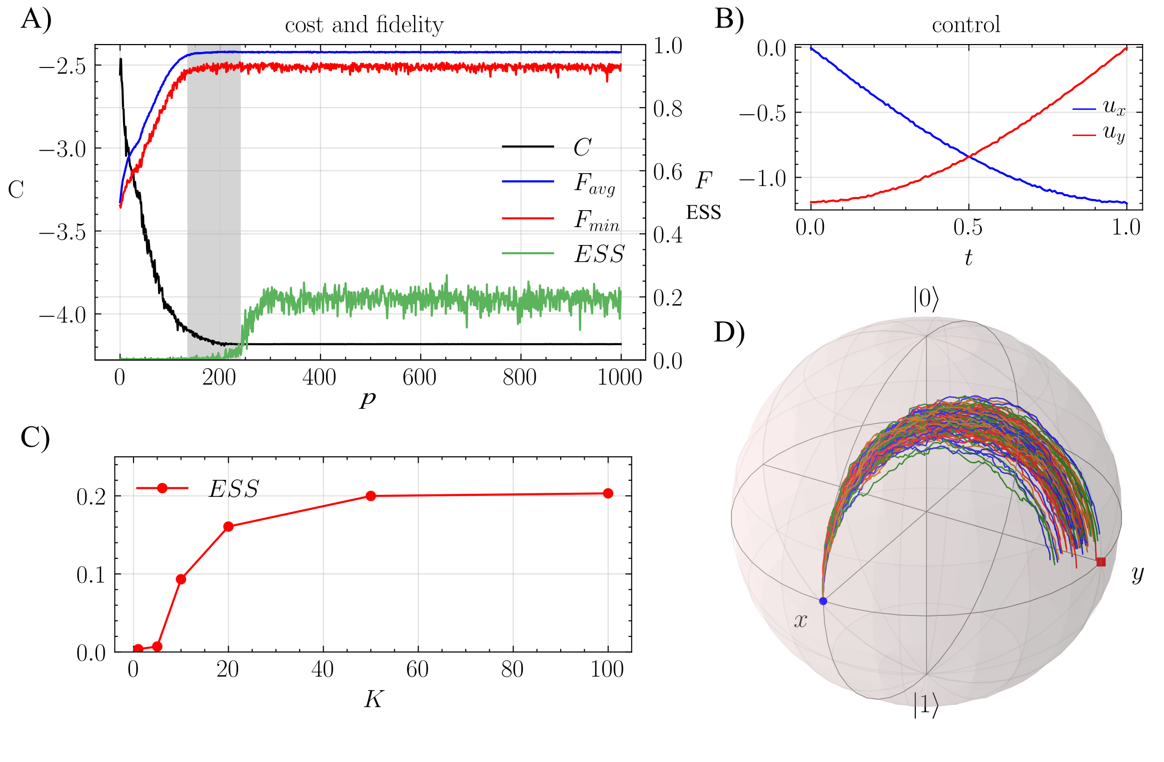
Figure 1: Control of a noise qubit from $X\to Y$. (A) Average fidelity $F_{\text{avg}}$, minimal fidelity $F_{\text{min}}$, effective sample size ESS and cost $C$ Eq. 19 versus importance sampling iterations $p$. The converged average fidelity is $F^{*}=0.9759\pm 0.0006$. (B) Optimal control solution $u_{x,y}(t)$ after convergence of the algorithm. The optimal solution is two-fold degenerate. The two solutions are related by a global sign $u_{x,y}\rightarrow-u_{x,y}$. (C). Dependence of the quality of the optimal control, measured by the ESS, on the number of pulses $K$. (D). Optimally controlled trajectories on the Bloch sphere. Parameters: horizon time $T=1$, noise coupling $D=0.005$, control weight $R=1$, fidelity weight $Q=10$, number of pulses $K=128$, number of trajectories $n_{traj}=400$ per IS step, maximum number of importance sampling (IS) steps $n_{IS}=1000$ and time discretization $dt=T/N$ with $N=128$. IS smoothing window $w=40$ (see section 3.1).

As benchmark, we compare the performances of PI control and (first order) Open GRAPE algorithm [28], which computes coherent controls for the Lindblad equation. See Appendix C for details on the algorithm and implementation. We solve the state preparation problem $X\rightarrow Y$ for the single qubit using $K=128$ pulses. The control problem is defined by the Lindblad equation (22) and the cost function (18).

We run PI and Open GRAPE algorithms 505 times using random control initializations drawn from both normal and uniform distributions. Regarding the stopping condition for Open GRAPE, the optimization stops when the cost cannot be further optimized by decreasing the learning rate; see App. C for details. In the case of PI algorithm, the optimization runs for a maximum of 800 IS steps, ensuring that the algorithm reaches convergence in every run.

In Fig. 2 we show the distribution of control costs (along the fidelities and fluences) for Open GRAPE (main panels) and PI (insets). We mark the average cost, fidelity and fluence of PI solutions by a yellow dot in each graph. The PI solutions have lower cost than the Open GRAPE solutions. The width of the dashed vertical lines locating each mean is much larger than the standard deviation of each PI distribution, showing that the variance of PI solutions is very narrow compared to that of Open GRAPE ones. Open GRAPE converges to many different solutions with different costs depending on the initial condition. Instead, PI control converges consistently to one of two solutions with same cost, fidelity, fluence and effective sample size, which are related by a global sign (Fig. 1 (B)). The difference between individual solutions has RMS error less than ${\cal O}\left({10^{-4}}\right)$. By direct inspection we can also verify that these profiles correspond to two different underlying smooth solutions. We conclude that the different PI solutions, rather than representing local minima, correspond to the same underlying solution up to small statistical fluctuations due to the stochastic nature of the algorithm.

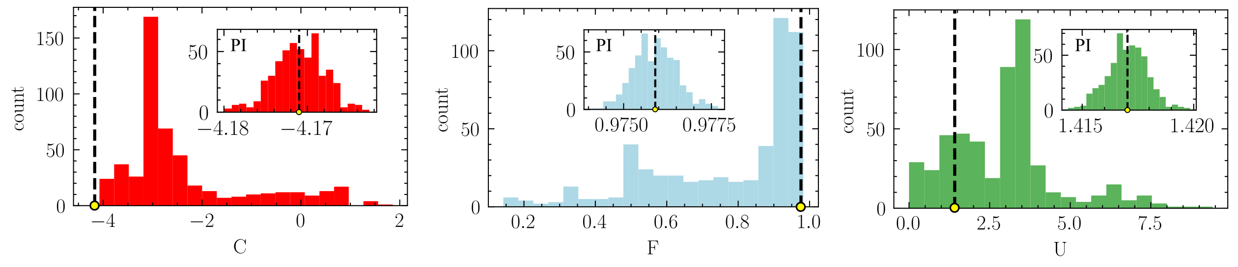
Figure 2: Histograms of optimal control costs obtained with Open GRAPE (main panel) and PI (inset) on $505$ runs. For Open GRAPE, the average cost, fidelity and fluence (and standard deviations) are $\left\langle C\right\rangle=-4\pm 1$, $\left\langle F\right\rangle=0.8\pm 0.2$ and $\left\langle U\right\rangle=3\pm 2$, respectively. The minimum cost achieved is $C_{min}=-4.07$. For PI, the corresponding average values (yellow dot) are $\left\langle C\right\rangle=-4.171\pm 0.003$, $\left\langle F\right\rangle=0.9759\pm 0.0006$ and $\left\langle U\right\rangle=1.4170\pm 0.0009$. In the main panels, the dashed vertical lines at the PI average are wider than the actual standard deviations of the PI distributions. This illustrates the large difference in variance between the two methods. All PI runs converge to solutions with the same cost, fidelity, fluence and effective sample size up to small statistical fluctuations due to the stochastic nature of PI control. Parameter setting: $D=0.005$, $T=1$, $R=1$, $Q=10,K=128$, $w=20$.

We further compare these two algorithms’ solutions by preforming a t-SNE embedding [82] over Open GRAPE solutions together with PI solutions. In Fig. 3 (A) we plot some of the most regular Open GRAPE control solutions. In Fig. 3 (B) we show the t-SNE embeddings for $[u_{x},u_{y}]$, considered as a vector of length $2K$. Each dot represent a different Open GRAPE solution and we represent the (average) PI solutions with yellow dots. We further perform a K-means decomposition to cluster the different solutions into 3 clusters (colored with red, blue and black). The different Open GRAPE solutions tend to cluster around each ground truth PI solution. In Fig. 3 (C) we plot the average profiles of the Open GRAPE solutions of cluster 1 (red) and cluster 2 (blue) together with the average PI profiles. The qualitative resemblance between the averages and the PI solution indicates that the Open GRAPE local minima tend to cluster around the ground truth solutions represented by PI solutions. The cluster colored with black consists of local minima control solution of Open GRAPE with high control cost $C$.

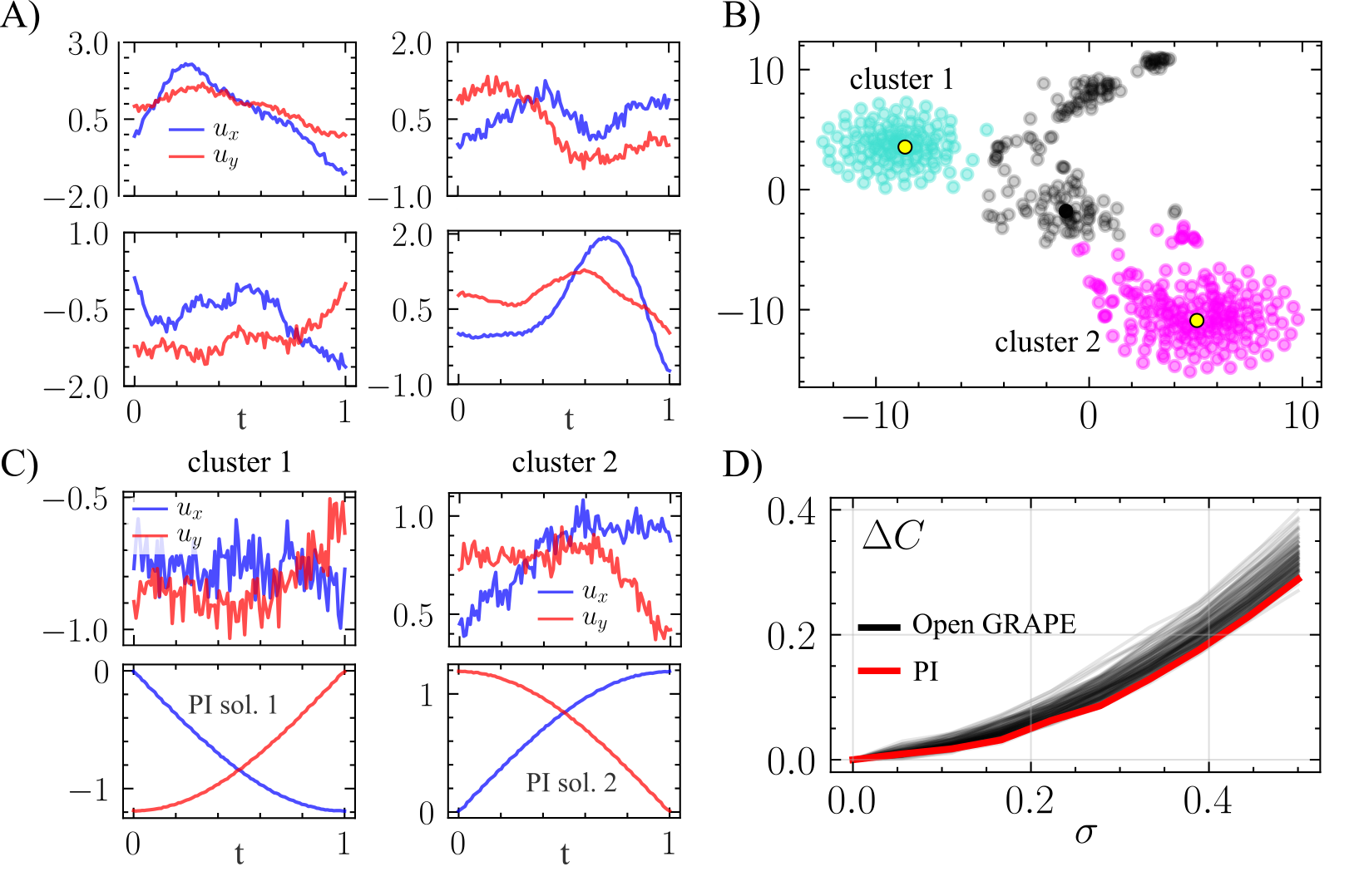
Figure 3: (A) Examples of Open GRAPE solutions with diverse levels of regularity for different seeds. (B) 2-D t-SNE dimension reduction representation followed by a K-means decomposition of Open GRAPE solutions (red, blue and black dots) and the two average PI solutions (yellow dots). The cluster of black dots correspond to local minima of relatively high cost $C$. (C) Average Open GRAPE solutions for cluster 1 (red) and cluster 2 (blue). In the bottom panels, the PI solutions corresponding to each cluster. (D) Robustness $\Delta C=C(u+\xi)-C(u)$ versus $\sigma$ with $u$ the high-fidelity high-ESS PI solution (red) and the high-fidelity low-ESS Open Grape solution (black).

During the IS iterations of the PI method, the optimization keeps improving in terms of ESS, even when maximum fidelities are reached; see shaded area in Fig. 1. Instead, Open GRAPE solutions, while having similar fidelities as the PI solution, have low $ESS={\cal O}\left({10^{-3}}\right)$. We expect that the high fidelity, high-ESS PI solutions are more robust to random perturbations than the high fidelity, low-ESS Open GRAPE solutions. We test this by perturbing the optimal control solution $u(t)\to u(t)+\xi(t)$ with $\xi(t)$ with Gaussian perturbations with mean zero and standard deviation $\sigma$ and compute the maximal cost difference $\Delta C=C(u+\xi)-C(u)$ for 20 different noise realizations. We compare high-fidelity low-ESS Open GRAPE solutions, defined by having a cost $C<-3.8$ with the high fidelity high ESS PI solution in Fig. 3 (D) for different $\sigma$. For completeness, we also include in the experiment the high-fidelity low-ESS PI solutions corresponding to the shaded area of Fig. 1 (A). It can be observed that the PI solution (in red) is more robust to random perturbations than low-ESS Open GRAPE solutions (in black). Therefore, we conclude that the ESS is a useful additional criterion to assess the quality in terms of the robustness of the (open loop) control solution.

5.2 The multi-qubit case

Consider a 1-D spin chain of $n$ qubits with single and pair-wise controls. Since this is a toy model designed to test the scalability of our algorithm for a larger number of qubits, we do not assert its feasibility in a lab setting, but rather emphasize the simplicity of defining such control problems within our framework. For simplicity, we set $H_{0}=0$. The control Hamiltonian is

$$H_{c}=\sum_{i=1}^{n}\sum_{a=x,y}u_{ia}\sigma_{i}^{a}+\sum_{i=1}^{n-1}\sum_{a,b=x,y}u_{iab}\sigma_{i}^{a}\sigma_{i+1}^{b}$$ (25)

where the controls $u_{ia}$ act on spin $i$, and controls $u_{iab}$ on the pair $i,\,i+1$. Note, that $H_{c}$ is an extension of typical NMR control Hamiltonians [83] with the addition of pair-wise controls.

The open dynamics is described by the Lindblad equation

$$\dot{\rho} =-i[H,\rho]+D_{1}\sum_{i=1}^{n}\left(\sigma_{i}^{-}\rho\sigma_{i}^{+}+\sigma^{+}_{i}\rho\sigma_{i}^{-}-\rho\right)+D_{2}\sum_{i=1}^{n-1}\sum_{v,w=\pm}\left(\sigma_{i}^{v}\sigma_{i+1}^{w}\rho\sigma_{i}^{-v}\sigma_{i+1}^{-w}-\rho\right)$$ (26)

with dissipation $\sigma^{\pm}$ of equal strength $D_{1}$ acting on individual spins and with strength $D_{2}$ on neighboring pairs of spins.

The control cost is defined as

$$C=\left\langle-\frac{Q}{2}{\cal F}(\psi_{T})+\frac{1}{2}\int_{0}^{T}\left(R_{1}\sum_{i=1}^{n}\sum_{a=x,y}u_{ia}^{2}+R_{2}\sum_{i=1}^{n-1}\sum_{a,b=x,y}u^{2}_{iab}\right)dt\right\rangle$$ (27)

Analogous to the previous section, we perform the transformation (23) to map non-Hermitian operators into anti-Hermitian. We transform the operators $C_{ia}=\sigma_{i}^{a},a=\pm$ and $C_{iab}=\sigma_{i}^{a}\sigma_{i+1}^{b},a,b=\pm$ in Eq. (26) into anti-Hermitian operators

$$\tilde{C}_{ib}=C_{ia}A_{ab}\qquad\tilde{C}_{icd}=C_{iab}A_{abcd}\qquad\text{for all $i$}$$ (28)

with $A_{abcd}:=iA_{ac}A_{bd}$. This leads to the following expression for the transformed operators

$$\tilde{C}_{ib}=-i\sigma_{i}^{b}\qquad\tilde{C}_{icd}=-i\sigma_{i}^{c}\sigma_{i+1}^{d}\qquad\text{for all $i$\,\, and \,\,$b,c,d=x,y$}\,.$$ (29)

and $\tilde{D}_{1}=\frac{1}{2}D_{1},\tilde{D}_{2}=\frac{1}{4}D_{2}$.

The corresponding unraveling is

$$d\psi=-i\left(\sum_{i=1}^{n}\sum_{a=x,y}(u_{ia}dt+dW_{ia})\sigma_{i}^{a}+\sum_{i=1}^{n-1}\sum_{a,b=x,y}(u_{iab}dt+dW_{iab})\sigma_{i}^{a}\sigma_{i+1}^{b}\right)\psi dt-\left(n\tilde{D}_{1}+2(n-1)\tilde{D}_{2}\right)\psi dt$$ (30)

with $\left\langle d\tilde{W}_{ia}d\tilde{W}_{jb}\right\rangle=\delta_{ij}\delta_{ab}\tilde{D}_{1}dt$ for $i,j=1,\dots n$ and $a,b=x,y$, and $\left\langle d\tilde{W}_{iab}d\tilde{W}_{jcd}\right\rangle=\delta_{ij}\delta_{ac}\delta_{bd}\tilde{D}_{2}dt$ for $i,j=1,\ldots,n-1$ and $a,b,c,d=x,y$. Equations (27) and (30) define a path integral control problem when

$$\lambda=\tilde{D}_{1}R_{1}=\tilde{D}_{2}R_{2}$$ (31)

The initial state is $\psi_{0}=\ket{0}^{n}$. We choose the target state $\phi$ to be a Greenberger–Horne–Zeilinger (GHZ) state, which is defined as $\ket{GHZ_{n}}:=\frac{1}{\sqrt{2}}\left(\ket{0}^{n}+\ket{1}^{n}\right)$ for $n$-qubit systems and it represents a maximally entangled state in the global entanglement (or Meyer-Wallach) measure for multipartite systems [84]. We set $R_{1}=R_{2}=R/{n_{c}}$ with $n_{c}=2n+4(n-1)$ the total number of controls. This normalization defines a fluence cost per unit control. The path integral condition Eq. 31 then implies that $\tilde{D}_{2}=\tilde{D}_{1}$ or $D_{2}=2D_{1}$. We take as free parameters $R$ and $D_{1}$. We run the algorithm for $n=10$ qubits. The results are shown in Fig. 4, showing the usefulness of the PI method for relatively large systems. Note, a direct implementation of this problem in Open GRAPE would require to compute and store matrix exponentials of size $N^{2}\times N^{2}$ at each step $K$, which is memory intensive and requires an efficient implementation of the algorithm (see for example [28, 85]) and/or dedicated software. Our PI quantum control algorithm runs in a desktop computer.

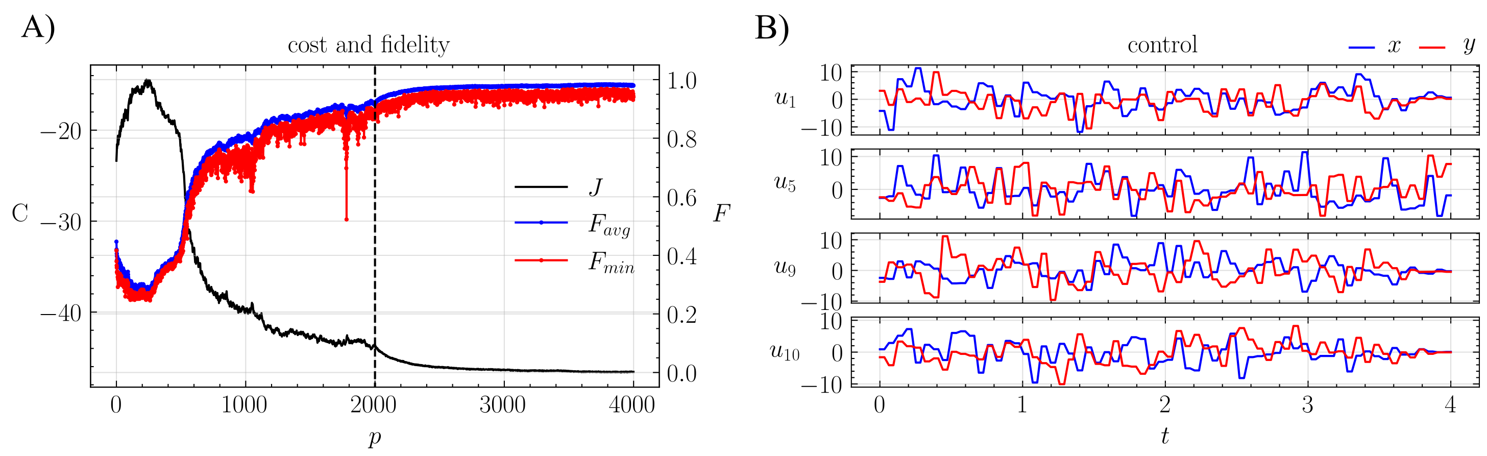
Figure 4: Control of a $n=10$ qubit 1-D spin chain. The IS training (panel A) has two parts (marked by the vertical dashed line), where in the first part we set the IS window $w=1$ (no smoothing), and in the second part we change it to $w=10$. This is to speedup convergence in the first part, and later to improve the statistics. The average fidelity reached $F_{avg}=0.982\pm 0.001$. Runtime $\sim 6.8$hr on a desktop computer. In panel (B) we illustrate the control solutions for qubits 1, 5, 9 and 10. The $x$/$y$ components of each control are marked by blue and red colors, respectively. The parameters are $K=64$, $T=4$, $R$=0.1, $D=0.001$, $Q$=100, $n_{IS}$=4000, and $n_{traj}$=100.

6 Discussion

In this work we propose a novel approach for optimal control of open quantum systems. We bring together tools from path integral control and quantum trajectories to frame a broad class of quantum control problems in the language of stochastic optimal control theory. Stochastic optimal control problems usually demand the integration of a Hamilton-Jacobi-Bellman equation, which is prohibitive for large systems. PI control bypasses this requirement giving the optimal solution explicitly as a path integral. Optimal controls are then computed by sampling stochastic trajectories in the Hilbert space. The PI formulation of the control problem readily enables the integration of Monte Carlo and Machine Learning techniques into the estimation process. In this work, we use iterative importance sampling, a scheme where the controls are incrementally improved and the optimal control solutions are seen as fixed points of this process.

The main features of our method can be summarized as follows: 1) it is state-centered: the quantum trajectories are obtained by propagating state vectors of size $N$, opposed to most common density-based approaches, which require density matrices of size $N^{2}$; in this way, our algorithm inherently comprises a quadratic advantage in runtime over density-based methods, such as the PMP method or the adjoint method [32]. 2) it is embarrassingly parallel: The core of the PI control computation is to learn a model on the basis of self-generated data (sample trajectories) and this procedure is iterated using improved controllers until convergence. The importance sampling updates Eqs. (14) and (16) can be very efficiently parallelized by noting that the gradient consists of a sum over the data and that the computation of this sum can be distributed over $n$ machines so that the updated parameters $\theta_{p+1}=\theta_{p}+\frac{1}{n}\sum_{i=1}^{n}d\theta_{p}^{(i)}$ with $d\theta_{p}^{(i)}$ the gradient update computed on machine $i$. No large volumes of simulated raw data need to be transferred between machines, only the parameter updates. See fig. 5. This results in close-to-linear speedup.

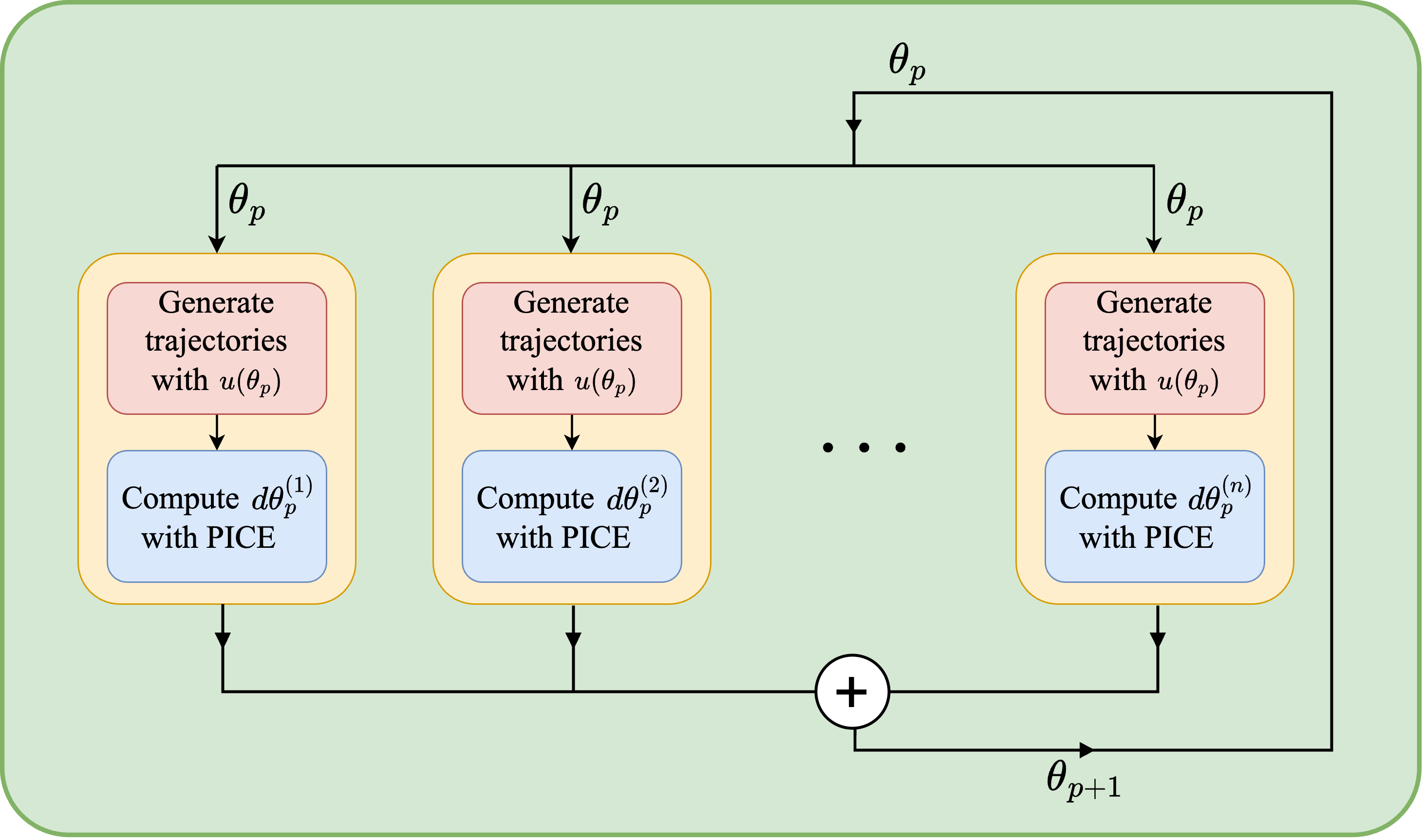
Figure 5: During each iteration, samples are generated using control functions $u(\theta_{p})$. These samples are used to compute new parameters $\theta_{p+1}$. These two steps can be distributed on many machines with minimal communication overhead, since no large volumes of simulated raw data need to be transferred between machines, only the parameter updates.

3) An important point concerns the nature of control computation in PI control. For any control problem, the primary computational challenge is to account for how early control actions influence the system’s state and cost at later times. For instance, GRAPE and PMP use some form of backward evolution of the co-state to estimate this dependence. PI control, instead, uses an entirely different mechanism, by generating forward sampled stochastic particle trajectories that are weighted with their exponentiated control cost. These global statistics are then used to update the parameters in each time bin independently. This is a prominent feature of our PI control algorithm and stands out from other methods where a direct access to the objective gradients is needed. Our experiments show that this is a more effective way to compute the optimal control solution, when the control problem is of the PI form.

For linear parametrizations, either open-loop or feedback, the importance sampling updates are computed as stochastic averages as given by Eqs. (14) and (16). For non-linear parametrizations, for instance when the control functions $u(\theta)$ are represented by deep neural networks, a more general iterative importance sampling algorithm is given by the Path integral Cross-Entropy (PICE) method [86], involving the gradients $\partial u/\partial\theta$. As in any neural network training, these gradients can be computed using automatic differentiation [87].

In this paper we have used the PI control method to computed open loop control solutions to open quantum systems. The approach, including the importance sampling methods and their generalization to PICE, automatically generalize to compute feed back control solutions. However, the feedback controller requires information about the quantum state through measurement. Since the quantum state is only partially observable through measurement, the control problem becomes what is known as a partial observable control problem [63]. A unique quantum feature, not present in classical systems, is that measurement will disrupt the quantum state by projecting the state onto one of the measurement eigenstates (quantum back-action). A compromise between information gain and minimal disruption of the quantum state is given by the the so-called weak or continuous measurement [64, 65, 66]. Weak measurement can be elegantly formalized by the so-called hybrid dynamics, which describes the simultaneous time evolution of the quantum state and the classical observation(s) [67, 69, 70]. The extension of our approach to incorporate partial observation and measurement is currently under development and will be presented in future work.

Appendix A Unraveling calculations

Proof.

Proof of Theorem 1. Consider the stochastic dynamics

$$d\psi=-iH^{\prime}\psi dt-\frac{1}{2}D_{ab}{C^{\prime}_{b}}^{\dagger}C^{\prime}_{a}\psi dt+C^{\prime}_{a}\psi dW^{a}$$ (32)

with $\left\langle dW_{a}dW_{b}\right\rangle=D_{ab}dt$ and $H^{\prime},C^{\prime}$ to be defined later. Define the quantum state $P=\psi\psi^{\dagger}$. Then using Ito calculus, the dynamics of $P$ is

$$dP=d\psi\psi^{\dagger}+\psi d\psi^{\dagger}+d\psi d\psi^{\dagger}=-i[H^{\prime},P]dt+{\cal D}[C^{\prime},D](P)dt+[C^{\prime}_{a}PdW_{a}+h.c.]$$ (33)

$\psi$ is a stochastic vector with norm $\|\psi\|^{2}=\psi^{\dagger}\psi$. Using Ito calculus, the change in the norm is given by

$$d\left(\|\psi\|^{2}\right)=d\psi^{\dagger}\psi+\psi^{\dagger}d\psi+d\psi^{\dagger}d\psi=\psi^{\dagger}(C^{\prime}_{a}+(C^{\prime}_{a})^{\dagger})\psi dW_{a}$$ (34)

We can ensure that $\|\psi\|^{2}$ is conserved by defining $C^{\prime}_{a}=C_{a}-c_{a}$ with $c_{a}=\psi^{\dagger}C^{(h)}_{a}\psi$ and $C_{a}^{(h)}$ the Hermitian part of $C_{a}$. Note, that $c_{a}$ is real. With this choice Eqs. (32) and (33) become

$$d\psi = -iH^{\prime}\psi dt-\frac{1}{2}D_{ab}(C_{b}-c_{b})^{\dagger}(C_{a}-c_{a})\psi dt+(C_{a}-c_{a})\psi dW_{a}$$ (35)

$$dP = -i[H^{\prime}-iD_{ab}c_{a}C_{b}^{(ah)},P]+{\cal D}[C,D](P)dt+[(C_{a}-c_{a})PdW_{a}+h.c.]$$ (36)

with $C_{a}^{(ah)}=\frac{1}{2}(C_{a}-C_{a}^{\dagger})$. To connect to the Lindblad equation, define $H=H^{\prime}-iD_{ab}c_{a}C^{(ah)}_{b}$. Then substitution in (35) and (36) yields (2) and

$$dP=-i[H,P]dt+{\cal D}[C,D](P)dt+[(C_{a}-c_{a})PdW_{a}+h.c.]$$ (37)

Define $\rho:=\left<P\right>$ and $\left<dP\right>:=\dot{\rho}dt$. Taking the average of (37) yields the Lindblad equation (1), which completes the proof. ∎

Appendix B Path integral control theory

In this section we describe some basic results regarding PI control theory. For further details the reader may consult the original papers [88, 89].

Define

$$\psi(t,x)=e^{-J(t,x)/\lambda}\qquad\phi(t)=e^{(S^{u}(t)-S^{u}(t_{0}))/\lambda}$$

where $\lambda I=R\nu$. Furthermore we define the stochastic processes $\psi(t)=\psi(t,X_{t}^{u}),u(t)=u(t,X_{t}^{u})$ and $u^{*}(t)=u^{*}(t,X_{t}^{u})$

Lemma 3.

For all $t$ in $t_{0}\leq t\leq t_{1}$

$$e^{-S^{u}(t)/\lambda}-\psi(t)=\frac{1}{\lambda\phi(t)}\int_{t}^{t_{1}}\phi(s)\psi(s)(u^{*}(s)-u(s))^{T}RdW_{s}$$ (38)

Proof.

Define the optimal cost-to-go as the minimal expected cost starting in any $x$ at time $t$ with $t_{0}\leq t\leq t_{1}$

$$J(t,x) = \min_{u}\left<S^{u}(t)\right>_{X^{u}_{t}=x}\qquad u^{*}(t,x)=\underset{u}{\text{argmin}}\left<S^{u}(t)\right>_{X^{u}_{t}=x}$$ (39)

where the minimization is over all smooth functions $u(\cdot,s),t\leq s\leq t_{1}$. The HJB equation for the control problem Eqs. (6) and (7) is

$$-J_{t}=\min_{u}\left(V+\frac{1}{2}u^{T}Ru+(f+gu)^{T}J_{x}+\frac{1}{2}\mathrm{Tr}(g\nu g^{T}J_{xx})\right)$$

where subscripts $t,x$ denote differentiation with respect to $t,x$ and with boundary condition $J(t_{1},x)=\Phi(x)$. We can solve for $u$, which gives $u^{*}=-R^{-1}g^{T}J_{x}$ and

$$-J_{t}=V-\frac{1}{2}J_{x}^{T}gR^{-1}g^{T}J_{x}+f^{T}J_{x}+\frac{1}{2}\mathrm{Tr}(g\nu g^{T}J_{xx})$$ (40)

We assume that the matrices $R,\nu$ are related such that $R=\lambda\nu^{-1}$ with $\lambda>0$. In terms of $\psi$, Eq. (40) becomes linear

$$\psi_{t}+f^{T}\psi_{x}+\frac{1}{2}\mathrm{Tr}(g\nu g^{T}\psi_{xx})=\frac{V}{\lambda}\psi$$ (41)

Alternatively, we consider the stochastic process $\psi(t)=\psi(t,X_{t}^{u})$. Using $\hat{I}$to calculus we obtain

$$d\psi = \left(\psi_{t}+\psi_{x}^{T}(f+gu)+\frac{1}{2}\mathrm{Tr}(g\nu g^{T}\psi_{xx})\right)dt+\psi_{x}^{T}gdW=\frac{V}{\lambda}\psi+\psi_{x}^{T}g(udt+dW)$$

where we used Eq. (41), with boundary condition $\psi(t_{1},x)=e^{-\Phi(x)/\lambda}$. Using the definition of $\phi(t)$ we obtain

$$d\phi=-\frac{1}{\lambda}\left(Vdt+u^{T}RdW\right)$$

with initial condition $\phi(t_{0})=1$. Using the product rule we obtain

$$d(\phi\psi)=d\phi\psi+\phi d\psi+d[\phi,\psi]=-\frac{1}{\lambda}\psi\phi u^{T}RdW+\phi\psi_{x}^{T}gdW=\frac{1}{\lambda}\phi\psi(u^{*}-u)^{T}RdW$$

where in the last step we used $u^{*}=\lambda R^{-1}g^{T}\frac{\psi_{x}}{\psi}$. Integrating from $t$ to $t_{1}$ we obtain

$$\phi(t_{1})\psi(t_{1})-\phi(t)\psi(t)=\frac{1}{\lambda}\int_{t}^{t_{1}}\phi(s)\psi(s)(u^{*}(s)-u(s))^{T}RdW_{s}$$

We use $\phi(t_{1})=\phi(t)e^{(S^{u}(t_{1})-S^{u}(t))/\lambda}$ and divide by $\phi(t)$ to obtain Eq. (38). ∎

Corollary 4.

We take the expectation of Eq. (38) with respect to $dW_{t:t_{1}}$ and condition on events up to time $t$, which we call a filtration ${\cal F}_{t}$, we obtain

$$\psi(t)=\left<e^{-S^{u}(t)/\lambda}\right>_{{\cal F}_{t}}$$ (42)

The following path integral control theorem is useful to estimate these parameters for all times from one set of samples $X^{u}_{t_{0}:t_{1}}$.

Theorem 5.

Let $f:\mathbb{R}\times\mathbb{R}^{n}\to\mathbb{R}$ and define the process $f_{t}=f(t,X^{u}_{t})$. Then

$$\left<e^{-S^{u}(t_{0})/\lambda}\int_{t_{0}}^{t_{1}}(u^{*}(s)-u(s))f(s)ds\right>=\left<e^{-S^{u}(t_{0})/\lambda}\int_{t_{0}}^{t_{1}}f(s)dW_{s}\right>$$ (43)

where the expectation is with respect to the stochastic process (6).

Proof.

Consider Lemma (38) for $t=t_{0}$. Multiply both sides by $\int_{t_{0}}^{t_{1}}f(s)dW_{s}$ and take the expectation value

$$\left\langle e^{-S^{u}(t_{0})}\int_{t_{0}}^{t_{1}}f(s)dW_{s}\right\rangle=\left\langle\int_{t_{0}}^{t_{1}}f(s)dW_{s}\int_{t_{0}}^{t_{1}}\phi(s^{\prime})\psi(s^{\prime})(u^{*}(s^{\prime})-u(s^{\prime}))^{T}\frac{R}{\lambda}dW_{s^{\prime}}\right\rangle$$ (44)

Using $RD=\lambda$ and Ito isometry we have

$$\left\langle e^{-S^{u}(t_{0})}\int_{t_{0}}^{t_{1}}f(s)dW_{s}\right\rangle=\int_{t_{0}}^{t_{1}}\left\langle f(s)\phi(s)\psi(s)(u^{*}(s)-u(s))\right\rangle ds$$ (45)

Using the definition of $\psi(s)$ and $\phi(s)$ we write

$$\left\langle e^{-S^{u}(t_{0})}\int_{t_{0}}^{t_{1}}f(s)dW_{s}\right\rangle=\int_{t_{0}}^{t_{1}}\left\langle f(s)e^{(S^{u}(s)-S^{u}(t_{0}))/\lambda}\left\langle e^{-S^{u}(t_{0})}\right\rangle_{{\cal F}_{s}}(u^{*}(s)-u(s))\right\rangle ds$$ (46)

Finally, by applying the law of total expectation we obtain (43).

∎

Corollary 6.

By setting $f(t)=\delta_{t\in I}$ with $I=[t_{0},t_{0}+dt]$, diving by $dt$ and taking the limit $dt\rightarrow 0$ we establish the proof of (10).

Appendix C Open GRAPE

Here we summarize the details of our implementation of Open GRAPE for the benchmarking part of section 5.1. For further details concerning the definition of Open GRAPE algorithm we refer the reader to [28]. Given the cost objective (18) and the control model Eq. 12 with $R$ a positive scalar, the first order Open GRAPE update rule (ignoring terms of ${\cal O}(dt^{2})$ and higher) becomes

$$A_{ak}\rightarrow A^{\prime}_{ak}=A_{ak}-\varepsilon\frac{\partial C}{\partial A_{ak}}$$

with

$$\frac{\partial C}{\partial A_{ak}}=\frac{iQ}{2}\text{Tr}\left(\lambda_{k}[H_{a},\rho_{k}]\right)dt+RA_{ak}dt$$

where $\rho_{k}$ is the forward-propagated state from $\rho_{0}$ to time $t_{k}$ and $\lambda_{k}$ is the backward-propagated state from $\rho_{target}$ to time $t_{k}$, $\varepsilon$ is the learning rate, and $dt$ is the time step. We implement the algorithm in Python language. For the dynamics simulation of the backward and forward propagations we use the open-source Python package dynamiqs [90].

The learning rate $\varepsilon$ usually needs to be carefully chosen in order to avoid overshooting. In the case of GRAPE for closed systems, work [91] reported an adaptive learning rate at each $j$ step of $\varepsilon/j^{\alpha}$ with $\alpha=1/2$ was enough to avoid overshooting of local minima/saddle points. We found this approach not suitable for our benchmarking purposes as it required an excessive fine tuning of $\alpha$ for different types of seeds. We choose instead the following protocol: every time the cost $C(A^{\prime})\geq C(A)$, where $A$ the current solution and $A^{\prime}$ the new solution, the learning rate is reduced by a factor $10$ and $C(A^{\prime})$ is recomputed until either $C(A^{\prime})<C(A)$ or $\varepsilon$ is reduced a maximum number of times that we set to $10$. This stopping condition allows us to capture local minima and detect when the first order approximation of the gradient update starts to fail. At the start of each run, we sample random seeds $u$ from Gaussian distributions (centered at zero, 1, and -1, with standard deviation 2) and uniform distributions (integers between -10 and 10, with a scale factor of 1 and 0.5).

References

- [1] Lidar, D. A. & Brun, T. A. Quantum error correction (Cambridge university press, 2013).
- [2] Georgescu, I. M., Ashhab, S. & Nori, F. Quantum simulation. Reviews of Modern Physics 86, 153–185 (2014).
- [3] Giovannetti, V., Lloyd, S. & Maccone, L. Advances in quantum metrology. Nature photonics 5, 222–229 (2011).
- [4] Degen, C. L., Reinhard, F. & Cappellaro, P. Quantum sensing. Reviews of modern physics 89, 035002 (2017).
- [5] Arrazola, J. M. et al. Quantum circuits with many photons on a programmable nanophotonic chip. Nature 591, 54–60 (2021).
- [6] Hermans, S. et al. Qubit teleportation between non-neighbouring nodes in a quantum network. Nature 605, 663–668 (2022).
- [7] Baßler, P. et al. Synthesis of and compilation with time-optimal multi-qubit gates. Quantum 7, 984 (2023).
- [8] Bushev, P. et al. Feedback Cooling of a Single Trapped Ion. Physical Review Letters 96, 043003 (2006). URL https://link.aps.org/doi/10.1103/PhysRevLett.96.043003.
- [9] Rossi, M., Mason, D., Chen, J., Tsaturyan, Y. & Schliesser, A. Measurement-based quantum control of mechanical motion. Nature 563, 53–58 (2018). URL https://www.nature.com/articles/s41586-018-0643-8. Publisher: Nature Publishing Group.
- [10] Adams, C. S., Pritchard, J. D. & Shaffer, J. P. Rydberg atom quantum technologies. Journal of Physics B: Atomic, Molecular and Optical Physics 53, 012002 (2019).
- [11] Henriet, L. et al. Quantum computing with neutral atoms. Quantum 4, 327 (2020).
- [12] Magrini, L. et al. Real-time optimal quantum control of mechanical motion at room temperature. Nature 595, 373–377 (2021). URL https://www.nature.com/articles/s41586-021-03602-3. Publisher: Nature Publishing Group.
- [13] Cong, S. Control of quantum systems: theory and methods (John Wiley & Sons, 2014).
- [14] d’Alessandro, D. Introduction to quantum control and dynamics (Chapman and hall/CRC, 2021).
- [15] Mahesh, T., Batra, P. & Ram, M. H. Quantum optimal control: Practical aspects and diverse methods. Journal of the Indian Institute of Science 103, 591–607 (2023).
- [16] Khaneja, N., Reiss, T., Kehlet, C., Schulte-Herbrüggen, T. & Glaser, S. J. Optimal control of coupled spin dynamics: design of nmr pulse sequences by gradient ascent algorithms. Journal of magnetic resonance 172, 296–305 (2005).
- [17] Chen, Y. et al. Accelerating quantum optimal control through iterative gradient-ascent pulse engineering. Physical Review A 108, 052603 (2023). URL https://link.aps.org/doi/10.1103/PhysRevA.108.052603. Publisher: American Physical Society.
- [18] Caneva, T., Calarco, T. & Montangero, S. Chopped random-basis quantum optimization. Physical Review A 84, 022326 (2011).
- [19] Krotov, V. F. Global methods in optimal control theory. In Advances in nonlinear dynamics and control: a report from Russia, 74–121 (Springer, 1996).
- [20] Tannor, D., Kazakov, V., Orlov, V., Broeckhove, J. & Lathouwers, L. Time-dependent quantum molecular dynamics. Nato ASI Series B 299, 347 (1992).
- [21] Zhu, W., Botina, J. & Rabitz, H. Rapidly convergent iteration methods for quantum optimal control of population. The Journal of Chemical Physics 108, 1953–1963 (1998).
- [22] Boscain, U., Sigalotti, M. & Sugny, D. Introduction to the Pontryagin Maximum Principle for Quantum Optimal Control. PRX Quantum 2, 030203 (2021). URL http://arxiv.org/abs/2010.09368. 2010.09368.
- [23] Glaser, S. J. et al. Training Schrödinger’s cat: Quantum optimal control: Strategic report on current status, visions and goals for research in Europe. The European Physical Journal D 69, 279 (2015). URL http://link.springer.com/10.1140/epjd/e2015-60464-1.
- [24] Koch, C. P. et al. Quantum optimal control in quantum technologies. Strategic report on current status, visions and goals for research in Europe. EPJ Quantum Technology 9, 19 (2022). URL https://epjquantumtechnology.springeropen.com/articles/10.1140/epjqt/s40507-022-00138-x.
- [25] Davies, E. B. Quantum theory of open systems (Academic Press London, 1976).
- [26] Lindblad, G. On the generators of quantum dynamical semigroups. Communications in mathematical physics 48, 119–130 (1976).
- [27] Breuer, H.-P. & Petruccione, F. The theory of open quantum systems (Oxford University Press, USA, 2002).
- [28] Boutin, S., Andersen, C. K., Venkatraman, J., Ferris, A. J. & Blais, A. Resonator reset in circuit qed by optimal control for large open quantum systems. Physical Review A 96, 042315 (2017).
- [29] Schmidt, R., Negretti, A., Ankerhold, J., Calarco, T. & Stockburger, J. T. Optimal control of open quantum systems: Cooperative effects of driving and dissipation. Phys. Rev. Lett. 107, 130404 (2011). URL https://link.aps.org/doi/10.1103/PhysRevLett.107.130404.
- [30] Hwang, B. & Goan, H.-S. Optimal control for non-markovian open quantum systems. Physical Review A 85, 032321 (2012).
- [31] Goerz, M. H. & Jacobs, K. Efficient optimization of state preparation in quantum networks using quantum trajectories. Quantum Science and Technology 3, 045005 (2018).
- [32] Gautier, R., Genois, É. & Blais, A. Optimal control in large open quantum systems: The case of transmon readout and reset (2024). 2403.14765.
- [33] Murray, D. & Yakowitz, S. Differential dynamic programming and newton’s method for discrete optimal control problems. Journal of Optimization Theory and Applications 43, 395–414 (1984).
- [34] Davies, E. B. Quantum stochastic processes. Communications in Mathematical Physics 15, 277–304 (1969).
- [35] Carmichael, H. An Open Systems Approach to Quantum Optics: Lectures Presented at the Université Libre de Bruxelles October 28 to November 4, 1991, vol. 18 of Lecture Notes in Physics Monographs (Springer, Berlin, Heidelberg, 1993). URL http://link.springer.com/10.1007/978-3-540-47620-7.
- [36] Percival, I. Quantum state diffusion (Cambridge University Press, 1998).
- [37] Daley, A. J. Quantum trajectories and open many-body quantum systems. Advances in Physics 63, 77–149 (2014). 1405.6694.
- [38] Wiseman, H. M. & Diósi, L. Complete parameterization, and invariance, of diffusive quantum trajectories for Markovian open systems. Chemical Physics 268, 91–104 (2001). quant-ph/0012016.
- [39] Dalibard, J., Castin, Y. & Mølmer, K. Wave-function approach to dissipative processes in quantum optics. Physical review letters 68, 580 (1992).
- [40] Dum, R., Zoller, P. & Ritsch, H. Monte carlo simulation of the atomic master equation for spontaneous emission. Physical Review A 45, 4879 (1992).
- [41] Gisin, N. & Percival, I. C. The quantum-state diffusion model applied to open systems. Journal of Physics A: Mathematical and General 25, 5677 (1992).
- [42] Barchielli, A. & Gregoratti, M. Quantum Trajectories and Measurements in Continuous Time: The Diffusive Case, vol. 782 of Lecture Notes in Physics (Springer Berlin Heidelberg, Berlin, Heidelberg, 2009).
- [43] Hudson, R. L. & Parthasarathy, K. R. Quantum Itô’s formula and stochastic evolutions. Communications in mathematical physics 93, 301–323 (1984).
- [44] Parthasarathy, K. R. An introduction to quantum stochastic calculus, vol. 85 (Birkhäuser, 2012).
- [45] Belavkin, V., Hirota, O. & Hudson, R. L. Quantum communications and measurement (Springer Science & Business Media, 2013).
- [46] Barchielli, A. & Belavkin, V. P. Measurements continuous in time and a posteriori states in quantum mechanics. Journal of Physics A: Mathematical and General 24, 1495 (1991).
- [47] Diósi, L. & Strunz, W. T. The non-markovian stochastic schrödinger equation for open systems. Physics Letters A 235, 569–573 (1997).
- [48] Gambetta, J. & Wiseman, H. M. Non-markovian stochastic schrödinger equations: Generalization to real-valued noise using quantum-measurement theory. Physical Review A 66, 012108 (2002).
- [49] Murch, K. W., Weber, S. J., Macklin, C. & Siddiqi, I. Observing single quantum trajectories of a superconducting quantum bit. Nature 502, 211–214 (2013). URL https://www.nature.com/articles/nature12539. Publisher: Nature Publishing Group.
- [50] Campagne-Ibarcq, P. et al. Observing Quantum State Diffusion by Heterodyne Detection of Fluorescence. Physical Review X 6, 011002 (2016). URL https://link.aps.org/doi/10.1103/PhysRevX.6.011002. Publisher: American Physical Society.
- [51] Ficheux, Q., Jezouin, S., Leghtas, Z. & Huard, B. Dynamics of a qubit while simultaneously monitoring its relaxation and dephasing. Nature Communications 9, 1926 (2018). URL https://www.nature.com/articles/s41467-018-04372-9. Publisher: Nature Publishing Group.
- [52] Minev, Z. K. et al. To catch and reverse a quantum jump mid-flight. Nature 570, 200–204 (2019). URL https://www.nature.com/articles/s41586-019-1287-z. Publisher: Nature Publishing Group.
- [53] Wieczorek, W. et al. Optimal State Estimation for Cavity Optomechanical Systems. Physical Review Letters 114, 223601 (2015). URL https://link.aps.org/doi/10.1103/PhysRevLett.114.223601. Publisher: American Physical Society.
- [54] Rossi, M., Mason, D., Chen, J. & Schliesser, A. Observing and Verifying the Quantum Trajectory of a Mechanical Resonator. Physical Review Letters 123, 163601 (2019). URL https://link.aps.org/doi/10.1103/PhysRevLett.123.163601.
- [55] Thomas, R. A. et al. Entanglement between distant macroscopic mechanical and spin systems. Nature Physics 17, 228–233 (2021). URL https://www.nature.com/articles/s41567-020-1031-5. Publisher: Nature Publishing Group.
- [56] Wiseman, H. M. & Milburn, G. J. Quantum theory of optical feedback via homodyne detection. Physical Review Letters 70, 548 (1993).
- [57] Belavkin, V. Theory of the control of observable quantum systems. Automatica and Remote Control 44, 178–188 (1983).
- [58] Wiseman, H. M. & Milburn, G. J. Quantum measurement and control (Cambridge university press, 2009).
- [59] Pham, H. Continuous-time stochastic control and optimization with financial applications, vol. 61 (Springer Science & Business Media, 2009).
- [60] Yong, J. & Zhou, X. Stochastic controls. Hamiltonian Systems and HJB Equations (Springer, 1999).
- [61] Doherty, A. C. & Jacobs, K. Feedback control of quantum systems using continuous state estimation. Physical Review A 60, 2700–2711 (1999). URL https://link.aps.org/doi/10.1103/PhysRevA.60.2700.
- [62] Doherty, A. C., Habib, S., Jacobs, K., Mabuchi, H. & Tan, S. M. Quantum feedback control and classical control theory. Physical Review A - Atomic, Molecular, and Optical Physics 62, 13 (2000). quant-ph/9912107.
- [63] Bensoussan, A. Stochastic control of partially observable systems (Cambridge University Press, 1992).
- [64] Kraus, K., Böhm, A., Dollard, J. D. & Wootters, W. States, Effects, and Operations Fundamental Notions of Quantum Theory: Lectures in Mathematical Physics at the University of Texas at Austin (Springer, 1983).
- [65] Aharonov, Y., Albert, D. Z. & Vaidman, L. How the result of a measurement of a component of the spin of a spin- 1/2 particle can turn out to be 100. Physical Review Letters 60, 1351–1354 (1988). URL https://link.aps.org/doi/10.1103/PhysRevLett.60.1351.
- [66] Hatridge, M. et al. Quantum back-action of an individual variable-strength measurement. Science 339, 178–181 (2013).
- [67] Aleksandrov, I. V. The Statistical Dynamics of a System Consisting of a Classical and a Quantum Subsystem. Zeitschrift für Naturforschung A 36, 902–908 (1981). URL https://www.degruyter.com/document/doi/10.1515/zna-1981-0819/html. Publisher: De Gruyter.
- [68] Blanchard, P. & Jadczyk, A. Events and piecewise deterministic dynamics in event-enhanced quantum theory. Physics Letters A 203, 260–266 (1995). URL https://www.sciencedirect.com/science/article/pii/0375960195004323.
- [69] Layton, I., Oppenheim, J. & Weller-Davies, Z. A healthier semi-classical dynamics (2023). URL http://arxiv.org/abs/2208.11722. ArXiv:2208.11722 [gr-qc, physics:hep-th, physics:quant-ph].
- [70] Diósi, L. Hybrid completely positive Markovian quantum-classical dynamics. Physical Review A 107, 062206 (2023). URL https://link.aps.org/doi/10.1103/PhysRevA.107.062206. Publisher: American Physical Society.
- [71] Gisin, N. Quantum Measurements and Stochastic Processes. Physical Review Letters 52, 1657–1660 (1984). URL https://link.aps.org/doi/10.1103/PhysRevLett.52.1657. Publisher: American Physical Society.
- [72] Diósi, L. Continuous quantum measurement and It\^o formalism. Physics Letters A 129, 419–423 (1988). URL http://arxiv.org/abs/1812.11591. ArXiv:1812.11591 [quant-ph].
- [73] Kappen, H. Linear theory for control of non-linear stochastic systems. Physical Review letters 95, 200201 (2005).
- [74] Kappen, H. & Ruiz, H. Adaptive importance sampling for control and inference. Journal of Statistical Physics 10.1007/s10955–016–1446–7 (2016).
- [75] Thijssen, S. & Kappen, H. J. Path integral control and state-dependent feedback. Phys. Rev. E 91, 032104 (2015). URL http://link.aps.org/doi/10.1103/PhysRevE.91.032104. http://arxiv.org/abs/1406.4026.
- [76] Williams, G., Drews, P., Goldfain, B., Rehg, J. M. & Theodorou, E. A. Aggressive driving with model predictive path integral control. In Robotics and Automation (ICRA), 2016 IEEE International Conference on, 1433–1440 (IEEE, 2016).
- [77] Kazim, M., Hong, J., Kim, M.-G. & Kim, K.-K. K. Recent advances in path integral control for trajectory optimization: An overview in theoretical and algorithmic perspectives. Annual Reviews in Control 57, 100931 (2024).
- [78] Donvil, B. & Muratore-Ginanneschi, P. Unraveling-paired dynamical maps recover the input of quantum channels. New Journal of Physics 25, 053031 (2023).
- [79] Rivas, A. & Huelga, S. F. Open quantum systems, vol. 10 (Springer, 2012).
- [80] Barchielli, A. & Gregoratti, M. Quantum trajectories and measurements in continuous time: the diffusive case, vol. 782 (Springer, 2009).
- [81] Semina, I., Semin, V., Petruccione, F. & Barchielli, A. Stochastic schrödinger equations for markovian and non-markovian cases. Open Systems & Information Dynamics 21, 1440008 (2014).
- [82] Van der Maaten, L. & Hinton, G. Visualizing data using t-sne. Journal of machine learning research 9 (2008).
- [83] Vandersypen, L. M. & Chuang, I. L. Nmr techniques for quantum control and computation. Reviews of modern physics 76, 1037–1069 (2004).
- [84] Meyer, D. A. & Wallach, N. R. Global entanglement in multiparticle systems. Journal of Mathematical Physics 43, 4273–4278 (2002).
- [85] Abdelhafez, M. R. Quantum Optimal Control Using Automatic Differentiation. Ph.D. thesis, The University of Chicago (2019).
- [86] Kappen, H. J. & Ruiz, H. C. Adaptive Importance Sampling for Control and Inference. Journal of Statistical Physics 162, 1244–1266 (2016). 1505.01874.
- [87] Bartholomew-Biggs, M., Brown, S., Christianson, B. & Dixon, L. Automatic differentiation of algorithms. Journal of Computational and Applied Mathematics 124, 171–190 (2000).
- [88] Kappen, H. J. Path integrals and symmetry breaking for optimal control theory. Journal of Statistical Mechanics: Theory and Experiment 205–229 (2005). physics/0505066.
- [89] Thijssen, S. & Kappen, H. J. Path integral control and state-dependent feedback. Physical Review E - Statistical, Nonlinear, and Soft Matter Physics 91 (2015). 1406.4026.
- [90] Guilmin, P., Gautier, R., Bocquet, A. & Genois, É. Dynamiqs: an open-source python library for gpu-accelerated and differentiable simulation of quantum systems (2024). URL https://github.com/dynamiqs/dynamiqs.
- [91] Bukov, M. et al. Reinforcement Learning in Different Phases of Quantum Control. Physical Review X 8, 031086 (2018). URL http://arxiv.org/abs/1705.00565. ArXiv:1705.00565 [cond-mat, physics:quant-ph].