Quantum feedback control and classical control theory
Abstract
We introduce and discuss the problem of quantum feedback control in the context of established formulations of classical control theory, examining conceptual analogies and essential differences. We describe the application of state-observer based control laws, familiar in classical control theory, to quantum systems and apply our methods to the particular case of switching the state of a particle in a double-well potential.
03.65.Bz,45.80.+r,02.50.-r,03.67.-a
I Introduction
Experimental technology, particularly in the fields of cavity QED [1], ion trapping [2] and Bose-Einstein condensation [3], has now developed to the point where individual quantum systems can be monitored continuously with very low noise and may be manipulated rapidly on the time-scales of the system evolution. It is therefore natural to consider the possibility of controlling individual quantum systems in real time using feedback [4]. In this paper we consider the problem of feedback control at the quantum limit. In a fully quantum mechanical feedback control theory the quantum dynamics of the system and the back-action of measurements must both be taken into account.
The major theoretical challenge of extending feedback control to the quantum mechanical regime is to describe properly the back-action of measurement on the evolution of individual quantum systems. Fortunately, the formalism of quantum measurement, and particularly that of the continuous observation of quantum systems, is now sufficiently well developed to provide a general framework in which to ask salient questions about this new subject of quantum feedback control. In fact, the formulation that results from this theory is sufficiently similar to that of classical control theory that the experience gained there provides valuable insights into the problem. However, there are also important differences which render the quantum problem potentially more complex. In this paper we describe a fairly general formulation of the classical feedback control problem, and compare it with a similarly general quantum feedback control problem. This allows us to examine ways in which the classical problem may be mapped to the quantum problem, to provide insight, and to show when results from the classical theory may be applied directly to the control of quantum systems. This will also allow us to highlight the essential features of the quantum problem which distinguish it from classical feedback control.
The field of quantum-limited feedback was introduced by Wiseman and Milburn [4], who considered the instantaneous feedback of some measured photocurrent onto the dynamics of a quantum system. The master equation for the resulting evolution was then Markovian. In this work we are interested in more general schemes in which some arbitrary functional of the entire history of the measurement results can be used to alter the system evolution. The resulting dynamics of the system is then non-Markovian, however the dynamics of the system and controller remain Markovian. As we shall see this is completely analogous to the situation in classical control theory.
The Wiseman-Milburn theory has been applied to the generation of sub-shot noise photocurrents through feedback and the affect of the in-loop light on the fluorescence of an atom [5]. Other proposed applications include the protection and generation of non-classical states of the light field [6] and the manipulation of the motional state of atoms or the mirrors of optical cavities [7]. In related work Hofman et al [8] consider the preparation and preservation of states of a two-level atom through homodyne detection and feedback in a slightly different formalism. Finally the so-called ‘dynamical decoupling’ of a quantum system from its environment has been discussed [9] which protects states of the system of interest from the effects of coupling to the environment in situations in which it is possible to manipulate the system on times short compared to the correlation time of the environment. This is the opposite limit to the Wiseman-Milburn theory which considers feedback slow on the time scale of the bath correlations but fast on the time scales of the dissipative or non-linear dynamics. This work adopts, as we do, ideas from classical control theory, in this case the so-called bang-bang control, to open quantum systems. There is an extensive literature on the application of classical control techniques such as optimal control to closed quantum systems, a useful entry point into this literature being Ref. [10].
Although the task of determining useful functionals of the measurement current may seem daunting we argue that much progress can be made by adopting the lessons of the classical theory of state estimation and control. In particular it is helpful to break the feedback control process into two steps — the propagation of some estimate of the state of the system given the history of the measurement results, and the use of this state estimate at a given time in order to calculate appropriate control inputs to affect the dynamics of the system at that time. This approach has already yielded results for the optimal control of observed linear quantum systems [11, 12].
A simple example of an experiment in quantum optics in which similar control strategies have already been employed is the work of Cohadon et al. [13]. In this experiment the aim is to damp the thermal motion of the end mirror of a high finesse optical cavity. A very high precision interferometric measurement is made of the mirror’s position and the resulting signal is filtered in an appropriate way to generate an estimate of the current mirror momentum. This momentum-estimate signal is then used to modulate the laser power of a laser driving the back of the mirror in order to exert a radiation pressure force in the opposite direction to the mirror momentum, thus reducing the effective temperature of the mirror. In fact the considerable thermal noise in the experiment means that the back-action noise is not significant and so an essentially classical treatment of the feedback is sufficient. In this paper we wish to consider a relatively general description of this kind of feedback technique in a way that explicitly takes into account the quantum mechanical back-action noise and will thus be relevant to experiments such as [1] where truly quantum control is a near future possibility.
In the next section we describe the classical feedback control problem well-known in classical control theory, while in Section III we introduce a formulation of the quantum problem and examine conceptual analogies between the two. We consider optimization of the control strategy and discuss the quantum equivalent of the Bellman equation, being a general statement of the quantum optimal control problem in a dynamic programming form. In Section IV we consider the possibility of making precise mappings between the classical and quantum problems, and examine when the quantum problem may be addressed using the classical theory directly. In Section V we consider the classical concept of observability and discuss ways in which this may be defined for quantum systems. In Section VI we consider the application of sub-optimal control strategies developed for non-linear classical systems to quantum systems. As an example we consider controlling the state of a particle in a double-well potential in the presence of noise. Section VII concludes.
II Classical Feedback Control
In this section we consider the classical feedback control problem [14, 15, 16, 17, 18]. It is not our intention here to be completely general, since the control problem is a very broad one. We will consider explicitly only continuous time systems, and these driven by Gaussian noise. Since most of what we say will apply also to discrete systems, and those driven by other kinds of noise sources, little is lost by this restriction.
The problem which classical feedback control theory addresses consists of the following: A given dynamical system, driven by noise, and monitored imperfectly, is driven also by some input(s) with the intention of controlling it, and these inputs are allowed to be a function of the results of the observations performed on the system. The dynamics of the system may be written as
| (1) |
where is the state of the system (a vector consisting of the essential dynamical variables), is a set of externally controllable inputs to the system, is a set of Wiener increments, and is time. Note that since and are vectors, is a matrix. In this paper we follow the terminology of the quantum optics community and refer to the system of interest that is to be controlled as simply the system. In the control theory literature this is often termed the process. Hence the noise driving the system is often referred to as the process noise. To avoid confusion it may be useful to bear in mind that in the control theory literature it is common to use the term system to refer to all the parts of the control problem — the process, the control loop and all the noise and other inputs. The observation process is usually written as
| (2) |
where , referred to as the observation noise, is another set of Wiener increments which may or may not be correlated with the noise driving the system, .
The process of feedback control involves choosing the inputs , at each time , as some function of the entire history of the observation process and of the initial conditions. To complete the specification of a given control problem, one must define a cost function, which specifies the desired behavior, and the ‘cost’ associated with deviations from this behavior. An important goal of control theory is then to specify such that the cost function is minimized. Such a result is referred to as optimal control.
As a general principle we can say that as our knowledge regarding the state of the system at any given time becomes better, so too does the efficacy of the feedback algorithm, since we can better determine the appropriate feedback. Hence the question of state-estimation (that is, the determination of our best estimate of the state from the results of the measurement process) arises naturally in this context. In the fullest description, one can decide upon a probability density, , that describes one’s complete initial state of knowledge of the dynamical variables , and then determine how this density evolves due to the system dynamics and the continual observation. The equation governing this a posteriori probability density is called the Kushner-Stratonovitch (KS) equation, being
| (5) | |||||
Here we have written the elements of and as and respectively, denotes the element of the matrix , and is the expectation value with respect to at the current time. With the exclusion of the final term, this is merely the Fokker-Planck equation for (unconditional) evolution of the noise-driven system. It is the final term which takes into account the effect of the measurement on our state of knowledge. Note that as a result of the terms involving this is a non-linear equation for the probability distribution. Here we have made the usual assumption that the process and measurement noises are decorrelated. The stochastic process which drives the KS equation is the difference between the actual measured values, , and the value one expected to measure, . This is referred to as the residual, or innovation. Since the conditioned probability distribution is the optimal estimate of the state that may be obtained from the measurement record, the residual has zero mean and is uncorrelated with the conditioned probability distribution. Note that the residual is distinct from both the process noise and the measurement noise.
It is worth mentioning that it is also possible to write a linear equation for the conditional probability density , if we relax the requirement that be normalized. The resulting equation, which may be found in e.g. Ref. [17], is called the Zakai equation.
For linear systems driven by Gaussian noise, the KS equation becomes particularly simple, with initially Gaussian densities remaining Gaussian. As a result closed equations of motion for the means (being also the ‘best’, or maximum a posteriori estimates of the system state) and variances can be obtained. Evolving these moment equations is then much simpler than trying to keep track of an entire distribution.
In addition, for linear systems the classical optimal control problem is essentially solved. Under the assumption of a cost function quadratic in the dynamical variables, the optimal control law involves making a linear function of the best estimate of the dynamical variables, and the equation for determining this function may be given explicitly in terms of the (in this case linear) functions and . Moreover, the solution of the linear problem possesses certain important properties which make it particularly simple: It satisfies the separation theorem, which states that the optimal control law depends on only one estimate of the state [14, 16, 18] — in this case the mean of the a posteriori probability distribution. There is no advantage in modifying the control law based on the uncertainty of the current state estimate. The linear problem also satisfies certainty equivalence. This means that the optimal control strategy is the same as it would be even if there was no noise driving the system and the state of the system were known exactly; in the stochastic problem the optimal state estimate simply takes the place of the system state in the deterministic problem. Furthermore the linear problem is neutral, which means that the choice of controls does not affect the accuracy of the state estimate. If the action of the controller affects the uncertainty about the state of the system as the well as the evolution of the system itself this is termed dual effect.
For non-linear systems the situation is very different. Non-linear systems may satisfy only a few of the above conditions, or none at all. Few exact results exist for optimal control strategies. True optimal estimation almost invariably requires the integration of the full KS equation, something which is impractical for real-time applications. Therefore it is generally necessary to develop good approximate, but nevertheless sub-optimal, estimation and control strategies, and many approaches to this problem have been developed. In Section VI we will consider similar approaches to the quantum problem where integration of an optimal estimate of the system state may also be impractical in real time.
Another reason for employing nominally sub-optimal feedback control is to account for uncertainty in the model. If parameters of the model of the system are not in fact well known then the control that is optimal for the nominal model may in fact be a very poor control loop for models with similar but not identical values of the parameters. This problem can be particularly pronounced in systems with large numbers of degrees of freedom and the solution of this problem is the domain of robust control [19]. Another control technique commonly used in practice is pole-placement for which quantum mechanical analogues could also be developed.
III Quantum Feedback Control
A Continuous Quantum Measurement
The model of the control problem introduced above makes sense in classical physics — however it is implicitly assumed that it is possible to extract information about the state of the system without disturbing it. This is not a valid assumption in quantum mechanics, and hence in describing any experiment on a quantum system it is necessary to consider carefully, as well as the quantum dynamics of the system, the coupling of the system of interest with the measuring apparatus. To provide a similarly useful formulation of quantum feedback control we require a model of quantum continuous measurement with a similarly wide applicability to the classical model of the previous section. In recent years, in the field of quantum optics, where continuous quantum measurements are realized experimentally, a formalism was developed to accurately describe such measurements [20, 21, 22, 23], and it was realized later that this description was identical to that developed in the mathematical physics literature using more abstract reasoning [24, 11]. This formalism appears to fill the role for quantum systems that the classical formulation introduced above plays for classical systems. In order to describe noise in quantum systems we will employ the master equation formalism and because the measurement of the system requires some coupling to the external world the continuous measurement of a quantum system also requires the consideration of master equations of a particular type.
If we denote the state of the quantum system that we are concerned with controlling as and the system Hamiltonian as , then the effect of measurement and environmental noise may be included by adding two Lindblad terms to the master equation for :
| (6) |
where for an arbitrary operator . When is Hermitian this reduces to . The term describes the unconditional evolution resulting from a continuous measurement where the interaction of the measuring device and the system is via the system operator . If is Hermitian, then it describes a continuous measurement of the observable corresponding to . By unconditional evolution we mean that the master equation describes our state of knowledge if we make the measurement but throw away the information (the measurement record). It is therefore the result of averaging over all the possible final states resulting from the measurement history. Similarly, averaging over the measurement results in the classical Kushner-Stratonovitch equation results in a Fokker-Planck equation for the probability distribution of the state. The second term of the master equation, , describes the effect of noise due to the environment. Since it has the same form as that of the unconditional measurement evolution, it is always possible to view it as the result of a measurement to which we have no access. Similarly, it is always possible to view the measurement process as an interaction with an environment (bath) where we are performing measurements on the bath to obtain the information, producing a continuous measurement on the system.
Associated with any given history of measurement results will be a conditioned state, , being the observer’s actual state of knowledge resulting from recording the (continuous) series of measurement outcomes. The evolution of the conditioned state is referred to as a quantum trajectory. If one conditions on the measurement of the observable , the master equation (Eq.(6)) becomes [23]
| (7) |
which is described as a Stochastic Master Equation (SME). Here is defined by
| (8) |
The measurement process is given in terms of the process by
| (9) |
Here is a Wiener increment, and we see that there is a close similarity between the quantum measurement process and the classical measurement process. It should be remembered that for a fixed master equation, it is, in fact, possible to alter ones measurements to obtain different SME’s. This is referred to as choosing a different unraveling of the master equation. In general the SME (and therefore the measurement process) may be driven by Poisson noise as well as Wiener noise. We will return to this point later when we consider feedback.
In the classical description of state estimation, it is the conditional probability density, whose evolution is governed by the Kushner-Stratonovitch equation, that describes the observer’s complete state of knowledge. The conditional probability density contains the probabilities for the outcomes of all measurements which may be performed on the system. In quantum mechanics it is the density matrix that may be used to calculate probability distributions for arbitrary measurements on the system. It is therefore the conditional density matrix which replaces the conditional probability density in quantum state estimation theory, and it is the SME which is the analogue of the Kushner-Stratonovitch equation, being the propagator for the optimal estimate of the quantum mechanical state given the history of the measurement current . Just as in the classical problem a residual process () uncorrelated with the state estimate arises. This zero mean noise process is again the difference between the actual measurement result and the result expected on the basis of previous measurements.
We also note that if one allows the conditional density matrix to be unnormalized, it is possible to write the SME as a linear stochastic master equation. This then, is the equivalent of the Zakai equation of classical state-estimation, which is a linear equation propagating an unnormalized a posteriori probability distribution.
The SME (7), like any other master equation, may be unraveled into trajectories of pure states obeying a stochastic evolution. This involves imagining that it is in fact possible to make some kind of complete measurement on the bath and that the results of these measurements are known to the observer. In that case we would have complete information about the system, so that an initial pure state would remain pure, and we could write the stochastic master equation instead as a Stochastic Shrödinger Equation (SSE) for the state vector. The result is
| (13) | |||||
where the notation was used. Here is once again the measured observable, and this time we have included an arbitrary number of noise sources, , rather than merely a single noise source (determined previously by the operator ). Of the Wiener processes, results from the measurement process of the real observer (measuring the observable ), and the from the fictitious measurements on the bath. Many of these unravelings are possible depending on what measurements are imagined to be performed on the bath (for example a Poisson process might be used, for any of the noise sources, rather than a Wiener process), the property that all unravelings will have in common is that the average of the SSE over many realizations will produce the correct SME. It turns out that the measurement process is now given by
| (14) |
By comparing Eqs. (9) and (14), we see that for a given realization of the measurement process , since in general , the processes and are not the same.
Since the SSE is an equation for the state vector chosen such that the average over all trajectories correctly reproduces the SME, the equivalent classical object would be a stochastic equation for the state vector such that the average reproduced the KS equation. Such an equation can certainly be constructed, with the introduction of fictitious noise sources corresponding to in the SSE introduced above. The use of stochastic differential equations to propagate Fokker-Planck equations is well known in classical theories; the Kushner-Stratonovitch equation is simply a non-linear, stochastic Fokker-Planck equation for the a posteriori probability distribution. It should be noted that these fictitious noises do not correspond to the process noise.
While we have presented quantum analogies here for many of the objects in classical state-estimation, we have not presented analogies for the objects that describe the underlying classical system, being the classical state vector, process noise, and measurement noise. Such analogies may be made at the cost of replacing the state vector, process noise and measurement noise by operators in appropriate Hilbert spaces. This requires the formulation of the problem in terms of quantum stochastic differential equations (QSDE’s). Space prevents us from examining this in detail here, and the reader is referred to the work of Gardiner et al for a discussion of QSDE’s in the context of continuous measurement [21]. In Table 1 we include the analogous quantities which result from such an analysis along with the tentative analogies we have discussed in detail in this section.
| Classical State Estimation | Quantum State Estimation |
|---|---|
| A Posteriori Probability Distribution | Conditioned Density Matrix |
| Kushner-Stratonovitch Equation | Non-linear Stochastic Master Equation |
| Zakai Equation | Linear Stochastic Master Equation |
| Innovation/Residual process | Quantum residuals () |
| Fokker-Planck Equation for a priori distribution | Master Equation |
| Fictitious noise to simulate KS Eq. using SDE | Fictitious noise to simulate SME using SSE |
| State Vector | Operators for System Observables |
| Process noise | Bath Noise Operators |
| Measurement noise | Meter Field Noise Operators |
B Controlled Quantum Systems
The goal of feedback control of quantum systems will be to use the continuous stream of measurement results to prepare some desired state or enforce some desired evolution of the system. In the classical formulation this involves effectively altering the system Hamiltonian by adding the control inputs , which are functions of the measurement record. Quantum mechanically the equivalent action is to make the Hamiltonian a function of the measurement record. In an actual experiment the variation of the Hamiltonian involves the modulation of classical parameters such as external DC fields, laser phases and driving strengths.
However, while feedback control of the system Hamiltonian is sufficient to cover the full classical control problem, it is not sufficient in the quantum case. This is because, in general, the quantum measurement process changes the dynamics of the system. Consequently the formulation of the full quantum feedback control problem must also allow for the possibility that the measurement process is also changed as a result of the observations. There are two distinct possibilities for the modification of the measurement. The first is to control the coupling between the system and the bath (i.e. change the operator Q) and we might refer to this as altering the measured observable, or altering the measurement interaction. The second is that even for a fixed system-environment coupling one can control the nature of the measurements made on the bath. Since in this case the master equation describing the unconditional evolution remains the same, but the trajectories change, we may may refer to this as altering the measurement unraveling. Such adaptive measurements [25] may have distinct advantages in the setting of quantum control.
In a general feedback scheme, the three tools of control (the Hamiltonian, the measured observable and the measurement unraveling) are chosen to be some integral of the measurement record. In particular, for state-observer based control, at each point in time they are chosen to be a function of the best estimate of the state of the system at that time (which is also, naturally, an integral of the measurement record). Note that in the situation considered by Wiseman and Milburn it is only the measurement result at the latest (most recent) time which is used in the feedback. This leads to various complications since the feedback must always act after the measurement and so it is necessary to be very careful of this ordering when deriving stochastic master equations. It is important to note that so long as the kernel of the integral of the measurement record is not singular and concentrated at the latest time, these complications do not arise (for the same reason that they do not arise in classical control theory). Certainly, the integral required to obtain the optimal state-estimate is not singular (since it results from integrating the SME), and this remains true in all cases we consider here (such as the sub-optimal strategy in Section VI).
With the addition of feedback the various terms in the SME are in general functionals of the measurement record up to the latest time . In general, this new SME is not Markovian. However, in the special case in which the tools of control are chosen to be a function of the optimal state-estimate (i.e. ), it follows immediately that this SME is Markovian. Since it follows from the Quantum Bellman equation (derived below) that the optimal control strategy may always be achieved when using a function of the best estimate, it follows that the optimal control strategy can always be achieved with an SME that is Markovian. The master equation that results from averaging over the SME trajectories however, will in general not be Markovian. In the Wiseman-Milburn scheme even the Markovian nature of the master equation is preserved, but that is not the case here.
C Quantum Optimal Control: the Quantum Bellman Equation
Classically, the optimal control problem can be written in a form which is, at least in principle, amenable to solution via the method of dynamic programming (to be explained below). This form is called the Bellman Equation, and one can also write an equivalent quantum Bellman equation. This was first done by Belavkin [26, 11, 27], but since the treatment in [26] is very abstract, and since neither optimization over unravelings, nor the possibility of ensemble dependent cost functions were mentioned there, we feel it worthwhile deriving this equation here using a simpler, although less rigorous method.
To define an optimal control problem we must specify a cost function , which defines how far the system is from the desired state, how much this ‘costs’, and how much a given control ‘costs’ to implement. The problem then involves finding the control which minimizes the value of the cost function integrated over the time during which the control is acting. The important point to note is that the cost function can almost always be written as a function of the conditional density matrix followed by an average over trajectories. This is because the density matrix determines completely the probabilities of all future measurements that can be made on the system, and consequently captures completely the future behavior of the system as far as future observers are concerned (given that the dynamics are known, of course), which is what one almost always wants to control.
The possible exceptions to this rule come when one is interested in preserving or manipulating unknown information which has been encoded in the system by a previous observer who prepared it in one of a known ensemble of states. Thus as far as the second observer is concerned the state of the system is found by averaging over these states with the weighting appropriate to the ensemble. However, in this case it may well be sensible to use a cost function that depends on the ensemble as well as this density matrix [28]. It remains a topic for future work to determine whether problems such as this will constitute an important application of quantum feedback control. We will restrict ourselves here to what might be referred to as ‘orthodox’ control objectives in which it is only the future behavior of the system which is important, and this is captured by cost functions which depend only on the density matrix (ensemble independent cost functions).
The general statement of our optimal control problem may therefore be written as
| (15) |
Here denotes the total average cost for a given control strategy , is the cost function up until the final time , is the cost function associated with the final state, and denotes the average over all trajectories. The solution is given by minimizing over , to obtain the minimal cost , and resulting optimal strategy . Note that the values of will be different for different trajectories. In this formulation a cost is specified at each point in time, with the total cost merely the integral over time, and an allowance is explicitly made for extra weighting to be given to the cost of the state at the final time. It is crucial that the cost function takes this ‘local in time’ form in order that it be rewritten as a Bellman equation.
To derive the quantum Bellman equation we will consider the problem to be discrete in time, since this provides the clearest treatment. In any case the continuous limit may be taken at the end of the derivation, if the result is desired. In this case, dividing the interval into N steps, the cost function consists of a sum of the costs at times , with denoting the final time. The idea of dynamic programming (which results from the Bellman equation) is that if the period of control is broken into two steps, then the optimal control during the second step must be the control that would be chosen by optimizing over the later time period alone given the initial state reached after the first step. This allows the optimal control to be calculated from a recursion relation that runs backwards from the final time, or in the continuous-time case from a backwards time differential equation. To derive the Bellman equation one proceeds as follows.
Trivially, at the final time, given the state , the minimal cost is merely the final cost, so . Next, stepping back to the time , the total cost-to-go, given the state is
| (16) | |||||
| (17) |
where is the conditional probability density for the state at time given the state , which is conditioned on any earlier measurement results and controls, and the control at time , so that the integral is simply the conditional expectation value of the cost at the final time. Note that the choice of the control may depend on the measurement result at and that the conditional probability density is conditioned not only on the chosen value of but also on the measurement result at . Since, is , we have
| (18) | |||||
| (19) |
The important step comes when we consider the total cost-to-go at the third-to-last time . This time there are three terms in the sum. Nevertheless, using the Chapman-Kolmogorov equation for the conditional probability densities, it is straightforward to write the equation for in precisely the same form as that for : it is simply Eq. (18) with replaced with . In fact, this equation holds for every .
From this point, the crucial fact that results in the Bellman equation is this: since the conditional probability densities are positive definite, it follows that the minimum of is only obtained by choosing to be minimum. We can therefore write a backwards-in-time recursion relation for the minimum cost, being
| (20) | |||||
| (21) |
which is the discrete time version of the Bellman equation. In words, this states that an optimal strategy has the property that, whatever any initial states and decisions, all remaining decisions must constitute an optimal strategy with regard to the state that results from the first decision, which is referred to as the ‘optimality principle’.
The quantum Bellman equation confirms the intuitive result that any optimal quantum control strategy concerned only with the future behavior of the system is a function only of the conditional density matrix, and further, that the strategy at time is only a function of the conditioned density matrix at that time.
The procedure of stepping back through successive time steps from the final time to obtain the optimal strategy is referred to as dynamic programming. This could be used, at least in principle, to solve the problem numerically. In practice it will be useful to employ some approximate strategy. Much progress in this direction has been made for closed quantum systems, see for example Ref. [29].
IV Classical Analogies for the Quantum Control Problem
In the preceding sections we have examined the conceptual mappings between the elements of the classical and quantum control problems. In this section we want to examine the possibility of making such a mapping precise. That is, to address the question of if and when it is possible to model a given quantum control problem exactly as a classical control problem. When this is possible it allows the quantum problem in question to be solved using the relevant classical methods.
One can always formulate a given quantum control problem using the quantum Bellman equation, but the different cost functions will be motivated by different control objectives, and to formulate an equivalent classical control problem we should examine these objects of control. For example, as the object of control one might focus on the expectation values of a set of observables, the state-vector of the quantum system, or the entire set of density matrix elements describing one’s state of knowledge. Once we have a vector of quantities to control, we can ask whether, if we identify this set of quantities with the classical object of control (being the system state vector ), there exists an identical classical control problem. In what follows we examine when this can be achieved for the three objects of control we have mentioned.
A Correspondence using physical observables
In this case we wish to control a vector consisting of the expectation values of a set of observables (or, more precisely, the conditional expectation values of a set of observables). To formulate an equivalent classical problem we identify these with the conditional expectation values of the classical vector , and ask whether there exists a classical problem corresponding to a given quantum problem. It is immediately clear that in general there will not be, because the conditional joint probability density (e.g. the Wigner function) for the quantum observables will in general not be positive definite, while the classical equivalent is forced to be. However, it turns out that whenever both the quantum dynamics and the measurement is linear in the observables, and the measurement process (unraveling) is Gaussian, there exists an identical linear classical problem driven by Gaussian noise, and therefore the quantum problem reduces to a classical one. This is possible because in this case the quantum dynamics preserves the positivity of the joint conditional probability density.
The simplest example of this is the quantum single particle in a quadratic potential. The equivalent classical control problem is that for a single classical particle subject to the same potential, driven by Gaussian noise, and with an imperfect measurement on whatever observable is being measured in the quantum problem. Because it is the expectation values of quantum observables which correspond physically with the classical dynamical variables , we can denote this formulation as using a physical correspondence between the quantum and classical systems. Because the equivalent classical problem is linear, it provides immediately an analytic solution to the optimal quantum control problem for those cost functions for which solutions have been found for the classical problem. Solutions exist for cost functions that are quadratic in the classical variables (the so-called Linear-Quadratic-Gaussian (LQG) theory) and also those exponential in the variables (Linear-Exponential-Gaussian (LEG) theory). A detailed treatment of this analogy, and the resulting quantum LQG theory is given in Ref. [12], and a rigorous mathematical treatment using a different approach may be found in Ref. [11].
An interesting feature of this quantum-classical control analogy is that for non-linear quantum systems it transforms smoothly from a quantum control problem (not amenable to a classical formulation) to a classical control problem across the quantum-to-classical transition: from a number of numerical studies, it is now clear that continuously observed quantum systems behave as classical systems in the classical regime (even in the absence of any source of decoherence other than the measurement process) [30]. By the classical regime we mean the regime in which macroscopic objects exist, with small compared to the classical action, and this therefore provides an explanation for the emergence of classical mechanics from quantum mechanics. This has an immediate connection to the problem of feedback control in quantum systems since feedback controlled systems are observed systems (and the ones we are interested in here are continuously observed). Since it is the expectation values of the physical observables which behave as the classical observables in the classical regime, in this regime the above procedure will provide an effective equivalent classical control problem. Effective non-linear classical control strategies will therefore work in the classical regime, and a natural question to ask is then how they perform as the system makes the quantum-to-classical transition, and especially, whether such classical control strategies will still work deep in the quantum regime. We explore this question in Section VI.
B Correspondence using the quantum state vector
In this case it is the quantum state-vector which is the object of control, and so we wish to see whether we can form an equivalent classical problem with identified as the state . In the classical case our state of knowledge is described by the probability density, , so that in order to pursue a classical formulation we must consider a probability density over the states, . However, there are important differences between the roles of and . While in the classical case a complete knowledge of is required to predict the results of measurements performed on the system, in the quantum case it is only the density matrix which is required, being the set of second moments of :
| (22) |
Two important consequences of this are the following. First, that because it is only the set of second moments that characterize our state of knowledge, many different densities may be chosen to correspond to this state of knowledge, and in particular, these can have different modes or means. Since the classical best estimate is usually defined as a mode (maximum a posteriori estimator) or a mean, we must immediately conclude that there is no quantum ‘best estimate’ for the state vector in the classical sense. Referring back to Section II then, it follows that there are no separable quantum control problems when it is the state-vector that is the object of control. Nevertheless, this does not rule out the possibility that it might be useful to construct definitions of quantum ‘best estimates’ for the state vector in the development of sub-optimal control laws.
Second, because the equation which propagates our state of knowledge is an equation for the density matrix, the quantum problem automatically has moment closure. In general, the term moment closure means that the equation for the evolution of some finite set of moments of the conditional probability density can be written only in terms of themselves, without coupling to the infinite set of higher moments. In a sense, this fact introduces a simplification into the quantum problem.
To obtain a classical model one requires that there exists a noise driven classical system, with state vector , such that the equation of motion for , along with the continuous observation, whatever it may be, gives a conditional probability density, the second moments of which obey the quantum SME. We now present strong evidence to suggest that this is, in fact, not possible. That is, there exists no observed classical system that reproduces the SME, and consequently it is not possible to think of the quantum measurement process as a classical estimation process on the state vector. Note that this is not directly connected to the Heisenberg uncertainty principle: the quantum state vector can be determined completely during the observation process, just as can the classical state. Nevertheless, the processes are fundamentally different.
To see this first consider the equation for the second moments that results from the the KS equation (Eq. (5)), for time invariant linear observations on a time invariant linear system. In this case , and , , and are constant matrices. The equation for the second moments may be written
| (23) | |||||
| (24) | |||||
| (25) |
where is the matrix of second moments. While the terms involving reproduce the commutator for the Hamiltonian evolution of the density matrix (with the choice ), as expected, the deterministic and stochastic terms resulting from the observation are quite different. In particular, the deterministic part is constant (i.e. not a function of ), and the stochastic part depends upon the first moments. The first moments themselves obey a stochastic equation, where the deterministic part is given by . We therefore cannot choose a linear classical estimation problem directly equivalent to the quantum problem. If we consider classical systems with non-linear deterministic dynamics, then the deterministic motion fails to match the quantum evolution, which is strictly linear. If one chooses the noise or the measurement process to be non-linear, then, in general, the moment closure is lost.
We can gain some insight into the difference between quantum and classical estimation by considering the change in the quantum probability density, , upon the result of a measurement. Given a measurement described by the POVM , and an initial density matrix , the post-measurement density matrix is given by . Writing this in terms of , we have the post measurement density for result as
| (26) |
where
| (27) |
and is the conditional probability for the result given the state , with a normalization. In contrast to this, the classical result is simply Bayes’ rule, being
| (28) |
We see that the quantum result is Bayes rule, with the addition of a non-linear transformation of the states, since if we set for all in the quantum rule, we recover the classical Bayes rule. This is the sense in which we can view the quantum measurement process as an active process, since it is equivalent to a classical (passive) measurement process, with the addition of an (active) transformation of the states.
C Correspondence using the density matrix
In this case one considers the elements of the (conditional) density matrix as the vector to control. Since the density matrix characterizes our state of knowledge, by definition we always know what it is. Consequently the SME becomes the fundamental dynamical equation, and there is no longer any estimation in the control problem. This is exactly analogous to considering the conditional probability density of the classical control problem as the object of control. Since there is no estimation the control problem is automatically a classical one, and all the techniques of classical control theory can be applied. However, the problem is necessarily non-linear since the SME is non-linear.
V Observability and controllability
Observability and controllability are two key concepts in classical control theory, and here we want to examine ways in which they may be extended to the quantum domain. They are useful because they indicate the existence of absolute limits to observation and control in some systems. If it is not possible to completely determine the state of a system given a chosen measurement or to prepare an arbitrary state of the system given the chosen control Hamiltonian then this will place severe limitations on the feedback control of that system. It is important to note that the definitions of observability and controllability apply classically to noiseless systems (that is, systems with neither process nor measurement noise), although they are relevant for stochastic systems, and it is these systems in which we are naturally interested here.
Consider the concept of observability. A system is defined to be observable if the initial state of the system can be determined from the time history of the output (i.e. the measurements made on the system from the initial time onwards) [19]. It follows that in an observable system, every element in the (classical) state-vector affects at least one element in the output vector, so that the relation can be inverted to obtain the initial state from the outputs. If one considers adding process and measurement noise, then observability is still a useful concept, because it tells us that the outputs, while corrupted by noise, nevertheless provide information about every element in the state-vector. Consequently, given imprecise initial knowledge of the state, we can expect our knowledge of all the elements to improve with time. For an unobservable system, there will be at least one state element about which the measurement provides no information. The simplest example of this is a free particle in which the momentum is observed. Since the position never affects the momentum, any initial uncertainty in the position will not be reduced by the measurement. Note that observability is a joint property of a system and the kind of measurement that is being made upon it.
It is interesting that there are at least two inequivalent ways in which this concept of observability may be applied to a measured quantum system, and these result from the choice of making an analogy either in terms of the quantum state-vector, or a set of quantum observables. First consider observability defined in terms of a set of observables. The concept of observability applies in this case to whether or not the output contains information about all the physical observables in question. A simple example once again consists of the single particle, in which we can use the position and momentum as the relevant set of observables. If we consider the observation of the position, then the system is observable: the output contains information about both the position and momentum since the momentum continually affects the position. As a result a large initial uncertainty in both variables is reduced during the observation. Naturally this is eventually limited by the uncertainty principle. The conditioned state may eventually become pure but there will be a finite limiting variance in the measured quantity since this state must obey the uncertainty relations. In linear systems the measurement back action noise has a role rather similar to process noise in a classical system since process noise also leads to non-zero limiting variances of the measured property of the state. This kind of behavior is discussed in Ref. [31].
If we consider alternatively the measurement of momentum on a quantum free particle, the system is unobservable, in exactly the same fashion as the classical system is unobservable, since the momentum provides no information about the position. It is not entirely coincidental that in quantum mechanics momentum is a Quantum Non-Demolition (QND) observable of the free particle while classically momentum measurement of a free particle does not constitute an observable system. This is clearly a general result: when it is a QND observable that is observed, the system is always unobservable. This follows from the fact that a QND observable is defined as one that commutes with the Hamiltonian. Since it commutes with the Hamiltonian, no other system observable can appear in its equation of motion, with the result that its observation can provide no information about any other observable. There will however be measurements on systems which while they are not classically observable are also not QND measurements.
An alternative way to define quantum observability is in terms of the state-vector. In this case the question of observability concerns whether or not the output contains information about all the elements of the quantum state vector. Consider a quantum system in which the observation is the only source of noise. Then, if the system is observable with respect to a particular measurement, as time proceeds one obtains increasingly more information about all the elements of the state vector, and the conditioned state tends to a pure state as . For an unobservable system, any initial uncertainty in at least one state vector element remains, even in the long time limit. A simple example of a system that is observable in this sense is the measurement of momentum on a free particle (recall that this is unobservable in the previous sense). In this case it is a simple matter to calculate the time evolution of the purity of the conditioned state (using, for example, the method in Ref. [32]), to verify that the system is observable. An example of an unobservable system is a set of two non-interacting spins, in which it is an observable of only one of the spins that is measured. In this case, while the state of the measured spin may become pure, clearly the state of the joint system can remain mixed for a suitable choice of initial state.
A key factor which differs between these examples is that in the observable case the measured quantity (being the momentum) has a non-degenerate eigenspectrum, whereas in the unobservable case the measured quantity (being any observable of the first spin) has degenerate eigenvalues when written as an operator on the full (two spin) system. It is clear that in the case that the measured observable commutes with the system Hamiltonian the non-degeneracy of the eigenvalues of the observable is a necessary and sufficient condition for observability in this sense. Writing the evolution of the system as multiplication by a series of measurement operators alternating with unitary operators (due to the Hamiltonian evolution), the measurement operators may be combined together since they commute with the unitary operators, and it is readily shown that as , one is left with a projection onto the basis of the measured observable. If the eigenvalues of the observable are all different, then the measurement results distinguish the resulting eigenvector, and the result is a pure state. However, if any two of the eigenvectors are degenerate, the measurement results will not distinguish those two states. Consequently, if the system exists initially in a mixture of these two states it will remain so for all time. Whether this continues to be true in the general case remains an open question.
We need not consider controllability in any detail here, since this has been considered elsewhere. The controllability of quantum mechanical systems — that is, whether the interaction Hamiltonians available are able to prepare an arbitrary state of a quantum system — has been considered by applying directly the ideas of classical control theory [33]. Interestingly, this has a new interpretation in quantum computation. The gates of the computer must be able to perform an arbitrary unitary operation on the register of qubits; a set of gates with this property is termed universal. Since it may perform arbitrary unitary operations a universal quantum computer may prepare any desired state of the system from any given initial state. The conditions for controllability of a quantum system were therefore rediscovered as the conditions for universality of a quantum computer [34].
VI Sub-optimal estimation and control for a non-linear quantum system
Here we examine the application of sub-optimal estimation and control laws, developed for non-linear classical systems, to the corresponding quantum systems, where the objects of control are the expectation values of physical observables. This gives a simple initial example of the use of state observer based control systems outside of the regime of linear systems considered in Ref. [12]. Since, for this particular control objective, it is possible to completely solve the problem of the feedback control of linear quantum systems using classical methods for linear systems, and since continuously observed non-linear quantum systems in the classical regime are clearly amenable to classical control strategies, it remains to examine the effectiveness of classical non-linear control strategies for quantum systems deep in the quantum regime. For non-linear systems, optimal estimation involves integration of the KS equation for classical systems, and the SME for quantum systems. For real time control this is almost always computationally impractical, so that it is important to develop simpler (sub-optimal) algorithms which are sufficiently accurate.
It is important to note that the use of a sub-optimal estimation algorithm also makes the task of simulating the controlled quantum system computationally less expensive. This is because it allows the system, including control, to be simulated using an SSE rather than the full SME. The reason for this is that regardless of whether the observer is dynamically changing the inputs to the system the SSE correctly simulates the SME — the full SME need only be integrated if the actual conditioned state is required to calculate the sequence of controls. As a result, to simulate a controlled quantum system, one need only integrate the sub-optimal estimator, if one is available, and the SSE for the system.
Here we use as an example system a particle in a double well potential with the control objective of keeping the particle in a given well, and switching it from one well to the other when desired, in the presence of a coupling to an (infinitely) high temperature bath. As discussed in previous sections, the first important choice in such a problem is that of the measurement, as this should be chosen so as not to cause any unwanted dynamics (i.e. it should not force the particle away from the desired states) and since it is the position of the particle that is to be controlled, a position measurement is a sensible choice.
Various approximate estimators have been developed for classical systems, and these usually involve a moment truncation of the KS equation. For example, one can assume that the conditional probability density will remain Gaussian, and truncate the moments accordingly. More generally, for a given control problem certain characteristics of the conditional probability density might be known, and motivate another approximation. In both the classical and the quantum mechanical systems it is a reasonable expectation that the conditioned states will remain Gaussian for sufficiently strong position measurement which is the regime we will investigate here.
For the purposes of feedback control we will assume that the observer has the ability to apply a linear force to the double well, so the feedback Hamiltonian is proportional to . When the quantum state is close to Gaussian, quantum dynamics follows closely the equivalent classical dynamics, and we can expect non-linear classical control strategies to work. The strategy we will apply is that of linearized LQG optimal control. In this method, for each time-step, the system dynamics are linearized about the current state-estimate, and the corresponding optimal LQG strategy is chosen for the next time-step. In this way the control is always ‘locally optimal’. Clearly the key requirement for the strategy we have outlined is that the conditioned state remains closely Gaussian during the evolution. The control will fail if the measurement fails to maintain the Gaussian distribution, or if the measurement only maintains a Gaussian at the expense of introducing an intolerable amount of noise.
The Hamiltonian for the system is
| (29) |
where we have set the particle mass to unity. We will also use . The resulting SME is
| (31) | |||||
where gives the strength of the position measurement, and the strength of the thermal noise. On any given trajectory the corresponding measured current is where . The feedback Hamiltonian is where is a function of the history of the photocurrent described below.
The estimator chosen is a variational solution of the SME: it is the Gaussian state closest to the actual conditioned state which may be obtained by integrating the SME. This approach to the approximate solution of the SME appears in [35]. This is a more realistic estimator for use in control than the SME since it only requires the integration of five stochastic differential equations. The approximate solution is a Gaussian mixed state which may be characterized by its mean position and momentum and symmetric second order moments the position and momentum variance and the symmetric covariance respectively.
| (32) | |||||
| (34) | |||||
| (35) | |||||
| (37) | |||||
| (39) | |||||
where . Thus from an initial state the observer may propagate this Gaussian estimate of the true conditioned state given a particular measurement record. Note that since the full SME is not in fact integrated the noise processes and are not the same. In our pure state trajectory simulations we perform the stochastic integration of Eq. (31) for different realizations of the Wiener increments that in turn determine, for each trajectory, values of that are used to integrate the five estimator equations. In order to obtain equations for pure states it is also necessary to introduce a second Wiener increment to account for the thermal noise as described in Section III A.
The state estimate is then used to determine the values of . Under linearized LQG control where
| (40) | |||||
| (41) | |||||
| (42) | |||||
| (43) |
The current target points in phase space are and . Here is a ‘free’ parameter which one chooses to set the overall strength of the feedback.
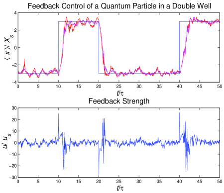
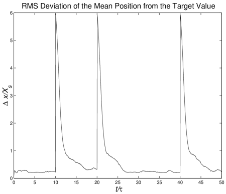
As a particular example we choose and , which puts the two minima at , with a well depth of . Since we set , this puts the problem deep in the quantum regime, since the potential varies considerably over the phase space area . Because of this, the density (Wigner function) for the particle is forced to be broad on the scale of the occupiable phase space, which is a key limiting factor in the problem. We choose , which gives a thermal heating rate . Due to the thermal heating, feedback control is essential to maintain a desired behavior. In implementing the sub-optimal estimation and control strategy described above, we have the choice of measurement strength and feedback strength . We find that it is possible to obtain a fairly effective control with a choice of and . A resulting trajectory for the system, given a target position that switches between the well minima is shown in figure 1, along with the strength of the linear force applied as a result of the control strategy. To evaluate the efficacy of the control, we also plot the RMS deviation of the average position from the target position, and plot this in Figure 2. We see from this that the system achieves the target position within an average error of . When the target is switched, the system relaxes to the desired value with a time constant of .
While this strategy is fairly effective, it is limited by specifically quantum effects. In order to maintain a Gaussian state in the presence of the non-linear potential the combined effect of the thermal noise and measurement must be sufficiently strong, and this results in unwanted heating which must be countered by the feedback. While this is a limitation of the Gaussian estimator, there is still a more fundamental limitation. In the presence of noise, the measurement must be sufficiently strong in order to obtain sufficient information about the system to control it. In this case we found we needed a measurement strength three times that of the noise, resulting in the corresponding heating. Naturally, these quantum limiting features are ultimately due to the size of ; as decreases, the measurement induced heating rate, as well as the rate at which the Wigner function deforms from Gaussian, is reduced. It is to be expected that with the use of more sophisticated estimation techniques, and more subtle quantum control strategies, the simple method we have outlined here can be beaten, possibly significantly, and the development of such techniques constitutes a central problem for future work in quantum feedback control.
VII Conclusion
In this paper we have argued that it is useful to consider quantum feedback control in the light of methods developed in classical control theory. In order to do this it is important to understand the relationship between the two theories. We began by comparing the formulations of these theories, in order to identify conceptual analogies. We then considered three ways in which the quantum control problem could be formally mapped to the classical problem, and discussed if and when these formulations may be addressed directly with the classical theory.
As an example, we applied the ideas presented here to the control of the position of a single quantum particle in a non-linear potential deep in the quantum regime. In this case we fixed both the measurement observable (system/environment coupling) and the unraveling, and considered the use of sub-optimal estimation and control strategies. While this approach was fairly effective, it is clearly limited by quantum effects.
As experimental techniques improve, and quantum technology becomes increasingly relevant in practical applications, we can anticipate that questions of quantum feedback control will become increasingly important. It is clear that most questions regarding the optimal observables, unravelings, and control strategies required for quantum feedback control problems, and the effectiveness of sub-optimal estimation algorithms, are as yet unanswered, and that this field presents a considerable theoretical challenge for future work.
VIII acknowledgements
SH, KJ and HM would like to thank Tanmoy Bhattacharya, Chris Fuchs and Howard Barnum for helpful discussions. This research was performed in part using the resources located at the Advanced Computing Laboratory of Los Alamos National Laboratory.
REFERENCES
- [1] H. Mabuchi, J. Ye, and H.J. Kimble, Appl. Phys. B, 1095 (1999), Eprint: quant-ph/9805076.
- [2] B.E. King, C.S. Wood, C.J. Myatt, Q.A. Turchette, D. Leibfried, W.M. Itano, C. Monroe, and D.J. Wineland, Phys. Rev. Lett. 81, 1525 (1998), Eprint: quant-ph/9803023.
- [3] M.R. Andrews et al, Science 273, 84 (1996).
- [4] H.M. Wiseman and G.J. Milburn, Phys. Rev. Lett. 70, 548 (1993); Phys. Rev. A 49, 2133 (1994); ibid 49, 5159(E) (1994); ibid 50, 4428(E) (1994).
- [5] M.S. Taubman, H.M. Wiseman, D.E. McClelland, and H.-A. Bachor, J. Opt. Soc. Am. B 12, 1792 (1995); H.M. Wiseman, Phys. Rev. Lett. 81, 3840 (1998), Eprint: quant-ph/9805077.
- [6] J.J. Slosser and G.J. Milburn, Phys. Rev. Lett. 75, 418 (1995); P. Tombesi and D. Vitali, Appl. Phys. B 60, S69 (1995); Phys. Rev. A 51, 4913 (1995); P. Goetsch, P. Tombesi, and D. Vitali, Phys. Rev. A 54, 4519 (1996); D.B. Horoshko and S.Ya. Kilin, Phys. Rev. Lett. 78, 840 (1997).
- [7] J.A. Dunningham, H.M. Wiseman, and D.F. Walls, Phys. Rev. A 55, 1398 (1997); S. Mancini and P. Tombesi, Phys. Rev. A 56, 2466 (1997); S. Mancini, D. Vitali, and P. Tombesi, Phys. Rev. Lett. 80, 688 (1998), Eprint: quant-ph/9802034.
- [8] H.F. Hofman, G. Mahler, and O. Hess, Phys. Rev. A 57, 4877 (1998).
- [9] E. Knill, L. Viola and S. Lloyd, Phys. Rev. Lett. 82, 2417 (1999); L. Viola and S. Lloyd, Phys. Rev. A 58, 2733 (1998).
- [10] H. Rabitz W.S. Warren and M. Dahleh, Science 259, 1581 (1993).
- [11] V.P. Belavkin, Non-demolition measurement and control in quantum dynamical systems, In: Information complexity and control in quantum physics, ed. A. Blaquiere, S. Diner and G. Lochak, (Springer-Verlag, New York, 1987).
- [12] A.C. Doherty and K. Jacobs, Phys. Rev. A 60, 2700 (1999), Eprint: quant-ph/9812004.
- [13] P. Cohadon, A. Heidmann, and M. Pinard, Phys.Rev.Lett. 83 3174 (1999), Eprint: quant-ph/9903094.
- [14] O.L.R. Jacobs, Introduction to Control Theory, (Oxford University Press, Oxford, 1993).
- [15] P.S. Maybeck, Stochastic Models, Estimation and Control, volumes II and III, (Academic Press, New York, 1982).
- [16] P. Whittle, Optimal Control, (John Wiley & Sons, Chichester, 1996).
- [17] A. Bensoussan, Stochastic Control of Partialy Observable Systems, (Cambridge University Press, Cambridge, 1992).
- [18] B.D.O. Anderson and J.B. Moore, Optimal Control: Linear Quadratic Methods, (Prentice-Hall, Englewood Cliffs, New Jersey, 1990).
- [19] K. Zhou, J.C. Doyle, and K. Glover, Robust and Optimal Control, (Prentice Hall, New Jersey, 1996).
- [20] H.J. Carmichael, S. Singh, R. Vyas and P.R. Rice, Phys. Rev. A 39, 1200 (1989); G.C. Hegerfeldt and T.S. Wilser, in Proceedings of the II International Wigner Symposium, Goslar, Germany, July 1991, ed. H.D. Döbner, W. Scherer and F. Schröck (World Scientific, Singapore, 1992); J. Dalibard, Y. Castin and K. Molmer, Phys. Rev. Lett. 68, 580 (1992).
- [21] C.W. Gardiner, A.S. Parkins and P. Zoller, Phys. Rev. A 46, 4363 (1992).
- [22] H.J. Carmichael, An Open Systems Approach to Quantum Optics, Lecture Notes in Physics m18, (Springer-Verlag, Berlin, 1993).
- [23] H.M. Wiseman and G.J. Milburn, Phys. Rev. A 47, 642 (1993).
- [24] M.D. Srinivas and E.B. Davies, Optica Acta 28, 981 (1981); N. Gisin, Phys. Rev. Lett. 52, 1657 (1984); L. Diosi, Phys. Lett. A 114, 451 (1986).
- [25] H.M. Wiseman, Phys. Rev. A 75, 4587 (1995).
- [26] V.P. Belavkin, Automat. Remote Control, 44 178 (1983).
- [27] V.P. Belavkin, Rep. Math. Phys. 43, 405 (1999).
- [28] C.A. Fuchs and C.M. Caves, Phys. Rev. Lett. 73, 3047 (1994).
- [29] J. Botina and H. Rabitz, Phys. Rev. A 55 1634 (1997).
- [30] T.A. Brun, I.C. Percival, and R. Schack, J. Phys A: Math. Gen. 29 2077 (1996); M. Patriarca C. Presilla, R. Onofrio, J. Phys A: Math. Gen. 30, 7385 (1997); T. Bhattacharya, S. Habib, and K. Jacobs, Continuous Quantum Measurement and the Emergence of Classical Chaos, Eprint: quant-ph/9906092.
- [31] A.C. Doherty, S.M. Tan, A.S. Parkins, and D.F. Walls, Phys. Rev. A 60 2380 (1999), Eprint: quant-ph/9903030.
- [32] K. Jacobs and P.L. Knight, Phys. Rev. A 57, 2301 (1998), Eprint: quant-ph/9801042.
- [33] G.M. Huang, T.J. Tarn, and J.W. Clark, J. Math. Phys. 24, 2608 (1983); V. Ramakrishna, M.V. Salapaka, M. Dahleh, H. Rabitz, and A. Peirce, Phys. Rev. A 51, 960 (1995).
- [34] S. Lloyd, Phys. Rev. Lett 75, 346 (1995); D. Deutsch, A. Barenco, and A. Ekert, Proc. Roy. Soc. A 449, 669 (1995); S. Lloyd, Quantum controllers for quantum systems, Eprint: quant-ph/9703042; S. Lloyd and S.L. Braunstein, Phys. Rev. Lett 82, 1784 (1999, Eprint: quant-ph/9810082.
- [35] J.J. Halliwell and A. Zoupas, PRD 52, 7294 (1995).