Path integrals and symmetry breaking for optimal control theory

Abstract

This paper considers linear-quadratic control of a non-linear dynamical system subject to arbitrary cost. I show that for this class of stochastic control problems the non-linear Hamilton-Jacobi-Bellman equation can be transformed into a linear equation. The transformation is similar to the transformation used to relate the classical Hamilton-Jacobi equation to the Schrödinger equation. As a result of the linearity, the usual backward computation can be replaced by a forward diffusion process, that can be computed by stochastic integration or by the evaluation of a path integral. It is shown, how in the deterministic limit the PMP formalism is recovered. The significance of the path integral approach is that it forms the basis for a number of efficient computational methods, such as MC sampling, the Laplace approximation and the variational approximation. We show the effectiveness of the first two methods in number of examples. Examples are given that show the qualitative difference between stochastic and deterministic control and the occurrence of symmetry breaking as a function of the noise.

1 Introduction

The problem of optimal control of non-linear systems in the presence of noise occurs in many areas of science and engineering. Examples are the control of movement in biological systems, robotics, and financial investment policies.

In the absence of noise, the optimal control problem can be solved in two ways: using the Pontryagin Minimum Principle (PMP) [1] which is a pair of ordinary differential equations that are similar to the Hamilton equations of motion or the Hamilton-Jacobi-Bellman (HJB) equation which is a partial differential equation [2].

In the presence of Wiener noise, the PMP formalism can be generalized and yields a set of coupled stochastic differential equations, but they become difficult to solve due to the boundary conditions at initial and final time (see however [3]). In contrast, the inclusion of noise in the HJB framework is mathematically quite straight-forward. However, the numerical solution of either the deterministic or stochastic HJB equation is in general difficult due to the curse of dimensionality. Therefore, one is interested in efficient methods for solving the HJB equation. The class of problems considered below allows for such efficient methods.

In section 3.1, we consider the control of an arbitrary non-linear dynamical system with arbitrary cost, but with the restriction, that the control acts linearly on the dynamics and the cost of the control is quadratic. For this class of problems, the non-linear Hamilton-Jacobi-Bellman equation can be transformed into a linear equation by a log transformation of the cost-to-go. The transformation stems back to the early days of quantum mechanics and was first used by Schrödinger to relate the Hamilton-Jacobi formalism to the Schrödinger equation. See section 7 for a further discussion on this point. The log transform was first used in the context of control theory by [4] (see also [5]).

Due to the linear description, the usual backward integration in time of the HJB equation can be replaced by computing expectation values under a forward diffusion process. This is treated in section 3.2. The computation of the expectation value requires a stochastic integration over trajectories that can be described by a path integral (section 3.3). This is an integral over all trajectories starting at $x,t$, weighted by $\exp(-S/\nu)$, where $S$ is the cost of the path (also know as the Action) and $\nu$ is the size of the noise. It has the characteristic form of a partition sum and one should therefore expect that for different values of the noise $\nu$ the control is qualitatively different, and that symmetry breaking occurs below a critical value of $\nu$.

In general, control problems may have several solutions, corresponding to the different local minima of $S$. The case is illustrated in fig. 1. A spider wants to go home, by either crossing a bridge or by going around the lake. In the absence of noise, the route over the bridge is optimal since it is shorter. However, the spider just came out of the local bar, where it had been drinking heavily with its friends. He is not quite sure about the outcome of its actions: any of its movements may be accompanied by a random sway to the left or right. Since the bridge is rather narrow, and spiders don’t like swimming, the optimal trajectory is now to walk around the lake.

Figure 1: The drunken spider. In the absence of noise (alcohol in this case), the optimal trajectory for the spider is to walk over the bridge. When noise is present, there is a significant probability to fall off the bridge, incurring a large cost. Thus, the optimal noisy control is to walk around the lake.

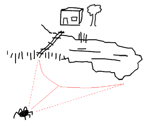
Thus, we see that the optimal control in the presence of noise can be quantitatively different from the deterministic control.

In addition to which path to chose, the spider also has the problem when to make that decision. Far away from the lake, he is in no position to chose for the bridge or the detour, as he is still uncertain of where his random swaying may bring him. In other words, why would he spend control effort now to move left or right when there is a 50 % change that he may wander there by chance? He decides to delay his choice until he is closer to the lake. The question is, when should he make his decision to move left or right?

It is in these multi-modal examples, that the difference between deterministic and stochastic control becomes most apparent. They are not only of concern to spiders, but occur quite general in obstacle avoidance for autonomous systems, differential games, and predator-prey scenarios. Current efficient approaches to control are essentially restricted to unimodal situations and therefore cannot address these issues. The aim of the present paper is to introduce a class of multimodal control problems that can be efficiently solved using path integral methods.

The path integral formulation is well-known in statistical physics and quantum mechanics, and several methods exist to compute them approximately. The Laplace approximation approximates the integral by the path of minimal $S$ and is treated in section 4. This approximation is exact in the limit of $\nu\rightarrow 0$, and the deterministic control law is recovered. The formalism is illustrated for the linear quadratic case in section 4.2. Further refinements to the Laplace approximation can be made by considering the quadratic fluctuations around the deterministic solution (also know as the semi-classical approximation), but I believe that this correction has a small effect on the control (it does strongly affect the value of $J$ but not its gradient). The semi-classical approximation is not treated in this paper.

As is shown in section 4.3, in the Laplace approximation the optimal stochastic control becomes a mixture of deterministic control strategies, weighted by $\exp(-S/\nu)$ and can be computed efficiently, The path integral displays a symmetry breaking at a critical value of $\nu$: For large $\nu$, the optimal control is the average of the deterministic controls. For small $\nu$, one of the deterministic controls is chosen. In section 6.1.2 we give the example of the delayed choice problem that displays such symmetry breaking as a function of the time to reach the target.

In general, the Laplace approximation may not be sufficiently accurate. Possibly the simplest alternative is Monte Carlo (MC) sampling. The naive sampling procedure proposed by the theory is presented in section 5.1, but is shown to be rather inefficient in the double slit example in section 6.1. It is not difficult to devise more efficient samplers. In section 5.2, we propose an importance sampling scheme, where the sampling distribution is a (mixture of) diffusion processes with drift given by the Laplace deterministic trajectories. The importance sampling method is compared with the exact results for the double slit problem in section 6.1.1. In section 6.2, we compute the optimal control for the drunken spider for low noise using the Laplace approximation and for high noise using MC importance sampling.

We begin our story with a brief derivation of the HJB equation for stochastic optimal control, which is treated in depth in many good textbooks (see for instance [6, 5, 3]).

2 Stochastic optimal control

Consider the stochastic differential equation

$$dx=b(x(t),u(t),t)dt+d\xi.$$ (1)

$x,b,d\xi$ and $dx$ are $n$-dimensional vectors and $u$ is an $m$-dimensional vector of controls. $d\xi$ is a Wiener processes with $\left<d\xi_{k}d\xi_{l}\right>=\nu_{kl}(x,u,t)dt$. The initial state of $x$ is fixed: $x(t_{i})=x_{i}$ and the state at final time $t_{f}$ is free. The problem is to find a control trajectory $u(t),t_{i}<t<t_{f}$, such that

$$C(x_{i},t_{i},u(\cdot))=\left<\phi(x(t_{f}))+\int_{t_{i}}^{t_{f}}dtf_{0}(x(t),u(t),t)\right>_{x_{i}}$$ (2)

is minimal. The subscript $x_{i}$ on the expectation value is to remind us that the expectation is over all stochastic trajectories that start in $x_{i}$.

The standard construction of the solution for this problem is to set up a partial differential equation that is to be solved for all times in the interval $t_{i}$ to $t_{f}$ and for all $x$. For this purpose, we define the optimal cost-to-go function from any intermediate time $t$ and state $x$:

$$J(x,t) = \min_{u(t\rightarrow t_{f})}C(x,t,u(t\rightarrow t_{f}))$$ (3)

where $u(t\rightarrow t_{f})$ denotes the sequence of controls $u(\cdot)$ on the time interval $[t,t_{f}]$. For any intermediate time $t^{\prime},t<t^{\prime}<t_{f}$ we can write a recursive formula for $J$ in the following way:

$$J(x,t) = \min_{u(t\rightarrow t_{f})}\left<\phi(x(t_{f}))+\int_{t}^{t^{\prime}}dtf_{0}(x(t),u(t),t)+\int_{t^{\prime}}^{t_{f}}dtf_{0}(x(t),u(t),t)\right>_{x}$$ (4)

$$= \min_{u(t\rightarrow t^{\prime})}\left<\int_{t}^{t^{\prime}}dtf_{0}(x(t),u(t),t)+\min_{u(t^{\prime}\rightarrow t_{f})}\left<\phi(x(t_{f}))+\int_{t^{\prime}}^{t_{f}}dtf_{0}(x(t),u(t),t)\right>_{x(t^{\prime})}\right>_{x}$$

$$= \min_{u(t\rightarrow t^{\prime})}\left<\int_{t}^{t^{\prime}}dtf_{0}(x(t),u(t),t)+J(x(t^{\prime}),t^{\prime})\right>_{x}$$

The first line is just the definition of $J$. In the second line, we split the minimization over two intervals. These are not independent, because the second minimization is conditioned on the starting value $x(t^{\prime})$, which depends on the outcome of the first minimization. The last line uses again the definition of $J$.

Setting $t^{\prime}=t+dt$ we can Taylor expand $J(x(t^{\prime}),t^{\prime})$ around $t$. This expansion takes place within the expectation value and need to be performed to first order in $dt$ and second order in $dx$, since $\left<dx^{2}\right>={\cal O}(dt)$. This is the standard Itô calculus argument. Thus,

$$\left<J(x(t+dt),t+dt)\right>_{x} = \left<J(x,t)+\partial_{t}J(x,t)dt+(\partial_{x}J(x,t))^{T}dx+\frac{1}{2}\mathrm{Tr}\left(\partial_{x}^{2}J(x,t)dx^{2}\right)\right>$$

$$= J(x,t)+\partial_{t}J(x,t)dt+(\partial_{x}J(x,t))^{T}b(x,u,t)dt+\frac{1}{2}\mathrm{Tr}\left(\partial_{x}^{2}J(x,t)\nu(x,u,t)\right)dt$$

In this expression, $\partial_{t}$ and $\partial_{x}$ denotes partial differentiation with respect to $t$ and $x$, respectively. Similarly, $\partial^{2}_{x}J$ is the matrix of second derivatives of $J$ and $\mathrm{Tr}(\nu\partial_{x}^{2}J)=\sum_{ij}\nu_{ij}\frac{\partial^{2}J}{\partial x_{i}\partial x_{j}}$. Substituting this into Eq. 4, dividing both sides by $dt$ and taking the limit of $dt\rightarrow 0$ yields

$$-\partial_{t}J(x,t)=\min_{u}\left(f_{0}(x,u,t)+b(x,u,t)^{T}\partial_{x}J(x,t)+\frac{1}{2}\mathrm{Tr}\left(\nu(x,u,t)\partial_{x}^{2}J(x,t)\right)\right),\quad\forall t,x$$ (5)

which is the Stochastic Hamilton-Jacobi-Bellman Equation with boundary condition $J(x,t_{f})=\phi(x)$.

Eq. 5 reduces to the deterministic HJB equation in the limit $\nu\rightarrow 0$. In that case, an alternative approach to solving the control problem is the Pontryagin Maximum principle (PMP), which requires the solution of $2n$ ordinary differential equations. These equations need to be solved with multi-point boundary conditions at both $t_{i}$ and $t_{f}$. Solving $2n$ ordinary differential equations may be more efficient than solving the $n$-dimensional partial differential equation, using shooting methods (see for instance [7]), but may be unstable in some cases.

In the stochastic case, there does not exist a generic alternative to solving the pde (see however [3] for stochastic versions of the PMP approach). Thus, for stochastic control one needs to solve the HJB equation, which suffers from the curse of dimensionality.

A notable exception is when $b$ is linear in $x$ and $u$ and $f_{0}$ is quadratic in $x$ and $u$. This is called the linear-quadratic (LQ) control problem. In that case, it can be shown that the solution for $J(x,t)$ is quadratic in $x$ with time-varying coefficients. These coefficients satisfy coupled ordinary differential (Ricatti) equations that can be solved efficiently [6].

3 A path integral formulation for control

3.1 A linear HJB equation

Consider the special case of Eqs. 1 and 2 where the dynamic is linear in $u$ and the cost is quadratic in $u$:

$$dx = (b(x,t)+Bu)dt+d\xi$$ (6)

$$C(x_{i},t_{i},u(\cdot)) = \left<\phi(x(t_{f}))+\int_{t_{i}}^{t_{f}}dt\left(\frac{1}{2}u(t)^{T}Ru(t)+V(x(t),t)\right)\right>_{x_{i}}$$ (7)

with $B$ an $n\times m$ matrix and $R$ an $m\times m$ matrix. $B$, $R$ and $\nu$ are independent of $x,u,t$. $b$ and $V$ are arbitrary functions of $x$ and $t$ and $\phi$ is an arbitrary function of $x$. In other words, the system to be controlled can be arbitrary complex and subject to arbitrary complex costs. The control instead, is restricted to the simple LQ form.

The stochastic HJB equation 5 becomes

$$-\partial_{t}J = \min_{u}\left(\frac{1}{2}u^{T}Ru+V+(b+Bu)^{T}\partial_{x}J+\frac{1}{2}\mathrm{Tr}\left(\nu\partial_{x}^{2}J\right)\right)$$

Minimization with respect to $u$ yields:

$$u=-R^{-1}B^{T}\partial_{x}J(x,t)$$ (8)

which defines the optimal control $u$ for each $x,t$. The HJB equation becomes

$$-\partial_{t}J = -\frac{1}{2}(\partial_{x}J)^{T}BR^{-1}B^{T}\partial_{x}J+V+b^{T}\partial_{x}J+\frac{1}{2}\mathrm{Tr}\left(\nu\partial_{x}^{2}J\right)$$

This partial differential equation must be solved with boundary condition $J(x,t_{f})=\phi(x)$. Note, that after performing the minimization with respect to to $u$, the HJB equation has become non-linear in $J$.

We can remove the non-linearity and this will turn out to greatly help us to solve the HJB equation. Define $\psi(x,t)$ through $J(x,t)=-\lambda\log\psi(x,t)$, with $\lambda$ a constant to be defined. Then

$$-\frac{1}{2}(\partial_{x}J)^{T}BR^{-1}B^{T}\partial_{x}J+\frac{1}{2}\mathrm{Tr}\left(\nu\partial^{2}_{x}J\right)$$

$$= -\frac{\lambda^{2}}{2\psi^{2}}\sum_{ij}(\partial_{x}\psi)_{i}(BR^{-1}B^{T})_{ij}(\partial_{x}\psi)_{j}+\frac{\lambda}{2\psi^{2}}\sum_{ij}\nu_{ij}(\partial_{x}\psi)_{i}(\partial_{x}\psi)_{j}-\frac{\lambda}{2\psi}\sum_{ij}\nu_{ij}\frac{\partial^{2}\psi}{\partial x_{i}\partial x_{j}}$$

The terms quadratic in $\psi$ vanish if and only if there exists a scalar $\lambda$ such that

$$\nu=\lambda BR^{-1}B^{T}$$ (9)

In other words, the matrices $\nu$ and $BR^{-1}B^{T}$ must be proportional to each other with proportionality constant $\lambda$. In the one dimensional case, such a $\lambda$ always exists, and Eq. 9 is not a restriction. In the higher dimensional case, Eq. 9 restricts the possible choices for the matrices $R$ and $\nu$. To get an intuition for this restriction, consider the case that $u$ and $x$ have the same dimension, $B$ is the identity matrix and both $R$ and $\nu$ are diagonal matrices. Then Eq. 9 states $R\propto\nu^{-1}$. In a direction with low noise, control is expensive ($R_{ii}$ large) and only small control steps are permitted. In the limiting case of no noise, we deduce that $u$ should be set to zero: no control is allowed in noiseless directions. In noisy directions the reverse is true: control is cheap and large control values are permitted. Loosely speaking, Eq. 9 states that noise and control should operate in the same dimensions.

When Eq. 9 holds, the quadratic terms in the HJB equation cancel and the HJB becomes

$$\partial_{t}\psi = \left(\frac{V}{\lambda}-b^{T}\partial_{x}-\frac{1}{2}\mathrm{Tr}(\nu\partial^{2}_{x})\right)\psi$$ (10)

$$= -H\psi$$

with $H$ a linear operator acting on the function $\psi$. Eq. 10 must be solved backwards in time with $\psi(x,t_{f})=\exp(-\phi(x)/\lambda)$. However, the linearity allows us to reverse the direction of computation, replacing it by a diffusion process, as we will explain in the next section.

To simplify the exposure in the subsequent sections, we assume the control dimension $m=n$ and $B$ the unit matrix.

3.2 Forward diffusion

For real functions $\rho$ and $\psi$, define the inner product $\left<\rho|\psi\right>=\int dx\rho(x,t)\psi(x,t)$. Then we can define $H^{\dagger}$, the Hermitian conjugate of the operator $H$, with respect to this inner product as follows.

$$\left<H^{\dagger}\rho|\psi\right> = \left<\rho|H\psi\right>=\int dx\rho(x,t)\left(-\frac{V(x,t)}{\lambda}+b(x,t)\partial_{x}+\frac{1}{2}\sum_{ij}\nu_{ij}\frac{\partial^{2}}{\partial x_{i}\partial x_{j}}\right)\psi(x,t)$$

$$= \int dx\left(-\frac{V(x,t)}{\lambda}\rho(x,t)-\partial_{x}(b(x,t)\rho(x,t))+\frac{1}{2}\sum_{ij}\nu_{ij}\frac{\partial^{2}}{\partial x_{i}\partial x_{j}}\rho(x,t)\right)\psi(x,t)$$

where we have performed integration by parts and assume that $\rho$ vanishes at $|x|\rightarrow\infty$. Thus,

$$H^{\dagger}\rho = -\frac{V(x,t)}{\lambda}\rho(x,t)-\partial_{x}(b(x,t)\rho(x,t))+\frac{1}{2}\sum_{ij}\nu_{ij}\frac{\partial^{2}}{\partial x_{i}\partial x_{j}}\rho(x,t).$$

Let $\rho(y,\tau|x,t)$ be a probability density, initialized at $t,x$, that evolves forward in time according to the diffusion process

$$\partial_{t}\rho=H^{\dagger}\rho$$ (11)

with drift $b(x,t)dt$ and diffusion $d\xi$, and with an extra term due to the potential $V$. Whereas the other two terms conserve probability density, the potential term takes out probability density at a rate $V(x,t)dt/\lambda$. Therefore, the stochastic simulation of Eq. 11 is a diffusion that runs in parallel with the annihilation process:

$$dx = b(x,t)dt+d\xi$$

$$x = x+dx,\quad\mbox{with probability}~{}~{}1-V(x,t)dt/\lambda$$

$$x_{i} = \dagger,\quad\mbox{with probability}~{}~{}V(x,t)dt/\lambda$$ (12)

where $\dagger$ denotes that the particle is taken out of the simulation. Note that when $V=0$ this diffusion process is identical to the original control dynamics Eq. 6 in the absence of control ($u=0$).

Since $\psi$ evolves backwards in time according to $H$ and $\rho$ evolves forwards in time according to $H^{\dagger}$ the inner product $\int dy\rho(y,\tau|x,t)\psi(y,\tau)$ is time invariant (independent of $\tau$). Since $\rho(y,t|x,t)=\delta(y-x)$, it immediately follows that

$$\psi(x,t) = \int dy\rho(y,t_{f}|x,t)\psi(y,t_{f})$$ (13)

We arrive at the important conclusion that $\psi(x,t)$ can be computed either by backward integration using Eq. 10 or by forward integration of a diffusion process given by Eq. 11. The optimal cost-to-go is finally given by

$$J(x,t) = -\lambda\log\int dy\rho(y,t_{f}|x,t)\exp(-\phi(y)/\lambda)$$ (14)

with $\rho(y,t_{f}|x,t)$ given by the stochastic process Eq. 12. The optimal control is given by Eq. 8. See section 4.2 for a simple Gaussian example that illustrate these ideas.

3.3 The path integral formulation

In this section, we will write the diffusion kernel $\rho(y,t_{f}|x,t)$ in Eq. 14 as a path integral. For an infinitesimal time step $\epsilon$, we can write the probability to go from $x$ to $y$ as an integral over all noise realizations. The probability of the Wiener is Gaussian with mean zero and variance $\nu\epsilon$. The particle annihilation destroys probability with rate $V(x,t)\epsilon/\lambda$. Combining annihilation with diffusion, we obtain

$$\rho(y,t+\epsilon|x,t) \propto \exp\left(-\frac{\epsilon}{\lambda}\left[\frac{1}{2}\left(\frac{y-x}{\epsilon}-b(x,t)\right)^{T}R\left(\frac{y-x}{\epsilon}-b(x,t)\right)+V(x,t)\right]\right)$$

where we have used $\nu^{-1}=R/\lambda$.

We can write the transition probability as a product of $n$ infinitesimal transition probabilities:

$$\rho(y,t_{f}|x,t) \propto \int dx_{1}\ldots dx_{n-1}$$

$$\exp\left(-\frac{\epsilon}{\lambda}\sum_{i=0}^{n-1}\left[\frac{1}{2}\left(\frac{x_{i+1}-x_{i}}{\epsilon}-b(x_{i},t_{i})\right)^{T}R\left(\frac{x_{i+1}-x_{i}}{\epsilon}-b(x_{i},t_{i})\right)+V(x_{i},t_{i})\right]\right)$$

In the limit of $\epsilon\rightarrow 0$, the sum in the exponent becomes an integral: $\epsilon\sum_{i=0}^{n-1}\rightarrow\int_{t}^{t_{f}}d\tau$ and thus we can formally write

$$\rho(y,t_{f}|x,t) = \int[dx]_{x}^{y}\exp\left(-\frac{1}{\lambda}S_{\mathrm{path}}(x(t\rightarrow t_{f}))\right)$$ (15)

$$S_{\mathrm{path}}(x(t\rightarrow t_{f})) = \int_{t}^{t_{f}}d\tau\left(\frac{1}{2}\left(\frac{dx(\tau)}{d\tau}-b(x(\tau),\tau)\right)^{T}R\left(\frac{dx(\tau)}{d\tau}-b(x(\tau),\tau)\right)+V(x(\tau),\tau)\right)$$ (16)

with $x(t\rightarrow t_{f})$ a path with $x(\tau=t)=x,x(\tau=t_{f})=y$, $\int[dx]_{x}^{y}$ an integral over paths that start at $x$ and end at $y$.

Substituting Eq. 15 in Eq. 14 we can absorb the integration over $y$ in the path integral and find

$$J(x,t) = -\lambda\log\int[dx]_{x}\exp\left(-\frac{1}{\lambda}S(x(t\rightarrow t_{f}))\right)$$ (17)

where the path integral $\int[dx]_{x}$ is over all trajectories starting at $x$ and

$$S(x(t\rightarrow t_{f})) = \phi(x(t_{f}))+S_{\mathrm{path}}(x(t\rightarrow t_{f}))$$ (18)

is the Action associated with a path.

The path integral Eq. 17 is a log partition sum and therefore can be interpreted as a free energy. The partition sum is not over configurations, but over trajectories. $S(x(t\rightarrow t_{f}))$ plays the role of the energy of a trajectory and $\lambda$ is the temperature. This link between stochastic optimal control and a free energy has two immediate consequences. 1) Phenomena that allow for a free energy description, typically display phase transitions and spontaneous symmetry breaking. What is the meaning of these phenomena for optimal control? 2) Since the path integral appears in other branches of physics, such as statistical mechanics and quantum mechanics, we can borrow approximation methods from those fields to compute the optimal control approximately. First we discuss the small noise limit, where we can use the Laplace approximation to recover the PMP formalism for deterministic control. Also, the path integral shows us how we can obtain a number of approximate methods: 1) one can combine multiple deterministic trajectories to compute the optimal stochastic control 2) one can use a variational method, replacing the intractable sum by a tractable sum over a variational distribution and 3) one can design improvements to the naive MC sampling.

4 The Laplace approximation

4.1 The Laplace approximation

When $\lambda$ is small (i.e. $\nu$ is small), we can expand an arbitrary path $\tilde{x}(\tau)$ around the classical path:

$$\tilde{x}(\tau)=x(\tau)+\delta(\tau),\quad t<\tau<t_{f}$$

where $x(\tau)$ is the classical path that we need to determine, and $\delta(\tau)$ is an independent fluctuation of the path at time $\tau$. Fluctuations are also allowed at $\tau=t$ and $\tau=t_{f}$. The Action Eq. 18 can be expanded to first order in $\delta(\tau)$ as

$$S(\tilde{x}(t\rightarrow t_{f})) = S(x(t\rightarrow t_{f}))+\delta_{i}(t_{f})\partial_{i}\phi(x(t_{f}))$$ (19)

$$+ \int_{t}^{t_{f}}d\tau\left((\dot{x}(\tau)-b(x,\tau))_{i}R_{ij}\left(\frac{d}{d\tau}\delta_{j}(\tau)-\delta_{k}(\tau)\partial_{k}b_{j}(x,\tau)\right)+\delta_{i}(\tau)\partial_{i}V(x(\tau),\tau)\right)$$

$$= S(x(t\rightarrow t_{f}))+\delta_{i}(t_{f})\left(\partial_{i}\phi(x(t_{f}))+p_{j}(t_{f})\right)-p_{j}(t)\delta_{j}(t)$$

$$- \int_{t}^{t_{f}}d\tau\delta_{k}(\tau)\left(\frac{d}{d\tau}p_{k}(\tau)+p_{j}(\tau)\partial_{k}b_{j}(x,\tau)-\partial_{k}V(x(\tau),\tau)\right)$$

where $\partial_{k}$ means partial differentiation with respect to $x_{k}$, repeated indices are summed over and $p$ is defined as

$$p_{k}(t)=(\dot{x}(t)-b(x,t))_{j}R_{jk}$$ (20)

The term proportional to $\delta_{k}(\tau)$ under the integral must be zero and defines an ODE for the classical trajectory:

$$\frac{d}{dt}p_{k}(t)+\frac{\partial}{\partial x_{k}}\left(p_{j}(t)b_{j}(x,t)-V(x,t)\right)=0$$ (21)

Eq. 20 can be seen as a definition of $p$, but also as a dynamical equation for $x$ that must be solved together with the dynamical equation for $p$, Eq. 21. These equations must be solved with boundary conditions. The boundary condition for $x$ is given at initial time and the term proportional to $\delta_{i}(t_{f})$ defines the boundary condition for $p(t)$ at $t=t_{f}$:

$$x_{i}(t)=x,\qquad p_{j}(t_{f})=-\frac{\partial\phi(x(t_{f}))}{\partial x_{j}}$$ (22)

Define the Hamiltonian,

$$H(x,p,t)=\frac{1}{2}p^{T}R^{-1}p+p^{T}b(x,t)-V(x,t)$$ (23)

Then, Eqs. 20 and 21 can be written as

$$\frac{dx}{dt}=\frac{\partial H(x,p,t)}{\partial p},\qquad\frac{dp}{dt}=-\frac{\partial H(x,p,t)}{\partial x}$$ (24)

The Hamiltonian system Eqs. 24 with the mixed boundary conditions Eqs. 22 are the well-known ordinary differential equations of the Pontryagin Maximum Principle.

In the Laplace approximation, the path integral Eq. 17 is replaced by the classical trajectory only. Thus,

$$J(t,x)\approx S(x(t\rightarrow t_{f}))$$

since fluctuations at initial time are zero: $\delta_{i}(t)=0$. The optimal control is given by

$$u=-R^{-1}\partial_{x}J\approx-R^{-1}\frac{\delta S(x(t\rightarrow t_{f}))}{\delta x(t)}=R^{-1}p(t)=\dot{x}(t)-b(x(t),t)$$ (25)

where we have used $\frac{\delta S(x(t\rightarrow t_{f}))}{\delta x(t)}=-p(t)$ from Eq. 19. The intuition of the Laplace approximation is that one needs to solve the deterministic equations for the whole interval $[t,t_{f}]$, starting at the current place $x$. In particular, the end boundary condition (the location of the target) will affect the location of the optimal path for all $[t\rightarrow t_{f}]$. The control is then given by the value of the pseudo-gradient $\dot{x}(t)-b(x(t),t)$ on this trajectory.

Note the minus sign in front of $V$ in Eq. 23, which has the opposite sign from a normal classical mechanical system. The term $\frac{1}{2}p^{T}R^{-1}p$ can be interpreted as the kinetic energy of the system. Thus, the ’energy’ $H$ is not the sum, but the difference of kinetic and potential energy. When $H$ does not explicitly depend on time ($b(x,t)=b(x)$ and $V(x,t)=V(x)$), $H$ is conserved under the deterministic control dynamics:

$$\frac{dH}{dt}=\frac{\partial H}{\partial x}\frac{dx}{dt}+\frac{\partial H}{\partial p}\frac{dp}{dt}=0$$

because of Eqs. 24. To understand this behavior, consider $b=0$. Then along the trajectory:

$$\frac{1}{2}u^{T}Ru=V(x)+H$$

with $H$ independent of time. This relation states that the optimal trajectory is such that much control is spent in areas of large cost and little control is spent in areas of low cost.

Note, that the optimal control is independent of the noise $\nu$ as we expect from the Laplace approximation. Numerically, we can compute the classical trajectory by discretizing $x_{\mathrm{cl}}(\tau)=x_{1},\ldots,x_{n}$ and minimizing $S(x_{\mathrm{cl}})=S(x_{1},\ldots,x_{n})$ using a standard minimization method.

4.2 The linear quadratic case

To build a bit of intuition for the diffusion process, the path integral and Laplace approximation, we consider in this section some simple one-dimensional linear quadratic examples.

First consider the simplest case of free diffusion:

$$V(x,t)=0,\quad b(x,t)=0,\quad\phi(x)=\frac{1}{2}\alpha x^{2}\quad$$

In this case, the forward diffusion described by Eq. 11 and 12 can be solved in closed form and is given by a Gaussian with variance $\sigma^{2}=\nu(t_{f}-t)$:

$$\rho(y,t_{f}|x,t)=\frac{1}{\sqrt{2\pi}\sigma}\exp\left(-\frac{(y-x)^{2}}{2\sigma^{2}}\right)$$ (26)

Since the end cost is quadratic, the optimal cost-to-go Eq. 14 can be computed exactly as well. The result is

$$J(x,t) = \nu R\log\left(\frac{\sigma}{\sigma_{1}}\right)+\frac{1}{2}\frac{\sigma_{1}^{2}}{\sigma^{2}}\alpha x^{2}$$ (27)

with $1/\sigma_{1}^{2}=1/\sigma^{2}+\alpha/\nu R$. The optimal control is computed from Eq. 8:

$$u=-R^{-1}\partial_{x}J=-R^{-1}\frac{\sigma_{1}^{2}}{\sigma^{2}}\alpha x=-\frac{\alpha x}{R+\alpha(t_{f}-t)}$$

We see that the control attracts $x$ to the origin with a force that increases with $t$ getting closer to $t_{f}$. Note, that the optimal control is independent of the noise $\nu$. This is a general property of LQ control.

As an extension, we now add a quadratic potential to the above problem: $V(x)=\frac{1}{2}\mu x^{2}$. We now compute the optimal control in the Laplace approximation. The Hamiltonian is given by Eq. 23

$$H(x,p)=\frac{1}{2}R^{-1}p^{2}-\frac{1}{2}\mu x^{2}$$

and the equations of motion and boundary conditions are given by Eqs. 24 and 22:

$$\dot{x} = p/R\qquad\dot{p}=\mu x$$

$$x(t) = x\qquad p(t_{f})=-\alpha x(t_{f})$$

We can write this as the second order system in terms of $x$ only:

$$\ddot{x}=\mu x/R,\qquad x(t)=x\qquad\dot{x}(t_{f})=-\alpha x(t_{f})/R$$

The solution for $t<\tau<t_{f}$ is

$$x(\tau)=Ae^{\sqrt{\mu/R}(\tau-t)}+Be^{-\sqrt{\mu/R}(\tau-t)}$$

The boundary conditions become $A+B=x$ and $A\gamma(\sqrt{\mu/R}+\alpha/R)=B/\gamma(\sqrt{\mu/R}-\alpha/R)$, $\gamma=e^{\sqrt{\mu/R}(t_{f}-t)}$ from which we can solve $A$ and $B$. The classical Action Eq. 18 is computed by substituting the solution for $x$ :

$$S(x(t\rightarrow t_{f})) = \frac{1}{2}\alpha x(t_{f})^{2}+\frac{1}{2}\int_{t}^{t_{f}}d\tau(R\dot{x}^{2}(\tau)+\mu x^{2}(\tau))=\frac{1}{2}\sqrt{\mu R}x^{2}\frac{\gamma^{2}-\frac{\sqrt{\mu R}-\alpha}{\sqrt{\mu R}+\alpha}}{\gamma^{2}+\frac{\sqrt{\mu R}-\alpha}{\sqrt{\mu R}+\alpha}}$$

which is equal to the cost-to-go in the Laplace approximation. The optimal control is minus the gradient of the cost-to-go. Note, that the classical trajectory as well as the minimal action only depends on the initial condition $x$ and the time-to-go $t_{f}-t$. For pure diffusion ($\mu\rightarrow 0$) the classical Action reduces to

$$S(x(t\rightarrow t_{f}))=\frac{1}{2}\frac{\alpha Rx^{2}}{R+\alpha(t_{f}-t)}$$

which is identical to the exact expression Eq. 27 except for the volume factor (which does not affect the control, since it does not depend on $x$).

4.3 The multi-modal Laplace approximation

The Action $S$ in Eq. 17 may have more than one local minimum. This is typical for control problems, where ”many roads lead to Rome”. Let $x_{\alpha}(t\rightarrow t_{f}),\alpha=1,\ldots$ denote the different optimal deterministic trajectories that we compute by minimizing the Action:

$$x_{\alpha}(t\rightarrow t_{f})=\mathrm{argmin}_{x(t\rightarrow t_{f})}S(x(t\rightarrow t_{f})),\quad\alpha=1,\ldots$$

These trajectories all start at the same value $x$. In our drunken spider example, there are two trajectories: one is over the bridge and the other is around the lake. Then, in the Laplace approximation the path integral Eq. 17 is approximated by these local minima contributions only:

$$J(x,t) \approx -\lambda\log\sum_{\alpha}\exp(-S(x_{\alpha}(t\rightarrow t_{f})/\lambda)$$ (28)

The Laplace approximation ignores all fluctuations around the mode. Although these fluctuations can be quite big, their $x$ dependence is typically quite weak and must come from beyond Gaussian corrections. This can be seen from the pure LQ case when the Gaussian fluctuation term in Eq. 27 is independent of $x$. In the LQ case, the Laplace approximation for the control (not for the cost-to-go) coincides with the exact solution. Therefore, for unimodal problems ($S$ has only one minimum) one can often safely ignore the contribution of fluctuations to the control. However, for multi-modal problems these fluctuation terms may have a strong $\alpha$ dependence (they have in the spider problem) and therefore play an important role when weighting the different contributions in Eq. 28.

The optimal control becomes a soft-max of deterministic strategies

$$u(x,t) = -R^{-1}\sum_{\alpha}w_{\alpha}\partial_{x}S(x_{\alpha}(t\rightarrow t_{f})$$

$$w_{\alpha} = \frac{e^{-S(x_{\alpha}(t\rightarrow t_{f})/\lambda}}{\sum_{\beta}e^{-S(x_{\beta}(t\rightarrow t_{f})/\lambda}}$$

where $\nu$ plays the role of the temperature.

5 MC sampling

A natural method for computing the optimal control is by stochastic sampling. However, as is often the case with MC sampling, a naive sampler such as the one based directly on Eqs. 12 may be very inefficient. In this section, we show how this naive sampler works and how it can be improved using importance sampling.

5.1 Naive MC sampling

The stochastic evaluation of Eq. 13 consists of running $N$ times the diffusion process Eq. 12 from $t$ to $t_{f}$ initialized each time at $x(t)=x$. Denote these $N$ trajectories by $x_{i}(t\rightarrow t_{f}),i=1,\ldots,N$. Then, $\psi(x,t)$ is estimated by

$$\hat{\psi}(x,t)=\sum_{i\in\mathrm{alive}}w_{i},\qquad w_{i}=\frac{1}{N}\exp(-\phi(x_{i}(t_{f}))/\lambda)$$ (29)

where ’alive’ denotes the subset of trajectories that do not get killed along the way by the $\dagger$ operation. Note that, although the sum is typically over less than $N$ trajectories, the normalization $1/N$ includes all trajectories in order to take the annihilation process properly into account.

The computation of $u$ requires the gradient of $\psi(x,t)$ instead of $\psi$ itself. First note, that when we vary the initial point of a path $x(t\rightarrow t_{f})$ from Eq. 19 and 20 we obtain

$$\frac{\delta S(x(t\rightarrow t_{f}))}{\delta x(t)}=(\dot{x}(t)-b(x,t))R$$

Thus combining Eq. 8 and Eq. 17, we obtain

$$u=\frac{1}{\psi(x,t)}\int[dx]_{x}(\dot{x}(t)-b(x,t))\exp(-S/\lambda)$$

Note, that we can sample $u$ by the same batch of (naive) trajectories. For each trajectory, the quantity $\dot{x}(t)-b(x,t)$ is proportional to the realisation of the noise in the initial time $t$: $\dot{x}(t)-b(x,t)=d\xi_{i}(t)/dt$. Therefore,

$$\hat{u}dt = \frac{1}{\hat{\psi}(x,t)}\sum_{i\in\mathrm{alive}}^{N}w_{i}d\xi_{i}(t)$$ (30)

with $w_{i}$ given by Eq. 29. This expression has a particular intuitive form. The optimal control at time $t$ is obtained by averaging the initial noise directions of the trajectories $d\xi_{i}(t)$, weighted by their success $w_{i}$ at the final time $t_{f}$.

5.2 Importance sampling

The sampling procedure as described by Eqs. 12 and 29 gives an unbiased estimate of $\psi(x,t)$ but can be quite inefficient. The problem is is well known, and one of the simplest procedures for improving the sampling is by importance sampling. For path integrals this works as follows. We replace the diffusion process that yields $\rho(y,t_{f}|x,t)$ with Action $S_{\mathrm{path}}$ (Eqs. 15 and 16) by another diffusion process, that will yield $\rho^{\prime}(y,t_{f}|x,t)$ with corresponding Action $S^{\prime}_{\mathrm{path}}$ . Then,

$$\psi(x,t) = \int[dx]_{x}\exp\left(-S_{\mathrm{path}}/\lambda\right)\exp\left(-\phi/\lambda\right)$$

$$= \int[dx]_{x}\exp\left(-S^{\prime}_{\mathrm{path}}/\lambda\right)\exp\left(-(\phi+S_{\mathrm{path}}-S^{\prime}_{\mathrm{path}})/\lambda\right)$$

The idea is to chose the diffusion process $\rho^{\prime}$ such as to make the sampling of the path integral as efficient as possible.

A suggestion that comes to mind immediately is to use the Laplace approximation to compute a deterministic control trajectory $x^{*}(t\rightarrow t_{f})$. From this, compute its derivative $\dot{x}^{*}(t\rightarrow t_{f})$ and define a stochastic process to sample $\rho^{\prime}$ according to

$$dx = \dot{x}^{*}(t)dt+d\xi$$

$$x = x+dx,\quad\mbox{with probability}~{}~{}1-V(x,t)dt/\lambda$$

$$x_{i} = \dagger,\quad\mbox{with probability}~{}~{}V(x,t)dt/\lambda$$ (31)

The Action $S^{\prime}_{\mathrm{path}}$ for the Laplace-guided diffusion is given by Eq. 16 with $b(x(\tau),\tau)=x^{*}(\tau),t<\tau<t_{f}$.

The estimators for $\psi$ and $u$ are given again by Eqs. 29 and 30, with the difference that

$$w_{i} = \frac{1}{N}\exp\left(-\left(\phi(x_{i}(t_{f}))+S_{\mathrm{path}}(x_{i}(t\rightarrow t_{f}))-S^{\prime}_{\mathrm{path}}(x_{i}(t\rightarrow t_{f}))\right)/\lambda\right)$$ (32)

and $x_{i}(t\rightarrow t_{f})$ is a trajectory from the sampling process Eq. 31 instead of Eq. 12. We will illustrate the effectiveness of this approach in section 6.1.

6 Numerical examples

In this section, we introduce some simple one-dimensional examples to illustrate the methods introduced in this paper. The first example is a double slit, and is sufficiently simple that we can compute the optimal control by forward diffusion in closed form. We use this example to compare the Monte Carlo and Laplace approximations to the exact result. Using the double slit example, we show how the optimal cost-to-go undergoes symmetry breaking as a function of the noise and/or some other characteristics of the problem (in this case the time-to-go). When the targets are still far in the future, the optimal control is to ’steer for the middle’ and delay the choice to a later time.

The second example is similar to the first, except that the slit is now of finite thickness, allowing the particle to get lost in one of the holes. When one hole is narrow and the other wide, this illustrates the drunken spider problem. We use both the Laplace approximation and the the Monte Carlo importance sampling to compute the optimal control strategy, for different noise levels.

6.1 The double slit

Consider a stochastic particle that moves with constant velocity from $t$ to $t_{f}$ in the horizontal direction and where there is deflecting noise in the $x$ direction:

$$dx = udt+d\xi$$

The cost is given by Eq. 7 with $\phi(x)=\frac{1}{2}x^{2}$ and $V(x,t_{1})$ implements a slit at an intermediate time $t_{1}$, $t<t_{1}<t_{f}$:

$$V(x,t_{1}) = 0,\quad a<x<b,\quad c<x<d$$

$$= \infty,\quad\mathrm{else}$$

The problem is illustrated in Fig. 2a where the constant motion is in the $t$ direction and the noise and control is in the $x$ direction perpendicular to it.

Eq. 9 becomes $\lambda=\nu R$ and the linear HJB becomes:

$$\partial_{t}\psi=\left(\frac{V}{\lambda}-\frac{\nu}{2}\partial_{x}^{2}\right)\psi$$

which we must solve with end condition $\psi(x,t_{f})=e^{-\phi(x)/\lambda}$.

Solving this equation by means of the forward computation using Eq. 13 can be done in closed form. First consider the easiest case for times $t>t_{1}$ where we do not have to consider the slits. This is the case we have considered before in section 4.2 and the solution is given by Eq. 27 with $\alpha=1$.

Secondly, consider $t<t_{1}$. $\rho(y,t_{f}|x,t)$ can be written as a diffusion from $t$ to $t_{1}$, times a diffusion from $t_{1}$ to $t_{f}$ integrating over all $x$ in the slits. Substitution in Eq. 13 we obtain

$$\psi(x,t) = \int dy\left(\int_{a}^{b}+\int_{c}^{d}\right)dx_{1}\exp(-y^{2}/2\lambda)\rho(y,t_{f}|x_{1},t_{1})\rho(x_{1},t_{1}|x,t)$$

$\rho(y,t_{f}|x_{1},t_{1})$ is Gaussian and given by Eq. 26. Therefore, we can perform the integration over $y$ in closed form. We are left with an integral over $x_{1}$ that can be expressed in terms of Error functions. The result is

$$J(x,t) = \nu R\log\left(\frac{\sigma}{\sigma_{1}}\right)+\frac{1}{2}\frac{\sigma_{1}^{2}}{\sigma^{2}}x^{2}-\nu R\log\frac{1}{2}\left(F(b,x)-F(a,x)+F(d,x)-F(c,x)\right)$$ (33)

with $F(x_{0},x)=\mbox{Erf}\left(\sqrt{\frac{A}{2\nu}}(x_{0}-\frac{B(x)}{A})\right)$, $A=\frac{1}{t_{1}-t}+\frac{1}{R+t_{f}-t_{1}}$ and $B(x)=\frac{x}{t_{1}-t}$. Eqs. 27 and 33 together provide the solution for the control problem in terms of $J$ and we can compute the optimal control from Eq. 8.

A numerical example for the solution for $J(x,t)$ is shown in fig. 2b. The two parts of the solution (compare $t=0.99$ and $t=1.01$) are smooth at $t=t_{1}$ for $x$ in the slits, but discontinuous at $t=t_{1}$ outside the slits. For $t=0$, the cost-to-go $J$ is higher around the right slit than around the left slit, because the right slit is further removed from the optimal target $x=0$ and thus requires more control $u$ and/or its expected target cost $\phi$ is higher.

(a) The double slit

(b) Cost-to-go $J(x,t)$

Figure 2: (a) The particle moves horizontally with constant velocity from $t=0$ to $t_{f}=2$ and is deflected up or down by noise and control. The end cost $\phi(x)=x^{2}/2$. A double slit is placed at $t_{1}=1$ with openings at $-6<x<-4$ and $6<x<8$. Also shown are two example trajectories under optimal control. (b) $J(x,t)$ as a function of $x$ for $t=0,0.99,1.01,2$ as computed from Eq. 27 and 33. $R=0.1,\nu=1,dt=0.02$.

6.1.1 MC sampling

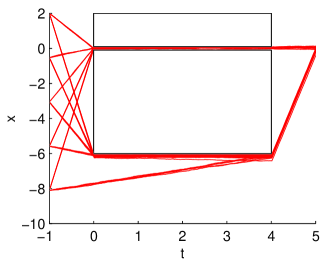
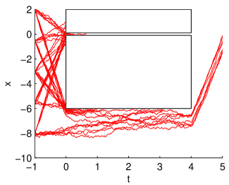
We assess the quality of the naive MC sampling scheme, as given by Eqs. 12 and 29 in fig. 3, where we compare $J(x,0)$ as given by Eq. 33 with the MC estimate Eq. 29.

(a) Sample trajectories

(b) MC sampling estimate of $J(x,0)$

Figure 3: Monte Carlo sampling of $J(x,t=0)$ with $\psi$ from Eq. 12 for the double slit problem. The parameters are as in fig. 2. (a) Sample of trajectories that start at $x$ to estimate $J(x,t)$. Only trajectories that pass through a slit contribute to the estimate. (b) MC estimate of $J(x,t)=0$ with $N=100000$ trajectories for each $x$.

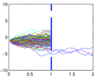
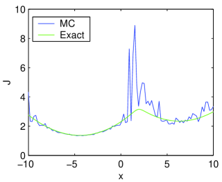
The left figure shows the trajectories of the sampling procedure for one particular value of $x$. Note, the inefficiency of the sampler because most of the trajectories are killed at the infinite potential at $t=t_{1}$. The right figure shows the accuracy of the estimate of $J(x,0)$ for all $x$ between $-10$ and $10$ using $N=100000$ trajectories. Note, that the number of trajectories that are required to obtain accurate results, strongly depends on the value of $x$ and $\lambda$ due to the factor $\exp(-\phi(x)/\lambda)$ in Eq. 12. For high $\lambda$ or low $\left<\phi\right>$, few samples are required (see the estimates around $x=-4$). For small noise or high $\left<\phi\right>$ the estimate is strongly determined by the trajectory with minimal $\phi(x(t_{f}))$ and many samples may be required to reach this $x$. In other words, sampling becomes more accurate for high noise, which is a well-known general feature of sampling. Also, low values of the cost-to-go are more easy to sample accurately than high values. This is in a sense fortunate, since the objective of the control is to move the particle to lower values of $J$ so that subsequent estimates become easier.

The sampling is of course particularly difficult in this example because of the infinite potential that annihilates most of the trajectories. However, similar effects should be observed in general due to the multi-modality of the Action.

We can improve the sampling procedure using the importance sampling procedure outlined in section 5.2, using the Laplace approximation. The Laplace approximation to $J$ requires the computation of the optimal deterministic trajectories. In general, one must use some numerical method to compute the Laplace approximation, for instance minimizing the Action Eq. 18 using a time-discretized version of the path. In this particular example, however, we can just write down the classical trajectories ’by hand’. For each $x$, there are two trajectories, each being piecewise linear. The Action for each trajectory is simply

$$S_{i}(x)=\frac{1}{2}R\int_{0}^{2}dt\dot{x_{i}}(t)^{2}=\frac{R}{2}(a_{i}-x)^{2}+\frac{R}{2}a_{i}^{2},\quad i=1,2$$

since $\phi(x(t_{f}))=V(x(t_{1}),t_{1})=0$ by construction. $a_{i}=6$ and $-4$ for the two trajectories, respectively. The cost-to-go in the Laplace approximation is given by Eq. 28:

$$J_{\mathrm{Laplace}}(x,0)=-\nu R\log\left(\exp\left(-\frac{S_{1}(x)}{\lambda}\right)+\exp\left(-\frac{S_{2}(x)}{\lambda}\right)\right)$$

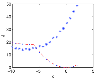
For each $x$, we randomly choose one of the two Laplace approximations with equal probability. We then sample according to Eq. 31 with $x^{*}$ the selected Laplace approximation and estimate $\psi$ using Eq. 29 and weights Eq. 32. The Laplace approximation and the results of the importance sampler are given in fig. 4.

Figure 4: Comparison of Laplace approximation (dotted line) and Monte Carlo importance sampling (solid jagged line) of $J(x,t=0)$ with exact result Eq. 33 (solid smooth line) for the double slit problem. The importance sampler used $N=100$ trajectories for each $x$. The parameters are as in fig. 2.

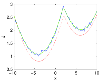
We see that the Laplace approximation is quite good for this example, in particular when one takes into account that a constant shift in $J$ does not affect the optimal control. The MC importance sampler dramatically improves over the naive MC results in fig. 3, in particular since 1000 times less samples are used and is also significantly better than the Laplace approximation.

6.1.2 The delayed choice

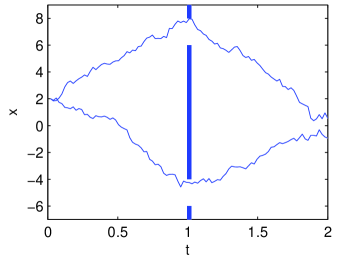
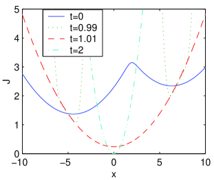
Finally, we show an example how optimal stochastic control exhibits spontaneous symmetry breaking. To simplify the mathematics, consider the double slit problem, when the size of the slits becomes infinitesimally small. Eq. 33, with $a=1,b=1+\epsilon,c=-1-\epsilon,d=-1$ becomes to lowest order in $\epsilon$:

$$J(x,t) = \frac{R}{T}\left(\frac{1}{2}x^{2}-\nu T\log 2\cosh\frac{x}{\nu T}\right)+\mathrm{const.}$$

where the constant diverges as ${\cal O}(\log\epsilon)$ independent of $x$ and $T=t_{1}-t$ the time to reach the slits. The expression between brackets is a typical free energy with inverse temperature $\beta=1/\nu T$. It displays a symmetry breaking at $\nu T=1$ (fig. 5a). For $T>1/\nu$ (far in the past) it is best to steer towards $x=0$ (between the targets) and delay the choice which slit to aim for until later. The reason why this is optimal is that from that position the expected diffusion alone of size $\nu T$ is likely to reach any of the slits without control (although it is not clear yet which slit). Only sufficiently late in time ($T<1/\nu$) should one make a choice. The optimal control is given by the gradient of $J$:

$$u=\frac{1}{T}\left(\tanh\frac{x}{\nu T}-x\right)$$ (34)

(a) Optimal cost-to-go at different $T$.

(b) Sample paths

Figure 5: (a) Symmetry breaking in $J$ as a function of $T$ implies a ’delayed choice’ mechanism for optimal stochastic control. When the target is far in the future, the optimal policy is to steer between the targets. Only when $T<1/\nu$ should one aim for one of the targets. $\nu=R=1$. (b) Sample trajectories (top row) and controls (bottom row) under stochastic control Eq. 34 (left column) and deterministic control Eq. 34 with $\nu=0$ (right column), using identical initial conditions $x(t=0)=0$ and noise realization.

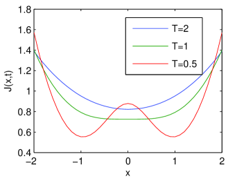
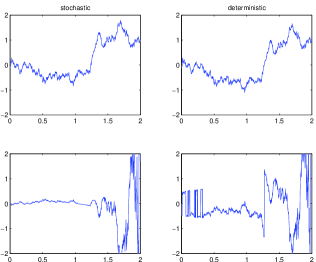
Figure 5b depicts two trajectories and their controls under stochastic and deterministic optimal control, using the same realization of the noise. Note, that at early times the deterministic control drives $x$ away from zero whereas in the stochastic control drives $x$ towards zero and smaller in size. The stochastic control maintains $x$ around zero and delays the choice for which slit to aim until $T\approx 1$.

The fact that symmetry breaking occurs in terms of the value of $\nu T$, is due to the fact that $S\propto 1/T$, which in turn is due to the fact that $u\propto 1/T$. Clearly, this will not be true in general. For an arbitrary control problem, $S$ does not need to be monotonic in $T$, which means that in principle control can be shifting back and forth several times between the symmetric and the broken mode as $T$ decreases to zero.

6.2 The drunken spider

In order to illustrate the drunken spider problem, we change the potential of the double slit problem so that it has a finite thickness: $V(x,t)=0$ for all $t<t_{1}$ and $t>t_{2}$ and for $t_{1}<t<t_{2}$:

$$V(x,t) = 0,\quad a<x<b,\quad c<x<d$$ (35)

$$= \infty,\quad\mathrm{else}$$

The problem is illustrated in Fig. 6 and the parameter values are given in the caption.

(a) Sample paths for $\nu=0.001$

(b) Sample paths for $\nu=0.1$

(c) $J(x,t=-1)$

Figure 6: The drunken spider problem. A spider located at $x$ and $t=-1$ wants to arrive home ($x=0$) at time $t_{f}$. The lake is indicated by the white square area, interrupted by a narrow bridge. The lake is modelled by the infinite potential given by Eq. 35 with $-a=b=0.1,c=-\infty$ and $d=-6$. $t_{1}=0,t_{2}=4,t_{f}=5$ and $R=1$. The cost-to-go is computed by forward importance sampling as outlined in section 5.2. The guiding Laplace approximations are the deterministic trajectories over the bridge and around the lake. Time discretization $dt=0.012$. (a) Some stochastic trajectories used to compute $J$ for $\nu=0.001$. (b) Some stochastic trajectories used to compute $J$ for $\nu=0.1$. (c) The optimal cost-to-go $J(x,t)$ in the Laplace approximation for $\nu=0.001$ and $\nu=0.1$ solid line (these two curves coincide). The MC importance sampling estimates are based on $1000$ trajectories per $x$ for $\nu=0.001$ (dots) and for $\nu=0.1$ (stars).

The cost-to-go in the Laplace approximation is given by Eq. 28, with $S(x(_{\alpha}(t\rightarrow t_{f})),\alpha=1,2$ the cost of getting home over the bridge or around the lake, respectively. It is plotted as a function of the current position $x$ as the solid line in fig. 6c, for both $\nu=0.001$ and $\nu=0.1$ (these two curves coincide for these values of $\nu$, since $S/\nu$ is so large that the softmax is basically a max).

In addition, we compute $J$ using importance sampling as outlined in section 5.2. For each $x$, we run $m=1000$ trajectories. For each trajectory, we select randomly one of the two Laplace trajectories with equal probability, which we denote by $x^{*}(t\rightarrow t_{f})$. The stochastic trajectory $x(t\rightarrow t_{f})$ is then computed from Eq. 31. It contributes to the partition sum Eq. 29 with a weight that is computed by Eq. 32, where $S_{\mathrm{path}}(x(t\rightarrow t_{f}))$ and $S^{\prime}_{\mathrm{path}}(x(t\rightarrow t_{f}))$ are given by Eq. 16 with $b(x(\tau),\tau)=0$ and $b(x(\tau),\tau)=x^{*}(\tau)$, respectively.

The results of the MC importance sampling for various $x$ for low noise ($\nu=0.001$) and high noise ($\nu=0.1$) are also shown in fig. 6c. The dots are the results of the MC importance sampling at low noise and closely follow the Laplace results. Note the discontinuous change in slope at $x=-6$, which implies a discontinuous change in the optimal control value $u$ at that point: For $x>-6$ the spider steers for the bridge, which requires a larger control value than for $x<-6$ when the optimal trajectory is around the lake. Thus, the optimal path is simply given by the shortest path and noise is ignored in these considerations.

The MC estimates for $\nu=0.1$ are indicated by the stars in fig. 6c. Since noise is large, the Laplace approximation is not valid, and indeed are very different from the MC estimate. The Laplace approximation ignores the effect of deviations from the deterministic trajectory on the Actions . Thus, it does not take into account that the spider may wander off the bridge and drowns, which at this level of noise will happen with almost probability one and makes $S_{\mathrm{bridge}}$ much larger than $S_{\mathrm{lake}}$. The MC importance sampling is guided by trajectories around the lake, that likely survive and by trajectories over the bridge, that will likely drown and thus will not contribute to Eq. 29. The estimate for $J$ is thus dominated by trajectories around the lake and the cost-to-go increases with increasing $x$. Also note, that the MC estimate puts the minimum of $J$ not at $x=-6$ but safely away from the lake, so that spider is not likely to fall in the lake on the low side either, and will have a safe journey home.

7 Discussion

In this paper, we have addressed the problem of computing stochastic optimal control. The direct solution of the HJB equation requires a discretization of space and time. This computation naturally becomes intractable in both memory requirement and cpu time in high dimensions. We have shown, that for a certain class of problems the control can be computed by a path integral. The class of problems includes arbitrary dynamical systems, but with a limited control mechanism. It includes LQ control as a special case. The path integral approach has the advantage that the $n$-dimensional $x$-space integration of the HJB equation is replaced by an $n$-dimensional sampling problem. For high-dimensional problems, a stochastic integration method is expected to be much more efficient than numerical integration of the HJB equation directly, which scales exponentially in $n$.

The obvious approximation methods to use are the Laplace approximation, the variational approximation and MC sampling. The Laplace approximation is very efficient. The deterministic trajectories are found by minimizing the action, which can be done by standard numerical methods. It typically requires ${\cal O}(n^{2}k^{2})$ operations, where $n$ is the dimension of the problem and $k$ is the number of time discretizations. We have seen that the multi-modal Laplace approximation gives non-trivial solutions involving symmetry breaking.

Computing the path integral by MC sampling is clearly a very generic approach, that for many practical control applications may well be the best way to go. Naive sampling should be replaced by more advanced sampling schemes. I have only considered one simple improvement using importance sampling. Other possible improvements could be a Gibbs sampler or a Metropolis-Hasting sampler. Clearly, more work in this direction must be done.

In this paper we have numerically computed the path integrals using the most simple discretization strategy: short time averaging [10]. The computation can be made much more efficient using Fourier discretization [11, 12] or other subspace approximations (compact splines or wavelets) [13]. In each of these methods the path integral is reduced to a high (but finite) dimensional Riemann integral, which is approximated using a Monte Carlo method. These more advanced discretizations can be combined with any of the mentioned MC methods.

I have not discussed the variational approximation in this paper. This approach to approximating the path integral is also known as variational perturbation theory and gives an expansion of the path integral in terms of the anharmonic interaction terms and a variational function that is to be optimized [14]. The lowest term in the expansion is similar to what is known as the variational approximation in machine learning using the Jensen’s bound [15], but one can also consider higher order terms. The expansion is around a tractable dynamics, such as for instance the harmonic oscillator, whose variational parameters are optimized such as to best approximate the path integral. The application of this method to optimal control would be the topic of another paper. A complication of such an analytic treatment is the presence of topological constraints, such as walls and obstacles.

There exist other fields of research that use path integrals and where dedicated numerical methods have been developed to solve them. For instance, in chemical physics path integrals are used to describe conformational changes in molecules over large time scales. The problem is similar to an optimal control problem such as navigating a maze: The begin and end positions are known, and one or more path of minimal cost needs to be found. A prominent method in this field is transition path sampling [16], which can be viewed as a Metropolis-Hasting sampling scheme in path space, where a new path is sampled by changing part of the current path and accepting the new path with a probability. This approach is probably also suitable for optimal control.

There is a superficial relation between the work presented in this paper and the body of work that seeks to find a particle interpretation of quantum mechanics. In fact, the $\log$ transformation was motivated from that work. Madelung [17] observed that if $\Psi=\sqrt{\rho}\exp(iJ/\hbar)$ is the wave function that satisfies the Schrödinger equation, $\rho$ and $J$ satisfy two coupled equations. One equation describes the dynamics of $\rho$ as a Fokker -Planck equation. The other equation is a Hamilton-Jacobi equation for $J$ with an additional term, called the quantum-mechanical potential which involves $\rho$. Nelson showed that these equations describe a stochastic dynamics in a force field given by the $\nabla J$, where the noise is proportional to $\hbar$ [8, 18].

Comparing this to the relation $\Psi=\exp(-J/\lambda)$ used in this paper, we see that $\lambda$ plays the role of $\hbar$ as in the QM case. However, the big difference is that there is only one real valued equation, and not two as in the quantum mechanical case. In the control case, $\rho$ is computed as an alternative to computing the HJB equation. In the QM case, the dynamics of $\rho$ and $J$ are computed together. The QM density evolution is non-linear in $\rho$ because the drift force that enters the Fokker-Planck equation depends on $\rho$ through $J$ as computed from the HJ equation.

References

- [1] L.S. Pontryagin, V.G. Boltyanskii, R.V. Gamkrelidze, and E.F. Mishchenko. The mathematical theory of optimal processes. Interscience, 1962.
- [2] R. Bellman and R. Kalaba. Selected papers on mathematical trends in control theory. Dover, 1964.
- [3] J Yong and X.Y. Zhou. Stochastic controls. Hamiltonian Systems and HJB Equations. Springer, 1999.
- [4] W.H. Fleming. Exit probabilties and optimal stochastic control. Applied Math. Optim., 4:329–346, 1978.
- [5] W.H. Fleming and H.M. Soner. Controlled Markove Processes and Viscosity solutions. Springer Verlag, 1992.
- [6] R. Stengel. Optimal control and estimation. Dover publications, New York, 1993.
- [7] L.F. Shampine, I. Gladwell, and S. Thompson. Solving ODEs with MATLAB. Cambridge University Press, 2003.
- [8] E. Nelson. Dynamical Theories of Brownian Motion. Princeton University Press, Princeton, 1967.
- [9] F. Guerra. Introduction to nelson stochastic mechanics as a model for quantum mechanics. In The Foundation of Quantum Mechanics, Amsterdam, 1995. Kluwer.
- [10] K.S. Schweizer, R.M. Stratt, D. Chandler, and P.G. Wolynes. Convenient and accurate discretized path integral methods for equilibrium quantum mechanical calculations. J.Chem. Phys., 75:1347–1364, 1981.
- [11] W.H. Miller. Path integral representation of the reaction rate constant in quantum mechanical transition state theory. J.Chem. Phys., 63:1166–1172, 1975.
- [12] D.L. Freeman and J.D. Doll. A monte carlo method for quantum boltzmann statistical mechanics using fourier representations of path integrals. J.Chem. Phys., 80:5709–5718, 1984.
- [13] S.D. Bond, B.B. Laird, and B.J. Leimkuhler. On the approximation of feynman-kac path integrals. Journal of Computational Physics, 185:472–483, 2003.
- [14] H. Kleinert. Path integrals in quantum mechanics, statistics,polymer physics and financial markets. MIT Press, 2004. Third edition.
- [15] R.P. Feynman and H. Kleinert. Effective classical partition functions. Physical Review A, 34:5080–5084, 1986.
- [16] P.G. Bolhuis, D. Chandler, Ch. Dellago, and P.L. Geissler. Transition path sampling: Throwing ropes over rough mountain passes, in the dark. Annu. Rev. Phys. Chem., 53:291–318, 2002.
- [17] E. Madelung. Z. Physik, 40:322, 1926.
- [18] F. Guerra. Structural aspects of stochastic mechanics and stochastic field theory. Physics Reports, 77:263–312, 1981.