LevelScheme: A level scheme drawing and scientific figure preparation
system for Mathematica

 

Abstract

LevelScheme is a scientific figure preparation system for Mathematica. The main emphasis is upon the construction of level schemes, or level energy diagrams, as used in nuclear, atomic, molecular, and hadronic physics. LevelScheme also provides a general infrastructure for the preparation of publication-quality figures, including support for multipanel and inset plotting, customizable tick mark generation, and various drawing and labeling tasks. Coupled with Mathematica’s plotting functions and powerful programming language, LevelScheme provides a flexible system for the creation of figures combining diagrams, mathematical plots, and data plots.

Program Summary

Title of program: LevelScheme

Catalogue identifier: ADVZ

Program summary URL: http://cpc.cs.qub.ac.uk/summaries/ADVZ

Program available from: CPC Program Library, Queen’s University of Belfast, N. Ireland

Operating systems: Any which supports Mathematica; tested under Microsoft Windows XP, Macintosh OS X, and Linux

Programming language used: Mathematica 4

Number of bytes in distributed program, including test code and documentation: 3 051 807

Distribution format: tar.gz

Nature of problem: Creation of level scheme diagrams. Creation of publication-quality multipart figures incorporating diagrams and plots.

Method of solution: A set of Mathematica packages has been developed, providing a library of level scheme drawing objects, tools for figure construction and labeling, and control code for producing the graphics.

PACS: 01.30.Rr

Keywords: level scheme; level energy diagram; drawing; plotting; figure preparation; Mathematica

 

I Introduction

LevelScheme is a scientific figure preparation system for Mathematica wolfram1999:mathematica-book-4 ; wolfram1999:mathematica-4 . The main focus is upon the construction of level schemes, or level energy diagrams, as used in several areas of physics, including nuclear, atomic, molecular, and hadronic physics. However, convenient preparation of publication-quality figures requires a variety of capabilities beyond those available with Mathematica’s built-in graphics display functions. The LevelScheme system thus also provides support for multipanel and inset plotting, customizable tick mark generation, and general drawing and labeling tasks. Coupled with Mathematica’s powerful programming language, plotting functions, and mathematical typesetting capabilities, LevelScheme is a flexible system for the creation of publication-quality figures. Figures can combine data plots, mathematical plots, and graphics generated by specialized packages (e.g., Ref. hahn2001:feynarts ) with diagrams constructed using LevelScheme’s drawing tools.

LevelScheme automates many of the tedious aspects of preparing a level scheme, such as positioning transition arrows between levels or placing text labels alongside the objects they label. The package allows extensive manual fine tuning of the drawing appearance, text formatting, and object positioning. It also includes specialized features for creating several common types of level schemes encountered in nuclear physics. Note that there already exist programs for drawing certain specific types of level schemes, such as band structure diagrams or decay schemes (e.g., Refs. radford1995:radware ; dunford2003:ensdat ).

After a discussion of the general features of the LevelScheme system (Sec. II), the major components of the software are considered in greater depth separately (Secs. III–V). Examples of the package’s graphical output are given in Sec. VI. The more technical details of using the LevelScheme package are addressed in the documentation provided through the CPC Program Library, which includes a tutorial discussion, a full reference guide, and extensive examples of code for producing figures with LevelScheme. Updates and further information may be obtained through the LevelScheme home page levelschemehome ; mathsourcecontribs .

II Principles of implementation

A few basic principles have guided the design of the LevelScheme system. One is that it should be possible for the user to make even major formatting changes to a level scheme relatively quickly. Objects are attached to each other (transition arrows are attached to levels, labels are attached to levels or transition arrows, etc.), so that if one object is moved the rest follow automatically. Another principle is for objects to have reasonable default properties, so that an unsophisticated level scheme can be drawn with minimal attention to formatting features. But the user must then be given extensive flexibility in fine tuning formatting details, to accomodate whatever special cases might arise. This is accomplished by making the more sophisticated formatting features accessible through various optional arguments (“options”) for which the user can specify values. The user can specify the values of options for individual objects, or the user can set new default values of options for the whole scheme to control the formatting of many objects at once. Finally, attention has been paid to providing a uniform user interface for all drawing objects, based upon a consistent notation for the specification of properties for the outline, fill, and text labels of objects.

The code for the LevelScheme system consists of essentially three parts. There is a library of functions made available to the user for drawing the individual objects within a figure (Sec. III). There are tools included to facilitate the general aspects of figure preparation and layout, such as construction of panels, axes, and tick marks (Sec. IV). And underlying these is a general infrastructure for managing the drawing process (option processing, coordinate system arithmetic, and a layered drawing system) and the final display of the figure (Sec. V).

III Drawing object library

The drawing object library is the portion of the LevelScheme system which is most visible to the user. Some of the objects in this library are specialized elements of level scheme diagrams, while others are general purpose drawing shapes and labels.

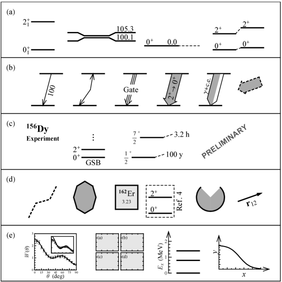
Figure 1: Drawing objects and figure components provided by the LevelScheme system. (a) Levels, extension lines, and connectors. (b) Transition arrows, including arrows with kinks, arrows with multiple shafts, extended shapes with outline and fill, and split-shading conversion electron transition arrows. (c) Labels, either stand-alone or attached in various ways to existing levels, making full use of Mathematica’s text-formatting capabilities. (d) Drawing shapes, including polylines, polygons, boxes, filled ellipses or arcs, and arrows. (e) Panels and axes, with extensive capability for labeling and tick customization.

The basic drawing objects are as follows:

1. An energy level object (Lev), consisting of a line and several attached labels. This line may have raised or lowered end segments (“gull wings”) to allow room for labels, as is customary in certain types of level schemes. There are also objects providing an extension line to the side of a level (ExtensionLine) or a connecting line between levels (Connector). These are shown in Fig. 1(a).

2. A transition arrow object (Trans), the endpoints of which can be automatically attached to two given levels or can be free-floating. This object is quite versatile. Labels can be attached to the transition arrow at predefined but adjustable positions, either aligned along the arrow or oriented as the user prefers. The arrow can be of several different styles ranging from a simple line to a filled polygonal arrow shape, with user control of all dimensions. Examples are shown in Fig. 1(b).

3. Separate label objects. Labels may be free-standing at coordinates specified by the user (ManualLabel and ScaledLabel) or may be positioned in relation to an existing level (BandLabel and LevelLabel). See Fig. 1(c).

4. General drawing objects. These are essentially enhanced versions of the basic Mathematica drawing primatives wolfram1999:mathematica-book-4 . They differ from the basic primatives in that their drawing properties are controlled through the LevelScheme option system and in that they conveniently combine an outline, fill, and text labels in a single object. The general drawing objects are an open curve or polyline (SchemeLine), a closed curve or polygon (SchemePolygon), a rectangle (SchemeBox), and a filled circular or elliptical arc (SchemeCircle). An arrow similar to Trans, but meant for general drawing and annotation tasks, is also provided (SchemeArrow). These are illustrated in Fig. 1(d).

The user creates a figure by providing a list of such objects to the drawing function Scheme (Sec. V). Each object’s position and appearance is governed by arguments. The most essential positioning information is indicated through a small number of mandatory arguments. The other aspects of the object’s positioning and appearance are specified as options, using the standard Mathematica option$\mathtt{\rightarrow}$value syntax wolfram1999:mathematica-book-4 , with extensions described in Sec. V.

Each drawing object is built from up to three distinct parts: an outline, a filled area, and attached text labels. The labels may contain any Mathematica expression and can take full advantage of Mathematica’s extensive typesetting capabilities. Several basic options controling the appearance of the object’s parts (e.g., Thickness, FillColor, and FontSize) are standardized across all object types, as are options for specifying the contents and positions of the text labels. Other options, such as those governing a level’s gull wings or an arrow’s shape, are specific to a given object type. If the user does not explicitly give a value for an option, its global default value is used. The user can thus control the style of all objects of a given type by changing the default setting of the relevant option, with SetOptions. For instance, the line thicknesses of the levels in a diagram can all be changed at once in this fashion, or the labels on these levels can be relocated from the top to the sides. The stylistic changes can be applied to the whole diagram or they can be made midway through, to affect only one portion of the diagram.

Let us consider a brief concrete example. The function used to draw a level object has syntax Lev[name,$x_{1}$,$x_{2}$,$E$], where the arguments are, respectively, a name chosen by the user, to be used to identify the level later so that other objects such as transition arrows can be attached to it, the left and right endpoint $x$ coordinates, and the energy or $y$ coordinate. The code needed to generate the leftmost diagram in Fig. 1(b) is then

    SetOptions[Lev, Thickness -> 2],
    Lev[lev0, 0, 1, 0],
    Lev[lev1, 0.3, 1.3, 10],
    Trans[lev1, lev0, LabR -> 100]

More extensive examples may be found in Appendix A and the documentation provided through the CPC Program Library.

IV Figure preparation tools

Mathematica provides a powerful system for generating graphics, but it does not by itself make available the fine formatting control necessary for the preparation of publication-quality figures. The relevant figure layout and tick customization tools provided by LevelScheme are summarized in this section.

Very often it is necessary to prepare figures with multiple parts. These range from simple side-by-side diagrams to more complicated possibilities, such as inset plots or rectangular arrays of plots with shared axes [Fig. 1(e)]. LevelScheme includes a comprehensive framework for assembling multipart figures.

The basic element of a multipart figure is a “panel”. This is a rectangular region designated as a plotting window within the full plot. Panels can be arranged within the figure as the user pleases, and they can arbitrarily overlap with each other. Each panel can have its own ranges defined for the $x$ and $y$ axes, as specified by the user. All objects are drawn with respect to these coordinates, as discussed further in Sec. V. If the user changes the position or size of the panel as a whole, all its contents thus move or are rescaled accordingly, without any need for changes to the arguments of the individual drawing objects.

A panel can be drawn with any of several ancillary components: a frame, tick marks, tick labels, axis labels on the edges of the frame, a panel letter, and a solid background color. All these characteristics are controlled by options to the basic panel definition command Panel. A panel can also simply be used without these, as an invisible structure to aid in laying out part of the figure. As an alternative to axis ticks on the panel frame, the object SchemeAxis allows stand-alone axes (including a line with optional arrow head, tick marks, tick labels, and an axis label) to be placed wherever needed within a figure [Fig. 1(e)].

The most common arrangement of figure panels is as a rectangular array [Fig. 1(e)]. The Multipanel tool greatly simplifies the construction of such an array. The user specifies a total region to be covered with the panels and the numbers of rows and columns of panels within this region, rather than calculating the position for each panel manually. The panels can be contiguous (shared edges) or separated by gaps, and different rows or columns of panels can have different heights or widths. The axes of the panels can be “linked”, as in many data plotting packages: The user specifies the $y$ axis range for each row and $x$ axis range for each column, and all panels within the row or column use this same range. The user can also specify the tick marks and axis labels by row and column. (Tick and axis labels are by default drawn only along the bottom and left exterior edges of the array as a whole.) Panels are automatically labeled with panel letters, formatted as chosen by the user. The user has the flexibility to override any or all of these automated settings on a panel by panel basis.

LevelScheme also supports detailed customization of tick mark placement and formatting. A very general function is provided to construct sets of tick marks. These tick marks can be used on panels, on stand-alone axes, and on the frame of the LevelScheme figure as a whole. (The built-in Mathematica plot display function can generate a default set of tick marks, but it does not give the user any control over the tick intervals or labels.) Linear, logarithmic, and general nonlinear axes are supported. For linear axes, the user specifies the start and end points of the coordinate range to be covered with tick marks and, optionally, the major tick interval and minor subdivisions. Options are used to control the appearance of the tick marks and formatting of the labels, or to suppress the display of certain tick marks or labels.

Beyond these basic tick mark formatting customizations, great flexibility is obtained through integration with the Mathematica functional programming language. Arbitrary nonlinear axes are obtained by specifying various transformation functions to be applied to the major and minor tick mark positions. Although the tick generation function provides basic fixed-point decimal label formatting, the user can instead specify an arbitrary function to generate the tick label from the tick coordinate. The resulting label can be any Mathematica text or symbolic expression and can involve complicated typesetting: for instance, plots of trigonometric functions might have tick labels written as rational multiples of the symbol $\pi$ (see examples in the documentation provided through the CPC Program Library). For convenience, a predefined function is provided for constructing logarithmic ticks with labels in the format $b^{n}$.

V Infrastructure

Let us now consider the technical framework underlying this LevelScheme figure construction process. This includes extensions to the Mathematica option passing scheme, definitions for handling a set of overlaid coordinate systems, a layered drawing system, and a mechanism for incorporating externally generated Mathematica graphics into the figure.

Options play a major role in LevelScheme’s approach to providing a simple but flexible drawing system and are used to control most aspects of the formatting of a level scheme. Two conceptual extensions to the standard Mathematica option passing scheme were needed to make this possible. Under the usual option system wolfram1999:mathematica-book-4 , default option values for a function are defined globally in the list Options[function], and these default values can be overriden by specifying an argument option$\mathtt{\rightarrow}$value when the function is invoked.

The user makes stylistic changes within a level scheme, affecting the appearance of all drawing objects of a given type, by setting the default values of relevant options, as discussed in Sec. II. However, if such a change were made to the usual global default value, it would have collateral effects on all other level schemes drawn in the same Mathematica session. To remedy this situation, LevelScheme implements dynamic scoping of default option value settings. The global default values are saved before processing of the scheme starts, and these original values are restored after processing finishes, so any changes made within a level scheme are confined to that scheme.

It is also sometimes convenient to have changes to certain basic stylistic options, such as the font size or line thickness, affect all objects in a drawing, not just those of a given type. To facilitate this, the concept of inheritance, from object oriented programming, has been applied to the Mathematica option system. All LevelScheme drawing objects are all defined to be child objects of a common parent object SchemeObject. The values of the basic outline, fill, and text style options (Sec. III) for these objects are by default taken, or inherited, from values set for SchemeObject. (Further details are given in Ref. mathsourcecontribs .)

Several different, complementary coordinate systems are needed to describe points within a LevelScheme figure (see Fig. 2). The Mathematica graphics display functions only recognize a single coordinate system, which runs from user-specified coordinates $(x_{1},y_{1})$ at the lower left corner of the figure to $(x_{2},y_{2})$ at the upper right corner. We refer to these coordinates as the “canvas coordinates”. All graphics coordinates must ultimately be expressed in terms of these for display by Mathematica.

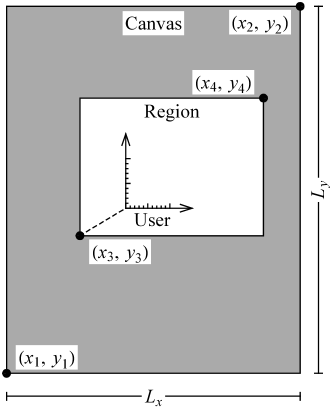
Figure 2: Overlaid coordinate systems maintained by LevelScheme: absolute (or physical), canvas, region, and user systems.

However, many drawing tasks require the calculation of physical distances as they will appear on the output page. Angles are not preserved under an unequal rescaling of the horizontal and vertical axes. Thus, for instance, construction of the right angled corners in arrows [Fig. 1(b)] requires knowledge of physical horizontal and vertical distances rather than just $x$ and $y$ coordinate distances. Since the physical dimensions $L_{x}$ and $L_{y}$ of the plotting region are known (Fig. 2), “absolute coordinates” measuring the physical position of a point within the figure can easily be related to the canvas coordinates.

For constructing multipart figures (Sec. IV), a smaller rectangular plotting region is designated within the full figure, with new ranges defined for the $x$ and $y$ axes within this region. The resulting “region coordinates” are fully determined if the coordinate values of the corners of the region, $(x_{3},y_{3})$ and $(x_{4},y_{4})$, are specified in both the canvas and region coordinate systems. These region coordinates are the basic coordinates defined within a plot panel. However, it is also convenient for the user to be able to arbitrarily shift portions of a diagram collectively, without individually modifying the coordinates specified for all the objects involved. This is accomplished by introducing “user coordinates”, which have a user-defined offset and scale relative to the region coordinates. (For instance, the individual diagrams were arranged from left to right within each panel of Fig. 1 by defining a different horizontal user coordinate offset before drawing the objects for each one.) The user specifies all coordinates for LevelScheme objects in the user coordinate system. Initially, the canvas, region, and user coordinate systems for a figure are identical. Each time the user redefines the coordinates, e.g., by defining a panel or introducing a user coordinate offset, the affine transformation coefficients relating the various coordinate systems are recalculated and stored.

A final important component of the drawing infrastructure is the layered drawing system. Each drawing element is assigned to a numbered layer. Those assigned to lower-numbered layers (background) are rendered before, and thus might be hidden by, objects assigned to higher-numbered layers (foreground). The layering system is essential for preventing text labels from being hidden by other drawing elements in dense level schemes. By default, outlines and fills are assigned to layer 1, “white-out” boxes behind text labels are in layer 2, and the text itself is in layer 3. With this layering system, white-out boxes hide any lines or fills behind them, but they do not block neighboring text, making possible closely-spaced transition labels, such as are needed in decay schemes (see Sec. VI for examples).

Arbitrary Mathematica graphics, including the output of the Mathematica plotting routines, can be incorporated into a LevelScheme figure. Mathematica represents graphical output as a Graphics object containing a list of “primatives” wolfram1999:mathematica-book-4 , which are either drawing elements (polylines, polygons, points, etc.) or directives affecting the style in which the following drawing elements are rendered (color, thickness, dashing). For inclusion in a LevelScheme figure, such graphics must be “wrapped” in a LevelScheme RawGraphics object, which extracts the primatives from the Graphics object and carries out several manipulations on them. It first transforms all the coordinates contained in the graphics primatives from user coordinates to canvas coordinates, thereby moving and scaling the graphics to appear according to the user’s current choice of coordinate system. (The graphics may contain coordinates given in the special Offset and Scaled notations defined by Mathematica.) It then clips all polylines and polygons to the current plot region, using a standard algorithm sutherland1974:polygon-clipping . Finally, it supplies default drawing style primatives and a layer number for the graphics, for use by the layered drawing system.

The graphical content of a LevelScheme figure is assembled by the function Scheme. The user provides a list of LevelScheme drawing objects to Scheme. Intermixed with these objects may be commands, such as SetOptions or Panel, which affect the appearance of the following objects. Scheme also accepts options governing the overall figure properties (plot range, dimensions, frame labels and ticks, etc.) much like the usual Mathematica plotting functions. The final output of Scheme is a Graphics object.

We can now summarize the steps carried out by Scheme in creating a figure. The list of objects passed to scheme is initially “held” in unevaluated form, contrary to the usual Mathematica symbolic evaluation rules, to prevent premature evaluation of the coordinate arithmetic expressions and any SetOptions calls it contains. Scheme first initializes the variables controlling the overlayed coordinate systems, based upon the plot range and image dimensions specified by the user. Scheme then evaluates the list of objects, dynamically scoping the drawing object default option values as described above. Evaluation of the objects relies upon three standardized functions for generating outlines, fills, and text labels. These functions in turn each return a structure containing three parts: a list of graphics style primatives based upon the LevelScheme style option values (Sec. III), a list of primatives for the drawing elements, and a layer number. Scheme sorts the resulting structures in order of ascending layer number, to insure that drawing elements in foreground layers are rendered after those in background layers, and then discards the layer information, extracting just the graphics primatives. Since many consecutive objects typically have the same drawing style properties, Scheme achieves considerably more compact output by stripping redundant style primatives from the list. Scheme also constructs frame and axis directives for the whole scheme, which are combined with the graphics primative list to make a Mathematica Graphics object.

VI Graphical output examples

Several examples of figures generated using the LevelScheme system are shown in this section. These figures, mainly level scheme diagrams, have been chosen to demonstrate several of the capabilities discussed in the earlier sections and to illustrate the variety of drawing styles possible.

Figs. LABEL:fig154dycascades and LABEL:fig102pd0plus are basic level schemes, as might be encountered in presentations. Note the various arrow styles and arrow label positions. The complete code used to generate Fig. LABEL:fig154dycascades is given in Appendix A.

Fig. LABEL:fig166hfbeta is in the classic style for a decay scheme, showing $\gamma$-ray transitions among nuclear levels populated following $\alpha$ or $\beta$ decay. LevelScheme provides tools which automate the positioning of the equally-spaced vertical transition arrows in such decay schemes. Note the gull wings on the levels and the white-out boxes behind the transition labels. The layered drawing system discussed in Sec. V prevents these boxes from obstructing neighboring labels.

Fig. LABEL:figtriaxschemes is an example of a multipanel figure involving only level schemes. Fig. LABEL:figcombo combines a level scheme diagram with function and data plots.

Fig. LABEL:fige5reference is a larger-scale scheme, involving bent arrows. Heavy use is made of annotation labels beside or below levels. In such a scheme, user coordinate offsets simplify adjustment of the horizontal spacing between the different families of levels.

Fig. LABEL:fignchart provides an illustration of the use of LevelScheme drawing tools for technical diagrams other than level schemes. Mathematica’s programming language can be used to automate the construction of complex diagrams containing large numbers of drawing objects. Nuclear charts are simple to create using the SchemeBox drawing object, which provides the outline, fill, and labels for each cell. The entire array of cells can be constructed by using a single Mathematica Table construct to iterate over proton and neutron numbers. (Mathematica’s chemical elements database provides the element symbols and information on which nuclides are stable.) The resulting chart can be overlaid with a Mathematica contour plot, as in Fig. LABEL:fignchart (left), where the LevelScheme layered drawing system has been used to ensure that labels appear in front of the contour lines. Information read from external data files can be superposed as well, in the form of cell colors, cell text contents, or region boundary lines, as in Fig. LABEL:fignchart (right).

VII Conclusion

The LevelScheme system for Mathematica provides a flexible system for the construction of level energy diagrams, automating many tedious aspects of the preparation while allowing for extensive manual fine-tuning and customization. The general figure preparation tools and infrastructure developed for this purpose also have broad applicability to the preparation of publication-quality multipart figures with Mathematica, incorporating diagrams, mathematical plots, and data plots.

Appendix A Figure source code

This appendix contains the Mathematica code used to generate Fig. LABEL:fig154dycascades with the LevelScheme figure preparation system.

    Scheme[{

      (* set default styles for level scheme objects *)

      SetOptions[SchemeObject, FontSize -> 20];
      SetOptions[Lev, NudgeL -> 1, NudgeR -> 1, LabR -> Automatic],
      SetOptions[Trans, ArrowType -> ShapeArrow, HeadLength -> 9, HeadLip -> 10, Width -> 30,
        FontColor -> Blue, OrientationC -> Horizontal, BackgroundC -> Automatic],
      SetOptions[LevelLabel, Gap -> 10],

      (* draw cascade from 4+ level *)

      SetOrigin[0],
      ManualLabel[{-.4, 850}, "(a)", Offset -> {-1, 1}],

      Lev[lev0, 0, 2, "0", LabL -> LabelJP[0]],
      Lev[lev335, 0, 2, "335", LabL -> LabelJP[2]],
      LevelLabel[lev335, Right, "27 ps"],
      Lev[lev661, 0, 2, "661", LabL -> LabelJP[0]],
      Lev[lev747, 0, 2, "747", LabL -> LabelJP[4]],
      LevelLabel[lev747, Right, "  6 ps", FontColor -> Red],
      Trans[lev335, 1.3, lev0, Automatic, FillColor -> LightGray, LabC -> "TIMING"],
      Trans[lev747, .7, lev335, Automatic, FillColor -> White, LabC -> "GATE"],

      (* draw cascade from 0+ level *)

      SetOrigin[3.5],
      ManualLabel[{-.4, 850}, "(b)", Offset -> {-1, 1}],

      Lev[lev0, 0, 2, "0", LabL -> LabelJP[0]],
      Lev[lev335, 0, 2, "335", LabL -> LabelJP[2]],
      LevelLabel[lev335, Right, "27 ps"],
      Lev[lev661, 0, 2, "661", LabL -> LabelJP[0]],
      LevelLabel[lev661, Right,
        RowBox[{"$\mathtt{\tau}$(", hspace[-0.2], LabelJiP[0, 2], ")"}],
        FontColor -> Red],
      Lev[lev747, 0, 2, "747", LabL -> LabelJP[4]],
      Trans[lev335, 1.3, lev0, Automatic, FillColor -> LightGray, LabC -> "TIMING"],
      Trans[lev661, .9, lev335, Automatic, FillColor -> White, LabC -> "GATE"],

      },
    PlotRange -> {{-.8, 6.3}, {-100, 900}}, ImageSize -> 72*{8, 4}
    ];

References

- (1) S. Wolfram, The Mathematica Book, 4th ed. (Wolfram Media/Cambridge University Press, 1999).
- (2) Wolfram Research, Inc., Mathematica 4 (Champaign, Illinois, 1999).
- (3) T. Hahn, Comput. Phys. Commun. 111 (1998) 217.
- (4) D. C. Radford, Nucl. Instrum. Methods A 361 (1995) 297.
- (5) C. L. Dunford and R. R. Kinsey, computer code ENSDAT (unpublished).
- (6) Updates and further information may be obtained through the LevelScheme home page (http://wnsl.physics.yale.edu/levelscheme).
- (7) The BlockOptions, CustomTicks, ForEach, and InheritOptions components of the LevelScheme system have previously been made available through the Mathematica Information Center’s MathSource code library (http://library.wolfram.com/infocenter), where further technical documentation may be found.
- (8) I. E. Sutherland and G. W. Hodgman, Commun. ACM 17 (1974) 132.
- (9) M. A. Caprio, Ph.D. thesis, Yale University (2003), eprint arXiv:nucl-ex/0502004.
- (10) E. A. McCutchan, N. V. Zamfir, R. F. Casten, M. A. Caprio, H. Ai, H. Amro, C. W. Beausang, A. A. Hecht, D. A. Meyer, and J. J. Ressler, Phys. Rev. C 71 (2005) 024309.
- (11) M. A. Caprio and F. Iachello, Ann. Phys. (N.Y.) 318 (2005) 454.
- (12) M. A. Caprio, J. Phys. A 38 (2005) 6385.
- (13) M. A. Caprio, in Nuclei and Mesoscopic Physics, edited by V. Zelevinsky, AIP Conf. Proc. No. 777 (AIP, Melville, New York, 2005), p. 199.