The Community Structure of Econophysicist Collaboration Networks

Abstract

This paper uses a database of collaboration recording between Econophysics Scientists to study the community structure of this collaboration network, which with a single type of vertex and a type of undirected, weighted edge. Hierarchical clustering and the algorithm of Girvan and Newman are presented to analyze the data. And it emphasizes the influence of the weight to results of communities by comparing the different results obtained in different weights. A function D is proposed to distinguish the difference between above results. At last the paper also gives explanation to the results and discussion about community structure.

Keyword: Weighted Networks, Community Structure, Dissimilarity

PACS: 89.75.Hc 05.40.-a 87.23.Kg

1 Introduction

In recent years, as more and more systems in many different fields can be depicted as complex networks, the study of complex networks has been gradually becoming an important issue. Examples include the world wide web, social networks, biological networks, food webs, biochemical networks and so on[1, 19, 2, 9, 6, 20]. As one of the important properties of networks, community structure attracts us much attention. Community structure is the groups of network vertices. Within the groups there have dense internal links among the nodes, but between groups the nodes loosely connected to the rest of the network[8]. Communities are very useful and critical for us to understand the functional properties of complex structure better. So the problem of detecting and analyzing underlying communities is an important mission to us.

The idea of finding communities is closely related to the graph partitioning in graph theory, computer science and sociology[5]. The study of community structure in networks has a long history, so several types of algorithms have been developed for finding the community structure in networks. Early algorithms such as Spectral bisection[4] and the Kernighan-Lin algorithm[4] perform poorly in many general cases. To overcome the problems, in recent years, many new algorithms have been proposed[8, 10, 11, 12, 13]. As one of these algorithms, the algorithm of Girvan and Newman (GN) is the most successful one. It is a divisive algorithm. The idea behind it is edge betweenness, a generalization of the betweenness firstly introduced by Freeman[14]. The betweenness of an edge in network is defined to be the number of the shortest paths passing through it. It is very clearly that edges which connect communities, as all shortest paths connect nodes in different communities have to run along it, have a larger betweenness value. By removing the edge with the largest betweenness at each step, we can gradually split the whole network into isolated components or communities.

The application of GN algorithm has acquired successful results to different kinds of networks[8, 9]. Such as in [9], the authors use the GN algorithm to study the community structure of the collaboration network of jazz musicians. The analysis to the results reveals the presence of communities which have a strong correlation with the recording location of the bands, and also shows the presence of racial segregation between the musicians.

In recent years, most of the real-worlds which have been studied were represented as non-weighted networks by neglecting lots of data. The researchers paid more attention to the communities under the influence of the topology of the network. However, the weight of edges is important and may affect the results of communities, and it can tell us more information than whether the edge is present or not. For example, in a social network there are stronger or poorer connections between individuals, and the weight of edges are applied to describe the different strengths. So when we try to detect communities in this network, we should consider the weights into the process. It may give us better results closely according with facts than ignoring them.

In [21], we built an Econophysics Scientific Collaboration Network and gave some statistical results about this network. In this paper, we focus on the investigation of community structure of this network. We get the results of communities by using GN algorithm and hierarchical clustering. We also obtained the communities in different conditions including weighted, non-weighted, and different weights. In latest months, Newman has pointed out that applying the original GN algorithm to the weighted networks would obtain poor results, and gave the generalization of the GN algorithm to a weighted network[22]. In [5], Newman and Girvan define a function Q to measure where the best division for a given network, and also a generalization of Q to the weighted networks was proposed in this paper. We applied it to our network and found the peaks of Q correspond closely to the expected divisions.

The outline of this article is as follows. In Section 2 we describe in detail our work. First, we introduce our database and the Econophysics Scientific Collaboration Network which was built on the database briefly. Then we describe the algorithms and the definition of the different weights that were used to find underlying communities in our network. At last, we give the results by each condition and the compare between them. In Section 4 we give our conclusions.

2 The communities acquired by different algorithms

A network is composed of a set of vertices and edges which represent the relationship between the two nodes. In the Econophysicist collaboration network[21], each node represents one scientist. If the two scientists have collaborated one or more papers, they would be connected by an edge. In order to distinguish the different level of collaboration, we define the weights on the edges. So it’s a weighted network. Here we take the largest cluster from the network as the subject of our research. It is a sparse network including 271 nodes and 371 edges.

The weight is the crucial factor in our network analysis. Edge weights represent the strength or capacity of the edges. The weight of this network is defined as: $w_{ij}=tanh(t_{ij})$, where $t_{ij}$ is the number of papers which the researchers have collaborated. The reason we prefer the $\tanh$ function in empirical studies is that, first, it has the saturation effect, which makes the contribution less for larger connecting times; second, it normalizes the maximum value to $1$, which is the usual strength of edge in non-weight networks[21]. As the similarity is used here as the weight, the larger the weight is, the closer the relation between the two ends nodes is. The weight and connection provide us a natural description for the distance of two nodes.

In this part, we present two methods, hierarchical clustering and the algorithm of GN, on the analysis of community structure in our network. Because GN algorithm performs well in many networks and hierarchical clustering is the principal technique used in social networks in current.

In practical situation the algorithms will normally be used on networks for which the communities are not known ahead of time. This raises a new problem: how do we know when the communities found by the algorithm are good ones? To answer this question, in [3], Newman proposed a measure of the quality of a particular division of a network, which they call it the modularity. Then they define a modularity measure by

$$Q=\frac{1}{2m}\sum_{ij}[A_{ij}-\frac{k_{i}k_{j}}{2m}]\delta(c_{i},c_{j})$$ (1)

This quantity measures the fraction of the edges in the network that connect nodes of the same community minus the expected value of the same quantity in a network with the same community division but random connections between the vertices. $A_{ij}$ represents the edge between nodes $i$ and $j$, the degree $k_{i}$ is defined as $k_{i}=\sum_{j}A_{ij}$ , and $m=\frac{1}{2}\sum_{ij}A_{ij}$. $c_{i}$ is the community to which vertex $i$ is assigned. Newman has generalized the above measure to weighted networks[22]. Here we use the similar formula to our weighted network with similarity weight range from 0 to 1:

$$Q=\frac{1}{2m}\sum_{ij}[w_{ij}-\frac{w_{i}w_{j}}{2m}]\delta(c_{i},c_{j})$$ (2)

where $w_{ij}$ represents the weight in the edge between nodes $i$ and $j$, $w_{i}$ is the weight of node $i$: $w_{i}=\sum_{j}w_{ij}$ , and $m=\frac{1}{2}\sum_{ij}w_{ij}$.

Using hierarchical clustering method to find communities, we start from an empty graph with all nodes and no edges. Then we connect the edges in order of decreasing similarity. In our network, we use the measure $d_{ij}$ which describes the similarity to be the short path between a pair $(i,j)$ of vertices, where the shorter path represents the bigger similarity. When the nodes are clustered to be the communities, we define the distance between different communities as follows

$$D_{pq}=\max_{i\in p,j\in q}d_{ij}.$$ (3)

$p,q$ are any two communities. The measure $d_{ij}$ equals to the shortest path between a pair $(i,j)$ of vertices.

We have got the result from above hierarchical clustering method. It shows the modules in this result and also a peak in $Q$ function. The best division has 23 clusters.

GN method has got better results for community analysis. As mentioned in the section of introduction, the idea behind the algorithm of GN is edge betweenness. And the betweenness of an edge is defined to be the number of the shortest paths passing through it. To search the shortest paths between any two vertices, we use the Dijkstra algorithm. For the determination of shortest path, the similarity weight $w_{ij}\in\left[0,1\right]$ has been transformed to dissimilarity weight by $\tilde{w}_{ij}=\frac{1}{w_{ij}}$, and then $\tilde{w}_{ij}\in\left[1,\infty\right]$ is corresponding to the ”distance” between nodes. All paths are calculated under this dissimilarity weight from now on if not mentioned. The principal ways of GN algorithm are as follows [5]:

1.Calculate betweenness scores for all edges in the network.

2.Find the edge with the highest score and remove it from the network.

3.Recalculate betweenness for all remaining edges.

4.Repeat from step 2 until all links are removed.

The best result given by maximum $Q$ has 10 clusters. The GN algorithm and the hierarchical clustering which are based on the equation 3 all show the modules in the results. In the best divisions, we analyze the communities with the data. The results of algorithm of GN is better than hierarchical clustering. Because the result in the best division of GN algorithm shows that the scientists, who are in the same university, institute or interested in similar research topic, are clustered to one community. It is close to the reality. For example, in figure 1 the members of the red community are most from Boston University USA. And there are other communities which the members are focused on the same topic, as the yellow one. Meanwhile even the hierarchical clustering shows the modules, the result is not consistent with the reality.

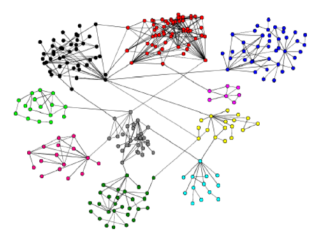
Figure 1: The best division of Econophysics Scientist Collaboration Network, with the divisions detected by GN algorithm represented by different colors.

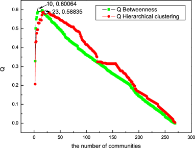
Figure 2: The comparison of modularity detected by GN algorithm and hierarchical clustering with Maximum minimum method. The peak are in 10 and 23 clusters respectively.

3 The comparison of different formation of communities

In the above section, we obtained that the results of GN algorithm and hierarchical clustering are different. How to quantify the difference between them? We define a function $D$ to measure it. The idea behind the function is to discuss the similarity and dissimilarity between sets $A$ and $B$. Let’s discuss the similarity and dissimilarity of two sets $A$ and $B$ defined as subset of $\Omega$. The idea is quite trivial, the similarity is represented by $A\cap B$, the dissimilarity should corresponds to $\left(A\cap\bar{B}\right)\cup\left(\bar{A}\cap B\right)$. Therefore, the normalized similarity and dissimilarity can be defined as

$$\left\{\begin{array}[]{l}s=\frac{\left|A\cap B\right|}{\left|A\cup B\right|}\\ \\ d=\frac{\left|\left(A\cap\bar{B}\right)\cup\left(\bar{A}\cap B\right)\right|}{\left|A\cup B\right|}\end{array}\right..$$ (4)

In a way more convenient to be generalized to classification systems with more than only two sets, we can rewrite above expression by the characteristic mapping of set $sign\left(X,\omega\right)$, which is defined as following,

$$sign\left(X,\omega\right)=\left\{\begin{array}[]{ll}1&\mbox{for }\omega\in X\\ \\ 0&\mbox{for }\omega\bar{\in}X\par\end{array}\right..$$ (5)

This mapping from $X$ to $\left\{1,0\right\}$ can be very machinery calculated for any element $\omega$ in $\Omega$ and for any subset $X$. It’s easy to check

$$\left\{\begin{array}[]{l}\left|A\cap B\right|=\sum_{\omega\in\Omega}sign\left(A,\omega\right)sign\left(B,\omega\right)\\ \\ \left|\left(A\cap\bar{B}\right)\cup\left(\bar{A}\cap B\right)\right|=\sum_{\omega\in\Omega}\left|sign\left(A,\omega\right)-sign\left(B,\omega\right)\right|\end{array}\right..$$ (6)

And also

$$\left|A\cup B\right|=\left|A\cap B\right|+\left|\left(A\cap\bar{B}\right)\cup\left(\bar{A}\cap B\right)\right|$$ (7)

Therefore, by the characteristic mapping, the similarity and dissimilarity are reexpressed by

$$\left\{\begin{array}[]{l}s=\frac{\sum_{\omega\in\Omega}sign\left(A,\omega\right)sign\left(B,\omega\right)}{\sum_{\omega\in\Omega}\left[sign\left(A,\omega\right)sign\left(B,\omega\right)+\left|sign\left(A,\omega\right)-sign\left(B,\omega\right)\right|\right]}\\ \\ d=\frac{\sum_{\omega\in\Omega}\left|sign\left(A,x\right)-sign\left(B,\omega\right)\right|}{\sum_{\omega\in\Omega}\left[sign\left(A,\omega\right)sign\left(B,\omega\right)+\left|sign\left(A,\omega\right)-sign\left(B,\omega\right)\right|\right]}\end{array}\right..$$ (8)

Consider a particular division of a network into $k$ communities. There are two formations of $k$ communities by different algorithms. we can deduce the comparison of them into many pairs of comparison between sets.The principal way is:

1. Construct the correspondence between the two subsets from different conditions

2. Compare every corresponding pair.

3. At last, integrate all the results from comparison of every single pair.

Correspondence relation here means, for every subset $X_{i}$ in classification $X_{k}$, to find the counterpart $Y_{i}$ in $Y_{k}$, by the similarity measurement. Here $X_{i}$ and $Y_{i}$ correspond to above $A$ and $B$. After that we will get two ordered set $X$ and $Y$, where the elements at the corresponding order are a pair of counterparts. And then apply the dissimilarity measure onto every pair to get a measurement of the total dissimilarity.

$$D=\frac{\sum_{i=1}^{k}{d_{X_{i}Y_{i}}}}{k}$$ (9)

Under this definition, $d$ will be normalized in $\left[0,1\right]$, where $\left(0,1\right)$ means no and large difference respectively.

The principle of the first step is to compare every single set $X_{i}$ from $X$ with all the $Y_{i}$ in $Y$, and group it with the one having largest similarity. However, at some cases, this may lead to a very ugly correspondence, for instance, many $X_{i}$ correspond to the same $Y_{i}$. at this time, we choose the largest one of them and group the $X_{i}$ which correspond the largest one with the $Y_{i}$. other $X_{i}$ should found the counterpart again in rest $Y_{i}$. But in some times, we want to discuss the different formations of communities, for example, we want to compare the dissimilar between the best division of GN algorithm and hierarchical clustering. As obtained above, we know that the number of communities are different. it meant some $Y_{j}$ in hierarchical clustering don’t have any counterparts. In this case, the first step still can be done by treating the whole group as a large subset, and treating no counterpart as empty set $\Phi$. The $k$ equal to the larger number. Here we give two examples, the first one, a network, including $N$ nodes, was divided into two communities by two algorithms. One division is two equal communities. The other division is a node and the rest nodes. Calculating the dissimilar of two algorithm, we got $d\approx 0.75$. The second example is a network, including $N$ nodes, was divided into $N$ communities. calculating the dissimilar of the whole network and the $N$ communities, $d\approx 1$.

We use this algorithm to analyze the dissimilar of hierarchical clustering and GN algorithm, and the result was shown in figure 3. With the same number of communities, the $Q$ curves and dissimilarity $D$ for the results from different algorithm are shown. we also focus on the dissimilar of best division of them, $D_{best}=0.756$, which means they are quite different.

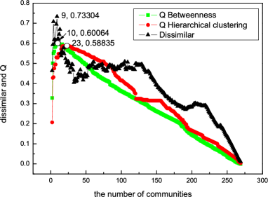
Figure 3: The dissimilarity $D$ of the results from hierarchical clustering and GN algorithm with same clusters.

3.1 The influence of weight to the results of communities

Now we turn to the effects of weight on the community structure of weighted networks. In [23], in order to study the impaction of weight to the topological properties of network,we have introduced the way to re-assign weights onto edge with $p=1,-1$ for weighted networks. Set $p=1$ represents the original weighted network given by the ordered series of weights which gives the relation between weight and edge but in a decreasing order,

$$W(p=1)=\left(w_{i_{1}j_{1}}=w^{1}\geq w_{i_{2}j_{2}}=w^{2}\geq\cdots\geq w_{\left(i_{L}\right)\left(j_{L}\right)}=w^{L}\right).$$ (10)

$p=-1$ is defined as the inverse order as

$$W(p=-1)=\left(w_{i_{1}j_{1}}=w^{L}\leq\cdots\leq w_{\left(i_{L-1}\right)\left(j_{L-1}\right)}=w^{2}\leq w_{\left(i_{L}\right)\left(j_{L}\right)}=w^{1}\right),$$ (11)

In this paper, we use the comparison of the communities which formed in non-weighted and re-assign weights onto edges with $p=1,-1$ to show the influence of weight to the results of communities.

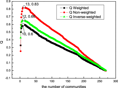
Figure 4: the Q of different weights in GN algorithm

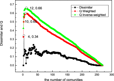
Figure 5: A: The dissimilarity of non-weighted and weighted network in GN algorithm. The dissimilarity of the best division is: $D_{10,13}=0.42$. B: The dissimilarity of weighted and inverse weighted network in GN algorithm. The dissimilarity of the best division is: $D_{10,12}=0.25$.

We obtained the influence of weight to the results of communities from the function Q and the dissimilarity. Using GN algorithm to detect communities, the influence of weight were shown in figure 4,5. In the figure 4, although the communities number of best division in different weights are quite same, the components of each community are quite different. The same things happened in using hierarchical clustering to analyze the network. Comparing these figures, we found that the weight have bigger influence in GN algorithm.

4 Concluding Remarks

In this paper, we study the community structure of scientists collaboration network by using hierarchical clustering algorithm and the algorithm of GN. And we also pay much attention to the influence of the weight to results of communities. It has been found that GN algorithm gives better results. Scientists who are in the same university, institute or interested in similar research topic are clustered to one community. In order to study the topological role of the weight, we have introduced a measure to describe the difference of two kinds of communities. Then we investigate the different results of clustering for non-weighted, weighted, and inverse weighted networks. The weight do have influence on the formation of communities but it is not very significant for our network of econophysicits. We guess that maybe our network is a sparse network, so the existence or not of edges have bigger influence to community structure of networks than the weight.

References

- [1] R. Albert and A.-L. Barabási, Rev. Mod. Phys. 74, 47 (2002).
- [2] M. E. J. Newman, The structure and function of complex networks, SIAM Review 45, 167-256 (2003).
- [3] M. E. J. Newman, M. Girvan, Mixing patterns and community structure in networks,in Statistical Mechanics of Complex Networks, R. Pastor-Satorras, J. Rubi and A. Diaz-Guilera (eds.), pp. 66-87, Springer, Berlin (2003)
- [4] M. E. J. Newman, Detecting community structure in networks, Eur. Phys. J. B 38, 321-330 (2004).
- [5] M. E. J. Newman and M. Girvan, Finding and evaluating community structure in networks, Phys.Rev. E 69, 026113 (2004).
- [6] M. E. J. Newman, Coauthorship networks and patterns of scientific collaboration, Proc. Natl. Acad. Sci. USA 101, 5200-5205 (2004).
- [7] F. Radicchi, C. Castellano, F. Cecconi, V. Loreto, and D. Parisi, Defining and identifying communities in networks, Proc. Natl. Acad. Sci. USA 101, 2658-2663(2004).
- [8] M. Girvan and M. E. J. Newman, Community structure in social and biological networks, Proc. Natl. Acad. Sci. USA 99, 7821-7826 (2002).
- [9] Community structure in jazz.
- [10] Fang Wu, B.A. Huberman, Finding Communities in Linear Time: A Physics Approach, cond-mat/0310600.
- [11] J. Reichardt, S. Bornholdt, Detecting fuzzy community structures in complex networks with a Potts model, cond-mat/0402349.
- [12] S. Fortunato, V. Latora, M. Marchiori, A Method to Find Community Structures Based on Information Centrality, cond-mat/0402522.
- [13] Luca Donetti and Miguel A. Muñoz, Detecting Network Communities: a new systematic and efficient algorithm, cond-mat/0404652
- [14] L. Freeman, A set of measure of centrality based upon betweenness, Sociometry 40, 35 (1977).
- [15] M. E. J. Newman, The structure of scientific collaboration networks, Proc. Natl. Acad. Sci. USA 98, 404-409 (2001).
- [16] C.-M. Ghima, E. Oh, K.-I. Goh, B. Kahng, and D. Kim, Packet transport along the shortest pathways in scale-free networks, Eur. Phys. J. B 38, 193-199 (2004).
- [17] R.Guimerà, L. Danon, A. Díaz-Guilera, F. Giralt, and A. Arenas, Self-similar community structure in a network of human interactions, Phys. Rev. E 68, 065103 (2003).
- [18] Haijun Zhou, Distance, dissimilarity index, and network community structure, Phys. Rev. E67, 061901 (2003)
- [19] R. Albert, H. Jeong, and A.-L. Barabaái, Nature 401, 130-131(1999).
- [20] R. J. Williams and N. D. Martinez, Simple rules yield complex food webs, Nature 404, 180-183 (2000).
- [21] Ying Fan Menghui Li, Jiawei Chen, Liang Gao, Zengru Di, Jinshan Wu. Network of Econophysicists: A Weighted Network to Investigate the Development of Econophysics. International Journal of Modern Physics B, vol18, (17-19), 2505-2511(2004).
- [22] M. E. J. Newman, Analysis of weighted networks, Phys. Rev. E. 70. 056131(2004).
- [23] Menghui Li, Zengru Di, Jiawei Chen, Liang Gao and Jinshan Wu, Weighted networks of scientific communication: the measurement and topological role of weight, Physica A 350 643-656(2005).